Consistency of community detection in networks under degree-corrected stochastic block models

Abstract

Community detection is a fundamental problem in network analysis, with applications in many diverse areas. The stochastic block model is a common tool for model-based community detection, and asymptotic tools for checking consistency of community detection under the block model have been recently developed. However, the block model is limited by its assumption that all nodes within a community are stochastically equivalent, and provides a poor fit to networks with hubs or highly varying node degrees within communities, which are common in practice. The degree-corrected stochastic block model was proposed to address this shortcoming and allows variation in node degrees within a community while preserving the overall block community structure. In this paper we establish general theory for checking consistency of community detection under the degree-corrected stochastic block model and compare several community detection criteria under both the standard and the degree-corrected models. We show which criteria are consistent under which models and constraints, as well as compare their relative performance in practice. We find that methods based on the degree-corrected block model, which includes the standard block model as a special case, are consistent under a wider class of models and that modularity-type methods require parameter constraints for consistency, whereas likelihood-based methods do not. On the other hand, in practice, the degree correction involves estimating many more parameters, and empirically we find it is only worth doing if the node degrees within communities are indeed highly variable. We illustrate the methods on simulated networks and on a network of political blogs.

, and t1Supported in part by NSF Grants DMS-08-05798, DMS-01106772 and DMS-1159005 t2Supported in part by NSF Grant DMS-07-48389 and NIH Grant R01-GM-096194.

1 Introduction

Networks have become one of the more common forms of data, and network analysis has received a lot of attention in computer science, physics, social sciences, biology and statistics (see Getoor2005 , Goldenberg2010 , Newman2010 for reviews). The applications are many and varied, including social networks Wasserman1994 , robinsetc2007 , gene regulatory networks Schlitt2007 , recommender systems and security monitoring. One of the fundamental problems in network analysis is community detection, where communities are groups of nodes that are, in some sense, more similar to each other than to other nodes. The precise definition of community, like that of a cluster in multivariate analysis, is difficult to formalize, but many methods have been developed to address this problem (see Goldenberg2010 , NewmanPNAS , Fortunato2010 for comprehensive recent reviews), often relying on the intuitive notion of community as a group of nodes with many links between themselves and fewer links to the rest of the network.

Three groups of methods for community detection can be loosely identified in the literature. A number of greedy algorithms such as hierarchical clustering have been proposed (see Newman2004Review for a review), which we will not focus on in this paper. The second class of methods involves optimization of some “reasonable” global criteria over all possible network partitions and includes graph cuts [Shi00 , Wei&Cheng1989 ], spectral clustering Ng01 and modularity Newman&Girvan2004 , NewmanPNAS , the latter discussed in detail below. Finally, model-based methods rely on fitting a probabilistic model for a network with communities. Perhaps the best known such model is the stochastic block model, which we will also refer to as simply the block model Holland83 , Snijders&Nowicki1997 , Nowicki2001 . Other models include a recently introduced degree-corrected stochastic block model Karrer10 , mixture models for directed networks Newman&Leicht2007 , multivariate latent variable models Handcock2007 , latent feature models Hoff2007 and mixed membership stochastic block models for modeling overlapping communities Airoldi2008 . From the algorithmic point of view, many model-based methods also lead to criteria to be optimized over all partitions, such as the profile likelihood under the assumed model.

The large number of available methods leads to the question of how to compare them in a principled manner, other than on individual examples. There has been little theoretical analysis of community detection methods until very recently, when a consistency framework for community detection was introduced by Bickel and Chen Bickel&Chen2009 . They developed general theory for checking the consistency of detection criteria under the stochastic block model (discussed in detail below) as the number of nodes grows and the number of communities remains fixed, and their result has been generalized to allow the number of communities to grow in Choietal2011 ; see also Rohe2011 . The stochastic block model, however, has serious limitations in practice: it treats all nodes within a community as stochastically equivalent, and thus does not allow for the existence of “hubs,” high-degree nodes at the center of many communities observed in real data. To address this issue, Karrer and Newman Karrer10 proposed the degree-corrected stochastic block model, which can accommodate hubs (a similar model for a directed network was previously proposed in wang1987 , but they did not focus on community detection and assumed known community membership). In Karrer10 , the authors gave several examples showing this model fits data with hubs much better than the block model; however, there are no consistency results available under this new model, and thus no way to compare methods in general.

In this paper we generalize the consistency framework of Bickel&Chen2009 to the degree-corrected stochastic block model and obtain a general theorem for community detection consistency. Since the degree-corrected model includes the regular block model as a special case, consistency results under the block model follow automatically. We then evaluate two types of modularity and the two criteria derived from the block model and the degree-corrected block model using this general framework. One of our goals is to emphasize the difference between assumed models (needed for theoretical analysis) and criteria for finding the optimal partition, which may or may not be motivated by a particular model. What we ultimately show agrees with statistical common sense: criteria derived from a particular model are consistent when this model is assumed, but not necessarily consistent if the model does not hold. Further, if a criterion relies implicitly on an assumption about the model parameters (e.g., modularity implicitly assumes that links within communities are stronger than between), then it will be consistent only if the model parameters are constrained to satisfy this assumption. We make all of the above statements precise later in the paper.

The rest of the article is organized as follows. We set up all notation and define the relevant models and criteria in Section 2. Consistency results under the regular and the degree-corrected stochastic block models for all of the criteria in Section 2 are stated in Section 3. The general consistency theorem which implies all of these results is presented in Section 4. In Section 5 we compare the performance of these criteria on simulated networks, and in Section 6 we illustrate the methods on a network of political blogs. Section 7 concludes with a summary and discussion. All proofs are given in the Appendix.

2 Network models and community detection criteria

Before we proceed to discuss specific criteria and models, we introduce some basic notation. A network $N=(V,E)$, where $V$ is the set of nodes (vertices), $|V|=n$, and $E$ is the set of edges, can be represented by its $n\times n$ adjacency matrix $A=[A_{ij}]$, where $A_{ij}=1$ if there is an edge from $i$ to $j$, and $A_{ij}=0$ otherwise. We only consider unweighted and undirected networks here, and thus $A$ is a binary symmetric matrix. The community detection problem can be formulated as finding a disjoint partition $V=V_{1}\cup\cdots\cup V_{K}$ or, equivalently, a set of node labels $\mathbf{e}=\{e_{1},\ldots,e_{n}\}$, where $e_{i}$ is the label of node $i$ and takes values in $\{1,2,\ldots,K\}$.

For any set of label assignments $\mathbf{e}$, let $O(\mathbf{e})$ be the $K\times K$ matrix defined by

$$O_{kl}(\mathbf{e})=\sum_{ij}A_{ij}I\{e_{i}=k,e_{j}=l\},$$

where $I$ is the indicator function. Further, let

$$O_{k}(\mathbf{e})=\sum_{l}O_{kl}(\mathbf{e}),\qquad L=\sum_{ij}A_{ij}.$$

For $k\neq l$, $O_{kl}$ is the total number of edges between communities $k$ and $l$; $O_{k}$ is the sum of node degrees in community $k$, and $L$ is the sum of all degrees in the network. If self-loops are not allowed (i.e., $A_{ii}=0$ is enforced), then we can also interpret $O_{kk}$ as twice the total number of edges within community $k$ and $L$ as twice the number of edges in the whole network. Finally, let $n_{k}(\mathbf{e})=\sum_{i}I\{e_{i}=k\}$ be the number of nodes in the $k$th community, and $f(\mathbf{e})=(\frac{n_{1}}{n},\frac{n_{2}}{n},\ldots,\frac{n_{K}}{n})^{T}$.

The stochastic block model, which is perhaps the most commonly used model for networks with communities, postulates that, given node labels $\mathbf{c}=\{c_{1},\ldots,c_{n}\}$, the edge variables $A_{ij}$’s are independent Bernoulli random variables with

$$E[A_{ij}]=P_{c_{i}c_{j}},$$ (1)

where $P=[P_{ab}]$ is a $K\times K$ symmetric matrix. We will use this formulation throughout the paper, which allows for self-loops. While it is also common to exclude self-loops, sometimes they are present in the data (as in our example in Section 6) and allowing them leads to simpler notation. In principle, all of our results go through for the version of the models with self-loops excluded, with appropriate modifications made to the proofs.

Under the model (1), all nodes with the same label are stochastically equivalent to each other, which in practice limits the applicability of the stochastic block model, as pointed out in Karrer10 . The alternative proposed in Karrer10 , the degree-corrected stochastic block model, is to replace (1) with

$$E[A_{ij}]=\theta_{i}\theta_{j}P_{c_{i}c_{j}},$$ (2)

where $\theta_{i}$ is a “degree parameter” associated with node $i$, reflecting its individual propensity to form ties. The degree parameters have to satisfy a constraint to be identifiable, which in Karrer10 was set to $\sum_{i}\theta_{i}I(c_{i}=k)=1$, for each $k$ (other constraints are possible). Further, they replaced the Bernoulli likelihood by the Poisson, to simplify technical derivations. With these assumptions, a profile likelihood can be derived by maximizing over $\theta$ and $P$, giving the following criterion to be optimized over all possible partitions:

$$Q_{\mathrm{DCBM}}(\mathbf{e})=\sum_{kl}O_{kl}\log\frac{O_{kl}}{O_{k}O_{l}}.$$ (3)

We have compared the performance of this criterion in practice to its slightly more complicated version based on the (correct) Bernoulli likelihood instead of the Poisson and found no difference in the solutions these two methods produce. The Bernoulli distribution with a small mean is well approximated by the Poisson distribution, and most real networks are sparse, so one can expect the approximation to work well; see also a more detailed discussion of this in Perry2012 . We will use (3) in all further analysis, to be consistent with Karrer10 and take advantage of the simpler form.

The degree-corrected model includes the regular stochastic block model as a special case, with all $\theta_{i}$’s equal. Enforcing this additional constraint on the profile likelihood leads to the following criterion to be optimized over all partitions:

$$Q_{\mathrm{BM}}(\mathbf{e})=\sum_{kl}O_{kl}\log\frac{O_{kl}}{n_{k}n_{l}}.$$ (4)

Like criterion (3), this is based on the Poisson assumption but gives identical results to the Bernoulli version in practice. Here we use the form (4) for consistency with (3) and with Karrer10 .

A different type of criterion used for community detection is modularity, introduced in Newman&Girvan2004 ; see also NewmanPNAS and Newman2006 . The basic idea of modularity is to compare the number of observed edges within a community to the number of expected edges under a null model and maximize this difference over all possible community partitions. Thus, the general form of a modularity criterion is

$$Q(\mathbf{e})=\sum_{ij}[A_{ij}-P_{ij}]I(e_{i}=e_{j}),$$ (5)

where $P_{ij}$ is the (estimated) probability of an edge falling between $i$ and $j$ under the null model. The convention in the physics literature is to divide $Q$ by $L$, which we omit here, since it does not change the solution.

The choice of the null model, that is, of a model with no communities ($K=1$), determines the exact form of modularity. The stochastic block model with $K=1$ is simply the Erdos–Renyi random graph, where $P_{ij}$ is a constant which can be estimated by $L/n^{2}$. Plugging $P_{ij}=L/n^{2}$ into (5) gives what we will call the Erdos–Renyi modularity (ERM),

$$Q_{\mathrm{ERM}}(\mathbf{e})=\sum_{k}\biggl{(}O_{kk}-\frac{n_{k}^{2}}{n^{2}}L\biggr{)}.$$ (6)

Table 1: Summary of community detection criteria

	Block model	Degree-corrected block model
Modularity	$\sum_{k}(O_{kk}-\frac{n_{k}^{2}}{n^{2}}L)$ (ERM)	$\sum_{k}(O_{kk}-\frac{O_{k}^{2}}{L^{2}}L)$ (NGM)
Likelihood	$\sum_{kl}O_{kl}\log\frac{O_{kl}}{n_{k}n_{l}}$ (BM)	$\sum_{kl}O_{kl}\log\frac{O_{kl}}{O_{k}O_{l}}$ (DCBM)

If instead we take the degree-corrected model with $K=1$ as the null model, it postulates that $P_{ij}\propto\theta_{i}\theta_{j}$, where $\theta_{i}$ is the degree parameter. This is essentially the well-known expected degree random graph, also known as the configuration model. In this case, $P_{ij}$ can be estimated by $d_{i}d_{j}/L$, where $d_{i}=\sum_{j}A_{ij}$ is the degree of node $i$. Substituting this into (5) gives the popular Newman–Girvan modularity (NGM), introduced in Newman&Girvan2004 :

$$Q_{\mathrm{NGM}}(\mathbf{e})=\sum_{k}\biggl{(}O_{kk}-\frac{O_{k}^{2}}{L^{2}}L\biggr{)}.$$ (7)

The four different criteria for community detection are summarized in Table 1. Note that the two likelihood-based criteria, BM and DCBM, take into account all links within and between communities, and which communities they connect; whereas the modularities would not change if all the links connecting different communities were randomly permuted (as long as they did not become links within communities). Further, note that the degree correction amounts to substituting $O_{k}$ for $n_{k}$ and $L$ for $n$, both for modularity and likelihood-based criteria. Thus, if all nodes within a community are treated as equivalent, their number suffices to weigh community strength appropriately; and if the nodes are allowed to have different expected degrees, then the number of edges becomes the correct weight. Both of these features make sense intuitively and, as we will see later, will fit in naturally with consistency conditions.

Our analysis indicates that Newman–Girvan modularity and degree-corrected block model criteria are consistent under the more general degree-corrected models but Erdos–Renyi modularity and block model criteria are not, even though they are consistent under the regular block model. Further, we show that likelihood-based methods are consistent under their assumed model with no restrictions on parameters, whereas modularities are only consistent if the model parameters are constrained to satisfy a “stronger links within than between” condition, which is the basis of modularity derivations. In short, we show that a criterion is consistent when the underlying model and assumptions are correct, and not necessarily otherwise.

3 Consistency of community detection criteria

Here we present all the consistency results for the four different criteria defined in Section 2. All these results follow from the general consistency theorem in Section 4; the proofs are given in the Appendix. The notion of consistency of community detection as the number of nodes grows was introduced in Bickel&Chen2009 . They defined a community detection criterion $Q$ to be consistent if the node labels obtained by maximizing the criterion, $\hat{\mathbf{c}}=\operatorname{arg\,max}_{\mathbf{e}}Q(\mathbf{e})$, satisfy

$$P[\hat{\mathbf{c}}=\mathbf{c}]\rightarrow 1\qquad\mbox{as }n\rightarrow\infty.$$ (8)

Strictly speaking, this definition suffers from an identifiability problem, since most reasonable criteria, including all the ones discussed above, are invariant under a permutation of community labels $\{1,\ldots,K\}$. Thus, a better way to define consistency is to replace the equality $\hat{c}=c$ with the requirement that $\hat{c}$ and $c$ belong to the same equivalence class of label permutations. For simplicity of notation, we still write $\hat{c}=c$ in all consistency results in the rest of the paper, but take them to mean that $\hat{c}$ and $c$ are equal up to a permutation of labels.

The notion of consistency in (8) is very strong, since it requires asymptotically no errors. One can also define what we will call weak consistency,

$$\forall\varepsilon>0\qquad\mathbb{P}\Biggl{[}\Biggl{(}\frac{1}{n}\sum_{i=1}^{n}1(\hat{c}_{i}\neq c_{i})\Biggr{)}<\varepsilon\Biggr{]}\rightarrow 1\qquad\mbox{as }n\rightarrow\infty,$$ (9)

where equality is also interpreted to mean membership in the same equivalence class with respect to label permutations. In Bickel&Chen2012 , conditions were established for a criterion to be weakly consistent under the stochastic block model. All other assumptions being equal, weak consistency only requires that the expected degree of the graph $\lambda_{n}\rightarrow\infty$, whereas strong consistency requires $\lambda_{n}/\log n\rightarrow\infty$. Here, we will analyze both strong and weak consistency under the degree-corrected stochastic block model.

For the asymptotic analysis, we use a slightly different formulation of the degree-corrected model than that given by Karrer10 . The main difference is that we treat true community labels $\mathbf{c}$ and degree parameters $\bolds{\theta}=(\theta_{1},\ldots,\theta_{n})$ as latent random variables rather than fixed parameters. Note, however, that the criteria we analyze were obtained as profile likelihoods with parameters treated as constants. This is one of the standard approaches to random effects models, known as conditional likelihood (see page 234 of McCulloch01 ). The network model we use for consistency analysis can be described as follows: [(1)]

Each node is independently assigned a pair of latent variables $(c_{i},\theta_{i})$, where $c_{i}$ is the community label taking values in $1,\ldots,K$, and $\theta_{i}$ is a discrete “degree variable” taking values in $x_{1}\leq\cdots\leq x_{M}$. We do not assume that $c_{i}$ is independent of $\theta_{i}$.

The marginal distribution of $c$ is multinomial with parameter $\bolds{\pi}=(\pi_{1},\ldots,\pi_{K})^{T}$, and $\theta$ satisfies $E[\theta_{i}]=1$ for identifiability.

Given $\mathbf{c}$ and $\bolds{\theta}$, the edges $A_{ij}$ are independent Bernoulli random variables with

$$E[A_{ij}|\mathbf{c},\bolds{\theta}]=\theta_{i}\theta_{j}P_{c_{i}c_{j}},$$

where $P=[P_{ab}]$ is a $K\times K$ symmetric matrix. For simplicity, we allow self-loops in the network, that is, $E[A_{ii}|\mathbf{c},\bolds{\theta}]=\theta_{i}^{2}P_{c_{i}c_{i}}$. Otherwise diagonal terms of $A$ have to be treated separately, which ultimately makes no difference for the analysis but makes notation more awkward.

To ensure that all probabilities are always less than 1, we require the model to satisfy the constraint $x_{M}^{2}\max_{a,b}P_{ab}\leq 1$. We also need to consider how the model changes with $n$. If $P_{ab}$ remains fixed as $n$ grows, the expected degree $\lambda_{n}$ will be proportional to $n$, which makes the network unrealistically dense. Instead, we allow the matrix $P$ to scale with $n$ and, in a slight abuse of notation, reparameterize it as $P_{n}=\rho_{n}P$, where $\rho_{n}=P(A_{ij}=1)\rightarrow 0$ and $P$ is fixed. We then specify the rate of $\mathbf{c}$ the expected degree $\lambda_{n}=n\rho_{n}$, which has to satisfy $\frac{\lambda_{n}}{\log n}\rightarrow\infty$ for strong consistency and $\lambda_{n}\rightarrow\infty$ for weak consistency.

Let $\Pi$ be the $K\times M$ matrix representing the joint distribution of $(c_{i},\theta_{i})$ with $\mathbb{P}(c_{i}=a,\theta_{i}=x_{u})=\Pi_{au}$. Further, define $\tilde{\pi}_{a}=\sum_{u}x_{u}\Pi_{au}$. Note that $\sum_{a}\tilde{\pi}_{a}=1$ since $\mathbb{E}(\theta_{i})=1$. Moreover, we have $\tilde{\pi}_{a}=\pi_{a}$ if $\mathbf{c}$ and $\bolds{\theta}$ are independent, or if $\theta_{i}\equiv 1$ (block models). Thus, we can view $\tilde{\pi}$ as an adjusted version of $\pi$.

Next, we state our consistency results for the two types of modularities under both the degree-corrected and the standard block model.

Theorem 3.1

Under the degree-corrected stochastic block model, if the parameters satisfy

$$\tilde{\mathcal{E}}_{aa}>0,\qquad\tilde{\mathcal{E}}_{ab}<0\qquad\mbox{for all }a\neq b,$$

where $\tilde{P}_{0}=\sum_{ab}\tilde{\pi}_{a}\tilde{\pi}_{b}P_{ab}$, $\tilde{W}_{ab}=\frac{\tilde{\pi}_{a}\tilde{\pi}_{b}P_{ab}}{\tilde{P}_{0}}$, $\tilde{\mathcal{E}}=\tilde{W}-(\tilde{W}\mathbf{1})(\tilde{W}\mathbf{1})^{T}$, the Newman–Girvan modularity is strongly consistent when $\lambda_{n}/\log n\rightarrow\infty$ and weakly consistent when $\lambda_{n}\rightarrow\infty$.

The parameter constraints in Theorem 3.1 require, essentially, that the links within communities are more likely than the links between. This is particularly easy to see when $K=2$, in which case the constraint simplifies to

$$P_{11}P_{22}>P_{12}^{2}.$$

Taking $\theta_{i}\equiv 1$, we immediately obtain the following.

Corollary 3.1 ((Established in Bickel&Chen2009 ))

Under the standard stochastic block model with parameters satisfying Theorem 3.1 constraints with $\tilde{\pi}$ replaced by $\pi$, Newman–Girvan modularity is strongly consistent when $\lambda_{n}/\log n\rightarrow\infty$ and weakly consistent when $\lambda_{n}\rightarrow\infty$.

For Erdos–Renyi modularity, which has not been studied theoretically before, we can also show consistency under the standard block model, albeit with a slightly stronger condition on links within communities being more likely than the links between:

Theorem 3.2

Under the standard stochastic block model, if the parameters satisfy

$$P_{aa}>P_{0},\qquad P_{ab}<P_{0}\qquad\mbox{for all }a\neq b,$$

where $P_{0}=\sum_{ab}\pi_{a}\pi_{b}P_{ab}$, the Erdos–Renyi modularity criterion (6) is strongly consistent when $\lambda_{n}/\log n\rightarrow\infty$ and weakly consistent when $\lambda_{n}\rightarrow\infty$.

However, the Erdos–Renyi modularity is not consistent under the degree-corrected model, at least not under the same parameter constraint. The Erdos–Renyi modularity prefers to group nodes with similar degrees together, which may not agree with true communities when the variance in node degrees is large. Here is a counter-example demonstrating this. Let $K=2,\bolds{\pi}=(1/2,1/2)^{T}$, $\rho_{n}=1$ (so that the graph becomes dense as $n\rightarrow\infty$), and

$$P=\pmatrix{0.1&0.05\vspace*{2pt}\cr 0.05&0.1}.$$

Further, $\bolds{\theta}$ is independent of $\mathbf{c}$ and takes only two values, $1.6$ and $0.4$, with probability $1/2$ each. If we assign all nodes their true labels, the population version of the criterion (where all random quantities are replaced by their expectations under the true model) gives $Q_{\mathrm{ERM}}=0.0125$. However, by grouping nodes with the same value of $\theta_{i}$’s together, we get the population version of $Q_{\mathrm{ERM}}=0.0135$, higher than the value for the true partition, and this solution will therefore be preferred in the limit.

Once again, the result makes sense intuitively, since the Erdos–Renyi modularity uses the regular block model as its null hypothesis, and the parameter constraint matches the “fewer links between than within” notion. From the algorithmic point of view, the main difference between Erdos–Renyi modularity and Newman–Girvan modularity is that the latter depends on the edge matrix $O$ only and “weighs” communities by the number of edges, whereas the former weighs communities by the number of nodes $n_{k}$ (which, under the block model, is proportional to the number of edges, but under the degree-corrected model is not).

Next we state the consistency results for the two criteria derived from profile likelihoods, DCBM (3) and BM (4). These require no parameter constraints.

Theorem 3.3

Under the degree-corrected stochastic block model (and therefore under the regular model as well), the degree-corrected criterion (3) is strongly consistent when $\lambda_{n}/\log n\rightarrow\infty$ and weakly consistent when $\lambda_{n}\rightarrow\infty$.

Theorem 3.4

Under the stochastic block model, the block model criterion (4) is strongly consistent when $\lambda_{n}/\log n\rightarrow\infty$ and weakly consistent when $\lambda_{n}\rightarrow\infty$.

Theorem 3.4 was proved in Bickel&Chen2009 for a slightly different form of the profile likelihood (Bernoulli rather than the Poisson). Under the degree-corrected block model, criterion (4) is not necessarily consistent—the same counter-example can be used to demonstrate this. As was the case with modularities, the criterion consistent under the degree-corrected block model depends on $O$ only, whereas the criterion consistent only under the regular block model also depends on $n_{k}$.

The theoretical results suggest that the likelihood-based criteria are always preferable over the modularity-based criteria, and that criteria based on the degree-corrected model are always preferred to the criteria based on the regular block model, since they are consistent under weaker conditions. In practice, however, this may not always hold. Computationally, modularity type criteria can be approximately optimized by solving an eigenvalue problem Newman2006 , whereas likelihood type criteria have no such approximations and thus have to be optimized by slower heuristic search algorithms, as was done in Bickel&Chen2009 and Karrer10 . Moreover, fitting the degree-corrected block model requires estimating many more parameters than fitting a block model and creates the usual trade-off between model complexity and goodness of fit. If the node degrees within communities do not vary widely, fitting a block model may provide a better solution; see more on this in Section 5.

4 A general theorem on consistency under degree-corrected stochastic block models

Here we prove a general theorem for checking consistency under degree-corrected stochastic block models for any criterion defined by a reasonably nice function. All consistency results for specific methods discussed in Section 3 are corollaries of this theorem.

A large class of community detection criteria can be written as

$$Q(\mathbf{e})=F\biggl{(}\frac{O(\mathbf{e})}{\mu_{n}},f(\mathbf{e})\biggr{)},$$ (10)

where $\mu_{n}=n^{2}\rho_{n}$. For instance, many graph cut methods (mincut, ratio cut Wei&Cheng1989 , normalized cut Shi00 ) have this form and use functions that are designed to minimize the number of edges between communities. All criteria discussed in Section 3 can also be written in this form. Our goal here is to establish conditions for consistency of a criterion of this form under degree-corrected block models.

A natural condition for consistency is that the “population version” of $Q(\mathbf{e})$ should be maximized by the correct community assignment, as in $M$-estimation. To define the population version of $Q$, we first define functions $H(S)$ and $h(S)$ corresponding to population versions of $O(\mathbf{e})$ and $f(\mathbf{e})$, respectively (the precise meaning of “population version” is clarified in Proposition 4.1 below). For any generic array $S=[S_{kau}]\in\mathcal{R}^{K\times K\times M}$, define a $K\times K$ matrix $H(S)=[H_{kl}(S)]$ by

$$H_{kl}(S)=\sum_{abuv}x_{u}x_{v}P_{ab}S_{kau}S_{lbv},$$

and a $K$-dimensional vector $h(S)=[h_{k}(S)]$ by

$$h_{k}(S)=\sum_{au}S_{kau}.$$

Also define $R(\mathbf{e})\in\mathcal{R}^{K\times K\times M}$ by

$$R_{kau}(\mathbf{e})=\frac{1}{n}\sum_{i=1}^{n}I(e_{i}=k,c_{i}=a,\theta_{i}=x_{u}).$$

Then we have the following:

Proposition 4.1

$$\frac{1}{\mu_{n}}\mathbb{E}[O_{kl}|\mathbf{c},\bolds{\theta}] = H_{kl}\bigl{(}R(\mathbf{e})\bigr{)},$$ (11)

$$f_{k}(\mathbf{e}) = h_{k}\bigl{(}R(\mathbf{e})\bigr{)}.$$ (12)

Proposition 4.1 explains the precise meaning of “population version”: we take the conditional expectations given $\mathbf{c}$ and $\bolds{\theta}$ and write them as functions of a generic variable $S$ instead of $R(\mathbf{e})$. The population version of $Q$ is defined as $F(H(S),h(S))$.

Now we can specify the key sufficient condition as follows:

• [($\ast$)]

• $F(H(S),h(S))$ is uniquely maximized over $\mathscr{S}=\{S\dvtx S\geq 0,\sum_{k}S_{kau}=\Pi_{au}\}$ by $S=\mathbb{D}$, with $\mathbb{D}_{kau}=\Pi_{au}E_{ka}$, for any $a$ and $u$, where $E$ is any row permutation of a $K\times K$ identity matrix.

The matrix $E$ deals with the permutation equivalence class. Since $R(\mathbf{c})\rightarrow\mathbb{D}$ as $n\rightarrow\infty$, $S=\mathbb{D}$ implies each class $k$ exactly matches a community in the population. For simplicity, in what follows we assume that $E$ is in fact the identity matrix itself. We will elaborate on this condition below. In addition, we need some regularity conditions, analogous to those in Bickel&Chen2009 : [(a)]

$F$ is Lipschitz in its arguments;

Let $W=H(\mathbb{D})$. The directional derivatives $\frac{\partial^{2}F}{\partial\varepsilon^{2}}(M_{0}+\varepsilon(M_{1}-M_{0}),\mathbf{t}_{0}+\varepsilon(\mathbf{t}_{1}-\mathbf{t}_{0}))|_{\varepsilon=0+}$ are continuous in $(M_{1},\mathbf{t}_{1})$ for all $(M_{0},\mathbf{t}_{0})$ in a neighborhood of $(W,\bolds{\pi})$;

Let $G(S)=F(H(S),h(S))$. Then on $\mathscr{S}$, $\frac{\partial G((1-\varepsilon)\mathbb{D}+\varepsilon S)}{\partial\varepsilon}|_{\varepsilon=0+}<-C<0$ for all $\bolds{\pi},P$.

Now we are ready to state the main theorem.

Theorem 4.1

For any $Q(\mathbf{e})$ of the form (10), if $\bolds{\pi},P,F$ satisfy ($\ast$), (a)–(c), then $Q$ is strongly consistent under degree-corrected stochastic block models if $\frac{\lambda_{n}}{\log n}\rightarrow\infty$ and weakly consistent if $\lambda_{n}\rightarrow\infty$.

The proof is given in the Appendix. This theorem is a generalization of Theorem 1 in Bickel&Chen2009 from the standard stochastic block models to degree-corrected models, and it implies all of the consistency results in Section 3.

Finally, we return to the key condition ($\ast$). If $Q(\mathbf{e})$ is maximized by the true community labels $\mathbf{c}$, then as $n\rightarrow\infty$, $F(H(S),h(S))$, the population version of $Q(\mathbf{e})$, should also be maximized by the true partition $S=\mathbb{D}$, since $R(\mathbf{c})\rightarrow\mathbb{D}$ and $Q(\mathbf{c})\rightarrow F(H(\mathbb{D}),h(\mathbb{D}))$, making ($\ast$) a natural condition. Further, since for any $\mathbf{e}$, $\sum_{k}R_{kau}(\mathbf{e})\rightarrow\Pi_{au}$, the limit $S$ of $R(\mathbf{e})$ must satisfy $\sum_{k}S_{kau}=\Pi_{au}$. Therefore, we only need to consider maximizers of $F(H(S),h(S))$ satisfying this constraint.

5 Numerical evaluation

In this section we compare the performance of the four community detection criteria from Section 2 on simulated data, generated from the regular or the degree-corrected block model. The criteria are maximized over partitions using a greedy label-switching algorithm called tabu search Beasley1998 , Glover&Laguna1997 . The key idea of tabu search is that once a node label has been switched, it will be “tabu” and not available for switching for a certain number of iterations, to prevent being trapped in a local maximum. Even though tabu search cannot guarantee convergence to the global maximum, it performs well in practice. Moreover, we run the search for a number of initial values and different orderings of nodes, to help avoid local maxima.

To compare the solution to the true labels, we use the adjusted Rand index Hubert1985 , a measure of similarity between partitions commonly used in clustering. We have also computed the normalized mutual information, a measure more commonly used by physicists in the networks literature, which gives very similar results (not reported to save space). The adjusted Rand index is scaled so that 1 corresponds to the perfect match and 0 to the expected difference between two random partitions, with higher values indicating better agreement. The figures in this section all present the median adjusted Rand index over 100 replications.

In all examples below, we generate networks with $n=1000$ nodes and $K=2$ communities. The node labels are generated independently with $P(c_{i}=1)=\pi$, $P(c_{i}=2)=1-\pi$. By varying $\pi$, we can investigate robustness of the methods to unbalanced community sizes. The probability matrix for the block model and the degree-corrected block model is set to

$$P=\rho\pmatrix{4&1\vspace*{2pt}\cr 1&4},$$

where we vary $\rho$ to obtain different expected degrees $\lambda$.

5.1 The degree-corrected stochastic block model

For this simulation, we generate data from the degree-corrected model with two possible values for the degree parameter $\theta$. The degree parameters are generated independently from the labels, with

$$P(\theta_{i}=mx)=P(\theta_{i}=x)=1/2,$$

which implies $x=\frac{2}{m+1}$, since we need to have $E(\theta_{i})=1$. We vary the ratio $m$ from 1 (the regular block model) to 10, which allows us to study the effect of model misspecification on the regular block model. In this simulation, the community sizes are balanced ($\pi=0.5$).

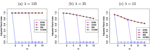
Figure 1: Results for the degree-corrected stochastic block model with two values for the degree parameters, $\pi=0.5$, $m$ varies.

Figure 1 shows the results for three different expected degrees $\lambda$. For the densest network with $\lambda=125$ in Figure 1(a), the degree-corrected block model and Newman–Girvan modularity perform the best overall, as they assume the correct model and the methods are consistent. At $m=1$, the regular block model is just as good, but its performance deteriorates rapidly as $m$ increases. The Erdos–Renyi modularity also performs perfectly for $m=1$, and it takes larger values of $m$ for its performance to deteriorate than for block model likelihood, so we can conclude that the Erdos–Renyi modularity is more robust to variation in degrees. For both of them, poor results are due to grouping nodes with similar degrees together. The overall trend for sparser networks [Figure 1(b) and (c)] is similar, but all methods perform worse, as with fewer links there is effectively less data to use for fitting the model, and the effect is more pronounced for large $m$, when degrees have higher variance.

Figure 2: Results for the standard stochastic block model, $m=1$, $\pi$ varies.

5.2 The stochastic block model

Here we focus on the standard stochastic block model ($m=1$) and vary $\pi$ to assess robustness to unbalanced community sizes. All the four criteria are consistent in this case, but, in practice, the closer $\pi$ is to 0.5, the better they perform (Figure 2), with the exception of the block model likelihood in the dense case ($\lambda=125$), where it performs perfectly for all $\pi$. Overall, the block model likelihood performs best, which is natural because it is the maximum likelihood estimator of the correct model. The Erdos–Renyi modularity also performs better than the other two criteria, which overfit the data by assuming the degree-corrected model and accounting for variation in observed degrees, which in this case only adds noise.

5.3 Unbalanced community sizes

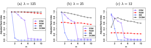
Figure 3: Results for the degree-corrected stochastic block model with two values for the degree parameters, $\pi=0.3$, $m$ varies.

In this simulation we consider the degree-corrected stochastic block model with unbalanced community sizes. We fix $\pi=0.3$ and vary the ratio $m$ in Figure 3. For a dense network [$\lambda=125$, Figure 3(a)], the performance with $\pi=0.3$ is similar to the balanced case with $\pi=0.5$ [Figure 1(a)]. However, in sparser networks modularity performs much worse with unbalanced community sizes. This can also be seen in Figure 2 for the case $m=1$. The failure of modularity to deal with unbalanced community sizes was also recently pointed out by Zhang&Zhao2012 . Note also that in the sparsest case ($\lambda=12$, Figure 3), the degree-corrected model suffers from over-fitting when $m=1$, as was also seen in Figure 2.

5.4 A different degree distribution

In the last simulation we test the sensitivity of all methods, but in particular the degree-corrected model, to the assumption of a discrete degree distribution. Here we sample the degree parameters $\theta_{i}$ independently from the following distribution:

$$\theta_{i}=\cases{\eta_{i},&\quad$\mbox{w.p. $\alpha$,}$\vspace*{2pt}\cr 2/(m+1),&\quad$\mbox{w.p. $(1-\alpha)/2$,}$\vspace*{2pt}\cr 2m/(m+1),&\quad$\mbox{w.p. $(1-\alpha)/2$,}$}$$

where $\eta_{i}$ is uniformly distributed on the interval $[0,2]$. The variance of $\theta_{i}$ is equal to $\alpha/3+(1-\alpha)(m-1)^{2}/(m+1)^{2}$. In this simulation, we fix $m=10$, which makes the variance a decreasing function of $\alpha$, and vary $\alpha$ from 0 to 1. We also fix $\pi=0.5$.

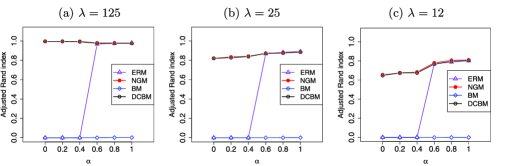
Figure 4: Results for the degree-corrected stochastic block model with a mixture degree distribution, $m=10$, $\pi=0.5$, mixture parameter $\alpha$ varies.

The results in Figure 4 show that the degree-corrected block model likelihood and Newman–Girvan modularity still perform well, which suggests that the discreteness of $\theta$ is not a crucial assumption. The regular block model fails in this case, as we would expect from earlier results since $m=10$, but the performance of the Erdos–Renyi modularity improves as $\alpha$ increases, which agrees with our earlier observation on its relative robustness to variation in degrees.

6 Example: The political blogs network

In this section we analyze a real network of political blogs compiled by Adamic05 . The nodes of this network are blogs about US politics and the edges are hyperlinks between these blogs. The data were collected right after the 2004 presidential election and demonstrate strong divisions; each blog was manually labeled as liberal or conservative by Adamic05 , which we take as ground truth. Following the analysis in Karrer10 , we ignore directions of the hyperlinks and focus on the largest connected component of this network, which contains 1222 nodes, 16,714 edges and has the average degree of approximately 27. Some summary statistics of the node degrees are given in Table 2, which shows that the degree distribution is heavily skewed to the right.

Table 2: Statistics of node degrees in the political blogs network

Mean	Median	Min	1st Qt.	3rd Qt.	Max
27.36	13.00	1.00	3.00	36.00	351.00

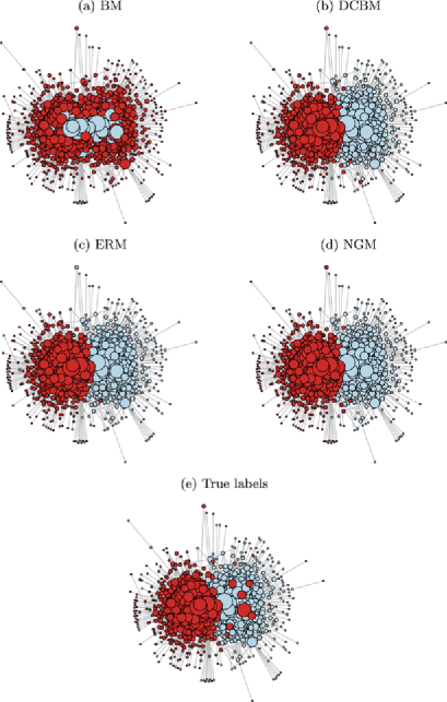
Figure 5: Political blogs data. Node area is proportional to the logarithm of its degree and the colors represent community labels.

We compare the partitions into two communities found by the four different community detection criteria with the true labels using the adjusted Rand index. The Newman–Girvan modularity and the degree-corrected model find very similar partitions (they differ over only four nodes and have the same adjusted Rand index value of 0.819, the highest of all methods). The partition found by the Erdos–Renyi modularity has a slightly worse agreement with the truth (adjusted Rand index of 0.793). The block model likelihood divides the nodes into two groups of low degree and high degree, with the adjusted Rand index of nearly 0, which is equivalent to random guessing. The results are shown in Figure 5 (drawn using the igraph package in R igraph with the Fruchterman and Reingold layout Fruchterman1991 ). These are consistent with what we observed in simulation studies: the Newman–Girvan modularity and the degree-corrected block model likelihood perform better in a network with high degree variation, and the Erdos–Renyi modularity is more robust to degree variation than the block model likelihood.

All criteria were maximized by tabu search, but for modularities we also computed the solutions based on the eigendecomposition of the modularity matrix. Both solutions were worse that those found by tabu search, but while for Newman–Girvan modularity the difference was slight (the adjusted Rand index of 0.781 instead of 0.819), eigendecomposition of the Erdos–Renyi modularity yielded a poor result similar to that of block model likelihood (with adjusted Rand index value of 0.092 instead of 0.819 by tabu search). This suggests that Erdos–Renyi modularity is numerically less stable under high degree variation, in addition to being theoretically not consistent. More analysis of the eigendecomposition-based solutions is needed for both types of modularities to understand conditions under which these approximations work well.

7 Summary and discussion

In this paper we developed a general tool for checking consistency of community detection criteria under the degree-corrected stochastic block model, a more general and practical model than the standard stochastic block model for which such theory was previously available Bickel&Chen2009 . This general tool allowed us to obtain consistency results for four different community detection criteria, and, to the best of our knowledge for the first time in the networks literature, to clearly separate the effects of the model assumed for criteria derivation from the model assumed true for analysis of the criteria. What we have shown is, essentially, statistical common sense: methods are consistent when the model they assume holds for the data. The parameter constraints are needed when methods implicitly rely on them, although we found that the two different modularity methods, while using the same constraint in spirit, require somewhat different conditions on parameters to be consistent. The theoretical analysis agrees well with both simulation studies and the data analysis, which also indicate that the methods with better theoretical consistency properties do not always perform best in practice: there is a cost associated with fitting the extra complexity of the degree-corrected model, and if there is not enough data for that, or the data does not have much variation in node degrees, simpler methods based on the standard stochastic block model will in fact do better.

There are many questions that require further investigation here, even in the context of model-based community detection when a model is assumed true. For example, we assumed that $K$ is known, which is not unreasonable in some cases (e.g., dividing political blogs into liberal and conservative), but is in general a difficult open problem in community detection. Standard methods such as AIC and BIC do not seem to lend themselves easily to this case, because of parameters disappearing in nonstandard ways when going from $K+1$ to $K$ blocks. A permutation test was proposed in Zhaoetal2011 , but clearly more work is needed. There is also the question of what happens if $K$ is allowed to grow with $n$, which is probably more realistic than fixed $K$; for the stochastic block model, this case has been considered by Choietal2011 and Rohe2011 , but their analysis is specific to the particular methods they considered and does not extend easily to the degree-corrected block model. Another open question is the properties of approximate but more easily computable solutions based on the eigendecomposition, as opposed to the properties of global maximizers we studied here. For the stochastic block model, part of this analysis was performed in Rohe2011 . Our practical experience suggests that the behavior of eigenvectors can be quite complicated, and it is not understood at this point when this approximation works well. Finally, the sparse case $\lambda_{n}=O(1)$ is an open problem in general, although results for some special cases of the stochastic block model have been recently obtained coja09 , Decelleetal2011 .

Appendix

We start from summarizing notation. Let $R(\mathbf{e}),V(\mathbf{e})\in\mathcal{R}^{K\times K\times M}$, $\hat{\Pi}\in\mathcal{R}^{K\times M}$, $f(\mathbf{e}),f^{0}(\mathbf{e})\in\mathcal{R}^{K}$, where

$$R_{kau}(\mathbf{e}) = \frac{1}{n}\sum_{i=1}^{n}I(e_{i}=k,c_{i}=a,\theta_{i}=x_{u}),$$

$$V_{kau}(\mathbf{e}) = \frac{\sum_{i=1}^{n}I(e_{i}=k,c_{i}=a,\theta_{i}=x_{u})}{\sum_{i=1}^{n}I(c_{i}=a,\theta_{i}=x_{u})},$$

$$\hat{\Pi}_{au} = \frac{1}{n}\sum_{i=1}^{n}I(c_{i}=a,\theta_{i}=x_{u}),$$

$$f_{k}(\mathbf{e}) = \frac{1}{n}\sum_{i=1}^{n}I(e_{i}=k)=\sum_{au}V_{kau}(\mathbf{e})\hat{\Pi}_{au},$$

$$f^{0}_{k}(\mathbf{e}) = \sum_{au}V_{kau}(\mathbf{e})\Pi_{au}.$$

Even though the arbitrary labeling $\mathbf{e}$ is not random, intuitively one can think of $R$ as the empirical joint distribution of $\mathbf{e}$, $\mathbf{c}$, and $\bolds{\theta}$, $V$ as the conditional distribution of $\mathbf{e}$ given $\mathbf{c}$ and $\bolds{\theta}$. Further, $\hat{\Pi}$ is the empirical joint distribution of $\mathbf{c}$ and $\bolds{\theta}$, and thus an estimate of their true joint distribution $\Pi$, $f$ is the empirical marginal “distribution” of $\mathbf{e}$, and $f^{0}$ is the same marginal but with the empirical joint distribution $\hat{\Pi}$ replaced by its population version $\Pi$. Then $\sum_{k}V_{kau}(\mathbf{e})=1$, and $V_{kau}(\mathbf{c})=I(k=a)$ for all $u$. Further, define $\hat{T}(\mathbf{e})\in\mathcal{R}^{K\times K}$ to be a rescaled expectation of the matrix $O$ conditional on $c$ and $\theta$,

$$\hat{T}_{kl}(\mathbf{e})=\frac{1}{\mu_{n}}\mathbb{E}[O_{kl}|\mathbf{c},\bolds{\theta}].$$

From Proposition 4.1,

$$\hat{T}_{kl}(\mathbf{e}) = \sum_{abuv}x_{u}x_{v}P_{ab}R_{kau}(\mathbf{e})R_{lbv}(\mathbf{e})$$

$$= \sum_{abuv}x_{u}x_{v}P_{st}V_{kau}(\mathbf{e})\hat{\Pi}_{au}V_{lbv}(\mathbf{e})\hat{\Pi}_{bv}.$$

Replacing $\hat{\Pi}$ by its expectation $\hat{\Pi}$, we define $T(\mathbf{e})\in\mathcal{R}^{K\times K}$ by

$$T_{kl}(\mathbf{e})=\sum_{abuv}x_{u}x_{v}P_{st}V_{kau}(\mathbf{e})\Pi_{au}V_{lbv}(\mathbf{e})\Pi_{bv}.$$

Also define $X(\mathbf{e})\in\mathcal{R}^{K\times K}$ to be the rescaled difference between $O$ and its conditional expectation,

$$X_{kl}(\mathbf{e})=\frac{O_{kl}(\mathbf{e})}{\mu_{n}}-\hat{T}_{kl}(\mathbf{e}).$$

These quantities will be used in the proof of the general Theorem 4.1, where we first approximate $\frac{1}{\mu_{n}}O_{kl}$ by $\hat{T}_{kl}(\mathbf{e})$ and then approximate $\hat{T}_{kl}(\mathbf{e})$ by $T_{kl}(\mathbf{e})$.

Proof of Proposition 4.1 We only proof (11) since (12) is trivial.

$$\frac{1}{\mu_{n}}\mathbb{E}[O_{kl}|\mathbf{c},\bolds{\theta}]$$

$$\qquad=\frac{1}{\mu_{n}}\sum_{ij}\sum_{abuv}\mathbb{E}\bigl{[}A_{ij}I(e_{i}=k,c_{i}=a,\theta_{i}=x_{u})I(e_{j}=l,c_{j}=b,\theta_{j}=x_{v})|\mathbf{c},\bolds{\theta}\bigr{]}$$

$$\qquad=\sum_{abuv}x_{u}x_{v}P_{ab}R_{kau}(\mathbf{e})R_{lbv}(\mathbf{e})=H_{kl}\bigl{(}R(\mathbf{e})\bigr{)}.$$

Before we proceed to the general theorem, we state a lemma based on Bernstein’s inequality.

Lemma .1

Let $\|X\|_{\infty}=\max_{kl}|X_{kl}|$ and $|\mathbf{e}-\mathbf{c}|=\sum_{i=1}^{n}I(e_{i}\neq c_{i})$. Then

$$\mathbb{P}\Bigl{(}\max_{\mathbf{e}}\bigl{\|}X(\mathbf{e})\bigr{\|}_{\infty}\geq\varepsilon\Bigr{)}\leq 2K^{n+2}\exp\biggl{(}-\frac{1}{8C}\varepsilon^{2}\mu_{n}\biggr{)}$$ (13)

for $\varepsilon<3C$, where $C=\max\{x_{u}x_{v}P_{ab}\}$.

$$\quad\mathbb{P}\Bigl{(}\max_{|\mathbf{e}-\mathbf{c}|\leq m}\bigl{\|}X(\mathbf{e})-X(\mathbf{c})\bigr{\|}_{\infty}\geq\varepsilon\Bigr{)}\leq 2\pmatrix{{n}\cr{m}}K^{m+2}\exp\biggl{(}-\frac{3}{8}\varepsilon\mu_{n}\biggr{)}$$ (14)

for $\varepsilon\geq 6Cm/n$.

$$\mathbb{P}\Bigl{(}\max_{|\mathbf{e}-\mathbf{c}|\leq m}\bigl{\|}X(\mathbf{e})-X(\mathbf{c})\bigr{\|}_{\infty}\geq\varepsilon\Bigr{)}\leq 2\pmatrix{{n}\cr{m}}K^{m+2}\exp\biggl{(}-\frac{n}{16mC}\varepsilon^{2}\mu_{n}\biggr{)}$$ (15)

for $\varepsilon<6Cm/n$.

This lemma is similar to Lemma 1.1 of Bickel&Chen2009 , with a few minor errors corrected. The proof can be found in the electronic supplement to this article Zhaoetal-aossupp . Proof of Theorem 4.1 The proof is divided into three steps.

Step 1: show that $F(\frac{O(\mathbf{e})}{\mu_{n}},f(\mathbf{e}))$ is uniformly close to its population version. More precisely, we need to prove that there exists $\varepsilon_{n}\rightarrow 0$, such that

$$\qquad\mathbb{P}\biggl{(}\max_{\mathbf{e}}\biggl{|}F\biggl{(}\frac{O(\mathbf{e})}{\mu_{n}},f(\mathbf{e})\biggr{)}-F\bigl{(}T(\mathbf{e}),f^{0}(\mathbf{e})\bigr{)}\biggr{|}<\varepsilon_{n}\biggr{)}\rightarrow 1\qquad\mbox{if }\lambda_{n}\rightarrow\infty.$$ (16)

Since

$$\biggl{|}F\biggl{(}\frac{O(\mathbf{e})}{\mu_{n}},f(\mathbf{e})\biggr{)}-F\bigl{(}T(\mathbf{e}),f^{0}(\mathbf{e})\bigr{)}\biggr{|} \leq \biggl{|}F\biggl{(}\frac{O(\mathbf{e})}{\mu_{n}},f(\mathbf{e})\biggr{)}-F\bigl{(}\hat{T}(\mathbf{e}),f(\mathbf{e})\bigr{)}\biggr{|}$$

$${}+\bigl{|}F\bigl{(}\hat{T}(\mathbf{e}),f(\mathbf{e})\bigr{)}-F\bigl{(}T(\mathbf{e}),f^{0}(\mathbf{e})\bigr{)}\bigr{|},$$

it is sufficient to bound these two terms uniformly. By Lipschitz continuity,

$$\biggl{|}F\biggl{(}\frac{O(\mathbf{e})}{\mu_{n}},f(\mathbf{e})\biggr{)}-F\bigl{(}\hat{T}(\mathbf{e}),f(\mathbf{e})\bigr{)}\biggr{|}\leq M_{1}\bigl{\|}X(e)\bigr{\|}_{\infty}.$$ (17)

By (13), (17) converges to 0 uniformly if $\lambda_{n}\rightarrow\infty$, and

$$\bigl{|}F\bigl{(}\hat{T}(\mathbf{e}),f(\mathbf{e})\bigr{)}-F\bigl{(}T(\mathbf{e}),f^{0}(\mathbf{e})\bigr{)}\bigr{|}$$

(18)

$$\qquad\leq M_{1}\bigl{\|}\hat{T}(\mathbf{e})-T(\mathbf{e})\bigr{\|}_{\infty}+M_{2}\bigl{\|}f(\mathbf{e})-f^{0}(\mathbf{e})\bigr{\|}$$

where $\|\cdot\|$ is the Euclidean norm for vectors. Further,

$$\bigl{|}\hat{T}_{kl}(\mathbf{e})-T_{kl}(\mathbf{e})\bigr{|} = \biggl{|}\sum_{abuv}x_{u}x_{v}P_{ab}V_{kau}(\mathbf{e})V_{lbv}(\mathbf{e})(\hat{\Pi}_{au}\hat{\Pi}_{bv}-\Pi_{au}\Pi_{bv})\biggr{|}$$

$$\leq \sum_{abuv}x_{u}x_{v}P_{ab}|\hat{\Pi}_{au}\hat{\Pi}_{bv}-\Pi_{au}\Pi_{bv}|,$$

and

$$\bigl{|}f_{k}(\mathbf{e})-f^{0}_{k}(\mathbf{e})\bigr{|}=\biggl{|}\sum_{au}V_{kau}(\mathbf{e})(\hat{\Pi}_{au}-\Pi_{au})\biggr{|}\leq\sum_{au}|\hat{\Pi}_{au}-\Pi_{au}|.$$ (20)

Since $\hat{\Pi}\stackrel{{\scriptstyle P}}{{\rightarrow}}\Pi$, (Appendix) converges to 0 uniformly. Thus, (16) holds.

Step 2: Prove that there exists $\delta_{n}\rightarrow 0$, such that

$$\mathbb{P}\biggl{(}\max_{\{\mathbf{e}\dvtx\|V(\mathbf{e})-\mathbb{I}\|_{1}\geq\delta_{n}\}}F\biggl{(}\frac{O(\mathbf{e})}{\mu_{n}},f(\mathbf{e})\biggr{)}<F\biggl{(}\frac{O(\mathbf{c})}{\mu_{n}},f(\mathbf{c})\biggr{)}\biggr{)}\rightarrow 1,$$ (21)

where $\|W\|_{1}=\sum_{kau}|W_{kau}|$ for $W\in\mathcal{R}^{K\times K\times M}$.

By continuity and ($\ast$), there exists $\delta_{n}\rightarrow 0$, such that

$$F\bigl{(}T(\mathbf{c}),f^{0}(\mathbf{c})\bigr{)}-F\bigl{(}T(\mathbf{e}),f^{0}(\mathbf{e})\bigr{)}>2\varepsilon_{n}$$

if $\|V(\mathbf{e})-\mathbb{I}\|_{1}\geq\delta_{n}$, where $\mathbb{I}=V(\mathbf{c})$. Thus, from (16),

$$\mathbb{P}\biggl{(}\max_{\{\mathbf{e}\dvtx\|V(\mathbf{e})-\mathbb{I}\|_{1}\geq\delta_{n}\}}F\biggl{(}\frac{O(\mathbf{e})}{\mu_{n}},f(\mathbf{e})\biggr{)}<F\biggl{(}\frac{O(\mathbf{c})}{\mu_{n}},f(\mathbf{c})\biggr{)}\biggr{)}$$

$$\qquad\geq\mathbb{P}\biggl{(}\biggl{|}\max_{\{\mathbf{e}\dvtx\|V(\mathbf{e})-\mathbb{I}\|_{1}\geq\delta_{n}\}}F\biggl{(}\frac{O(\mathbf{e})}{\mu_{n}},f(\mathbf{e})\biggr{)}$$

$$\hskip 27.0pt\qquad{}-\max_{\{\mathbf{e}\dvtx\|V(\mathbf{e})-\mathbb{I}\|_{1}\geq\delta_{n}\}}F\bigl{(}T(\mathbf{e}),f^{0}(\mathbf{e})\bigr{)}\biggr{|}<\varepsilon_{n},$$

$$\hskip 46.0pt\biggl{|}F\biggl{(}\frac{O(\mathbf{c})}{\mu_{n}},f(\mathbf{c})\biggr{)}-F\bigl{(}T(\mathbf{c}),f^{0}(\mathbf{c})\bigr{)}\biggr{|}<\varepsilon_{n}\biggr{)}\rightarrow 1.$$

(21) implies

$$\mathbb{P}\bigl{(}\bigl{\|}V(\hat{c})-\mathbb{I}\bigr{\|}<\delta_{n}\bigr{)}\rightarrow 1.$$

Since

$$\frac{1}{n}|\mathbf{e}-\mathbf{c}| = \frac{1}{n}\sum_{i=1}^{n}I(c_{i}\neq e_{i})=\sum_{au}\Pi_{au}\bigl{(}1-V_{aau}(\mathbf{e})\bigr{)}\leq\sum_{au}\bigl{(}1-V_{aau}(\mathbf{e})\bigr{)}$$

$$= \frac{1}{2}\biggl{(}\sum_{au}\bigl{(}1-V_{aau}(\mathbf{e})\bigr{)}+\sum_{au}\sum_{k\neq a}V_{kau}(\mathbf{e})\biggr{)}=\frac{1}{2}\bigl{\|}V(\mathbf{e})-\mathbb{I}\bigr{\|}_{1},$$

weak consistency follows.

Step 3: In order to prove strong consistency, we need to show that

$$\mathbb{P}\biggl{(}\max_{\{\mathbf{e}\dvtx 0<\|V(\mathbf{e})-\mathbb{I}\|_{1}<\delta_{n}\}}F\biggl{(}\frac{O(\mathbf{e})}{\mu_{n}},f(\mathbf{e})\biggr{)}<F\biggl{(}\frac{O(\mathbf{c})}{\mu_{n}},f(\mathbf{c})\biggr{)}\biggr{)}\rightarrow 1.$$ (22)

Note that combining (21) and (22), we have

$$\mathbb{P}\biggl{(}\max_{\{\mathbf{e}\dvtx\mathbf{e}\neq\mathbf{c}\}}F\biggl{(}\frac{O(\mathbf{e})}{\mu_{n}},f(\mathbf{e})\biggr{)}<F\biggl{(}\frac{O(\mathbf{c})}{\mu_{n}},f(\mathbf{c})\biggr{)}\biggr{)}\rightarrow 1,$$

which implies the strong consistency.

Here we closely follow the derivation given in AiroldiNotes . To prove (22), note that by Lipschitz continuity and the continuity of derivatives of $F$ with respect to $V(\mathbf{e})$ in the neighborhood of $\mathbb{I}$, we have

$$F\biggl{(}\frac{O(\mathbf{e})}{\mu_{n}},f(\mathbf{e})\biggr{)}-F\biggl{(}\frac{O(\mathbf{c})}{\mu_{n}},f(\mathbf{c})\biggr{)}$$

(23)

$$\qquad=F\bigl{(}\hat{T}(\mathbf{e}),f(\mathbf{e})\bigr{)}-F\bigl{(}\hat{T}(\mathbf{c}),f(\mathbf{c})\bigr{)}+\Delta(\mathbf{e},\mathbf{c}),$$

where $|\Delta(\mathbf{e},\mathbf{c})|\leq M^{\prime}(\|X(\mathbf{e})-X(\mathbf{c})\|_{\infty})$, and

$$F\bigl{(}T(\mathbf{e}),f^{0}(\mathbf{e})\bigr{)}-F\bigl{(}T(\mathbf{c}),f^{0}(\mathbf{c})\bigr{)}$$

(24)

$$\qquad\leq-C^{\prime}\bigl{\|}V(\mathbf{e})-\mathbb{I}\bigr{\|}_{1}+o\bigl{(}\bigl{\|}V(\mathbf{e})-\mathbb{I}\bigr{\|}_{1}\bigr{)}.$$

Since the derivative of $F$ is continuous with respect to $V(\mathbf{e})$ in the neighborhood of $\mathbb{I}$, there exists a $\delta^{\prime}$ such that

$$F\bigl{(}\hat{T}(\mathbf{e}),f(\mathbf{e})\bigr{)}-F\bigl{(}\hat{T}(\mathbf{c}),f(\mathbf{c})\bigr{)}$$

(25)

$$\qquad\leq-\bigl{(}C^{\prime}/2\bigr{)}\bigl{\|}V(\mathbf{e})-\mathbb{I}\bigr{\|}_{1}+o\bigl{(}\bigl{\|}V(\mathbf{e})-\mathbb{I}\bigr{\|}_{1}\bigr{)}$$

holds when $\|\hat{\Pi}-\Pi\|_{\infty}\leq\delta^{\prime}$. Since $\hat{\Pi}\rightarrow\Pi$, (Appendix) holds with probability approaching 1. Combining (Appendix) and (Appendix), it is easy to see that (22) follows if we can show

$$\mathbb{P}\Bigl{(}\max_{\{\mathbf{e}\neq\mathbf{c}\}}\bigl{|}\Delta(\mathbf{e},\mathbf{c})\bigr{|}\leq C^{\prime}\bigl{\|}V(\mathbf{e})-\mathbb{I}\bigr{\|}_{1}/4\Bigr{)}\rightarrow 1.$$ (26)

Again note that $\frac{1}{n}|\mathbf{e}-\mathbf{c}|\leq\frac{1}{2}\|V(\mathbf{e})-\mathbb{I}\|_{1}$. So for each $m\geq 1$,

$$\mathbb{P}\Bigl{(}\max_{|\mathbf{e}-\mathbf{c}|=m}\bigl{|}\Delta(\mathbf{e},\mathbf{c})\bigr{|}>C^{\prime}\bigl{\|}V(\mathbf{e})-\mathbb{I}\bigl{\|}_{1}/4\Bigr{)}$$

(27)

$$\qquad\leq\mathbb{P}\biggl{(}\max_{|\mathbf{e}-\mathbf{c}|\leq m}\bigl{\|}X(\mathbf{e})-X(\mathbf{c})\bigr{\|}_{\infty}>\frac{C^{\prime}m}{2M^{\prime}n}\biggr{)}=I_{1}.$$

Let $\alpha=C^{\prime}/2M^{\prime}$, if $\alpha\geq 6C$, by (14),

$$I_{1} \leq 2K^{m+2}n^{m}\exp\biggl{(}-\alpha\frac{3m}{8n}\mu_{n}\biggr{)}$$

$$= 2K^{2}\bigl{[}K\exp\bigl{(}\log n-\alpha\mu_{n}/(8/3n)\bigr{)}\bigr{]}^{m}.$$

If $\alpha<6C$, by (15),

$$I_{1} \leq 2K^{m+2}n^{m}\exp\biggl{(}-\alpha^{2}\frac{m}{16Cn}\mu_{n}\biggr{)}$$

$$= 2K^{2}\bigl{[}K\exp\bigl{(}\log n-\alpha^{2}\mu_{n}/(16Cn)\bigr{)}\bigr{]}^{m}.$$

In both cases, since $\lambda_{n}/\log n\rightarrow\infty$,

$$\mathbb{P}\Bigl{(}\max_{\{\mathbf{e}\neq\mathbf{c}\}}\bigl{|}\Delta(\mathbf{e},\mathbf{c})\bigr{|}>C^{\prime}\bigl{\|}V(\mathbf{e})-\mathbb{I}\bigr{\|}_{1}/4\Bigr{)}$$

$$\qquad=\sum_{m=1}^{\infty}\mathbb{P}\Bigl{(}\max_{|\mathbf{e}-\mathbf{c}|=m}\bigl{|}\Delta(\mathbf{e},\mathbf{c})\bigr{|}>C^{\prime}\bigl{\|}V(\mathbf{e})-\mathbb{I}\bigr{\|}_{1}/4\Bigr{)}\rightarrow 0$$

as $n\rightarrow\infty$, which completes the proof.

Proof of Theorem 3.2 The regularity conditions are easy to verify. To check the key condition ($\ast$), note that under the block model assumption, ($\ast$) becomes

• [($\ast\ast$)]

• $F(H(S),h(S))$ is uniquely maximized over $\mathscr{S}=\{S\dvtx S\geq 0,\sum_{k}S_{ka}=\pi_{a}\}$ by $S=D$, with $D=\operatorname{diag}(\bolds{\pi})$,

where $S$ is a generic $K$ by $K$ matrix.

Up to a constant, the population version of $Q_{\mathrm{ERM}}$ is

$$F\bigl{(}H(S),h(S)\bigr{)}=\sum_{k}\bigl{(}H_{kk}-h_{k}^{2}P_{0}\bigr{)}.$$

Using the identity,

$$\sum_{k}\bigl{(}H_{kk}-h_{k}^{2}P_{0}\bigr{)}+\sum_{k\neq l}(H_{kl}-h_{k}h_{l}P_{0})=\sum_{kl}H_{kl}-\biggl{(}\sum_{k}h_{k}\biggr{)}^{2}P_{0}=0,$$

and define

$$\Delta_{kl}=\cases{1,&\quad$\mbox{if $k=l$}$,\vspace*{2pt}\cr-1,&\quad$\mbox{if $k\neq l$.}$}$$

Then we have

$$F\bigl{(}H(S),h(S)\bigr{)} = \frac{1}{2}\sum_{kl}\Delta_{kl}(H_{kl}-h_{k}h_{l}P_{0})$$

$$= \frac{1}{2}\sum_{kl}\Delta_{kl}\biggl{(}\sum_{ab}S_{ka}S_{lb}P_{ab}-\sum_{ab}S_{ka}S_{lb}P_{0}\biggr{)}$$

$$= \frac{1}{2}\sum_{kl}\sum_{ab}S_{ka}S_{lb}\Delta_{kl}(P_{ab}-P_{0})$$

$$\leq \frac{1}{2}\sum_{kl}\sum_{ab}S_{ka}S_{lb}\Delta_{ab}(P_{ab}-P_{0})$$

$$= \frac{1}{2}\sum_{ab}\Delta_{ab}\pi_{a}\pi_{b}(P_{ab}-P_{0})=F\bigl{(}H(D),h(D)\bigr{)}.$$

Now it remains to show the diagonal matrix $D$ (up to a permutation) is the unique maximizer of $F$. This follows from Lemma 3.2 in Bickel&Chen2009 , since equality holds only if $\Delta_{kl}=\Delta_{ab}$ when $S_{ka}S_{lb}>0$ and $\Delta$ does not have two identical columns.

Proof of Theorem 3.1 The consistency of Newman–Girvan modularity under the block model has already been shown in Bickel&Chen2009 . To extend this result to the degree-corrected block model, define $\tilde{S}_{ka}=\sum_{u}x_{u}S_{kau}$. Then

$$\tilde{\pi}_{a} = \sum_{k}\tilde{S}_{ka},$$

$$H_{kl} = \sum_{abuv}x_{u}x_{v}P_{ab}S_{kau}S_{lbv}=\sum_{ab}\tilde{S}_{ka}\tilde{S}_{lb}P_{ab},$$

$$H_{k} = \sum_{l}H_{kl}=\sum_{as}\tilde{S}_{ka}\tilde{\pi}_{s}P_{as}.$$

The population version of $Q_{\mathrm{NGM}}$ is

$$F\bigl{(}H(S)\bigr{)}=\sum_{k}\biggl{(}\frac{H_{kk}}{\tilde{P}_{0}}-\biggl{(}\frac{H_{k}}{\tilde{P}_{0}}\biggr{)}^{2}\biggr{)}.$$

Using the identity

$$\sum_{k}\biggl{(}\frac{H_{kk}}{\tilde{P}_{0}}-\biggl{(}\frac{H_{k}}{\tilde{P}_{0}}\biggr{)}^{2}\biggr{)}+\sum_{k\neq l}\biggl{(}\frac{H_{kl}}{\tilde{P}_{0}}-\frac{H_{k}H_{l}}{\tilde{P}_{0}^{2}}\biggr{)}=\sum_{kl}\frac{H_{kl}}{\tilde{P}_{0}}-\biggl{(}\sum_{k}\frac{H_{k}}{\tilde{P}_{0}}\biggr{)}^{2}=0,$$

we obtain

$$F\bigl{(}H(S)\bigr{)} = \frac{1}{2}\sum_{kl}\Delta_{kl}\biggl{(}\frac{\sum_{ab}\tilde{S}_{ka}\tilde{S}_{lb}P_{ab}}{\tilde{P}_{0}}-\frac{(\sum_{as}\tilde{S}_{ka}\tilde{\pi}_{s}P_{as})(\sum_{bt}\tilde{S}_{lb}\tilde{\pi}_{t}P_{bt})}{\tilde{P}_{0}^{2}}\biggr{)}$$

$$= \frac{1}{2}\sum_{kl}\sum_{ab}\tilde{S}_{ka}\tilde{S}_{lb}\Delta_{kl}\biggl{(}\frac{P_{ab}}{\tilde{P}_{0}}-\frac{(\sum_{s}\tilde{\pi}_{s}P_{as})(\sum_{t}\tilde{\pi}_{t}P_{bt})}{\tilde{P}_{0}^{2}}\biggr{)}$$

$$\leq \frac{1}{2}\sum_{kl}\sum_{ab}\tilde{S}_{ka}\tilde{S}_{lb}\Delta_{ab}\biggl{(}\frac{P_{ab}}{\tilde{P}_{0}}-\frac{(\sum_{s}\tilde{\pi}_{s}P_{as})(\sum_{t}\tilde{\pi}_{t}P_{bt})}{\tilde{P}_{0}^{2}}\biggr{)}$$

$$= \frac{1}{2}\sum_{ab}\Delta_{ab}\tilde{\pi}_{a}\tilde{\pi}_{b}\biggl{(}\frac{P_{ab}}{\tilde{P}_{0}}-\frac{(\sum_{s}\tilde{\pi}_{s}P_{as})(\sum_{t}\tilde{\pi}_{t}P_{bt})}{\tilde{P}_{0}^{2}}\biggr{)}=F\bigl{(}H(\mathbb{D})\bigr{)}.$$

Similar to Theorem 3.2, $D$ is the unique maximizer of $F(H(\tilde{S}))$, so it is enough to show $S=\mathbb{D}$ whenever $\tilde{S}=D$ to prove uniqueness. $\tilde{S}=D$ implies $\tilde{S}_{ka}=0$, if $k\neq a$. Since $x_{u}>0$, we obtain $S_{kau}=0$ if $k\neq a$, which gives the result.

We note that this argument cannot be applied to prove the consistency of Erdos–Renyi modularity under degree-corrected block models, because in that case $h_{k}=\sum_{au}S_{kau}\neq\sum_{a}(\sum_{u}x_{u}S_{kau})=\sum_{a}\tilde{S}_{ka}$, when we use the transformation $\tilde{S}_{ka}=\sum_{u}x_{u}S_{kau}$.

Proof of Theorem 3.4 Up to a constant, the population version of $Q_{\mathrm{BL}}$ is

$$F\bigl{(}H(S),h(S)\bigr{)}=\sum_{kl}\biggl{(}H_{kl}\log\frac{H_{kl}}{h_{k}h_{l}}-H_{kl}\biggr{)}.$$

Let $g_{kl}=H_{kl}/(h_{k}h_{l})$,

$$F\bigl{(}H(S),h(S)\bigr{)} = \sum_{kl}(H_{kl}\log g_{kl}-h_{k}h_{l}g_{kl})=\sum_{abkl}S_{ka}S_{lb}(P_{ab}\log g_{kl}-g_{kl})$$

$$\leq \sum_{ab}\sum_{kl}S_{ka}S_{lb}(P_{ab}\log P_{ab}-P_{ab})$$

$$= \sum_{ab}(\pi_{a}\pi_{b}P_{ab}\log P_{ab}-\pi_{a}\pi_{b}P_{ab})=F\bigl{(}H(D),h(D)\bigr{)}.$$

Since the inequality holds if and only if $g_{kl}=P_{ab}$ when $S_{ka}S_{lb}>0$, uniqueness follows from Lemma .2, stated next.

Lemma .2

Let $g$, $P$, $S$ be $K\times K$ matrices with nonnegative entries. Assume that: [(a)]

$P$ and $g$ are symmetric;

$P$ does not have two identical columns;

there exists at least one nonzero entry in each column of $S$;

for $1\leq k,l,a,b\leq K,g_{kl}=P_{ab}$ whenever $S_{ka}S_{lb}>0$. Then $S$ is a diagonal matrix or a row/column permutation of a diagonal matrix.

This lemma is a generalization of Lemma 3.2 in Bickel&Chen2009 . The proof is given in the electronic supplement Zhaoetal-aossupp . Proof of Theorem 3.3 Up to a constant, the population version of $Q_{\mathrm{DCBM}}$ is

$$F\bigl{(}H(S)\bigr{)}=\sum_{kl}\biggl{(}H_{kl}\log\frac{H_{kl}}{H_{k}H_{l}}-H_{kl}\biggr{)},$$ (28)

where we only check ($\ast\ast$) [the form ($\ast$) takes under the block model]. The generalization to the degree-corrected block model is similar to the proof of Theorem 3.1 and is omitted.

Let $g_{kl}=H_{kl}/(H_{k}H_{l})$, and

$$F\bigl{(}H(S)\bigr{)} = \sum_{kl}(H_{kl}\log g_{kl}-H_{k}H_{l}g_{kl})$$

$$= \sum_{kl}\biggl{[}\sum_{ab}S_{ka}S_{lb}P_{ab}\log g_{kl}-\biggl{(}\sum_{as}S_{ka}\pi_{s}P_{as}\biggr{)}\biggl{(}\sum_{bt}\pi_{t}S_{lb}P_{tb}\biggr{)}g_{kl}\biggr{]}$$

$$= \sum_{kl}\sum_{ab}S_{ka}S_{lb}\biggl{[}P_{ab}\log g_{kl}-\biggl{(}\sum_{s}\pi_{s}P_{as}\biggr{)}\biggl{(}\sum_{t}\pi_{t}P_{tb}\biggr{)}g_{kl}\biggr{]}=I_{2}.$$

Since $\operatorname{arg\,max}_{x}(c_{1}\log x-c_{2}x)=c_{1}/c_{2}$, replacing $g_{kl}$ by

$$\frac{P_{ab}}{(\sum_{s}\pi_{s}P_{as})(\sum_{t}\pi_{t}P_{tb})},$$

we obtain

$$I_{2} \leq \sum_{kl}\sum_{ab}S_{ka}S_{lb}\biggl{[}P_{ab}\log\frac{P_{ab}}{(\sum_{s}\pi_{s}P_{as})(\sum_{t}\pi_{t}P_{tb})}-P_{ab}\biggr{]}$$

$$= \sum_{ab}\biggl{[}\pi_{a}\pi_{b}P_{ab}\log\frac{P_{ab}}{(\sum_{s}\pi_{s}P_{as})(\sum_{t}\pi_{t}P_{tb})}-\pi_{a}\pi_{b}P_{ab}\biggr{]}=F\bigl{(}H(D)\bigr{)}.$$

References

- (1) {binproceedings}[author] \bauthor\bsnmAdamic, \bfnmL. A.\binitsL. A. and \bauthor\bsnmGlance, \bfnmN.\binitsN. (\byear2005). \btitleThe political blogosphere and the 2004 US Election: Divided they blog. In \bbooktitleProceedings of the 3rd International Workshop on Link Discovery \bpages36-43. \bpublisherACM, \baddressNew York. \bptokimsref \endbibitem
- (2) {barticle}[author] \bauthor\bsnmAiroldi, \bfnmE. M.\binitsE. M., \bauthor\bsnmBlei, \bfnmD. M.\binitsD. M., \bauthor\bsnmFienberg, \bfnmS. E.\binitsS. E. and \bauthor\bsnmXing, \bfnmE. P.\binitsE. P. (\byear2008). \btitleMixed membership stochastic blockmodels. \bjournalJ. Mach. Learn. Res. \bvolume9 \bpages1981–2014. \bptokimsref \endbibitem
- (3) {bmisc}[author] \bauthor\bsnmAiroldi, \bfnmE. M.\binitsE. M. and \bauthor\bsnmChoi, \bfnmD.\binitsD. (\byear2011). \bhowpublishedSummary of proof in “A nonparametric view of network models and Newman–Girvan and other modularities.” Personal communication. \bptokimsref \endbibitem
- (4) {bmisc}[author] \bauthor\bsnmBeasley, \bfnmJ. E.\binitsJ. E. (\byear1998). \bhowpublishedHeuristic algorithms for the unconstrained binary quadratic programming problem. Technical report, Management School, Imperial College, London, UK. \bptokimsref \endbibitem
- (5) {barticle}[pbm] \bauthor\bsnmBickel, \bfnmPeter J.\binitsP. J. and \bauthor\bsnmChen, \bfnmAiyou\binitsA. (\byear2009). \btitleA nonparametric view of network models and Newman–Girvan and other modularities. \bjournalProc. Natl. Acad. Sci. USA \bvolume106 \bpages21068–21073. \biddoi=10.1073/pnas.0907096106, issn=1091-6490, pii=0907096106, pmcid=2795514, pmid=19934050 \bptokimsref \endbibitem
- (6) {bmisc}[author] \bauthor\bsnmBickel, \bfnmP. J.\binitsP. J. and \bauthor\bsnmChen, \bfnmA.\binitsA. (\byear2012). \bhowpublishedWeak consistency of community detection criteria under the stochastic block model. Unpublished manuscript. \bptokimsref \endbibitem
- (7) {barticle}[author] \bauthor\bsnmChoi, \bfnmD. S.\binitsD. S., \bauthor\bsnmWolfe, \bfnmP. J.\binitsP. J. and \bauthor\bsnmAiroldi, \bfnmE. M.\binitsE. M. (\byear2012). \btitleStochastic blockmodels with growing number of classes. \bjournalBiometrika \bvolume99 \bpages273–284. \bptokimsref \endbibitem
- (8) {barticle}[mr] \bauthor\bsnmCoja-Oghlan, \bfnmAmin\binitsA. and \bauthor\bsnmLanka, \bfnmAndré\binitsA. (\byear2010). \btitleFinding planted partitions in random graphs with general degree distributions. \bjournalSIAM J. Discrete Math. \bvolume23 \bpages1682–1714. \biddoi=10.1137/070699354, issn=0895-4801, mr=2570199 \bptnotecheck year\bptokimsref \endbibitem
- (9) {barticle}[author] \bauthor\bsnmCsardi, \bfnmGabor\binitsG. and \bauthor\bsnmNepusz, \bfnmTamas\binitsT. (\byear2006). \btitleThe igraph software package for complex network research. \bjournalInterJournal Complex Systems \bpages1695. \bptokimsref \endbibitem
- (10) {barticle}[author] \bauthor\bsnmDecelle, \bfnmA.\binitsA., \bauthor\bsnmKrzakala, \bfnmF.\binitsF., \bauthor\bsnmMoore, \bfnmC.\binitsC. and \bauthor\bsnmZdeborová, \bfnmL.\binitsL. (\byear2012). \btitleAsymptotic analysis of the stochastic block model for modular networks and its algorithmic applications. \bjournalPhys. Rev. E \bvolume84 \bpages066106. \bptokimsref \endbibitem
- (11) {barticle}[mr] \bauthor\bsnmFortunato, \bfnmSanto\binitsS. (\byear2010). \btitleCommunity detection in graphs. \bjournalPhys. Rep. \bvolume486 \bpages75–174. \biddoi=10.1016/j.physrep.2009.11.002, issn=0370-1573, mr=2580414 \bptokimsref \endbibitem
- (12) {barticle}[author] \bauthor\bsnmFruchterman, \bfnmT. M. J.\binitsT. M. J. and \bauthor\bsnmReingold, \bfnmE. M.\binitsE. M. (\byear1991). \btitleGraph drawing by force-directed placement. \bjournalSoftware: Practice and Experience \bvolume21 \bpages1129–1164. \bptokimsref \endbibitem
- (13) {barticle}[author] \bauthor\bsnmGetoor, \bfnmL.\binitsL. and \bauthor\bsnmDiehl, \bfnmC. P.\binitsC. P. (\byear2005). \btitleLink mining: A survey. \bjournalACM SIGKDD Explorations Newsletter \bvolume7 \bpages3–12. \bptokimsref \endbibitem
- (14) {bbook}[author] \bauthor\bsnmGlover, \bfnmF. W.\binitsF. W. and \bauthor\bsnmLagunas, \bfnmM.\binitsM. (\byear1997). \btitleTabu Search. \bpublisherKluwer Academic, \blocationNorwell. \bptokimsref \endbibitem
- (15) {barticle}[author] \bauthor\bsnmGoldenberg, \bfnmA.\binitsA., \bauthor\bsnmZheng, \bfnmA. X.\binitsA. X., \bauthor\bsnmFienberg, \bfnmS. E.\binitsS. E. and \bauthor\bsnmAiroldi, \bfnmE. M.\binitsE. M. (\byear2010). \btitleA survey of statistical network models. \bjournalFoundations and Trends in Machine Learning \bvolume2 \bpages129–233. \bptokimsref \endbibitem
- (16) {barticle}[mr] \bauthor\bsnmHandcock, \bfnmMark S.\binitsM. S., \bauthor\bsnmRaftery, \bfnmAdrian E.\binitsA. E. and \bauthor\bsnmTantrum, \bfnmJeremy M.\binitsJ. M. (\byear2007). \btitleModel-based clustering for social networks. \bjournalJ. Roy. Statist. Soc. Ser. A \bvolume170 \bpages301–354. \biddoi=10.1111/j.1467-985X.2007.00471.x, issn=0964-1998, mr=2364300 \bptokimsref \endbibitem
- (17) {bincollection}[author] \bauthor\bsnmHoff, \bfnmP. D.\binitsP. D. (\byear2007). \btitleModeling homophily and stochastic equivalence in symmetric relational data. In \bbooktitleAdvances in Neural Information Processing Systems, \bvolume19 \bpublisherMIT Press, \blocationCambridge, MA. \bptokimsref \endbibitem
- (18) {barticle}[mr] \bauthor\bsnmHolland, \bfnmPaul W.\binitsP. W., \bauthor\bsnmLaskey, \bfnmKathryn Blackmond\binitsK. B. and \bauthor\bsnmLeinhardt, \bfnmSamuel\binitsS. (\byear1983). \btitleStochastic blockmodels: First steps. \bjournalSocial Networks \bvolume5 \bpages109–137. \biddoi=10.1016/0378-8733(83)90021-7, issn=0378-8733, mr=0718088 \bptokimsref \endbibitem
- (19) {barticle}[author] \bauthor\bsnmHubert, \bfnmL.\binitsL. and \bauthor\bsnmArabie, \bfnmP.\binitsP. (\byear1985). \btitleComparing partitions. \bjournalJ. Classification \bvolume2 \bpages193–218. \bptokimsref \endbibitem
- (20) {barticle}[mr] \bauthor\bsnmKarrer, \bfnmBrian\binitsB. and \bauthor\bsnmNewman, \bfnmM. E. J.\binitsM. E. J. (\byear2011). \btitleStochastic blockmodels and community structure in networks. \bjournalPhys. Rev. E (3) \bvolume83 \bpages016107. \biddoi=10.1103/PhysRevE.83.016107, issn=1539-3755, mr=2788206 \bptokimsref \endbibitem
- (21) {bbook}[mr] \bauthor\bsnmMcCulloch, \bfnmCharles E.\binitsC. E. and \bauthor\bsnmSearle, \bfnmShayle R.\binitsS. R. (\byear2001). \btitleGeneralized, Linear, and Mixed Models. \bpublisherWiley-Interscience, \blocationNew York. \bidmr=1884506 \bptokimsref \endbibitem
- (22) {barticle}[author] \bauthor\bsnmNewman, \bfnmM. E. J.\binitsM. E. J. (\byear2004). \btitleDetecting community structure in networks. \bjournalEur. Phys. J. B \bvolume38 \bpages321–330. \bptokimsref \endbibitem
- (23) {barticle}[author] \bauthor\bsnmNewman, \bfnmM. E. J.\binitsM. E. J. (\byear2006). \btitleModularity and community structure in networks. \bjournalProc. Natl. Acad. Sci. USA \bvolume103 \bpages8577–8582. \bptokimsref \endbibitem
- (24) {barticle}[mr] \bauthor\bsnmNewman, \bfnmM. E. J.\binitsM. E. J. (\byear2006). \btitleFinding community structure in networks using the eigenvectors of matrices. \bjournalPhys. Rev. E (3) \bvolume74 \bpages036104, 19. \biddoi=10.1103/PhysRevE.74.036104, issn=1539-3755, mr=2282139 \bptokimsref \endbibitem
- (25) {bbook}[mr] \bauthor\bsnmNewman, \bfnmM. E. J.\binitsM. E. J. (\byear2010). \btitleNetworks: An Introduction. \bpublisherOxford Univ. Press, \blocationOxford. \biddoi=10.1093/acprof:oso/9780199206650.001.0001, mr=2676073 \bptokimsref \endbibitem
- (26) {barticle}[author] \bauthor\bsnmNewman, \bfnmM. E. J.\binitsM. E. J. and \bauthor\bsnmGirvan, \bfnmM.\binitsM. (\byear2004). \btitleFinding and evaluating community structure in networks. \bjournalPhys. Rev. E \bvolume69 \bpages026113. \bptokimsref \endbibitem
- (27) {barticle}[author] \bauthor\bsnmNewman, \bfnmM. E. J.\binitsM. E. J. and \bauthor\bsnmLeicht, \bfnmE. A.\binitsE. A. (\byear2007). \btitleMixture models and exploratory analysis in networks. \bjournalProc. Natl. Acad. Sci. USA \bvolume104 \bpages9564–9569. \bptokimsref \endbibitem
- (28) {binproceedings}[author] \bauthor\bsnmNg, \bfnmA.\binitsA., \bauthor\bsnmJordan, \bfnmM.\binitsM. and \bauthor\bsnmWeiss, \bfnmY.\binitsY. (\byear2001). \btitleOn spectral clustering: Analysis and an algorithm. In \bbooktitleNeural Information Processing Systems 14 (\beditor\bfnmT.\binitsT. \bsnmDietterich, \beditor\bfnmS.\binitsS. \bsnmBecker and \beditor\bfnmZ.\binitsZ. \bsnmGhahramani, eds.) \bpages849–856. \bpublisherMIT Press, \blocationCambridge. \bptokimsref \endbibitem
- (29) {barticle}[mr] \bauthor\bsnmNowicki, \bfnmKrzysztof\binitsK. and \bauthor\bsnmSnijders, \bfnmTom A. B.\binitsT. A. B. (\byear2001). \btitleEstimation and prediction for stochastic blockstructures. \bjournalJ. Amer. Statist. Assoc. \bvolume96 \bpages1077–1087. \biddoi=10.1198/016214501753208735, issn=0162-1459, mr=1947255 \bptokimsref \endbibitem
- (30) {bmisc}[author] \bauthor\bsnmPerry, \bfnmP. O.\binitsP. O. and \bauthor\bsnmWolfe, \bfnmP. J.\binitsP. J. (\byear2012). \bhowpublishedNull models for network data. Available at arXiv:\arxivurl1201.5871v1. \bptokimsref \endbibitem
- (31) {barticle}[author] \bauthor\bsnmRobins, \bfnmG.\binitsG., \bauthor\bsnmSnijders, \bfnmT.\binitsT., \bauthor\bsnmWang, \bfnmP.\binitsP., \bauthor\bsnmHandcock, \bfnmM.\binitsM. and \bauthor\bsnmPattison, \bfnmP.\binitsP. (\byear2007). \btitleRecent developments in exponential random graphs models () for social networks. \bjournalSocial Networks \bvolume29 \bpages192–215. \bptokimsref \endbibitem
- (32) {barticle}[mr] \bauthor\bsnmRohe, \bfnmKarl\binitsK., \bauthor\bsnmChatterjee, \bfnmSourav\binitsS. and \bauthor\bsnmYu, \bfnmBin\binitsB. (\byear2011). \btitleSpectral clustering and the high-dimensional stochastic blockmodel. \bjournalAnn. Statist. \bvolume39 \bpages1878–1915. \biddoi=10.1214/11-AOS887, issn=0090-5364, mr=2893856 \bptokimsref \endbibitem
- (33) {barticle}[author] \bauthor\bsnmSchlitt, \bfnmT.\binitsT. and \bauthor\bsnmBrazma, \bfnmA.\binitsA. (\byear2007). \btitleCurrent approaches to gene regulatory network modelling. \bjournalBMC Bioinformatics \bvolume8 \bpagesS9. \bnoteSuppl 6. \bptokimsref \endbibitem
- (34) {barticle}[author] \bauthor\bsnmShi, \bfnmJ.\binitsJ. and \bauthor\bsnmMalik, \bfnmJ.\binitsJ. (\byear2000). \btitleNormalized cuts and image segmentation. \bjournalIEEE Trans. Pattern Analysis and Machine Intelligence \bvolume22 \bpages888–905. \bptokimsref \endbibitem
- (35) {barticle}[mr] \bauthor\bsnmSnijders, \bfnmTom A. B.\binitsT. A. B. and \bauthor\bsnmNowicki, \bfnmKrzysztof\binitsK. (\byear1997). \btitleEstimation and prediction for stochastic blockmodels for graphs with latent block structure. \bjournalJ. Classification \bvolume14 \bpages75–100. \biddoi=10.1007/s003579900004, issn=0176-4268, mr=1449742 \bptokimsref \endbibitem
- (36) {barticle}[mr] \bauthor\bsnmWang, \bfnmYuchung J.\binitsY. J. and \bauthor\bsnmWong, \bfnmGeorge Y.\binitsG. Y. (\byear1987). \btitleStochastic blockmodels for directed graphs. \bjournalJ. Amer. Statist. Assoc. \bvolume82 \bpages8–19. \bidissn=0162-1459, mr=0883333 \bptokimsref \endbibitem
- (37) {bbook}[author] \bauthor\bsnmWasserman, \bfnmStanley\binitsS. and \bauthor\bsnmFaust, \bfnmKatherine\binitsK. (\byear1994). \btitleSocial Network Analysis: Methods and Applications (Structural Analysis in the Social Sciences). \bpublisherCambridge Univ. Press, \blocationCambridge. \bptokimsref \endbibitem
- (38) {binproceedings}[author] \bauthor\bsnmWei, \bfnmY. C.\binitsY. C. and \bauthor\bsnmCheng, \bfnmC. K.\binitsC. K. (\byear1989). \btitleToward efficient hierarchical designs by ratio cut partitioning. In \bbooktitleProceedings of the IEEE International Conference on Computer Aided Design \bpages298–301. \bpublisherIEEE, \baddressNew York. \bptokimsref \endbibitem
- (39) {barticle}[author] \bauthor\bsnmZhang, \bfnmS.\binitsS. and \bauthor\bsnmZhao, \bfnmH.\binitsH. (\byear2012). \btitleCommunity identification in networks with unbalanced structure. \bjournalPhys. Rev. E \bvolume85 \bpages066114. \bptokimsref \endbibitem
- (40) {barticle}[pbm] \bauthor\bsnmZhao, \bfnmYunpeng\binitsY., \bauthor\bsnmLevina, \bfnmElizaveta\binitsE. and \bauthor\bsnmZhu, \bfnmJi\binitsJ. (\byear2011). \btitleCommunity extraction for social networks. \bjournalProc. Natl. Acad. Sci. USA \bvolume108 \bpages7321–7326. \biddoi=10.1073/pnas.1006642108, issn=1091-6490, pii=1006642108, pmcid=3088589, pmid=21502538 \bptokimsref \endbibitem
- (41) {bmisc}[author] \bauthor\bsnmZhao, \bfnmY.\binitsY., \bauthor\bsnmLevina, \bfnmE.\binitsE. and \bauthor\bsnmZhu, \bfnmJ.\binitsJ. (\byear2012). \bhowpublishedSupplement to “Consistency of community detection in networks under degree-corrected stochastic block models.” DOI:\doiurl10.1214/12-AOS1036SUPP. \bptokimsref \endbibitem