Pion photoproduction in a dynamical coupled-channels model

Abstract

The charged and neutral pion photoproduction reactions are investigated in a dynamical coupled-channels approach based on the formulation of Haberzettl, Huang, and Nakayama [Phys. Rev. C 83, 065502 (2011)]. The hadronic final-state interaction is provided by the Jülich $\pi N$ model, which includes the channels $\pi N$ and $\eta N$ comprising stable hadrons as well as the effective $\pi\pi N$ channels $\pi\Delta$, $\sigma N$, and $\rho N$. This hadronic model has been quite successful in describing $\pi N\to\pi N$ scattering for center-of-mass energies up to $1.9$ GeV. By construction, the full pion photoproduction current satisfies the generalized Ward-Takahashi identity and thus is gauge invariant as a matter of course. The calculated differential cross sections and photon spin asymmetries up to 1.65 GeV center-of-mass energy for the reactions $\gamma p\to\pi^{+}n$, $\gamma p\to\pi^{0}p$, $\gamma n\to\pi^{-}p$ and $\gamma n\to\pi^{0}n$ are in good agreement with the experimental data.

I Introduction

Presently, there is intense experimental effort to study the production and the decay of baryon resonances from threshold to invariant collision energies of about $\sqrt{s}=2.8$ GeV, to obtain information about the non-perturbative sector of Quantum Chromodynamics, as discussed, e.g., in the recent review Klempt:2009pi . To deduce resonance parameters from the experimental data, one has traditionally relied on partial-wave analysis. Most of our knowledge on baryon resonance masses is due to the classic partial-wave analyses of pion-nucleon scattering by Cutkosky Cutkosky:1979fy ; Cutkosky80 , Höhler Hoehler83 ; Hohler93 , and Arndt Arndt95 ; Arndt02 ; Arndt06 , and their collaborators. In the energy range under consideration, however, reaction channels other than pion-nucleon open up, which leads to ambiguities in the analyses. Moreover, the number of partial waves required scales with the energy. This situation calls for other theoretical approaches. There are a few physical principles that an analysis should respect, such as unitarity and analyticity of the $S$-matrix, and, as a matter of course, gauge invariance if photoproduction is considered. The various theoretical approaches to coupled-channels problems can be grouped into three broad classes, (i) unitarized chiral perturbation theory, (ii) dynamical coupled channel approaches, and (iii) $K$-matrix approaches. All classes guarantee the two-body unitarity of the $S$-matrix by deriving the $T$-matrix from a Bethe-Salpeter or Lippmann-Schwinger equation, formally $T=V+VG_{0}T$, where $V$ denotes the scattering kernel defined by a set of Born diagrams, while $G_{0}$ stands for the intermediate two-particle propagator. The three classes differ by the choice of the scattering kernel $V$ and the propagator $G_{0}$.

(i) In photoproduction reactions, the threshold region is understood in terms of chiral perturbation theory (ChPT) Bernard:1991rt ; Bernard92 ; Bernard:1994gm (for a recent comprehensive review see Bernard:2007zu ). Unitarization of the interaction allows one to extend the applicability into the resonance region. Such chiral unitary approaches respect chiral symmetry, a fundamental property of the strong interaction. Moreover, the scattering kernel $V$ is obtained within a systematic counting scheme which limits the number of admissible diagrams according to the order of the chiral expansion. A scheme to gauge-invariantly couple the photon to the unitarized amplitude was developed in Ref. Borasoy:2005zg and applied to kaon and eta photoproduction Borasoy:2007ku ; Ruic:2011wf . See also Ref. DN10 for a gauge-invariant unitary framework in the context of the recently discovered structure in $\eta$ photoproduction on the neutron. For earlier works on photoprocesses in the chiral unitary framework, see, e.g., Refs. Kaiser:1996js ; Nacher:1999ni ; Marco:1999df .

Chiral unitary approaches usually concentrate on $S$-waves although some authors consider higher-order terms in the scattering kernel, thus allowing them to study the $S$ and $P$ partial waves within this approach MO00 ; Meissner00 . A unitary coupled-channels model was developed in Ref. Gasparyan10 where the partial-wave amplitudes for the $\gamma N$ and $\pi N$ states are obtained by analytic extrapolations of the subthreshold reaction amplitudes computed in ChPT. Chiral unitary approaches respect the analyticity of the $T$-matrix by keeping both the real and the imaginary parts of the two-particle propagator $G_{0}$. An interesting physical consequence of analyticity is the possibility to generate bound states or resonances by meson-baryon dynamics alone. The $N^{*}(1535)$, $\Delta^{*}(1700)$, and other resonances have been claimed to be dynamically generated KSW95 ; KL04 ; SOV05 ; Doring:2007rz ; Jido:2007sm ; Bruns:2010sv . While chiral unitary approaches are certainly the most elegant ones theoretically, their actual applications to the analysis of data and the study of resonances has been limited to low partial waves and an energy range well below 2 GeV.

(ii) Dynamical coupled-channels approaches employ effective meson-baryon Lagrangians to define the scattering kernel $V$ of the Bethe-Salpeter equation, giving up the chiral counting scheme for $V$. Analyticity of the $T$-matrix is guaranteed by solving the Lippmann-Schwinger equation employing the full two-particle propagator. There is no restriction on the partial waves, which is essential for analyzing observables at higher energies. The scattering kernel $V$ includes the exchange of mesons in the $t$-channel and the exchange of baryons in the $u$-channel and therefore generates correlations between different partial waves. As such approaches are a Lagrangian based, SU(3) symmetry allows also to correlate different reaction channels. Those correlations introduce an energy dependence to the non-resonant background which is not due to the presence of $s$-channel resonances. In principle, the method can generate baryon resonances dynamically, a feature shared with the chiral unitary approach, but in actual calculations, in most cases resonant $s$-channel driving terms are required for quantitative rendering of the data because the partial-wave correlations put tight constraints on the free parameters of the model that inhibits to some degree the possibility of generating resonances dynamically. Still, it should be stressed that due to the non-resonant background, only a small number of $s$-channel resonances is required which should prevent the approach from claiming spurious resonances in the data Ceci:2011ae . As dynamical coupled-channels approaches respect analyticity, the analytic continuation of the amplitudes is possible and provides the poles and the residues of the $S$-matrix on the various Riemann sheets. As field-theoretical quantities, the poles of the $S$-matrix do not suffer from ambiguities, as for example Breit-Wigner fits do, and thus provide a more model-insensitive way of characterizing the baryon resonances. At this point, we would like to stress the importance of a dynamical treatment of three-body cuts, as they appear, e.g., in intermediate $\pi\pi N$ states. In Ref. Ceci:2011ae it has been shown that the resulting branch points in the complex plane are important for the extraction of the baryon spectrum; in models that do not contain these points, they may be simulated by poles, leading to potentially erroneous results.

An actively developed dynamical coupled-channels approach is the Jülich model Schutz:1994ue ; Schutz98 ; Krehl00 ; Gasparyan03 ; RDSHM10 that includes the $\pi N$, $\eta N$, $\sigma N$, $\rho N$, and $\pi\Delta$ hadronic channels. This approach provides the hadronic part of the interaction in the present study, as specified below. Quite recently, the Jülich model has incorporated the $K\Lambda$ and $K\Sigma$ channels RDSHM10 , using SU(3) symmetry, and a global fit to the corresponding experimental data is in progress. A feature in the Jülich model, unique among modern dynamical coupled-channels approaches, is the treatment of the important $t$-channel exchanges with $\rho$ and $\sigma$ quantum numbers: those are largely fixed using crossing-symmetry and dispersive techniques from $\bar{N}N\to\pi\pi$ data Schutz:1994ue , thus drastically reducing the model dependence at this point. Progress in a different direction has been recently achieved in Ref. Doring:2011ip where it has been shown for the Jülich and similar models that the approach is suited to analyze upcoming lattice data on the baryon spectrum. A scheme has been developed to address finite-volume effects and lattice levels could be predicted.

Among the various groups developing dynamical coupled-channels approaches Surya:1995ur ; Mainz is the EBAC group Matsuyama07 . Their approach includes explicit $\pi\pi N$ contributions in an approximate manner in an effort to satisfy some aspects of three-body unitarity. Like most coupled-channels models, it includes the $\gamma N$ channel in the one-photon approximation Diaz08 . It is not gauge invariant, however. The EBAC approach has been applied extensively Diaz08 ; Diaz09 ; Kamano09 in the analysis of pion photo- and electroproduction data.

(iii) Another class of approaches used to analyze pion- and photon-induced reactions are $K$-matrix models. Dynamical coupled-channels approaches require a price for what is delivered: one has to solve coupled integral equations. The technical effort can be reduced by approximating the two-body propagator $G_{0}$ in the Lippmann-Schwinger equation: omitting the real part of the two-body propagator, one reduces the integral equations to a set of algebraic equations. In such $K$-matrix approaches, unitarity is still respected due to the presence of the imaginary part of $G_{0}$, but analyticity is lost. As a consequence of the approximation, only on-shell intermediate states are taken into account when solving the scattering equation, while the principal-value (dispersive) parts of the scattering equation are neglected, which suppresses the full contributions of the virtual two-body intermediate states and in general results in a reduction of the strengths of multiple-scattering contributions. The resonance parameters may compensate for this approximation. Due to its technical simplicity and flexibility, the $K$-matrix approach has made possible the quantitative reproduction of a large body of experimental data. Recent applications of the method can be found in Refs. Arndt02 ; Arndt06 ; Feuster99 ; Penner02 ; KVI ; BonnGatchina ; Anisovich:2010an . A variation of the standard $K$-matrix approach (unitary isobar model) was developed by the Mainz group Drechsel:2007if ; Tiator:2011pw .

In the present work, we present a gauge-invariant treatment of pion photoproduction. A feasibility study of this reaction employing the Jülich $\pi N$ model was presented in Ref. Haberzettl06 . The corresponding differential cross sections for neutral and charged pion photoproduction reactions were found to be in reasonable agreement with the data up to the total center-of-mass (c.m.) energy of $W=1.25$ GeV. In this study, we will extend and refine the calculations of Ref. Haberzettl06 employing a more recent version of the Jülich model Gasparyan03 for the hadronic part of the amplitude, and combine it with a novel way of solving for the photoproduction current in a gauge-invariant manner HHN2011 .

The Jülich $\pi N$ model Schutz98 ; Krehl00 ; Gasparyan03 is based on time-ordered perturbation theory (TOPT) Schweber . It is a coupled-channels meson-exchange model including the $\pi N$ and $\eta N$ channels as well as the $\pi\Delta$, $\sigma N$, and $\rho N$ effective channels which implicitly account for the resonant part of the $\pi\pi N$ channel. The interaction kernel corresponding to the $t$- and $u$-channel diagrams is constructed based on the (effective) chiral Lagrangians of Wess and Zumino Wess67 ; Meissner:1987ge , taking into account the corresponding lowest-order non-vanishing terms. This Lagrangian is supplemented by additional terms for the coupling of $\Delta$, $\omega$, $\eta$, $a_{0}$, and $\sigma$ Krehl00 ; Gasparyan03 . For the $s$-channel diagrams, apart from the bare nucleon pole contribution which is renormalized by the coupling to the $\pi N$ continuum state to reproduce the physical nucleon, the interaction kernel includes eight genuine resonances, namely $S_{11}(1535)$, $S_{11}(1650)$, $S_{31}(1620)$, $P_{31}(1910)$, $P_{13}(1720)$, $D_{13}(1520)$, $P_{33}(1232)$, and $D_{33}(1700)$. The bare genuine resonances get their dressed masses and widths from the re-scattering of baryon-meson continuum states; the $P_{11}(1440)$ (Roper) resonance appears as a dynamically generated resonance due to the strong interaction within and between the $\pi N$ and $\sigma N$ channels. This hadronic model has been quite successful in reproducing the $\pi N$ partial-wave amplitudes with total angular momentum $J=1/2$ and $3/2$ up to a c.m. energy of $1.9$ GeV. Recently, also the pole positions and residues of the resonances in this model have been extracted Doring09L ; Doring09 .

As alluded to above, in Ref. Haberzettl06 a dynamical coupled-channels model for pseudoscalar meson photoproduction based on the field-theory approach of Haberzettl Haberzettl97 was introduced in conjunction with the Jülich hadronic coupled-channels model Krehl00 . For the present application, however, we will use the reformulation of Haberzettl, Huang, and Nakayama HHN2011 , which differs from the original approach of Haberzettl, Nakayama, and Krewald Haberzettl06 in some essential aspects that provide several practical advantages, as we shall explain in more detail in Sec. II.

In general, the present photoproduction approach is distinguished from most existing dynamical models by the fact that it satisfies the generalized Ward-Takahashi identity for the production current Kazes59 ; Haberzettl97 that ensures its full gauge invariance. By contrast, the vast majority of existing dynamical models at best provide only a conserved current but are not truly gauge invariant in their internal dynamics (see subsequent paragraph). An exception to this is the model of Refs. Pascalutsa04 ; Caia04 ; Caia05 , where gauge invariance is implemented following the prescription of Gross and Riska Gross . See also Ref. AA95 , where the issue of gauge invariance in pion photoproduction is discussed. An alternative method for achieving gauge invariance was developed in Ref. Kvinikhidze09 ; however, it has not been applied in practical calculations so far.

The present approach Haberzettl97 ; Haberzettl06 ; HHN2011 is based on a fully microscopic (i.e., local) implementation of gauge invariance in which each electromagnetic current contribution associated with an internal subprocess of the reaction satisfies its own individual off-shell Ward-Takahashi identity (WTI) — either as an ordinary WTI for a single-particle current WTI or as a generalized WTI for an interaction current Kazes59 ; Haberzettl97 — thus ensuring the overall gauge invariance of the physical current matrix elements. It was emphasized in Ref. Haberzettl97 that this feature is essential for making each individual contribution a consistent building block for the correct description of the reaction dynamics of the entire process. Most importantly, these $n$-point-current building blocks (and their associated WTIs) remain the same whatever the dynamical context in which they appear. This is not simply a purely theoretical issue concerning the aesthetics of the formulation, but this consistency requirement across all possible reactions has immediate practical consequences. This was most clearly demonstrated in the recent study of the $NN$ bremsstrahlung reaction HN10 ; NH09 whose fully gauge-invariant reaction amplitude was obtained within the same field-theory framework Haberzettl97 that provides the basis for the present formulation of pion photoproduction HHN2011 . Specifically, it was shown in Refs. HN10 ; NH09 that essential aspects of the bremsstrahlung process can be understood as time-reversed meson photoproduction processes $NM\to N\gamma$ (where $M$ stands for a meson) whose dynamical details, therefore, can be described by the current building blocks from the corresponding meson-production formulation. The most important building block in this context turned out to be the four-point interaction current for the subprocess $NM\to N\gamma$ whose gauge-invariant construction in terms of its corresponding interaction-current WTI provided the contribution necessary to resolve the longstanding discrepancy of nearly a decade between the high-precision KVI data KVI02 and the then existing models of the $NN$ bremsstrahlung reaction.

In the present work, going beyond the feasibility study given in Ref. Haberzettl06 , we carry out an extended and more quantitative calculation of the $\gamma p\to\pi^{+}n$, $\gamma p\to\pi^{0}p$, $\gamma n\to\pi^{-}p$ and $\gamma n\to\pi^{0}n$ reactions using the input of the Jülich $\pi N$ model of Ref. Gasparyan03 to describe the hadronic final-state interactions (FSI) of the reactions. The pion photoproduction current itself is calculated using the novel formulation of Ref. HHN2011 whose details are given in the subsequent section. To keep the equations manageable numerically, as a first step toward a more complete calculation, we explicitly include only the $\eta N$ and $\pi\Delta$ channels and the basic $\pi N$ channel in the FSI loop integration. Of course, the corresponding meson-baryon to meson-baryon $T$-matrices contain the information of all hadronic channels that comprise the Jülich model. We calculate cross sections as well as beam asymmetries up to the total c.m. energy of $W=1.65$ GeV.

The present paper is organized as follows. In Sec. II, we briefly present our covariant formalism for pion photoproduction. In Sec. III, we explain how the Jülich hadronic model — which is based on TOPT — has been reformulated and matched to the present covariant formalism. In Sec. IV, details of additional approximations made in our photoproduction model are presented. Our results for both the neutral and charged pion photoproduction reactions are presented in Sec. V, where some discussion is presented as well. Section VI contributes to the discussion about the theoretical uncertainties of our results. Finally, the summary and discussion of future developments are given in Sec. VII. Some details of the present model (interaction Lagrangians, form factors and the corresponding parameter values) are given in the Appendix.

II Formalism

The basic structure of pion photoproduction current $M^{\mu}$ seems fairly simple topologically. As shown in Fig. 1, it is comprised of the three $s$-, $u$-, and $t$-channel contributions $M^{\mu}_{s}$, $M^{\mu}_{u}$, and $M^{\mu}_{t}$, respectively, where the photon is attached to the external legs of the basic $\pi NN$ vertex and one diagram where the photon interacts with the interior of the vertex (correspondingly called the interaction current $M^{\mu}_{\text{int}}$), i.e.,

$$M^{\mu}=M^{\mu}_{s}+M^{\mu}_{u}+M^{\mu}_{t}+M^{\mu}_{\text{int}}\leavevmode\nobreak\ .$$ (1)

In general, all four current contributions here are fully dressed. Following Ref. GellMann54 , the first three (pole-type) diagrams are usually called class-A diagrams and the last (non-pole) diagram is of class B. This simple topological structure is also reflected by the corresponding basic tree-level Feynman diagrams for the process when reducing the full complexity of the current to using bare propagators and vertices only. In full detail, however, the microscopic dynamics of the production process is much, much more complex because of dressing effects of the hadron propagators and vertices. Moreover, since particle number is not conserved (e.g., internally any number of mesons can partake in the process), the full process is highly non-linear as a matter of course.

Comprehensive theoretical formulations of photoproduction processes must be able to incorporate these dynamical complications at least in principle. In addition, the corresponding production current $M^{\mu}$ must obey gauge invariance as the manifestation of U(1) symmetry which is of fundamental importance for any photoprocess because it provides a conserved current and thus implies charge conservation. For the pion production current $M^{\mu}$, in particular, gauge invariance is formulated in terms of the generalized Ward-Takahashi identity Kazes59 ; Haberzettl97 ,

$$k_{\mu}M^{\mu} =-F_{s}S(p+k)Q_{i}S^{-1}(p)$$

$$\qquad\mbox{}+S^{-1}(p^{\prime})Q_{f}S(p^{\prime}-k)F_{u}$$

$$\qquad\quad\mbox{}+\Delta^{-1}_{\pi}(q)Q_{\pi}\Delta_{\pi}(q-k)F_{t}\leavevmode\nobreak\ ,$$ (2)

where the four-momenta are those shown in Fig. 1. The vertices $F_{x}$ here correspond to the (fully dressed) $\pi NN$ vertices $F$ in the respective kinematic situations corresponding to the Mandelstam variables $x=s,u,t$, as shown in Fig. 1. The propagators for the nucleon and pion are denoted by $S$ and $\Delta_{\pi}$, respectively, and the charge operators for the initial and final nucleon and for the outgoing pion are $Q_{i}$, $Q_{f}$, and $Q_{\pi}$, respectively. Obviously, this expression vanishes for on-shell hadrons and thus provides a conserved current. This off-shell formulation of gauge invariance, however, goes beyond that by providing a local constraint on the gauge invariance of the photoproduction current that is similar to requiring the usual Ward-Takahashi identity for the single-particle currents WTI , which for the nucleon reads

$$k_{\mu}J^{\mu}=S^{-1}(p+k)Q_{N}-Q_{N}S^{-1}(p)\leavevmode\nobreak\ ,$$ (3)

where $Q_{N}$ is the nucleon’s generic charge operator. Both requirements (2) and (3) (and its analog for the pion) are essential for the internal consistency of microscopic formulations of photoprocesses.

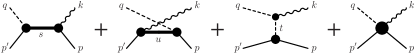
Figure 1: Generic structure of the pion photoproduction current $M^{\mu}$ for $\gamma N\to\pi N$ according to Eq. (1). Time proceeds from right to left. Nucleons and pions are depicted by solid and dashed lines, respectively, and the photon is shown as a wavy line. The four-momenta shown at the external lines are those of the respective particles used in this work. The first three diagrams comprising class-A diagrams GellMann54 depict the $s$-, $u$-, and $t$-channel pole diagrams $M^{\mu}_{s}$, $M^{\mu}_{u}$, and $M^{\mu}_{t}$, respectively, where $s$, $u$, and $t$ are the respective Mandelstam variables of the internally exchanged particles, as indicated. The last diagram (called class B GellMann54 ) shows the contact-type interaction current $M^{\mu}_{\text{int}}$.

One can easily show that assuming the validity of the usual WTI (3) for the electromagnetic nucleon current $J^{\mu}$ and its analog for the pion current, the generalized WTI (2) implies

$$k_{\mu}\,M^{\mu}_{\text{int}}=-\tilde{F}_{s}e_{i}+\tilde{F}_{u}e_{f}+\tilde{F}_{t}e_{\pi}\leavevmode\nobreak\ ,$$ (4)

where the $\tilde{F}_{x}$ are the vertices $F_{x}$ of (2) stripped of their isospin operators $\tau$ that now appear in

$$e_{i}=\tau Q_{i}\leavevmode\nobreak\ ,\qquad e_{f}=Q_{f}\tau\leavevmode\nobreak\ ,\quad\text{and}\quad e_{\pi}=Q_{\pi}\tau$$ (5)

which are the charges for all external hadron legs in an appropriate isospin basis (with all corresponding indices and summations suppressed). In other words, the relation

$$e_{i}=e_{f}+e_{\pi}$$ (6)

describes charge conservation for the pion photoproduction process. With the single-particle WTIs for nucleons and pions given, Eq. (4) is completely equivalent to the generalized WTI (2). It is this Eq. (4) for the contact-type interaction current $M^{\mu}_{\text{int}}$, in particular, that is being exploited here for the purposes of preserving the overall gauge invariance of the production current.

II.1 Dyson-Schwinger framework

The complete (i.e., fully dressed, non-linear, and gauge-invariant) structure of pion photoproduction was described by Haberzettl Haberzettl97 within a covariant field-theoretical Dyson-Schwinger framework. In practice, however, the complexity of the full formalism needs to be truncated at some level to make it numerically tractable. Since doing so invariably leads to a violation of gauge invariance, one must find prescriptions to restore this fundamental symmetry. And one should do so in a manner that incorporates as many of the original reaction mechanisms as possible. Particularly relevant in this context are the hadronic final-state interactions of the outgoing meson-nucleon states since these form essential parts of the dynamical content of the interaction current $M^{\mu}_{\text{int}}$ Haberzettl97 .

In Ref. Haberzettl06 , it was shown how to approximate the full formalism in a manner that includes the full hadronic final-state interactions while at the same time preserving the gauge invariance by reproducing the generalized Ward-Takahashi identity (2) for the production current. In the present paper, we will follow the variant of the procedure of Ref. Haberzettl06 put forward recently in Ref. HHN2011 . We emphasize that without any approximation, i.e., as full Dyson-Schwinger formulations, the respective results of Refs. Haberzettl06 ; Haberzettl97 ; HHN2011 are completely equivalent. However, the features of Ref. HHN2011 turn out to be particularly well suited for approximating the dressing effects of the electromagnetic nucleon current $J^{\mu}$ in a way that is reciprocally consistent with the production current $M^{\mu}$ itself while at the same time preserving local gauge invariance. Here, we will recapitulate the details of the approach given in Ref. HHN2011 only insofar as it is necessary for the present application. To this end, we make extensive use of diagrammatic representations. Full details and derivations can be found in Ref. HHN2011 , and in Refs. Haberzettl97 ; Haberzettl06 .

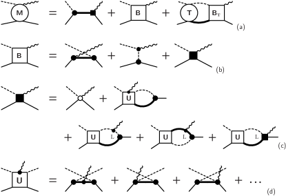
Figure 2: Microscopic structure of the photoproduction process according to Ref. HHN2011 . The line styles are the same as in Fig. 1, with thick solid nucleon lines depicting the propagation of dressed intermediate nucleons. Solid and open circles indicate dressed and bare vertices, respectively. (a) The full current $M^{\mu}$ with its FSI contribution written as a loop integration over the full $\pi N$ $T$-matrix. (b) Details of the Born-type current $B^{\mu}$ of Eq. (8) that comprises the $u$ and $t$-channel contributions $M^{\mu}_{u}$ and $M^{\mu}_{t}$, and the contact-type four-point current $M^{\mu}_{c}$ depicted as a solid square whose details in turn are shown in part (c). The first term here is the Kroll-Ruderman contact term $m^{\mu}_{\textsc{kr}}$. The various hadronic boxes labeled $U$ depict the non-polar $\pi N$ irreducible driving term of the $\pi N$ $T$-matrix, as shown in Fig. 4(c). The particular five-point current $U^{\mu}$ appearing in the first loop arises from attaching a photon to $U$; its lowest order is shown in part (d). The four-point currents appearing here correspond to the full interaction current $M^{\mu}_{\text{int}}$ of Fig. 1. The box labeled $B_{\textsc{t}}$ in (a) and the loop integrations labeled L in (c) indicate restrictions of the corresponding $B^{\mu}$ contributions to transverse and longitudinal pieces, respectively (see text). The details of the full nucleon current $J^{\mu}$ (solid circle) and its auxiliary $s$-channel restriction $\tilde{J}^{\mu}_{s}$ (solid square) are depicted in Fig. 3.

Note that on the hadronic side, for simplicity, we will speak here most of the time explicitly only of pions and nucleons. However, these particles are to be taken as representatives for all mesons and baryons, respectively, that take part in a particular application. Correspondingly, any explicit equation appearing here for the $\pi N$ channel is to be read as a matrix equation that couples all hadronic meson-baryon channels once the full complexity of the reaction dynamics is turned on.

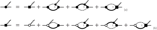
Figure 3: (a) The dressed electromagnetic nucleon current $J^{\mu}$, with the first term on the right-hand side (depicted as a solid-square three-point current) corresponding to $\tilde{J}^{\mu}_{s}$ appearing in Eq. 7. (b) The details of $\tilde{J}^{\mu}_{s}$. The first term (with open circle) is the bare current and the second term contains the Kroll-Ruderman term (open-circle four-point current) integrated over by the dressed $\pi NN$ vertex (solid circle; cf. Fig. 5). The remaining loop contributions only contribute longitudinally (as indicated by the index L). By contrast, the loops in (a) only contribute transversally, as indicated by the letter T. The solid-square contact-type four-point current $M^{\mu}_{c}$ in the loops at the end of both lines is given in Fig. 2(c).

Following Ref. HHN2011 , the full pion photoproduction current $M^{\mu}$ in the one-photon approximation can be written as

$$M^{\mu}=F_{s}S\tilde{J}^{\mu}_{s}+B^{\mu}+TG_{0}B^{\mu}_{\textsc{t}}\leavevmode\nobreak\ ,$$ (7)

with the non-pole Born-type current given by

$$B^{\mu}=M^{\mu}_{u}+M^{\mu}_{t}+M^{\mu}_{c}\leavevmode\nobreak\ .$$ (8)

These equations are depicted diagrammatically in Fig. 2. The (fully dressed) $u$- and $t$-channel contributions $M^{\mu}_{u}$ and $M^{\mu}_{t}$ of Eq. (1) appear here unchanged, but the $s$-channel current $M^{\mu}_{s}$ and the interaction current $M^{\mu}_{\text{int}}$ are now spread out over the remaining terms. The first term, $F_{s}S\tilde{J}^{\mu}_{s}$, contains part of the $s$-channel pole contribution via the fully dressed nucleon propagator $S$, however, with an electromagnetic current contribution $\tilde{J}^{\mu}_{s}$ for the nucleon that is only part of the full nucleon current $J^{\mu}$. The situation is depicted in Fig. 3 and will be discussed in more detail below. The contact term $M^{\mu}_{c}$ [see Fig. 2(c)] contains part of the full interaction current $M^{\mu}_{\text{int}}$. The remaining pieces for both $M^{\mu}_{s}$ and $M^{\mu}_{\text{int}}$ come from the $TG_{0}B^{\mu}_{\textsc{t}}$ term which describes the $\pi N$ final-state interaction mediated by the loop integration over the full $\pi N$ $T$-matrix, where $G_{0}$ is the intermediate propagator of the free $\pi N$ pair within the loop. Note that only the transverse parts of the contributions of these loop integrations are to be taken into account here, as indicated by the index T. The respective missing pieces for $M^{\mu}_{s}$ and $M^{\mu}_{\text{int}}$ arise from splitting the full $T$ into an $s$-channel pole part and a non-pole part according to

$$T=\ket{F}S\bra{F}+X\leavevmode\nobreak\ ,$$ (9)

where the first term contains the $s$-channel nucleon pole via the dressed nucleon propagator $S$ and $X$ denotes the remaining non-pole part. This splitting is depicted diagrammatically in Fig. 4 together with the Bethe-Salpeter equation for the non-pole amplitude,

$$X=U+UG_{0}X\leavevmode\nobreak\ ,$$ (10)

driven by the (fully dressed) non-pole $\pi N$ irreducible mechanisms subsumed in $U$ whose lowest-order contribution is the $u$-channel exchange shown in Fig. 4(c). The $F$’s here are the fully dressed $\pi NN$ vertices related to the bare vertex $f$ by

$$\ket{F}=\ket{f}+XG_{0}\ket{f}\leavevmode\nobreak\ .$$ (11)

This dressed vertex is represented diagrammatically in Fig. 5 together with the dressing mechanism for the nucleon propagator

$$S=S_{0}+S_{0}\Sigma S$$ (12)

given in terms of the bare propagator $S_{0}$ and the nucleon self-energy loop $\Sigma$.

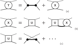
Figure 4: (a) Representing the full $T$-matrix for $\pi N$ scattering via its (fully dressed) $s$-channel pole part and its non-polar contribution $X$, according to Eq. (9). (b) The Bethe-Salpeter scattering equation for the non-pole amplitude $X$, Eq. (10). Its driving term $U$ comprises all $\pi N$ irreducible mechanisms. The corresponding lowest-order contribution is the $u$-channel exchange shown explicitly in (c). Attaching a photon to this diagram provides the five-point current given in Fig. 2(d).

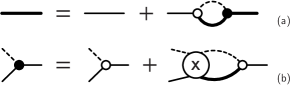
Figure 5: Dressing mechanisms for (a) the nucleon propagator $S$ in terms of the bare propagator $S_{0}$ (thin line) and the self-energy loop and (b) the $\pi NN$ vertex $F$ according to Eq. (11). Dressed and undressed vertices are shown as solid and open circles, respectively.

The entire set of equations summarized by Figs. 2 through 5 provides a complete solution of the problem by forming a tower of coupled non-linear Dyson-Schwinger-type equations that can only be solved iteratively. Viewing this coupled set in its entirety for a given bare input, the splitting (9) of $T$ into pole and non-pole contributions is unique. However, this uniqueness generally is lost once approximations are introduced. As a consequence, the resulting individual pieces of a particular approximation of the splitting (9) may exhibit undesirable numerical artifacts which the $T$ matrix itself does not possess. (This is the case, for example, for pole and non-pole parts resulting from the Jülich model we use here Doring09L .) In order to avoid such problems to some extent, one may, instead of Eq. (10), employ the Bethe-Salpeter equation

$$T=V+VG_{0}T$$ (13)

for the entire $T$-matrix, with the driving term

$$V=\ket{f}S_{0}\bra{f}+U\leavevmode\nobreak\ ,$$ (14)

where $f$ and $S_{0}$ are the bare vertex and bare propagator of Eqs. (11) and (12), respectively.

The photoproduction current of Eq. (7) is formulated assuming that the hadronic scattering information enters the problem in terms of $T$, i.e., in terms of a matrix coupled-channels equation of the generic type given in (13). An equivalent formulation in terms of $X$ exists Haberzettl97 ; HHN2011 , however, since the usual hadronic coupled-channels approaches (like the Jülich model we employ here) produce full $T$-matrices as a matter of course, it is of considerable practical advantage to utilize this information directly for the photoproduction current. (See also the corresponding discussion at the end of Sec. III.)

II.2 Gauge-invariant truncation of the pion photoproduction current

As mentioned, the preceding formulation is exact, but it is also very complex in detail and therefore, at present at least, cannot be solved in its entirety without making some approximations to render the problem manageable numerically. In the particular formulation HHN2011 used here, there are two obvious places for such approximations — the dressed nucleon current $J^{\mu}$ depicted in Fig. 3 and the contact-type five-point current $M^{\mu}_{c}$ shown in Fig. 2(c).

The detailed (exact) structure of the electromagnetic nucleon $J^{\mu}$ is given by HHN2011

$$J^{\mu}=\tilde{J}^{\mu}_{s}+\bra{F}G_{0}\left(M^{\mu}_{u}+M^{\mu}_{t}+M^{\mu}_{c}\right)_{\textsc{t}}\leavevmode\nobreak\ ,$$ (15)

as one easily reads off Fig. 3. The currents within the loop structure here are given entirely by pieces occurring in the pion production current itself. As was shown in Ref. HHN2011 , this reciprocal consistency between the nucleon current $J^{\mu}$ and the production current $M^{\mu}$ was essential for deriving the particular form of $M^{\mu}$ given in Eq. (7) because the transverse loop contributions of Eq. (15), in particular, survive unchanged in the loop integration that provides the FSI contribution in Eq. (7). This form, moreover, easily permits to treat both $J^{\mu}$ and $M^{\mu}$ with a consistent set of approximations.

II.2.1 Approximating the nucleon current $J^{\mu}$

First, we note that all loop integrations in Eqs. (7) and (15) contain the full nucleon current within the $u$-channel loops. The nucleon current, thus, couples back into itself and these contributions, therefore, are part of the non-linear hierarchy of Dyson-Schwinger equations that, in principle, needs to be solved iteratively requiring prohibitive amounts of computational resources. To avoid this complication, we truncate these loop contributions by employing in our present application only the usual (on-shell) $\gamma^{\mu}$ and $\sigma^{\mu\nu}k_{\nu}$ pieces for the nucleon current within all the loops. This approximation step thus linearizes the nucleon-current contributions. Second, we note that the current piece $\tilde{J}^{\mu}_{s}$ that appears in the $s$-channel part of (7) obeys the same WTI (3) as the full current, i.e.,

$$k_{\mu}J^{\mu}=k_{\mu}\tilde{J}^{\mu}_{s}=S^{-1}(p+k)Q_{N}-Q_{N}S^{-1}(p)\leavevmode\nobreak\ ,$$ (16)

since the their difference in (15) is purely transverse. The detailed expressions for $\tilde{J}^{\mu}_{s}$, moreover, mainly are comprised of longitudinal contributions that arise from the photon being attached to the self-energy loop of the nucleon propagator [cf. Figs. 3(b) and 5(a)].

To reproduce the WTI (16), it is convenient to utilize the Ball-Chiu current BallChiu1980 ,

$$J^{\mu}_{s} =(2p+k)^{\mu}\frac{S^{-1}(p+k)Q_{N}-Q_{N}S^{-1}(p)}{s^{2}-p^{2}}$$

$$\mbox{}\quad+\left[\gamma^{\mu}-\frac{(2p+k)^{\mu}}{s-p^{2}}k\!\!\!/\right]Q_{N}\frac{A(s)+A(p^{2})}{2}\leavevmode\nobreak\ ,$$ (17)

where $s=(p+k)^{2}$ and $A$ is one of two scalar dressing functions ($B$ being the other) resulting from the generic form

$$S(p)=\frac{1}{p\!\!\!/A(p^{2})-mB(p^{2})}$$ (18)

of the dressed nucleon propagator; $m$ is the nucleon mass. The dressing functions $A(p^{2})$ and $B(p^{2})$ are constrained to produce a unit residue at the nucleon pole where $p^{2}=m^{2}$ Haberzettl97 ; AA95 . By construction, $J^{\mu}_{s}$ is the minimal current that satisfies the WTI (16) for fully dressed propagators and it is both non-singular and symmetric. Without lack of generality, therefore, we may write

$$\tilde{J}_{s}^{\mu}=J^{\mu}_{s}+\tilde{T}^{\mu}_{s}\leavevmode\nobreak\ ,$$ (19)

where $\tilde{T}^{\mu}$ is the transverse remainder defined by this relation.

Within the $s$-channel context of Eq. (7), the Ball-Chiu current provides a particularly simple expression when considering the half-on-shell situation, with an incoming nucleon spinor $u(p)$ on the right and an outgoing propagator $S(p+k)$ on the left. One easily finds

$$SJ^{\mu}_{s}u =\Bigg{[}\frac{1}{p\!\!\!/+k\!\!\!/-m}\left(\gamma^{\mu}+\frac{i\sigma^{\mu\nu}k_{\nu}}{2m}\kappa_{1}\right)$$

$$\qquad\mbox{}+i\sigma^{\mu\nu}k_{\nu}\frac{\kappa_{2}-\kappa_{1}}{s-m^{2}}\Bigg{]}Q_{N}\,u(p)\leavevmode\nobreak\ ,$$ (20)

where $p^{2}=m^{2}$. Albeit written in a somewhat different way, this expression is equivalent to Eq. (17) of Ref. HHN2011 , and the two independent coefficient functions $\kappa_{i}=\kappa_{i}(s)$ ($i=1,2$) that are directly related to the propagator dressing functions $A$ and $B$ are given in Eq. (19) of Ref. HHN2011 . We omit their details because we will not make use of them here. We only mention that the on-shell values at $s=m^{2}$ for both coefficients are identical, i.e., $\kappa_{1}(m^{2})=\kappa_{2}(m^{2})=A(m^{2})-1$, and that one easily finds that $(\kappa_{2}-\kappa_{1})/(s-m^{2})$ possesses a finite limit for $s\to m^{2}$ if we assume that the dressing functions $A$ and $B$ are analytic functions in the vicinity of $s=m^{2}$. This means they both vanish in the structureless limit [where $A(m^{2})=1$], thus leaving in (20) only the usual $\gamma^{\mu}$ Dirac current together with a structureless propagator. All effects of the dressing thus reside in the terms that depend on the $\kappa_{i}$ whose overall contributions are manifestly transverse. In the present application, we will absorb the $\kappa_{i}$ ($i=1,2$) dependence in some fit parameters.

We note in this context that the Ball-Chiu current $J^{\mu}_{s}$ does not fully contain the anomalous-moment contribution of the usual Pauli part of the on-shell nucleon current. These anomalous contributions arise from other transverse dressing mechanisms. Writing the on-shell matrix element of the full nucleon current between nucleon spinors in the usual manner as

$$\bar{u}J^{\mu}u=e\bar{u}\left(\gamma^{\mu}\delta_{N}+\frac{i\sigma^{\mu\nu}k_{\nu}}{2m}\kappa_{N}\right)u\leavevmode\nobreak\ ,$$ (21)

where $e$ is the fundamental charge unit, $\kappa_{N}$ is the anomalous moment of the nucleon, and $\delta_{N}=1,0$ for the proton and neutron, respectively, the anomalous part can be written as

$$e\,\bar{u}\left(\frac{i\sigma^{\mu\nu}k_{\nu}}{2m}\kappa_{N}\right)u =\bar{u}\Bigg{(}e\delta_{N}\frac{i\sigma^{\mu\nu}k_{\nu}}{2m}\tilde{\kappa}_{0}$$

$$\qquad\mbox{}+\tilde{T}^{\mu}+\bra{F}G_{0}B^{\mu}_{\textsc{t}}\Bigg{)}u\leavevmode\nobreak\ ,$$ (22)

where $\tilde{\kappa}_{0}=\kappa_{1}(m^{2})=\kappa_{2}(m^{2})=A(m^{2})-1$. This result follows from Eq. (15) utilizing Eq. (19) and the expression (20) performing expansions of $\kappa_{i}(s)$ around $s=m^{2}$. In principle, this equation is exact if $\tilde{T}^{\mu}$ and $B^{\mu}_{\textsc{t}}$ could be calculated without approximations. We see here that for the proton, the Ball-Chiu term $\tilde{\kappa}_{0}$ contributes partially to the anomalous moment, but for the neutron, it does not contribute at all.

In Ref. HHN2011 , it was advocated to put $\tilde{T}^{\mu}=0$ and ensure the anomalous contributions by adding a contact term to the approximation of $M^{\mu}_{c}$ to be discussed in the following subsection in the context of Eq. (30). In the present application, however, we proceed differently. We expand the full dressing functions $\kappa_{i}$ appearing in the Ball-Chiu contribution (20) around their on-shell points and use the resulting coefficients as fit parameters. In addition, we assume that we can approximate $\tilde{T}^{\mu}$ by a single transverse contact term whose operator structure is given by $\sigma^{\mu\nu}k_{\nu}$ alone. It is the corresponding coefficient, in particular, that ensures that we can reproduce the anomalous moments. For the half-on-shell matrix element of $\tilde{J}_{s}^{\mu}$ appearing in the $s$-channel pole term of Eq. (7), we then obtain the approximation

$$S\tilde{J}^{\mu}_{s}u\to S\tilde{J}^{\mu}_{s}u =e\Bigg{[}\frac{1}{p\!\!\!/+k\!\!\!/-m}\left(\delta_{N}\gamma^{\mu}+\frac{i\sigma^{\mu\nu}k_{\nu}}{2m}\kappa_{0}\right)$$

$$\qquad\mbox{}+\frac{t^{\mu\nu}k_{\nu}}{4m^{2}}C_{1}+\frac{i\sigma^{\mu\nu}k_{\nu}}{4m^{2}}C_{2}\Bigg{]}u(p)\leavevmode\nobreak\ ,$$ (23)

where

$$t^{\mu\nu}k_{\nu}=\frac{\gamma^{\mu}(s-m^{2})-(2p+k)^{\mu}k\!\!\!/}{2m}$$ (24)

is a transverse current operator that follows from the expansions of the Ball-Chiu contributions. For each nucleon, this approximation contains three dimensionless coefficients: a real parameter $\kappa_{0}$, and two complex numbers $C_{1}$ and $C_{2}$ for the contact contributions.

We emphasize that the approximation just discussed only pertains to the true nucleon current. In the full coupled-channels treatment, the structure of Eq. (7) also comprises contributions from currents $\tilde{J}^{\mu}_{s}$ that describe nucleon-resonance transitions. Such transition currents, however, must necessarily be transverse and thus correspond only to the first two diagrams on the right-hand side of Fig. 3(b). In the present applications, thus, we describe these transition currents by the point vertices of the nucleon-resonance photo-transition Lagrangians given in Eqs. (52) and (53) of the Appendix.

We also emphasize that the present approximate treatment of the $s$-channel term (23) that permits one to describe the corresponding fully dressed contribution in terms of three parameters requires the complete reciprocal consistency between the nucleon current and the photoproduction current, as derived in Ref. HHN2011 . The approximation scheme of Ref. Haberzettl06 , by contrast, is ambiguous in its treatment of certain transverse current contributions that have no bearing on gauge invariance. Specifically, the undetermined transverse current $T^{\mu}$ appearing in Eq. (21) of Ref. Haberzettl06 was taken to be zero in the preliminary applications reported there. To achieve complete structural equivalence with the present results, one finds that $T^{\mu}$ must be chosen as $T^{\mu}=UG_{0}(M^{\mu}_{c})_{\textsc{t}}$ instead if one wants to preserve the equivalence even when making approximations.

II.2.2 Approximating the four-point contact current $M^{\mu}_{c}$

In view of the fact that the FSI loop in (7) is transverse and that the approximation of the $s$-channel current $\tilde{J}^{\mu}_{s}$ by the Ball-Chiu current $J^{\mu}_{s}$ leaves the corresponding WTI unchanged, the entire burden for reproducing the generalized WTI for the production current $M^{\mu}$ rests with the contact-type four point current $M^{\mu}_{c}$ whose four-divergence, by construction, must be the same as that of the interaction current $M^{\mu}_{\text{int}}$ in Eq. (4), i.e.,

$$k_{\mu}\,M^{\mu}_{\text{int}}=k_{\mu}M^{\mu}_{c}=-\tilde{F}_{s}e_{i}+\tilde{F}_{u}e_{f}+\tilde{F}_{t}e_{\pi}\leavevmode\nobreak\ .$$ (25)

As far as preserving gauge invariance is concerned, therefore, the situation is very much the same as in the approach of Ref. Haberzettl06 , even though the details of the present formulation are somewhat different. In other words, any approximation of $M^{\mu}_{c}$ must satisfy the constraint (25).

The internal dynamical mechanisms of $M^{\mu}_{c}$ as depicted in Fig. 2(c) are quite involved and cannot, at present, be incorporated fully in numerical applications. In Ref. Haberzettl06 , it was discussed in detail how to find approximations of the mechanisms within $M^{\mu}_{c}$ at any desired level of sophistication while still reproducing (25). For the present application, we simply quote the results of Haberzettl06 valid when the $\pi NN$ vertices are described by phenomenological form factors, as it is the case here.

Phenomenologically, the $\pi NN$ vertex stripped of its isospin dependence can be written as

$$\tilde{F}_{x}=g_{\textit{NN}\pi}\frac{\gamma_{5}q\!\!\!/}{2m}f_{x}\leavevmode\nobreak\ ,$$ (26)

where we take here pure pseudovector coupling, with $g_{\textit{NN}\pi}$ being the physical coupling constant. The subscript $x=s$, $u$, or $t$ indicates the kinematic context; $f_{x}$ is the phenomenological form factor for the corresponding reaction channel normalized to unity when all hadron legs are on-shell and $q$ is the four-momentum of the outgoing meson. Following Ref. Haberzettl06 , we define an auxiliary current

$$C^{\mu} =-\,e_{\pi}\frac{f_{t}-\hat{F}}{t-q^{2}}(2q-k)^{\mu}-e_{f}\frac{f_{u}-\hat{F}}{u-p^{\prime 2}}(2p^{\prime}-k)^{\mu}$$

$$\qquad\mbox{}-\,e_{i}\frac{f_{s}-\hat{F}}{s-p^{2}}(2p+k)^{\mu}\leavevmode\nobreak\ ,$$ (27)

with

$$\hat{F}=1-\hat{h}\left(1-\delta_{s}f_{s}\right)\left(1-\delta_{u}f_{u}\right)\left(1-\delta_{t}f_{t}\right)\leavevmode\nobreak\ ,$$ (28)

where the four-momenta are those given in Fig. 1. The constant $\delta_{x}$ is unity if the corresponding $x$-channel contributes to the reaction in question, and zero otherwise. The parameter $\hat{h}$ may be an arbitrary (complex) function, $\hat{h}=\hat{h}(s,u,t)$, possibly subject to crossing-symmetry constraints. In the present work, it is simply taken as a fit constant for the sake of simplicity. The four-divergence of the auxiliary current evaluates to

$$k_{\mu}C^{\mu}=-f_{s}e_{i}+f_{u}e_{f}+f_{t}e_{\pi}\leavevmode\nobreak\ .$$ (29)

We emphasize that $C^{\mu}$ is non-singular since, by construction, the propagator singularities are canceled by the corresponding zeros of $f_{x}-\hat{F}$. In other words, $C^{\mu}$ is a true contact current.

The gauge-invariance preserving (GIP) approximation of the contact current $M^{\mu}_{c}$ then may be chosen as Haberzettl06 ; HHN2011

$$M^{\mu}_{c}\to M^{\mu}_{c} =g_{\textit{NN}\pi}\frac{\gamma_{5}(q\!\!\!/-\beta k\!\!\!/)}{2m}\,C^{\mu}$$

$$\mbox{}\qquad-g_{\textit{NN}\pi}\frac{\gamma_{5}\gamma^{\mu}}{2m}\left(e_{\pi}f_{t}-\beta k_{\rho}C^{\rho}\right)\leavevmode\nobreak\ ,$$ (30)

where $\beta$ is a free fit parameter. One can easily check that this choice for $M^{\mu}_{c}$ satisfies the gauge-invariance condition (25). Essential in this respect is the relation (29). Note that the term proportional to the pion charge $e_{\pi}$ in (30) is a dressed version of the familiar Kroll-Ruderman contact current where the dressing form factor $f_{t}$ is that of the $t$-channel amplitude $M^{\mu}_{t}$. The original (undressed) Kroll-Ruderman term survives in this GIP current since $f_{t}=1+(f_{t}-1)$, i.e., the dressing is given by the additional $f_{t}-1$ contribution.

We emphasize that the present formulation is equally valid for real and virtual photons. For pion photoproduction with real photons, in particular, only transverse currents contribute to the physical amplitude. The longitudinal loop contributions shown for $M^{\mu}_{c}$ in Fig. 2(c), therefore, are projected out and only the (bare) Kroll-Ruderman current and the loop over the the five-point interaction current $U^{\mu}$ of Fig. 2(d) remain. Hence, subtracting the usual (bare) Kroll-Ruderman term from the GIP current (30), the remaining expression is a phenomenological approximation of the latter loop contribution for real photons.

Finally, we mention that when we consider intermediate channels other than $\pi N$ (cf. Sec. IV below), the corresponding contact currents $M^{\mu}_{c}$ that appear in the transverse loops $TG_{0}B^{\mu}_{\textsc{t}}$ of Eq. (7) are easily constructed in analogy to the explicit $\pi N$ case given here by using the generic constraint (25).

II.2.3 Covariant three-dimensional reduction

The present formalism is a fully covariant approach. To calculate any reaction amplitude in a full four-dimensional framework is a daunting numerical task. Therefore, in the present work, we approximate the full meson-baryon two-body propagator $G_{0}$ by the Kadyshevsky propagator BbS , as specified in Eqs. (36) and (37) in the next section. This propagator, together with an implied energy delta function, restricts the propagation of the intermediate meson and baryon to their respective energy shells, thus reducing the four-dimensional loop integration to a three-dimensional one without destroying the covariance of the equation. This reduction is also necessary to be able to match up the hadronic Jülich-model input with the present formalism.

III Making the Jülich $\pi N$ model compatible with the present approach

In the present work, we employ the Jülich dynamical coupled-channels $\pi N$ model Schutz98 ; Krehl00 ; Gasparyan03 to account for the hadron dynamics. As mentioned in the Introduction, this model is formulated within time-ordered perturbation theory (TOPT) which is a non-covariant three-dimensional formalism Schweber . We, therefore, need to provide a procedure to match it to the covariance of the present photoproduction formalism.

To this end, we first note that the Jülich $T$-matrix satisfies the three-dimensional Lippmann-Schwinger-type equation

$$T_{{\text{TO}}}(\textbf{p}^{\prime},\textbf{p};z) =V_{{\text{TO}}}(\textbf{p}^{\prime},\textbf{p};z)$$

$$\mbox{}+\int d^{3}p^{\prime\prime}\,V_{{\text{TO}}}(\textbf{p}^{\prime},\textbf{p}^{\prime\prime};z)\,G_{{\text{TO}}}(\textbf{p}^{\prime\prime},z)T_{{\text{TO}}}(\textbf{p}^{\prime\prime},\textbf{p};z)\leavevmode\nobreak\ ,$$ (31)

where $z$ denotes the total-energy variable and TO indicates that all entities result from the time-ordered formalism. The intermediate pion-nucleon propagator reads

$$G_{{\text{TO}}}(\textbf{p}^{\prime\prime},z)=\frac{1}{z-E(\textbf{p}^{\prime\prime})-\omega(\textbf{p}^{\prime\prime})+i0}\leavevmode\nobreak\ ,$$ (32)

where $E(\textbf{p}^{\prime\prime})\equiv\sqrt{m^{2}+\textbf{p}^{\prime\prime 2}}$ stands for the energy of the nucleon and $\omega(\textbf{p}^{\prime\prime})\equiv\sqrt{m_{\pi}^{2}+\textbf{p}^{\prime\prime 2}}$ for the energy of the pion, with the mass $m_{\pi}$. The complex notation $i0$ indicates the physical limit to the upper edge of the scattering cut to provide proper boundary conditions. Equation (31) written in the c.m. system is structurally very similar to the Bethe-Salpeter equation (13) after it has been subjected to a covariant three-dimensional reduction. Therefore, to match the two, one needs to ensure that Eq. (31) transforms covariantly away from the c.m. system.

Table 1: Cutoff parameters (in MeV) in the form factors of Eqs. (54) and (55).

$\Lambda$	$\Lambda_{B}$	$\Lambda_{\pi}$	$\Lambda_{v}$
$600$	$725$	$1343$	$1645$

Table 2: Effective electromagnetic coupling constants for isospin $1/2$ resonances. The subscripts $p$ and $n$ denote the resonance coupling to $\gamma p$ and $\gamma n$, respectively.

	$D_{13}(1520)$	$S_{11}(1535)$	$S_{11}(1650)$	$P_{13}(1720)$
$\leavevmode\nobreak\ \leavevmode\nobreak\ g_{p}^{(1)}$	$-1.23\leavevmode\nobreak\ \leavevmode\nobreak\ \leavevmode\nobreak\$	$-1.14\leavevmode\nobreak\ \leavevmode\nobreak\ \leavevmode\nobreak\$	$0.02\leavevmode\nobreak\ \leavevmode\nobreak\ \leavevmode\nobreak\$	$4.23\leavevmode\nobreak\ \leavevmode\nobreak\ \leavevmode\nobreak\$
$\leavevmode\nobreak\ \leavevmode\nobreak\ g_{p}^{(2)}$	$1.58\leavevmode\nobreak\ \leavevmode\nobreak\ \leavevmode\nobreak\$			$-12.56\leavevmode\nobreak\ \leavevmode\nobreak\ \leavevmode\nobreak\$
$\leavevmode\nobreak\ \leavevmode\nobreak\ g_{n}^{(1)}$	$2.69\leavevmode\nobreak\ \leavevmode\nobreak\ \leavevmode\nobreak\$	$0.21\leavevmode\nobreak\ \leavevmode\nobreak\ \leavevmode\nobreak\$	$-0.17\leavevmode\nobreak\ \leavevmode\nobreak\ \leavevmode\nobreak\$	$-0.73\leavevmode\nobreak\ \leavevmode\nobreak\ \leavevmode\nobreak\$
$\leavevmode\nobreak\ \leavevmode\nobreak\ g_{n}^{(2)}$	$-3.58\leavevmode\nobreak\ \leavevmode\nobreak\ \leavevmode\nobreak\$			$2.52\leavevmode\nobreak\ \leavevmode\nobreak\ \leavevmode\nobreak\$

Table 3: Effective electromagnetic coupling constants for isospin $3/2$ resonances.

	$P_{33}(1232)$	$S_{31}(1620)$	$D_{33}(1700)$	$P_{31}(1910)$
$\leavevmode\nobreak\ \leavevmode\nobreak\ g^{(1)}$	$2.01\leavevmode\nobreak\ \leavevmode\nobreak\ \leavevmode\nobreak\$	$1.63\leavevmode\nobreak\ \leavevmode\nobreak\ \leavevmode\nobreak\$	$-6.56\leavevmode\nobreak\ \leavevmode\nobreak\ \leavevmode\nobreak\$	$-1.44\leavevmode\nobreak\ \leavevmode\nobreak\ \leavevmode\nobreak\$
$\leavevmode\nobreak\ \leavevmode\nobreak\ g^{(2)}$	$4.48\leavevmode\nobreak\ \leavevmode\nobreak\ \leavevmode\nobreak\$		$5.38\leavevmode\nobreak\ \leavevmode\nobreak\ \leavevmode\nobreak\$

We define now

$$V(\textbf{p}^{\prime},\textbf{p};\sqrt{s}) \equiv(2\pi)^{3}\rho(\textbf{p}^{\prime})\,V_{{\text{TO}}}(\textbf{p}^{\prime},\textbf{p};z)\,\rho(\textbf{p})\leavevmode\nobreak\ ,$$ (33)

$$T(\textbf{p}^{\prime},\textbf{p};\sqrt{s}) \equiv(2\pi)^{3}\rho(\textbf{p}^{\prime})\,T_{{\text{TO}}}(\textbf{p}^{\prime},\textbf{p};z)\,\rho(\textbf{p})\leavevmode\nobreak\ ,$$ (34)

where

$$\rho(\textbf{p})=2\sqrt{E(\textbf{p})\omega(\textbf{p})}$$ (35)

corrects the non-covariant normalizations of the TOPT plane-wave states and where the invariant mass $\sqrt{s}$ is defined as $\sqrt{s}\equiv z$ in the c.m. system. Equation (31) then may be recast in the equivalent form

$$T(\textbf{p}^{\prime},\textbf{p};\sqrt{s}) =V(\textbf{p}^{\prime},\textbf{p};\sqrt{s})$$

$$\mbox{}+\int\frac{d^{3}p^{\prime\prime}}{(2\pi)^{3}}\,V(\textbf{p}^{\prime},\textbf{p}^{\prime\prime};\sqrt{s})\,G_{0}(\textbf{p}^{\prime\prime},\sqrt{s})\,T(\textbf{p}^{\prime\prime},\textbf{p};\sqrt{s})\leavevmode\nobreak\ ,$$ (36)

where

$$G_{0}(\textbf{p}^{\prime\prime},\sqrt{s})\equiv\frac{1}{\rho^{2}(\textbf{p}^{\prime\prime})}\;\frac{1}{\sqrt{s}-E(\textbf{p}^{\prime\prime})-\omega(\textbf{p}^{\prime\prime})+i0}\leavevmode\nobreak\ .$$ (37)

Equation (36) is formally identical to the Kadyshevsky equation BbS which is the result of a particular covariant three-dimensional reduction of the Bethe-Salpeter equation that preserves elastic unitarity. Hence, utilizing the time-ordered Jülich $T$-matrix in the redefined form (34) is completely consistent with the covariant three-dimensional reduction of the photoproduction current given in Eq. (7). For the corresponding reduced meson-baryon propagator one must use the form (37), of course.

Table 4: Dimensionless parameters $C_{1}$, $C_{2}$, and $\kappa_{0}$ in the electromagnetic nucleon current, Eq. (23).

	$C_{1}$	$C_{2}$	$\kappa_{0}$
proton	$2.07\,{e}^{-1.74i}$	$34.62\,{e}^{0.09i}$	$-4.24\leavevmode\nobreak\ \leavevmode\nobreak\$
neutron	$12.35\,{e}^{2.52i}$	$25.96\,{e}^{2.79i}$	$3.24$

Table 5: Dimensionless parameters $\hat{h}$ and $\beta$ in the contact current $M^{\mu}_{c}$, Eq. (30), for the various meson-baryon channels.

	$\pi^{+}n$	$\pi^{0}p\leavevmode\nobreak\$	$\pi^{-}p$	$\eta p\leavevmode\nobreak\$	$\pi\Delta\leavevmode\nobreak\$
$\leavevmode\nobreak\ \leavevmode\nobreak\ \hat{h}$	$1.43$	$1.44$	$2.01$	$-10.04$	$0.74$
$\leavevmode\nobreak\ \leavevmode\nobreak\ \beta$	$-0.17$	$-1.43$	$-0.10$	$3.45$	$-1.75$

We recall in this context that pions and nucleons are used here as simplified generic tags for all mesons and baryons incorporated in the Jülich model. Therefore, all entities discussed here need to be considered as elements of matrices labeled by meson-baryon channels and all equations contain implied summations over all elements of this channel space. Moreover, for quasi-two-body channels $\sigma N$, $\rho N$, and $\pi\Delta$, the propagator (37) is to be slightly modified by including the self-energy of the corresponding quasi-free particles Schutz98 ; Krehl00 .

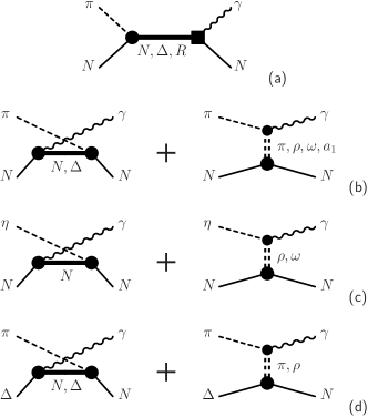
Figure 6: Hadronic states taken into account in the present model (see Sec. IV for details): (a) intermediate $s$-channel baryons for $\gamma N\to\pi N$ ($R$ subsumes all resonances except the $\Delta$) contributing to Fig. 2(a); $u$- and $t$-channel contributions as they appear in $B^{\mu}$ of Fig. 2(b) for (b) $\gamma N\to\pi N$, (c) $\gamma N\to\eta N$, and (d) $\gamma N\to\pi\Delta$. Diagrams (c) and (d) only contribute within the FSI loop.

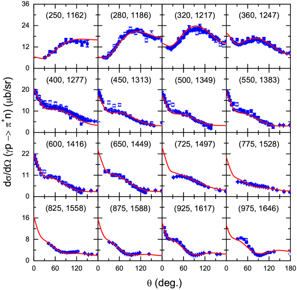
Figure 7: (Color online) Differential cross section for $\gamma p\to\pi^{+}n$ as a function of the scattering angle. The first and second number in each pair of parentheses correspond to the photon laboratory momentum and the $\pi N$ c.m. energy, respectively. Data are taken from Refs. Dugger09 ; Ahrens04 ; SAID .

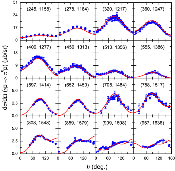
Figure 8: (Color online) Differential cross section for $\gamma p\to\pi^{0}p$ as a function of the scattering angle. The first and second number in each pair of parentheses correspond to the photon laboratory momentum and the $\pi N$ c.m. energy, respectively. Data are taken from Refs. Bartalini05 ; Bartholomy05 ; SAID .

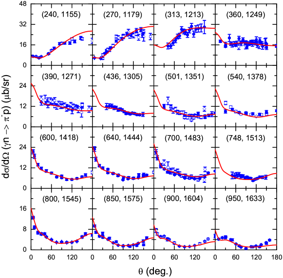
Figure 9: (Color online) Differential cross section for $\gamma n\to\pi^{-}p$ as a function of the scattering angle. The first and second number in each pair of parentheses correspond to the photon laboratory momentum and the $\pi N$ c.m. energy, respectively. Data are taken from Refs. Shafi04 ; SAID .

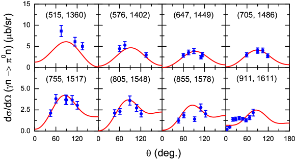
Figure 10: (Color online) Differential cross section for $\gamma n\to\pi^{0}n$ as a function of the scattering angle. The first and second number in each pair of parentheses correspond to the photon laboratory momentum and the $\pi N$ c.m. energy, respectively. Data are taken from Refs. Bacci72 ; Hemmi73 .

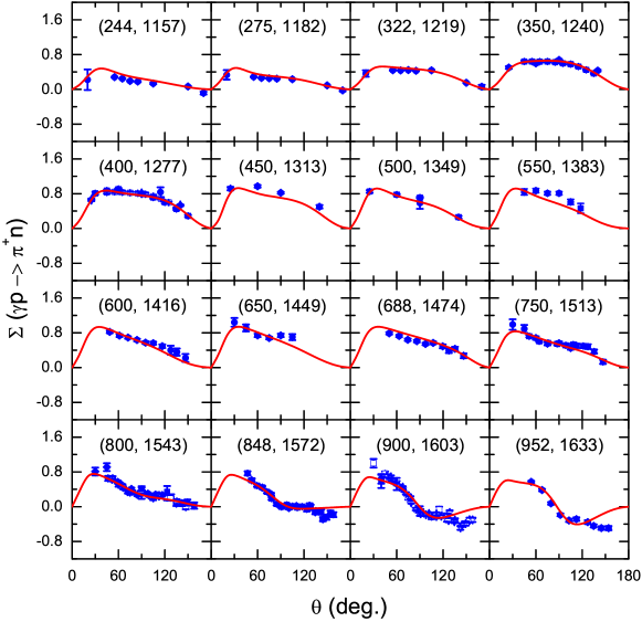
Figure 11: (Color online) Photon spin asymmetry for $\gamma p\to\pi^{+}n$ as a function of the scattering angle. The first and second number in each pair of parentheses correspond to the photon laboratory momentum and the $\pi N$ c.m. energy, respectively. Data are taken from Ref. SAID .

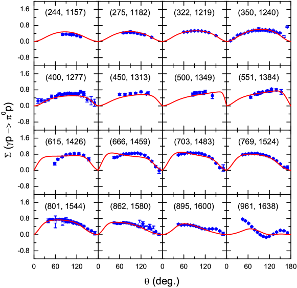
Figure 12: (Color online) Photon spin asymmetry for $\gamma p\to\pi^{0}p$ as a function of the scattering angle. The first and second number in each pair of parentheses correspond to the photon laboratory momentum and the $\pi N$ c.m. energy, respectively. Data are taken from Refs. Bartalini05 ; Elsner09 ; SAID .

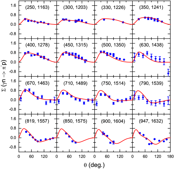
Figure 13: (Color online) Photon spin asymmetry for $\gamma n\to\pi^{-}p$ as a function of the scattering angle. The first and second number in each pair of parentheses correspond to the photon laboratory momentum and the $\pi N$ c.m. energy, respectively. Data are taken from Ref. SAID .

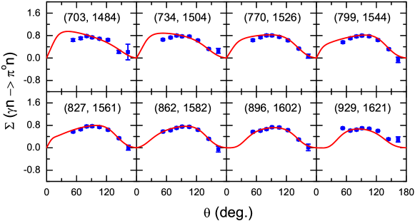
Figure 14: (Color online) Photon spin asymmetry for (quasi-free) $\gamma n\to\pi^{0}n$ as a function of the scattering angle. The first and second number in each pair of parentheses correspond to the photon laboratory momentum and the $\pi N$ c.m. energy, respectively. Data are taken from Ref. Salvo09 .

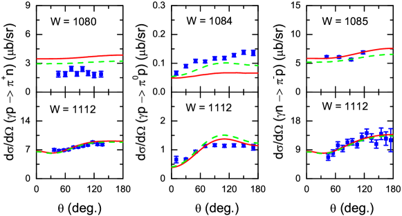
Figure 15: (Color online) Differential cross section for $\gamma p\to\pi^{+}n$, $\gamma p\to\pi^{0}p$ and $\gamma n\to\pi^{-}p$ as a function of the scattering angle. The c.m. energy $W$ is in MeV. The solid curves show the low-energy results from our model. The dashed curves show the results from our calculation where the photoproduction kernel is calculated in particle basis (see text for details). Data are taken from Refs. Korkmaz99 ; Ahrens04 ; Schmidt01 ; Fuchs96 ; SAID ; they were not included in the global fit.

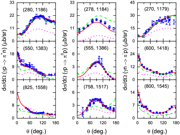
Figure 16: (Color online) Differential cross section for $\gamma p\to\pi^{+}n$, $\gamma p\to\pi^{0}p$ and $\gamma n\to\pi^{-}p$ as a function of the scattering angle. The first and second number in each pair of parentheses correspond to the photon laboratory momentum and the $\pi N$ c.m. energy, respectively. The solid curves show the results from the full calculation. The dotted curves are obtained by switching off the loop integral [the term proportional to the hadronic amplitude $T$ in Eq. (7)]. The dashed curves are obtained by switching off the contact current other than the Kroll-Ruderman term (the term proportional to the meson charge $e_{\pi}$) in $M^{\mu}_{c}$ [cf. Eq. (30)]. Data are taken from Refs. Dugger09 ; Ahrens04 ; Bartalini05 ; Bartholomy05 ; Shafi04 ; SAID .

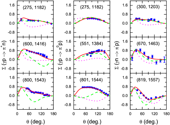
Figure 17: (Color online) Photon spin asymmetry for $\gamma p\to\pi^{+}n$, $\gamma p\to\pi^{0}p$ and $\gamma n\to\pi^{-}p$ as a function of the scattering angle. The first and second number in each pair of parentheses correspond to the photon laboratory momentum and the $\pi N$ c.m. energy, respectively. The solid curves show the results from the full calculation. The dotted curves are obtained by switching off the loop integral [the term proportional to the hadronic amplitude $T$ in Eq. (7)]. The dashed curves are obtained by switching off the contact current other than the Kroll-Ruderman term [the term proportional to the meson charge $e_{\pi}$) in $M^{\mu}_{c}$ (cf. Eq. (30)]. Data are taken from Refs. Bartalini05 ; Elsner09 ; SAID .

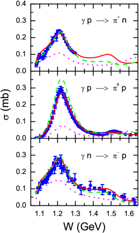
Figure 18: (Color online) Total cross section as a function of the $\pi N$ c.m. energy for $\gamma p\to\pi^{+}n$, $\gamma p\to\pi^{0}p$ and $\gamma n\to\pi^{-}p$. The solid curves show the results from the full calculation. The dotted curves are obtained by switching off the loop integral in Eq. (7). The dashed curves are obtained by switching off the contact current apart from the Kroll-Ruderman term [the term proportional to the meson charge $e_{\pi}$) in $M^{\mu}_{c}$ (cf. Eq. (30)]. Data are taken from Ref. SAID but not included in the fit.

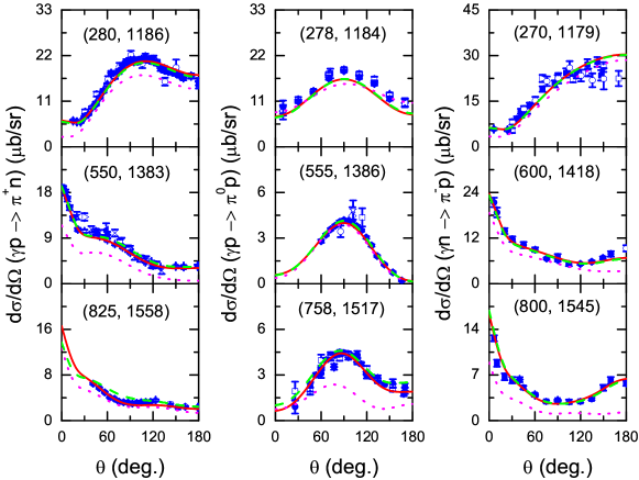
Figure 19: (Color online) Differential cross section for $\gamma p\to\pi^{+}n$, $\gamma p\to\pi^{0}p$ and $\gamma n\to\pi^{-}p$ as a function of the scattering angle. The first and second number in each pair of parentheses correspond to the photon laboratory momentum and the $\pi N$ c.m. energy, respectively. The solid curves show the results from the full calculation. The dotted curves and the dashed curves are obtained by respectively switching off the $\pi\Delta$ loop integral and the $\eta N$ loop integral in Eq. (7). Data are taken from Refs. Dugger09 ; Ahrens04 ; Bartalini05 ; Bartholomy05 ; Shafi04 ; SAID .

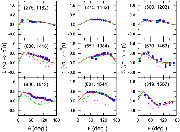
Figure 20: (Color online) Photon spin asymmetry for $\gamma p\to\pi^{+}n$, $\gamma p\to\pi^{0}p$ and $\gamma n\to\pi^{-}p$ as a function of the scattering angle. The first and second number in each pair of parentheses correspond to the photon laboratory momentum and the $\pi N$ c.m. energy, respectively. The solid curves show the results from the full calculation. The dotted curves and the dashed curves are obtained by respectively switching off the $\pi\Delta$ loop integral and the $\eta N$ loop integral in Eq. (7). Data are taken from Refs. Bartalini05 ; Elsner09 ; SAID .

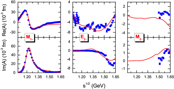
Figure 21: (Color online) Real part and the imaginary part of the multipole amplitudes $M_{1+}$, $E_{2-}$ and $M_{2-}$ for $\gamma N\to\pi N$ with isospin $I=3/2$ as a function of the $\pi N$ c.m. energy. Scattered symbols are amplitudes taken from the George Washington University’s partial-wave analysis Arndt02 .

It was alluded to above in the context of the Bethe-Salpeter equation (13) that the splitting of $T$ into pole and non-pole contributions is no longer unique if the respective pieces are evaluated in a framework that truncates the non-linearities. Owing to this arbitrariness, the pole and non-pole parts of the Jülich model both exhibit spikes in the $P_{11}$ partial wave near the $\pi N$ threshold due to the presence of a nearby unphysical pole in the non-pole transition matrix $X$. This pole in $X$ also affects the pole part of $T$ since the dressed vertices $F$ appearing in the splitting (9) also depend on $X$ via Eq. (11), and one finds that in the sum of pole and non-pole parts, these spikes cancel each other precisely to yield a smooth full $T$-matrix Doring09L . The spikes, therefore, are unphysical artifacts of the particular way the pole and non-pole contributions are calculated in the Jülich model. To circumvent problems of this kind, we have chosen here, in Eq. (7), to work with the full $T$-matrix to describe the hadronic final-state interaction. This, however, does not eliminate completely all numerical difficulties because the $s$-channel contribution in Eq. (7) still involves the dressed $NN\pi$ vertex $F_{s}$ which, as explained, also exhibits the spike by itself. To avoid this problem, we replace here the dressed vertex $F_{s}$ of the Jülich model by the $NN\pi$ vertex obtained within the Feynman prescription for the effective $NN\pi$ interaction Lagrangian ${\cal L}_{NN\pi}$ given in the Appendix employing the physical $NN\pi$ coupling constant and physical nucleon mass.

IV Meson-baryon channels included in the present model

In the present work, as a first step towards a more complete calculation, only the $\pi N$, $\eta N$ and $\pi\Delta$ channels are included as intermediate states in the loop integral in Eq. (7). However, this restriction only concerns the photoproduction sector. In the hadronic sector, all of the five channels $\pi N$, $\eta N$, $\pi\Delta$, $\sigma N$, and $\rho N$ are included via the channels that couple into all of the Jülich $T$-matrices. The main reason we do not include the $\sigma N$ and $\rho N$ channels of the hadronic Jülich model in the present photoproduction calculation is purely practical, namely, the corresponding transition couplings of the photon to these channels would require additional free parameters beyond what we can handle numerically at the moment. Moreover, for the $\rho N$ channel, we expect significant contributions only at energies higher than the c.m. energy of $W=1.65$ GeV considered in the present work.

The channels and intermediate hadrons that contribute explicitly in the present calculation are shown in Fig. 6. As depicted in Fig. 6(a), in addition to the nucleon that is treated as described in Sec. II.2.1, there are eight resonant contributions that enter the $s$-channel term of Eq. (7), i.e., $S_{11}(1535)$, $S_{11}(1650)$, $S_{31}(1620)$, $P_{31}(1910)$, $P_{13}(1720)$, $D_{13}(1520)$, $P_{33}(1232)$, and $D_{33}(1700)$. All of the corresponding hadronic vertices $F_{s}$ and the dressed resonance propagators $S$ are taken from the Jülich $\pi N$ model. The corresponding electromagnetic nucleon-resonance transition vertices $\tilde{J}^{\mu}_{s}$ should be calculated from the analog of Fig. 3(b). However, since the transition currents are all transverse by themselves, the analogs of the longitudinal loops in Fig. 3(b) vanish. Moreover, since we do not consider bare Kroll-Ruderman-type four-point currents for the resonances, we are only left with the bare currents that are given by the corresponding effective Lagrangians (52) and (53) in the Appendix. This is one of the gratifying features of the present formulation that greatly simplifies the calculation of the $s$-channel resonant contributions.

The $\gamma N\to\pi N$ contributions of Fig. 6(b) enter both the Born-type current $B^{\mu}$ and the FSI loop $TG_{0}B^{\mu}_{\textsc{t}}$ of Eq. (7). The contributions of Fig. 6(c) and Fig. 6(d) for $\gamma N\to\eta N$ and $\gamma N\to\pi\Delta$, on the other hand, only enter the FSI loop. For the $t$-channel currents, we include the contributions from the $\pi$, $\rho$, $\omega$, and $a_{1}$ exchanges in the $\gamma N\to\pi N$ channel, from $\rho$ and $\omega$ exchanges in the $\gamma N\to\eta N$ channel and from $\pi$ and $\rho$ exchanges in the $\gamma N\to\pi\Delta$ channel. These diagrams are calculated using the corresponding Lagrangians listed in the Appendix. All the hadronic coupling constants are taken from the Jülich $\pi N$ model Janssen96 ; Schutz98 ; Krehl00 ; Gasparyan03 . The $MM^{\prime}\gamma$ electromagnetic coupling constants are determined from the radiative decay of the relevant mesons in conjunction with SU(3) symmetry considerations. The numerical values of the coupling constants are given the Appendix in connection with their associated interaction Lagrangians. The only adjustable parameters here are the cutoff parameters in the off-shell form factors introduced at the electromagnetic vertices. These form factors are also given in the Appendix.

The only contribution to the $u$-channel amplitude $M^{\mu}_{u}$ considered in the present work is that involving the nucleon (nucleonic current) and $\Delta$ in the intermediate state. Contributions to the $u$-channel from the baryon resonances are not included for consistency reasons since the Jülich hadronic model (and most other existing dynamical models for that matter) does not include the resonance contributions to the $u$-channel except the $\Delta(1232)$ resonance. Apart from an enormous numerical demand in keeping the self-consistency between the $s$- and $u$-channel amplitudes due to the dressed vertices and propagators, the $u$-channel contribution from the baryon resonances are not expected to introduce a significant energy dependence on the resulting reaction amplitude.

We mention here that finally we are left with $38$ adjustable parameters in the present work. Their values will be given and discussed in the next section.

V Results and discussion

The photoproduction reactions of both the neutral and charged pions are considered in the present work up to a c.m. energy of $W=1.65$ GeV. The free parameters of the model as specified in the previous sections are determined by fitting the available differential cross section and photon spin asymmetry data. They are given in Tables 1–5. Here, we note that in the present work, we have attached a momentum cutoff in the loop integral in Eq. (7) of the form $\Lambda^{2}/(\Lambda^{2}+\vec{q}^{\,2})$, where $\vec{q}^{\,2}$ stands for the loop momentum and $\Lambda$ is an adjustable cutoff parameter whose value is also given in Table 1.

The resulting parameters of the effective baryon-resonance electromagnetic transition vertices associated with the current $\tilde{J}^{\mu}_{s}$ as explained in the previous section are summarized in Table 2 for isospin-1/2 resonances and in Table 3 for isospin-3/2 resonances, respectively. We emphasize here that the given coupling constant values should not be confused with the corresponding physical couplings, for they are associated with the current $\tilde{J}^{\mu}_{s}$ [cf. Eq. (7)] which is only a part of the full current $J^{\mu}$ given by Eq. (15). More appropriate (physical) resonance parameters, i.e., masses and coupling strengths, should be associated with the poles of the reaction amplitude, and their corresponding residues, in the complex energy plane. The pole positions and hadronic residues have already been extracted Doring09 in the Jülich hadronic reaction model. Efforts to extract the resonance electromagnetic coupling strengths from the present model are in progress and will be reported elsewhere.

The other adjustable parameters of the model, i.e., the cutoffs in the form factors [Eqs. (54) and (55)] and the parameters $C_{1}$, $C_{2}$, and $\kappa_{0}$ in the nucleon electromagnetic current in Eq. (23) are given in Table 4, while the parameters $\hat{h}$ and $\beta$ in the contact current $M^{\mu}_{c}$ [cf. Eqs. (28) and (30)], are summarized in Table 5. All adjustable parameters were determined by global fits that included all data sets as shown in Figs. 7-14.

The calculated differential cross sections as a function of pion scattering angle in the c.m. frame are shown in Figs. 7–10 for $\gamma p\to\pi^{+}n$, $\gamma p\to\pi^{0}p$, $\gamma n\to\pi^{-}p$, and $\gamma n\to\pi^{0}n$, respectively, together with the corresponding data. Similarly, the calculated photon spin asymmetries are shown in Figs. 11–14. One sees that the overall agreement with the recent experimental data is very good. Some noticeable discrepancies are seen in both the cross sections and beam asymmetries, the latter in $\gamma p\to\pi^{0}p$ and $\gamma p\to\pi^{+}n$ at higher energies. At this point, it is difficult to say whether these discrepancies are due to the lack of higher-spin resonances in the present model or due to the coupled-channels effects other than those from $\eta N$ and $\pi\Delta$ in the photoproduction kernel. In this connection, we mention that the $K\Sigma$ channel with isospin $3/2$ has been incorporated into the Jülich model quite recently RDSHM10 and the inclusion of the isospin-1/2 $K\Sigma$ and $K\Lambda$ channels are currently in progress. The inclusion of the $\rho N$, $\sigma N$ and strangeness channels as well as higher spin resonances such as the $D_{15}$ and $F_{15}$ resonances into our model requires extra free parameters and will be done in future work, which may give us a chance to improve the quality of the present description of the experimental data, especially, in the $W\sim 1.6$ GeV region.

Another multi-channel dynamical model available in the literature which analyzes the pion photoproduction reactions is the EBAC model Diaz08 . This model, based on a unitary transformation method, includes two more resonances than the present model, namely the $D_{15}(1675)$ and $F_{15}(1680)$ resonances; it also includes two more channels in the intermediate state for the photoproduction process, namely the $\rho N$ and $\sigma N$ channels. On the other hand, it analyzes neither the $\gamma n\to\pi^{-}p$ nor the $\gamma n\to\pi^{0}n$ reactions. Although they have considered older data than those in the present work, thus making a close comparison difficult, their results are of comparable fit quality to the present model results overall for both the $\gamma p\to\pi^{0}p$ and $\gamma p\to\pi^{+}n$ reactions. The present results are slightly better at higher energies, especially for photon spin asymmetries for the $\gamma p\to\pi^{0}p$ reaction. Anyway, to achieve the level of the fit quality of the EBAC model results, no spin-5/2 resonances are required in the present model calculation of the pion photoproduction reaction. Further studies are needed to understand the role of those resonances.

At low energies, close to threshold, the pion photo- and electroproduction reactions are nowadays completely understood thanks to ChPT Bernard92 ; BKLM94 . Any meson-exchange dynamical model should, in principle, have built in the constraints of ChPT. It is, however, not a simple task to account for all the constraints dictated by ChPT and, in general, only a few basic constraints are taken into account in practice. Indeed, building in the chiral constraints into meson-exchange models is one of the major improvements needed for these models. The Jülich model uses the phenomenological chiral Lagrangian of Wess and Zumino Wess67 , supplemented by additional Lagrangians for the coupling of $\Delta$, $\omega$, $\eta$, $a_{0}$, and $\sigma$ Krehl00 ; Gasparyan03 , thus honoring some of the chiral constraints. However, it also contains phenomenological form factors which spoil these constraints in general.

Nevertheless, it is interesting to see how the present meson-exchange dynamical model performs at low energies. In Fig. 15, we show our differential cross section results (solid lines) at low energies close to threshold, together with the experimental data. These results, however, were obtained by a refit of the parameters $\hat{h}$ and $\beta$ of the generalized contact current (30), leaving all other parameters unchanged, since it was not possible to obtain reasonable fits using the same constants as for the global fit, in particular, for the $\pi^{0}p$ channel. The refitted values of ($\hat{h}$, $\beta$) are ($12.44$, $0.04$) for the $\pi^{+}n$ channel, ($4.13$, $-1.72$) for the $\pi^{0}p$ channel, and ($6.58$, $-0.83$) for the $\pi^{-}p$ channel, respectively. Comparing with those values listed in Table 5, one sees that these values refitted to the data close to threshold are quite different. This should not be surprising in view of the fact that, in principle, these parameters are energy-dependent functions that are being treated here as constants for simplicity. Near threshold, this restriction becomes especially noticeable. One sees that the overall agreement is reasonable, except for the normalization of the differential cross sections for $\gamma p\to\pi^{0}p$ at $W=1084$ MeV and for $\gamma p\to\pi^{+}n$ at $W=1080$ MeV.

One should also keep in mind that the present calculation is performed in the isospin basis, with averaged nucleon and pion masses of $938.92$ and $138.04$ MeV, respectively, which corresponds to a common threshold energy of about $1077.0$ MeV. This value is about $2$ MeV below the correct threshold value of $1079.1$ MeV for the $\gamma p\to\pi^{+}n$ reaction and might explain, at least in part, why the present calculation over-predicts the cross section at $W=1080$ MeV which is just about $1$ MeV above the correct threshold value. In fact, the dashed curve in the corresponding panel represents the result obtained with the photo-transition amplitudes $F_{s}S\tilde{J}^{\mu}_{s}$ and $B^{\mu}$ [cf. Eqs. (7) and (8)] calculated with the averaged mass of the nucleon and pion set to the neutron and $\pi^{+}$ mass value, respectively, while the hadronic scattering amplitudes are still calculated in the isospin basis. One sees that the agreement with the data is now improved to some extent at $W=1080$ MeV, but not at a higher energy of $W=1112$ MeV. Similarly, the common threshold energy value is about $3.8$ MeV above the correct threshold value of $1073.2$ MeV for the reaction $\gamma p\to\pi^{0}p$. Therefore, in this case we expect the calculated cross section to under-predict the data. Indeed, as can be seen in Fig. 15 (solid curve), this is the case even for the data at $W=1084$ MeV which is about $10.8$ MeV above the correct threshold value. The dashed curve here corresponds to the result analogous to that for the $\pi^{+}n$ final state but with the averaged mass of the nucleon and pion set to the proton and $\pi^{0}$ mass, respectively. One sees a non-negligible improvement in the agreement with the data. In the $\gamma n\to\pi^{-}p$ reaction, the common threshold value is about $0.8$ MeV below the correct value of $1077.8$ MeV and is much smaller than the corresponding differences in the other two reactions just discussed. Therefore, in this case we do not expect that such a small energy difference will affect much the predicted results, especially, if we are at energies not so near the threshold as at $W=1085$ MeV shown in Fig. 15. The dashed curve here is the analog of those for $\pi^{+}p$ and $\pi^{0}p$ for the case of the $\pi^{-}p$ final state, and the effect is negligible as expected. We thus conclude that, apart from the isospin symmetry violation effects arising from the mass differences of pions and nucleons, the present model works remarkably well even at low energies close to threshold. A closer comparison with the low-energy data, however, requires a calculation in the full particle basis. This is especially true for the reaction $\gamma p\to\pi^{0}p$, where it is well known that the near-threshold cross section results from cancelations of competing mechanisms that yield relatively large contributions individually and, therefore, making the prediction of its correct threshold behavior a non-trivial issue Bernard92 ; Bernard:1994gm ; DN10a .

The influence of the loop integral in Eq. (7) and the generalized contact current $M^{\mu}_{c}$ other than the Kroll-Ruderman term in Eq. (8) on the differential cross sections and photon spin asymmetries are illustrated in Figs. 16 and 17, respectively. There, the solid curves correspond to the results of the full calculation. The dotted curves are obtained by switching off the loop integral [the term proportional to the hadronic amplitude $T$ in Eq. (7)]. As one can see, the contribution from the loop integral (which provides the effect of the hadronic final-state interaction) to the cross sections and beam asymmetries is very important showing that it cannot be ignored in these reactions. Note that, in this work, we have the full $T$ in the loop integral of Eq. (7) instead of the non-pole amplitude $X$ employed in the earlier feasibility study of Ref. Haberzettl06 . The dashed curves are obtained by switching off all the terms except the usual Kroll-Ruderman contact term in the generalized contact current $M^{\mu}_{c}$ of Eq. (30). As discussed, these contact terms, unique to the present approach, are required to maintain gauge invariance of the reaction amplitude. Leaving them out, significant effects are seen on the cross sections in both the $\gamma p\to\pi^{+}n$ and $\gamma p\to\pi^{0}p$ processes; the effect in the $\gamma n\to\pi^{-}p$ process is negligible. These gauge-invariance-preserving terms also influence the beam asymmetries at higher energies in a non-trivial way. These interaction-current contributions are seen to be just as important here as they were found to be for $NN$ bremsstrahlung in Ref. NH09 , as discussed in the Introduction (see also the Summary, Sec. VII). The results for both reactions clearly demonstrate that the gauge invariance required for maintaining the internal consistency of the full amplitude in a microscopic model is not purely a theoretical issue but is necessary for the description of the consistent reaction dynamics (see Ref. HN10 for a more detailed discussion on this point).

Figure 18 shows the total cross section as a function of the $\pi N$ c.m. energy for the $\gamma p\to\pi^{+}n$, $\gamma p\to\pi^{0}p$ and $\gamma n\to\pi^{-}p$ reactions. As one can see, the agreement of the full results (solid curves) with the data — the latter taken from Ref. SAID were not included in the global fit — is remarkably good over the entire energy range considered. This figure also shows the influence of the FSI contributions (dotted curves). Again, they are seen to be very important. The influence of the contact terms apart from the Kroll-Ruderman term in the generalized contact current $M^{\mu}_{c}$ [Eq. (30)] is also shown as dashed curves. Here, a significant effect is seen in the $\gamma p\to\pi^{+}n$ reaction in the energy range $W\geq 1.3$ GeV and in the $\gamma p\to\pi^{0}p$ reaction around the energy $W\sim 1.2$ GeV. Note for the $\gamma p\to\pi^{0}p$ reaction, the effect on the total cross section is largely suppressed as compared to that on the differential cross sections (see Fig. 16) due to the phase space factor $\sin(\theta)$.

The effects of the photon coupling to the $\pi\Delta$ and $\eta N$ channels on the cross sections and beam asymmetries are illustrated in Figs. 19 and 20, respectively. There, the solid curves correspond to the full calculation; the dotted curves and dashed curves are obtained by switching off, respectively, the $\pi\Delta$ and $\eta N$ channels in the loop integral in Eq. (7). Note that the threshold energy for opening of the $\pi\Delta$ channel is at $W\cong 1.37$ GeV, while for the $\eta N$ channel is at $W\cong 1.49$ GeV. One sees that the effect of the $\eta N$ channel is practically negligible for cross sections, while it shows some influence on the beam asymmetries at higher energies. The effect of the $\pi\Delta$ channel is significant for reproducing both the cross section and beam asymmetry data at higher energies. The reason for this is that there is an efficient overlap under the loop integral between the generalized contact current $M^{\mu}_{c}$ and the $\pi\Delta\to\pi N$ transition amplitude in the $D_{31}\to S_{31}$ partial-wave state which peaks around $1.6$ GeV due to the strong coupling of the $S_{31}(1620)$ resonance to the $\pi\Delta$ channel. There is also a significant contribution from the $D_{11}\to S_{11}$ partial wave due to the $S_{11}(1535)$ resonance. Here, it should be noted that, since so far the hadronic model parameters in the $\pi\Delta$ channel have not been constrained by the data, the strong coupling of these resonances to the $\pi\Delta$ channel might be an artifact of the model in the hadronic sector. While the present photoproduction reaction may help constrain some of the $\pi\Delta$-channel parameters, more conclusive results can be expected from investigations of two-pion productions $\pi N\to\pi\pi N$ and $\gamma N\to\pi\pi N$.

Motivated by the good agreement of our results with the total and differential cross sections as well as the beam asymmetry data, we have extracted the multipole amplitudes for pion photoproduction and compared them with those from the George Washington University’s partial-wave analysis Arndt02 . In Fig. 21, the results for the multipole amplitudes $M_{1+}$, $E_{2-}$, and $M_{2-}$ from the present calculation (solid curves) are shown together with the results from the SAID analysis Arndt02 . The latter includes not only the cross sections and beam asymmetries but also the target asymmetries and recoil nucleon polarizations as well as some double polarization data into its analysis. We see that the agreement between the two results for the dominant $M_{1+}$ amplitude is quite good. For the smaller $E_{2-}$ amplitude, the agreement is also reasonable, but for the small $M_{2-}$ amplitude there is a considerable disagreement. This illustrates the kind of uncertainties one should expect from the present-type calculations, even though we reproduce the cross sections and beam asymmetries quite nicely. It is clear that in order to extract more reliable multipoles (apart from the dominant ones) from the present model, one needs to include more independent observables to further constrain the model. Actually, the SAID results are also subject to some assumptions in their analysis since at present there exists no complete set of data. Indeed, in order to uniquely determine the amplitude in the present reaction, one requires at least eight independent observables Tabakin (See, also a recent discussion Tiator11 on this issue). In a recent analysis Workman10 , Workman has also investigated the sensitivity of the extracted multipole amplitudes to the accuracy of the data used in their extraction.

VI Uncertainties

Regarding the assessment of theoretical uncertainties of our results, this is very difficult to do in a quantitatively reliable manner within the present phenomenological effective Lagrangian approach because of the absence of a precise ordering scheme for refining the approximations. A procedure was outlined in Ref. RDSHM10 for pion-nucleon scattering that allows one to quantify how the error margins of the data carry over into uncertainties of the extracted parameters of the model approach. A similar approach could be used as well to assess the statistical errors of the photoproduction reaction. However, at present, no quantitative error analysis is available for the Jülich model that we employ here for the hadronic final-state interaction and so we must postpone such an investigation to future work.

In addition to the statistical errors, there are systematic uncertainties inherent in all phenomenological effective Lagrangian approaches that stem from the implementation (or violation) of Lorentz covariance, unitarity, analyticity, and (for photoprocesses) gauge invariance, from the truncation of reaction channels and from how many intermediate resonances are taken into account. For the present approach, we expect the last two sources of uncertainties to be most relevant. Plans are underway to address these issues in future applications by including more channels ($\omega N$, $K\Lambda$, $K\Sigma$) and higher-spin resonances [such as $D_{15}(1675)$ and $F_{15}(1680)$]. However, it may well be that a better understanding of the systematic errors of phenomenological effective Lagrangian approaches can only be obtained by comparing the results of different formalisms. As an example, we point here to the fact that while the present results, by and large, are of a quality similar to that of the EBAC model Diaz08 , we do not need the spin-5/2 resonances employed by that model. This is an important finding in itself since it places the actual role of these resonances in check. However, it may also be an indication that these resonances are needed in the EBAC model to make up for some basic deficiencies of that model, e.g., lack of Lorentz covariance and gauge invariance. In any case, this points to the necessity for further investigating such higher-spin resonances to get a better understanding of the corresponding systematic uncertainties, something we shall do in the future.

VII Summary

We have presented results for the neutral and charged pion photoproduction reactions within a coupled-channels dynamical model in conjunction with the Jülich $\pi N$ hadron-exchange model. The photoproduction amplitude in the present approach satisfies the important properties of analyticity, unitarity and gauge invariance, the latter as dictated by the generalized Ward-Takahashi identity. The overall agreement with the cross section and beam asymmetry data of these reactions is very good in the entire energy range considered. Even at very low energies close to threshold, we have shown that, apart from the isospin-symmetry violation arising from the mass differences of pions and nucleons, the present model works quite well, especially, in view of the delicate cancelations among various competing mechanisms in the $\gamma p\to\pi^{0}p$ reaction near threshold. A closer comparison with the data close to threshold, however, requires a calculation in the particle basis.

The present model includes only the spin-1/2 and -3/2 resonances, showing that, within this model, there is no obvious indication for the need of higher spin resonances — in particular, the $D_{15}(1675)$ and $F_{15}(1680)$ resonances — in the energy range of up to 1.65 GeV to describe the pion photoproduction cross section and beam asymmetry data. In this connection, it is very interesting to extend the present calculation to other (spin) observables in pion photoproduction.

The appearance of the terms in addition to the usual Kroll-Ruderman contact term in the generalized contact current $M^{\mu}_{c}$ [Eq. (30)] is a unique feature of the present model. These terms account for the complicated parts of the interaction current that cannot be taken into account explicitly at present. Our results show that these terms have significant effects on the calculated observables in the present reactions. This means it is very import to take into account properly the gauge-invariance-preserving interaction current for the pion photoproduction processes. The importance of this current corroborates similar findings reported for the $NN$ bremsstrahlung reaction quite recently NH09 , where it was found to be crucial in reproducing the KVI data KVI02 , something which had eluded theoretical attempts for a very long time. The important point here is that this was brought about simply by adding the gauge-invariance-preserving current $M^{\mu}_{c}$, as it is determined here for pion photoproduction, as a novel four-point contact-current mechanism into the description of $NN$ bremsstrahlung, without changing any of the other mechanisms for that reaction. This reciprocal consistency between the current mechanisms employed in the two processes clearly demonstrates that maintaining gauge invariance of the reaction amplitudes, as dictated by the respective generalized Ward-Takahashi identities of all contributing current mechanisms, is not a purely theoretical issue, but an indispensable requirement for a consistent, correct description of the reaction dynamics, with direct consequences for our ability to reproduce the experimental data NH09 ; HN10 .

Apart from the dominant multipole amplitudes, the smaller multipole amplitudes extracted from the present model calculation are shown to be subject to considerable uncertainties, even though the model reproduces quite nicely the recent cross section and beam asymmetry data. It is clear that other independent spin observables need to be included in the analysis to further constrain the model. Note that a unique determination of the multipole amplitudes in pion photoproduction requires, in principle, at least eight independent observables Tabakin which are not available at present.

As we have emphasized in the previous section, the nucleon-resonance electromagnetic transition couplings displayed in Tables II-III are not the physical coupling values and, as such, they are associated only with the present calculation. The appropriate physical electromagnetic couplings should be extracted from the residues associated with the poles of the photoproduction amplitude in the complex-energy plane. The work in this direction is underway and the results will be reported elsewhere.

Finally, we have considered the $\pi N$ c.m. energies up to 1.65 GeV. This upper limit is set by the limitation of the Jülich hadronic model we employed here for the hadronic interactions. To analyze data at higher energies, one needs to include higher-spin baryon resonances, such as $D_{15}(1675)$ and $F_{15}(1680)$. Also, one needs to perhaps also include other meson-baryon channels, such as the $K\Lambda$, $K\Sigma$, and $\omega N$ channels. The $K\Sigma$ channel with isospin $3/2$ has just been incorporated RDSHM10 into the Jülich hadronic model and the inclusion of the strangeness channels with isospin $1/2$ is in progress. The $K\Lambda$ and $K\Sigma$ channels are expected to play a particularly important role in $\eta$ photoproduction DN10 .

In summary, the present work provides a comprehensive treatment of pion photoproduction within a covariant coupled-channels framework based on phenomenological effective Lagrangians. The details of the approach have been constructed HHN2011 with two main goals in mind, namely to preserve the gauge invariance of the current as an off-shell condition and to allow for the consistent incorporation of the hadronic final-state interaction. Overall, our results show very good agreement with the data and they, moreover, show that both properties are indispensable if one wants to provide a quantitatively reliable description of the reaction dynamics of pion photoproduction across the entire resonance region. The extraction of the electromagnetic transition coupling constants for resonances from the residues associated with the poles of the reaction amplitude is currently in progress. It is also straightforward to extend the present approach to the production of other mesons, to strangeness production, and also to the electroproduction of mesons. Tackling all of these reactions is planned for the near future.

*

Appendix A Lagrangians and form factors

We list here the Lagrangians and form factors used in the present work.

The hadronic interaction Lagrangians are:

$${\cal L}_{NN\pi} =-\,g_{NN\pi}{\bar{N}}\left[\gamma_{5}\left(i\lambda+\frac{1-\lambda}{2M_{N}}\,\partial\!\!\!/\right){\bm{\pi}}\cdot{\bm{\tau}}\right]N,$$ (38)

$${\cal L}_{NN\eta} =-\,g_{NN\eta}{\bar{N}}\left[\gamma_{5}\left(i\lambda+\frac{1-\lambda}{2M_{N}}\,\partial\!\!\!/\right)\eta\right]N,$$ (39)

$${\cal L}_{NN\rho} =-\,g_{NN\rho}{\bar{N}}\left[\left(\gamma^{\mu}-\frac{\kappa_{\rho}}{2M_{N}}\sigma^{\mu\nu}\partial_{\nu}\right){\bm{\rho}}_{\mu}\cdot{\bm{\tau}}\right]N,$$ (40)

$${\cal L}_{NN\omega} =-\,g_{NN\omega}{\bar{N}}\left[\left(\gamma^{\mu}-\frac{\kappa_{\omega}}{2M_{N}}\sigma^{\mu\nu}\partial_{\nu}\right)\omega_{\mu}\right]N,$$ (41)

$${\cal L}_{NNa_{1}} =\,g_{NNa_{1}}{\bar{N}}\gamma^{\mu}\gamma_{5}{\bm{\tau}}\cdot\textbf{a}_{1}^{\mu}N,$$ (42)

$${\cal L}_{\Delta N\pi} =\,\frac{g_{\Delta N\pi}}{m_{\pi}}\bar{\Delta}^{\mu}{\bm{T}}\partial_{\mu}{\bm{\pi}}N+{\rm H.c.},$$ (43)

$${\cal L}_{\Delta N\rho} =-\,i\,\frac{g_{\Delta N\rho}}{2m_{N}}{\bar{\Delta}^{\mu}}\gamma^{\nu}\gamma_{5}{\bm{T}}{\bm{\rho}}_{\mu\nu}N+{\rm H.c.},$$ (44)

where $\lambda$ in Eqs. (38) and (39) is the mixing parameter of the pseudoscalar ($\lambda=1$) and pseudovector ($\lambda=0$) type couplings. In this work, $\lambda$ is taken to be zero which means we adopt the pure pseudovector type coupling. The coupling constant values in the above Lagrangians are given in Table 6. All those values have also been used for the hadronic part of the amplitude Krehl00 ; Gasparyan03 employed in the present work.

Table 6: Coupling constant values of the present model fixed from independent sources. The references are shown in the third column. See text for details. $m_{a_{1}}=1260$ MeV.

$g_{NN\pi}$	$13.46$	Schutz98
$g_{NN\eta}$	$4.76$	Schutz98
$g_{NN\rho}$	$3.25$	Janssen96
$\kappa_{\rho}$	$6.10$	Janssen96
$g_{NN\omega}$	$11.76$	Janssen96
$\kappa_{\omega}$	$0.00$	Janssen96
$g_{NNa_{1}}$	$\dfrac{m_{a_{1}}}{m_{\pi}}g_{NN\pi}$	Wess67
$g_{\Delta N\pi}$	$2.13$	Janssen94 ; Janssen942 ; Machleidt87
$g_{\Delta N\rho}$	$-39.10$	Janssen94 ; Janssen942 ; Machleidt87
$g_{\gamma\pi\rho}$	$0.11$	NDHHS99 ; PDG ; Garcilazo93
$g_{\gamma\pi\omega}$	$0.32$	NDHHS99 ; PDG ; Garcilazo93
$g_{\gamma\eta\rho}$	$0.89$	NDHHS99 ; PDG ; NOH08
$g_{\gamma\eta\omega}$	$0.25$	NDHHS99 ; PDG ; NOH08

The electromagnetic interaction Lagrangians for the nucleon and mesons read

$${\cal L}_{NN\gamma}= \,-e\bar{N}\left[\left(\hat{e}\gamma^{\mu}-\frac{\hat{\kappa}}{2M_{N}}\sigma^{\mu\nu}\partial_{\nu}\right)A_{\mu}\right]N,$$ (45)

$${\cal L}_{\gamma\pi\rho}= \;e\frac{g_{\gamma\pi\rho}}{m_{\pi}}\varepsilon_{\alpha\mu\lambda\nu}\left(\partial^{\alpha}A^{\mu}\right)\left(\partial^{\lambda}{\bm{\pi}}\right)\cdot{\bm{\rho}}^{\nu},$$ (46)

$${\cal L}_{\gamma\pi\omega}= \;e\frac{g_{\gamma\pi\omega}}{m_{\pi}}\varepsilon_{\alpha\mu\lambda\nu}\left(\partial^{\alpha}A^{\mu}\right)\left(\partial^{\lambda}\pi_{3}\right)\omega^{\nu},$$ (47)

$${\cal L}_{\gamma\eta\rho}= \;e\frac{g_{\gamma\eta\rho}}{m_{\eta}}\varepsilon_{\alpha\mu\lambda\nu}\left(\partial^{\alpha}A^{\mu}\right)\left(\partial^{\lambda}\eta\right)\rho_{3}^{\nu},$$ (48)

$${\cal L}_{\gamma\eta\omega}= \;e\frac{g_{\gamma\eta\omega}}{m_{\eta}}\varepsilon_{\alpha\mu\lambda\nu}\left(\partial^{\alpha}A^{\mu}\right)\left(\partial^{\lambda}\eta\right)\omega^{\nu},$$ (49)

$$\mathcal{L}_{\gamma\pi\pi}= \;e\left[\left(\partial_{\mu}{\bm{\pi}}\right)\times{\bm{\pi}}\right]_{3}A^{\mu},$$ (50)

$$\mathcal{L}_{\gamma\pi a_{1}}= \;e\,\frac{1}{m_{a_{1}}}F_{\mu\nu}\left[2\left(\partial^{\mu}{\bm{\pi}}\right)\times{\bm{a}}_{1}^{\nu}\,-\,2\left(\partial^{\nu}{\bm{\pi}}\right)\times{\bm{a}}_{1}^{\mu}\right.$$

$$+\left.{\bm{\pi}}\times{\bm{a}}_{1}^{\mu\nu}\right]_{3},$$ (51)

where $e$ stands for the elementary charge unit, and $\hat{e}\equiv(1+\tau_{3})/2$ and $\hat{\kappa}\equiv\kappa_{p}(1+\tau_{3})/2+\kappa_{n}(1-\tau_{3})/2$, with the anomalous magnetic moments $\kappa_{p}=1.793$ of the proton and $\kappa_{n}=-1.913$ of the neutron; $F_{\mu\nu}\equiv\partial_{\mu}A_{\nu}-\partial_{\nu}A_{\mu}$ with $A_{\mu}$ denoting the electromagnetic field and ${\bm{a}}_{1}^{\mu\nu}\equiv\partial^{\mu}{\bm{a}}_{1}^{\nu}-\partial^{\nu}{\bm{a}}_{1}^{\mu}$; $\varepsilon_{\alpha\mu\lambda\nu}$ is the totally antisymmetric Levi-Civita tensor with $\varepsilon^{0123}=+1$. The meson-meson electromagnetic transition coupling constants in the above Lagrangians are given in Table 6. Following Ref. NDHHS99 , they are fixed from the decay PDG of the $\rho$ and $\omega$ meson into the $\gamma\pi^{0}$ and $\gamma\eta$ channels, respectively. The signs of the coupling constants $g_{\gamma\pi\rho}$ and $g_{\gamma\pi\omega}$ are consistent with those determined from the study of pion photoproduction in the 1-GeV region Garcilazo93 . The signs of $g_{\gamma\eta\rho}$ and $g_{\gamma\eta\omega}$ are inferred from the flavor SU(3) symmetry considerations as used in Ref. NOH08 .

The resonance-nucleon photo-transition Lagrangians are

$$\mathcal{L}^{1\!/2\pm}_{RN\gamma}= \;e\frac{g_{RN\gamma}^{(1)}}{2M_{N}}\bar{R}\Gamma^{(\mp)}\sigma_{\mu\nu}\left(\partial^{\nu}A^{\mu}\right)N+{\rm H.c.},$$ (52)

$$\mathcal{L}^{3\!/2\pm}_{RN\gamma}= \,-ie\frac{g^{(1)}_{RN\gamma}}{2M_{N}}{\bar{R}^{\mu}}\gamma_{\nu}\Gamma^{(\pm)}F^{\mu\nu}N$$

$$\,+e\frac{g^{(2)}_{RN\gamma}}{4M^{2}_{N}}\bar{R}^{\mu}\Gamma^{(\pm)}F^{\mu\nu}\partial_{\nu}N+{\rm H.c.},$$ (53)

where $\Gamma^{(+)}\equiv\gamma_{5}$ and $\Gamma^{(-)}\equiv 1$; the superscript of $\mathcal{L}_{RN\gamma}$ denotes the spin and parity of the resonance $R$.

For the $s$-channel $NN\pi$ vertex and the $u$-channel $NN\pi$ and $\Delta N\pi$ vertices, the following covariant form factor is employed in our model:

$$F_{B}(p^{2})=\left(\frac{\Lambda_{B}^{4}}{\Lambda_{B}^{4}+\left(m_{B}^{2}-p^{2}\right)^{2}}\right)^{n},$$ (54)

where $p$ and $m_{B}$ denote the four-momentum and mass of the off-shell baryon, respectively. The exponent $n$ is taken to be $2$ for $\Delta N\pi$ vertex and $1$ for $NN\pi$ vertex. The parameter $\Lambda_{B}$ is determined by fitting to the data and it is listed in Table 1.

For the hadronic vertices in the $t$-channel diagrams, the following covariant form factor is included

$$F_{\alpha}(q^{2})=\left(\frac{\Lambda_{\alpha}^{2}-m_{\alpha}^{2}}{\Lambda_{\alpha}^{2}-q^{2}}\right)^{n_{\alpha}},$$ (55)

where $\alpha$ stands for the off-shell meson ($\alpha=\pi$, $\rho$, $\omega$, $a_{1}$); $q$ and $m_{\alpha}$ denote the four-momentum and mass of the off-shell meson, respectively. The exponent $n_{\alpha}$ is taken to be $1$ for $\alpha=\pi$ Janssen94 ; Janssen942 and $2$ for other mesons Machleidt87 . We use the same cutoff $\Lambda_{v}$ for $\rho$, $\omega$ and $a_{1}$ mesons in order to reduce the number of model parameters. The values of the cutoff parameters $\Lambda_{\pi}$ and $\Lambda_{v}$ are determined by fitting to the data; they are listed in Table 1.

Note that the gauge invariance feature of our photoproduction amplitude is independent of the specific form of the form factors.

References

- (1) E. Klempt and J.M. Richard, Rev. Mod. Phys. 82, 1095 (2010).
- (2) R.E. Cutkosky, C.P. Forsyth, R.E. Hendrick, and R.L. Kelly, Phys. Rev. D 20, 2839 (1979).
- (3) R.E. Cutkosky, C.P. Forsyth, J.B. Babcock, R.L. Kelly, and R.E. Hendrick, in Baryons 1980, Proceedings of the IVth International Conference on Baryon Resonances, ed. N. Isgur (University of Toronto, 1980), p. 19.
- (4) G. Höhler, Pion-Nucleon Scattering, Landolt-Börnstein Vol. I/9b2, ed. H. Schopper (Springer, Berlin, 1983).
- (5) G. Höhler, Newsletter 9, 1 (1993).
- (6) R.A. Arndt, I.I. Strakovsky, R.L. Workman, and M. Pavan, Phys. Rev. C 52, 2120 (1995).
- (7) R.A. Arndt, W.J. Briscoe, I.I. Strakovsky, and R.L. Workman, Phys. Rev. C 66, 055213 (2002).
- (8) R.A. Arndt, W.J. Briscoe, I.I. Strakovsky, and R.L. Workman, Phys. Rev. C 74, 045205 (2006).
- (9) V. Bernard, N. Kaiser, J. Gasser, and U.G. Meißner, Phys. Lett. B 268, 291 (1991).
- (10) V. Bernard, N. Kaiser, and U.-G. Meißner, Nucl. Phys. B 383, 442 (1992).
- (11) V. Bernard, N. Kaiser, and U.-G. Meißner, Z. Phys. C 70, 483 (1996).
- (12) V. Bernard, Prog. Part. Nucl. Phys. 60, 82 (2008).
- (13) B. Borasoy, P.C. Bruns, U.-G. Meißner, and R. Nissler, Phys. Rev. C 72, 065201 (2005).
- (14) B. Borasoy, P.C. Bruns, U.-G. Meißner, and R. Nissler, Eur. Phys. J. A 34, 161 (2007).
- (15) D. Ruic, M. Mai, and U.-G. Meißner, Phys. Lett. B 704, 659 (2011).
- (16) M. Döring and K. Nakayama, Phys. Lett. B 683, 145 (2010).
- (17) N. Kaiser, T. Waas, and W. Weise, Nucl. Phys. A 612, 297 (1997).
- (18) J.C. Nacher, E. Oset, H. Toki, and A. Ramos, Phys. Lett. B 461, 299 (1999).
- (19) E. Marco, S. Hirenzaki, E. Oset, and H. Toki, Phys. Lett. B 470, 20 (1999).
- (20) J. Caro Ramon, N. Kaiser, S. Wetzel, and W. Weise, Nucl. Phys. A 672, 249 (2000).
- (21) U.-G. Meißner and J.A. Oller, Nucl. Phys. A 673, 311 (2000).
- (22) A. Gasparyan and M.F.M. Lutz, Nucl. Phys. A 848, 126 (2010).
- (23) N. Kaiser, P.B. Siegel, and W. Weise, Phys. Lett. B 362, 23 (1995).
- (24) E.E. Kolomeitsev and M.F.M. Lutz, Phys. Lett. B 585, 243 (2004).
- (25) S. Sarkar, E. Oset, and M.J. Vincente Vacas, Nucl. Phys. A 750, 294 (2005).
- (26) M. Döring, Nucl. Phys. A 786, 164 (2007).
- (27) D. Jido, M. Döring, and E. Oset, Phys. Rev. C 77, 065207 (2008).
- (28) P.C. Bruns, M. Mai, and U.-G. Meißner, Phys. Lett. B 697, 254 (2011).
- (29) S. Ceci, M. Döring, C. Hanhart, S. Krewald, U.-G. Meißner, and A. Švarc, Phys. Rev. C 84, 015205 (2011).
- (30) C. Schütz, J.W. Durso, K. Holinde, and J. Speth, Phys. Rev. C 49, 2671 (1994).
- (31) C. Schütz, J. Haidenbauer, J. Speth, and J.W. Durso, Phys. Rev. C 57, 1464 (1998).
- (32) O. Krehl, C. Hanhart, S. Krewald, and J. Speth, Phys. Rev. C 62, 025207 (2000).
- (33) A.M. Gasparyan, J. Haidenbauer, C. Hanhart, and J. Speth, Phys. Rev. C 68, 045207 (2003).
- (34) M. Döring, C. Hanhart, F. Huang, S. Krewald, U.-G. Meißner, and D. Rönchen, Nucl. Phys. A 851, 58 (2011).
- (35) M. Döring, J. Haidenbauer, U.-G. Meißner, and A. Rusetsky, arXiv: 1108.0676 [hep-lat].
- (36) Y. Surya and F. Gross, Phys. Rev. C 53, 2422 (1996).
- (37) G.Y. Chen, S.S. Kamalov, S.N. Yang, D. Drechsel, and L. Tiator, Phys. Rev. C 76, 035206 (2007).
- (38) A. Matsuyama, T. Sato, and T.-S.H. Lee, Phys. Rept. 439, 193 (2007) and references therein.
- (39) B. Juliá-Díaz, T.-S.H. Lee, A. Matsuyama, T. Sato, and L.C. Smith, Phys. Rev. C 77, 045205 (2008).
- (40) B. Juliá-Díaz, H. Kamano, T.-S.H. Lee, A. Matsuyama, T. Sato, and N. Suzuki, Phys. Rev. C 80, 025207 (2009).
- (41) H. Kamano, B. Juliá-Díaz, T.-S.H. Lee, A. Matsuyama, and T. Sato, Phys. Rev. C 80, 065203 (2009).
- (42) V. Shklyar, G. Penner, and U. Mosel, Eur. Phys. J. A 21, 445 (2004).
- (43) G. Penner and U. Mosel, Phys. Rev. C 66, 055212 (2002).
- (44) A. Usov and O. Scholten, Phys. Rev. C 72, 025205 (2005).
- (45) A.V. Sarantsev, V.A. Nikonov, A.V. Anisovich, E. Klempt, and U. Thoma, Eur. Phys. J. A 25, 441 (2005).
- (46) A.V. Anisovich, E. Klempt, V.A. Nikonov, A.V. Sarantsev, and U. Thoma, Eur. Phys. J. A 47, 27 (2010).
- (47) D. Drechsel, S.S. Kamalov, and L. Tiator, Eur. Phys. J. A 34, 69 (2007).
- (48) L. Tiator, D. Drechsel, S.S. Kamalov, and M. Vanderhaeghen, arXiv: 1109.6745 [nucl-th].
- (49) H. Haberzettl, K. Nakayama, and S. Krewald, Phys. Rev. C 74, 045202 (2006).
- (50) H. Haberzettl, F. Huang, and K. Nakayama, Phys. Rev. C 83, 065502 (2011).
- (51) For TOPT see, e.g., S.S. Schweber, “An Introduction to Relativistic Quantum Field Theory” (Harper&Row, 1961; reprinted by Dover, 2005).
- (52) J. Wess and B. Zumino, Phys. Rev. 163, 1727 (1967).
- (53) U.-G. Meißner, Phys. Rept. 161, 213 (1988).
- (54) M. Döring, C. Hanhart, F. Huang, S. Krewald, and U.-G. Meißner, Phys. Lett. B 681, 26 (2009).
- (55) M. Döring, C. Hanhart, F. Huang, S. Krewald, and U.-G. Meißner, Nucl. Phys. A 829, 170 (2009).
- (56) H. Haberzettl, Phys. Rev. C 56, 2041 (1997).
- (57) E. Kazes, Nuovo Cimento 13, 1226 (1959).
- (58) V. Pascalutsa and J.A. Tjon, Phys. Rev. C 70, 035209 (2004).
- (59) G.L. Caia, V. Pascalutsa, J.A. Tjon, and L.E. Wright, Phys. Rev. C 70, 032201(R) (2004).
- (60) G.L. Caia, L.E. Wright, and V. Pascalutsa, Phys. Rev. C 72, 035203 (2005).
- (61) F. Gross and D.O. Riska, Phys. Rev. C 36, 1928 (1987).
- (62) C.H.M. van Antwerpen and I.R. Afnan, Phys. Rev. C 52, 554 (1995).
- (63) A.N. Kvinikhidze, B. Blankleider, E. Epelbaum, C. Hanhart, and M.P. Valderrama, Phys. Rev. C 80, 044004 (2009).
- (64) J.C. Ward, Phys. Rev. 78, 182 (1950); Y. Takahashi, Nuovo Cimento 6, 370 (1957).
- (65) K. Nakayama and H. Haberzettl, Phys. Rev. C 80, 051001(R) (2009).
- (66) H. Haberzettl and K. Nakayama, arXiv: 1011.1927 [nucl-th].
- (67) H. Huisman et al., Phys. Rev. C 65, 031001(R) (2002).
- (68) M. Gell-Mann and M.L. Goldberger, Phys. Rev. 96, 1433 (1954).
- (69) J.S. Ball and T.W. Chiu, Phys. Rev. D 22, 2542 (1980).
- (70) V.G. Kadyshevsky, Nucl. Phys. B 6, 125 (1968).
- (71) G. Janssen, K. Holinde, and J. Speth, Phys. Rev. C 54, 2218 (1996).
- (72) M. Dugger et al., CLAS Collaboration, Phys. Rev. C 79, 065206 (2009).
- (73) J. Ahrens et al., GDH and A2 Collaboration, Eur. Phys. J. A 21, 323 (2004).
- (74) CNS Data Analysis Center, The George Washington University, http://gwdac.phys.gwu.edu/.
- (75) O. Bartalini et al., GRAAL Collaboration, Eur. Phys. J. A 26, 399 (2005).
- (76) O. Bartholomy et al., CB-ELSA Collaboration, Phys. Rev. Lett. 94, 012003 (2005).
- (77) A. Shafi et al., Crystal Ball Collaboration, Phys. Rev. C 70, 035204 (2004).
- (78) C. Bacci et al., Phys. Lett. B 39, 559 (1972).
- (79) Y. Hemmi et al., Nucl. Phys. B 55, 333 (1973).
- (80) D. Elsner et al., CB-ELSA Collaboration and TAPS Collaboration, Eur. Phys. J. A 39, 373 (2009).
- (81) R. Di Salvo et al., GRAAL Collaboration, Eur. Phys. J. A 42, 151 (2009).
- (82) V. Bernard, N. Kaiser, T.-S.H. Lee, and U.-G. Meißner, Phys. Rept. 246, 315 (1994).
- (83) E.J. Korkmaz et al., Phys. Rev. Lett. 83, 3609 (1999).
- (84) A. Schmidt et al., Phys. Rev. Lett. 87, 232501 (2001).
- (85) M. Fuchs et al., Phys. Lett. B 368, 20 (1996).
- (86) M. Döring and K. Nakayama, Eur. Phys. J. A 43, 83 (2010).
- (87) W.T. Chiang and F. Tabakin, Phys. Rev. C 55, 2054 (1997).
- (88) L. Tiator, arXiv: 1109.0608 [nucl-th].
- (89) R.L. Workman, Phys. Rev. C 83, 035201 (2011).
- (90) G. Janssen, K. Holinde, and J. Speth, Phys. Rev. Lett. 73, 1332 (1994).
- (91) G. Janssen, K. Holinde, and J. Speth, Phys. Rev. C 49, 2763 (1994).
- (92) R. Machleidt, K. Holinde, and Ch. Elster, Phys. Rept. 149, 1 (1987).
- (93) K. Nakayama, J.W. Durso, J. Haidenbauer, C. Hanhart, and J. Speth, Phys. Rev. C 60, 055209 (1999).
- (94) Particle Data Group, J. Phys. G 37, 075021 (2010).
- (95) H. Garcilazo and E. Moya de Guerra, Nucl. Phys. A 562, 521 (1993).
- (96) K. Nakayama, Yongseok Oh, and H. Haberzettl, J. Kor. Phys. Soc. 59, 224 (2011) [arXiv: 0803.3169 [hep-ph]].