Studying Deeply Virtual Compton Scattering with Neural Networks

Abstract

Neural networks are utilized to fit Compton form factor $\mathcal{H}$ to HERMES data on deeply virtual Compton scattering off unpolarized protons. We used this result to predict the beam charge-spin assymetry for muon scattering off proton at the kinematics of the COMPASS II experiment.

1 Introduction

Deeply virtual Compton Scattering (DVCS) is recognized as the theoretically cleanest process for accessing generalized parton distributions (GPDs) [1, 2, 3], which describe the three-dimensional structure of nucleon in terms of partonic degrees of freedom. Determination of GPDs, beside improving our general understanding of QCD dynamics, allows to address important questions such as the partonic decomposition of the nucleon spin [4] and characterization of multiple-hard reactions in proton-proton collisions at LHC collider [5]. Concerning the latter, GPD-describable non-trivial transversal structure of proton, such as the correlation between parton’s longitudinal momentum fraction and its transversal distance is already finding its way in popular event generators, such as PYTHIA [6].

Similarly to extraction of normal parton distribution functions (PDFs), extraction of GPDs can be performed by global model or local fits to available data [7, 8, 9, 10, 11, 12]. However, compared to global PDF fits, extracting GPDs from data is a much more intricate task and model ambiguities are much larger. Due to the facts that GPDs cannot be fully constrained from data and that they depend at the input scale on three variables, the space of possible functions, although restricted by GPD constraints, is huge. As a result, the theoretical systematic error induced by the choice of the fitting model is much more serious than in the PDF case, where the model functions depend at the input scale only on one variable, namely, the longitudinal momentum fraction $x$.

Here we report on some results obtained using alternative approach [13], in which neural networks are used in place of specific models. This essentially eliminates the problem of model dependence and, as an additional advantage, facilitates a convenient method to propagate uncertainties from experimental measurements to the final result. Our approach is mostly similar to the one already employed for $F_{2}$ structure function and PDF extraction [14, 15, 16] and will be shortly described in the next section. To reduce the mathematical complexity of the problem we have fitted not the GPDs itself, but the dominant Compton form factor (CFF) $\mathcal{H}(x_{B},t)$, depending on Bjorken variable $x_{B}$ and momentum transfer $t$. At leading order, the imaginary part of this CFF is related to the corresponding GPD $H(x,\xi,t)$ at the cross-over line $x=\xi$:

$$\operatorname{\mathfrak{Im}}{\cal H}(x_{B}=\frac{2\xi}{1+\xi},t)\stackrel{{\scriptstyle\rm LO}}{{=}}\pi\bigg{(}H(\xi,\xi,t)-H(-\xi,\xi,t)\bigg{)}\;,$$ (1)

so knowledge of CFF $\mathcal{H}$ provides us with direct information about the proton structure.

2 The Method of Fitting Data with Neural Networks

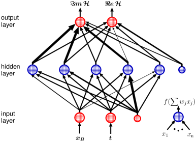
Figure 1: A neural network parametrization of the complex-valued CFF $\mathcal{H}(x_{B},t)$. Each blob symbolizes a neuron and thickness of arrows represents the strengths of weights $w_{j}$.

The neural network type used in this work, known as multilayer perceptron, is a mathematical structure consisting of a number of interconnected “neurons” organized in several layers. It is schematically shown on Figure 1, where each blob symbolizes a single neuron. Each neuron has several inputs and one output. The value at the output is given as a function $f(\sum_{j}w_{j}x_{j})$ of a sum of values at inputs $x_{1},x_{2},\cdots$, each weighted by a certain number $w_{j}$. For activation function $f(x)$ we employed logistic sigmoid function

$$f(x)=1/(1+\exp(-x))$$

for neurons in inner (“hidden”) layer, while for input and output layers we used the identity function.

By iterating over the following steps the network is trained, i.e., it “learns” how to describe a certain set of data points:

1. Kinematic values (two in our case: $x_{B}$ and $t$) of the first data point are presented to two input-layer neurons

2. These values are then propagated through the network according to values of weights $w_{j}$. In the first iteration, weights are set to some random value.

3. As a result, the network produces some resulting values of output in its output-layer neurons. Here we have two: $\operatorname{\mathfrak{Im}}\mathcal{H}$ and $\operatorname{\mathfrak{Re}}\mathcal{H}$. Obviously, after the first iteration, these will be some random functions of the input kinematic values: $\operatorname{\mathfrak{Im}}\mathcal{H}(x_{B},t)$ and $\operatorname{\mathfrak{Re}}\mathcal{H}(x_{B},t)$.

4. Using these values of CFF(s), the observable corresponding to the first data point is calculated and it is compared to actually measured value, with squared error used for building the standard $\chi^{2}$ function.

5. The obtained error is then used to modify the network: It is propagated backwards through the layers of the network and each weight is adjusted such that this error is decreased.

6. This procedure is then repeated with the next data point, until the whole training set is exhausted.

This sequence of steps is repeated until the network is capable to describe experimental data with a sufficient accuracy. To guard against overfitting the data (“fitting to the noise”), one (randomly chosen) subset of data is not used for training but only for monitoring the progress and stopping the training when error of network description of this data starts to increase significantly. This ensures that resulting neural network represents a function which is not too complex and which is thus expected to provide a reasonable estimate of the actual underlying physical law.

To propagate experimental uncertainties into the final result we used the “Monte Carlo” method [17] where neural networks are not trained on actual data but on a collection of “replica data sets”. These sets are obtained from original data by generating random artificial data points according to Gaussian probability distribution with a width defined by the error bar of experimental measurements. Taking a large number $N_{rep}$ of such replicas, the resulting collection of trained neural networks $\mathcal{H}^{(1)},\ldots,\mathcal{H}^{(N_{rep})}$ defines a probability distribution $\mathcal{P}[\mathcal{H}]$ of the represented CFF $\mathcal{H}(x_{B},t)$ and of any functional $\mathcal{F}[\mathcal{H}]$ thereof. Thus, the mean value of such a functional and its variance are [17, 14]

$$\Big{\langle}\mathcal{F}[\mathcal{H}]\Big{\rangle} =\int\mathcal{D}\mathcal{H}\>\mathcal{P}[\mathcal{H}]\,\mathcal{F}[\mathcal{H}]=\frac{1}{N_{rep}}\sum_{k=1}^{N_{rep}}\mathcal{F}[\mathcal{H}^{(k)}]\;,$$ (2)

$$\Big{(}\Delta\mathcal{F}[\mathcal{H}]\Big{)}^{2} =\Big{\langle}\mathcal{F}[\mathcal{H}]^{2}\Big{\rangle}-\Big{\langle}\mathcal{F}[\mathcal{H}]\Big{\rangle}^{2}\;.$$ (3)

More details about our procedure can be found in [13].

3 First results

We now present neural network fits [13] to two sets of HERMES collaboration measurements [18] of leptoproduction of a real photon by scattering leptons off unpolarized protons (of which DVCS is a subprocess). One set consists of 18 measurements of the first sine harmonic $A_{LU}^{\sin\phi}$ of the beam spin asymmetry (BSA)

$$BSA\equiv\frac{{\rm d}\sigma_{e^{\uparrow}}-{\rm d}\sigma_{e^{\downarrow}}}{{\rm d}\sigma_{e^{\uparrow}}+{\rm d}\sigma_{e^{\downarrow}}}\sim A_{LU}^{\sin\phi}\sin\phi\;,$$ (4)

(where $\phi$ is the azimuthal angle in the so-called Trento convention), while in the other set there are 18 measurements of the first cosine harmonic $A_{C}^{\cos\phi}$ of the beam charge asymmetry (BCA)

$$BCA\equiv\frac{{\rm d}\sigma_{e^{+}}-{\rm d}\sigma_{e^{-}}}{{\rm d}\sigma_{e^{+}}+{\rm d}\sigma_{e^{-}}}\sim A_{C}^{\cos 0\phi}+A_{C}^{\cos\phi}\cos\phi\;.$$ (5)

Both sets cover the identical kinematic region

$$0.05<x_{B}<0.24\,,\quad 0.02<-t/{\rm GeV}^{2}<0.46\,,\quad\mbox{and}\quad 1.2<\mathcal{Q}^{2}/{\rm GeV}^{2}<6.11\,,$$

and in this region BSA and BCA are determined essentially by the imaginary and the real part of the Compton form factor $\mathcal{H}$ [19], respectively, so we ignored other CFFs. Furthermore, in this region the dependence of $\mathcal{H}$ on the photon virtuality $\mathcal{Q}^{2}$ is weak and, therefore, we neglected it for simplicity. Thus, at present, just a single CFF $\mathcal{H}(x_{B},t)$, or two real-valued functions $\operatorname{\mathfrak{Im}}\mathcal{H}(x_{B},t)$ and $\operatorname{\mathfrak{Re}}\mathcal{H}(x_{B},t)$, are extracted from data by neural networks.

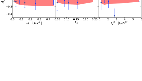
Figure 2: First cosine harmonic of beam charge asymmetry $A_{C}^{\cos\phi}$ (5) and first sine harmonic of beam spin asymmetry $A_{LU}^{\sin\phi}$ (4) resulting from neural network fit, shown together with data [18], used for training.

We fitted this data using the method described in the previous section where we constructed 50 neural networks with architecture (2-13-2), i.e., with two input neurons (for two kinematic variables $x_{B}$ and $t$), 13 neurons in the hidden layer (where we convinced ourselves that adding or removing few neurons doesn’t significantly change the results), and 2 output neurons (representing $\operatorname{\mathfrak{Im}}\mathcal{H}(x_{B},t)$ and $\operatorname{\mathfrak{Re}}\mathcal{H}(x_{B},t)$). On Figure 2 we show the fit quality by presenting the data used for training together with the description of this data by the final set of 50 neural networks, using relations (2) and (3).

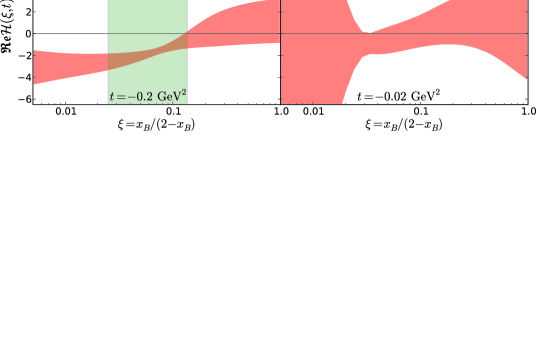
Figure 3: Neural network extraction of $\operatorname{\mathfrak{Im}}{\cal H}(x_{\rm Bj},t)$ and $\operatorname{\mathfrak{Re}}{\cal H}(x_{\rm Bj},t)$ from HERMES BCA and BSA [18] data. Actual data region is shown as vertical band in the middle of the left two panels. Outside of this band and on the whole of the right two panels, neural networks are extrapolating from the data.

CFF $\mathcal{H}$ itself, which is our main result, is displayed in Figure 3, where $\operatorname{\mathfrak{Im}}\mathcal{H}$ (upper panels) and $\operatorname{\mathfrak{Re}}\mathcal{H}$ (lower panels) are separately plotted. One notices that in the kinematic region of the measured data (this is roughly the middle vertical third of the left panels), where neural networks are interpolating the data, CFF $\mathcal{H}$ is estimated with a reasonably small uncertainty. However, as one starts to extrapolate the fitted CFF $\mathcal{H}$ outside of the data region (left and right thirds of left panels and the whole of the right panels), the neural network parameterization of CFF $\mathcal{H}$ is very unconstrained. This is particularly visible in the right panels, illustrating the difficulty of a model-independent extrapolation towards $t=0$, which is a limit of particular interest for hadron structure studies.

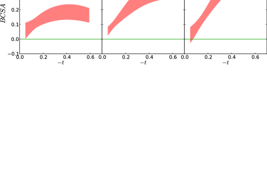
Figure 4: Predictions of neural network fits for beam charge-spin asymmetry (6) in COMPASS II kinematics ($E_{\mu}=160\,{\rm GeV}$, $\phi=0$).

Finally, as an example of a proper prediction coming from our analysis we plot in Figure 4 the beam charge-spin asymmetry (BCSA),

$$BCSA\equiv\frac{{\rm d}\sigma_{\mu^{\downarrow+}}-{\rm d}\sigma_{\mu^{\uparrow-}}}{{\rm d}\sigma_{\mu^{\downarrow+}}+{\rm d}\sigma_{\mu^{\uparrow-}}}\;,$$ (6)

as a function of momentum transfer $t$, for several kinematic points that are characteristic for the COMPASS II experiment of scattering muons and antimuons off proton target (where the muon is taken to be massless and the polarization is set equal to 0.8). This experiment was chosen because its kinematics overlap with that of the HERMES data used for neural network training. Hence these predictions represent partly interpolation and partly extrapolation of HERMES data, thus testing this whole approach in a nontrivial way.

4 Conclusions and outlook

By explicit extraction of Compton form factor $\mathcal{H}$ from HERMES data on beam spin and charge asymmetries we demonstrated that neural networks can be a powerful tool for studying hadron structure. They can interpolate experimental data in an unbiased way, eliminating thus the systematic error introduced by choosing a specific fitting function in the standard model-fitting approaches. Since GPDs and CFFs are multivariate functions, this advantage is much more pronounced than in PDF fitting, where PDFs on the input scale depend only on a single variable. Still, this feature of neural network approach cuts both ways: unbiased fitting of GPDs and CFFs to the precision of the present PDF fits would require orders of magnitude more data then presently available — to cover the larger dimension of the kinematic space. To overcome this problem, one may deliberately introduce some biases and constraints on neural networks, especially those that correspond to certain well established properties of represented functions (e.g. dispersion relations between imaginary and real parts of CFFs [20, 7, 21, 22]). Furthermore, one could view neural network fits as intermediate results and use them as a tool for model-dependent studies.

References

- [1] Müller D, Robaschik D, Geyer B, Dittes F M and Hořejši J 1994 Fortschr. Phys. 42 101 (Preprint hep-ph/9812448)
- [2] Radyushkin A V 1996 Phys. Lett. B380 417–425 (Preprint hep-ph/9604317)
- [3] Ji X D 1997 Phys. Rev. D55 7114–7125 (Preprint hep-ph/9609381)
- [4] Ji X D 1997 Phys. Rev. Lett. 78 610–613 (Preprint hep-ph/9603249)
- [5] Diehl M and Schäfer A 2011 Phys. Lett. B698 389–402 (Preprint 1102.3081)
- [6] Corke R and Sjöstrand T 2011 JHEP 05 009 (Preprint 1101.5953)
- [7] Kumerički K, Müller D and Passek-Kumerički K 2008 Nucl. Phys. B794 244–323 (Preprint hep-ph/0703179)
- [8] Guidal M 2008 Eur. Phys. J. A37 319–332 (Preprint 0807.2355)
- [9] Kumerički K and Müller D 2010 Nucl. Phys. B841 1–58 (Preprint 0904.0458)
- [10] Guidal M and Moutarde H 2009 Eur. Phys. J. A42 71–78 (Preprint 0905.1220)
- [11] Guidal M 2010 Phys. Lett. B689 156–162 (Preprint 1003.0307)
- [12] Moutarde H 2009 Phys. Rev. D79 094021 (Preprint 0904.1648)
- [13] Kumerički K, Müller D and Schäfer A 2011 JHEP 07 073 (Preprint 1106.2808)
- [14] Forte S, Garrido L, Latorre J I and Piccione A 2002 JHEP 05 062 (Preprint hep-ph/0204232)
- [15] Ball R D et al. (NNPDF) 2009 Nucl. Phys. B809 1–63 (Preprint 0808.1231)
- [16] Ball R D, Del Debbio L, Forte S, Guffanti A, Latorre J I et al. (NNPDF) 2010 Nucl.Phys. B838 136–206 (Preprint 1002.4407)
- [17] Giele W T, Keller S A and Kosower D A 2001 (Preprint hep-ph/0104052)
- [18] Airapetian A et al. (HERMES) 2009 JHEP 11 083 (Preprint 0909.3587)
- [19] Belitsky A V, Müller D and Kirchner A 2002 Nucl. Phys. B629 323–392 (Preprint hep-ph/0112108)
- [20] Teryaev O V 2005 (Preprint hep-ph/0510031)
- [21] Diehl M and Ivanov D Y 2007 Eur. Phys. J. C52 919–932 (Preprint 0707.0351)
- [22] Kumerički K, Müller D and Passek-Kumerički K 2008 Eur. Phys. J. C58 193–215 (Preprint 0805.0152)