A conceptual issue on the statistical determination of the neutrino velocity

Abstract

We discuss a conceptual issue concerning the neutrino velocity measurement, in connection with the statistical method employed by the OPERA collaboration for the inference of the neutrino time of flight. We expound the theoretical framework that underlies the delicate statistical procedure illustrating its salient aspects. In particular, we show that the order of the two operations of sum and normalization used to combine the single waveforms so as to build the global PDF is a crucial point. We also illustrate how a consistency check able to test correctness of the PDF-composing procedure should be designed.

1 Introduction

The OPERA collaboration has recently reported [1] on a smaller time of flight of CNGS muon neutrinos with respect to that expected assuming propagation at the speed of light in vacuum. A few weeks ago the OPERA collaboration has identified two possible instrumental effects that could have influenced its neutrino timing measurement. Furthermore, a few days ago, an independent measurement performed by the ICARUS collaboration [2] has found no evidence of neutrino superluminal propagation, thus rejecting the anomalous OPERA result.

Notwithstanding, measuring with better precision the velocity of neutrinos remains an important goal and other collaborations are already at work with this purpose. In such a landscape, any issue of interest to the OPERA collaboration is inherently of interest to a larger part of the scientific community. With this spirit, in this paper, we address a conceptual issue pertaining the statistical procedure employed by the OPERA collaboration to infer the neutrino velocity.

While referring to the OPERA case for definiteness, our considerations will be valid for any kind of long-baseline setup, which makes use of proton waveforms as neutrino pulsed sources. We stress that our discussion is independent of the width of the proton waveforms, and is relevant also for short pulses measurements as those performed in a second phase by the OPERA collaboration and by ICARUS, and which (presumably) will be adopted also by future experiments. As we will show in detail, any kind of neutrino velocity measurement performed at a long-baseline detector is intrinsically a statistical measurement which relies upon the conceptual framework we are going to expound.

2 A basic question

We remind the reader that the first measurement performed by OPERA is based on a statistical comparison of the time distribution of the protons ejected at CNGS (equivalent to that of the emitted neutrinos) with that of the neutrinos observed in the OPERA detector, where a total number $N\sim 15000$ of interactions have been recorded. The time distributions (waveforms) of protons have been measured for each $10.5\,\mu$s-long extraction for which neutrino interactions are observed in the detector. Then, from their combination, the global probability density function (PDF) of the neutrino emission times is obtained. Finally, such an emission PDF is compared with the time distribution of the detected neutrinos through standard maximum likelihood analysis.

It should be noted that such a kind of procedure tacitly assumes that it is possible to make a one-to-one correspondence between neutrino interactions and proton waveforms. Although perfectly legitimate and very reasonable, such an assumption leads to conceptual consequences that must be taken into proper account in the procedure itself. The main point is the following. The aforementioned one-to-one correspondence is formally equivalent to assume a certain degree of prior knowledge on the neutrino velocity. With it, we are declaring of being certain that a given neutrino interaction has been produced by a neutrino emitted by a given proton extraction whose duration is about $10.5\,\mu$s. Now, the question naturally arises: Which is the weight one has to attach to a given proton waveform in the global PDF? In our opinion it must be equal to the number $n_{i}$ of detected neutrinos associated to the corresponding ($i^{th}$) extraction and be independent on the intensity of the waveform. Varying the index $i$, the number $n_{i}$ is almost always zero, sometimes it is one, and more rarely it is a bigger integer number. It is this integer number to inform us on how much a particular waveform effectively contributed to determine the estimate of the neutrino time of flight, and not the intensity of that waveform (or any other weight factor proportional to it).

As an example, suppose that, because of a rare statistical fluctuation, we had found a high number of detected neutrinos (say $n_{1}=10$) associated to a given waveform $W_{1}$ having intensity $I_{1}$ not much different from that of all the other waveforms. This means that the shape information encoded by $W_{1}$ is represented ten times in the time distribution of the $N$ detected neutrinos, independently of its (particularly low) intensity $I_{1}$. As a further example, suppose that, again for a rare statistical fluctuation, we had found that a given waveform $W_{2}$ having a smaller-than-average intensity $I_{2}$ (say one tenth of the “normal” intensity), all the same, has produced one neutrino interaction ($n_{2}=1$) in OPERA. Also in this case, what matters is the number (one) of detected neutrinos, and not the waveform intensity. Although having a very low intensity, the waveform $W_{2}$ has indeed provided an amount of information on the neutrino time of flight, which is equal to that furnished by any of those other waveforms that have produced, like $W_{2}$, only one interaction.

A global PDF faithfully representative of the emitted neutrinos associated to the detected ones will contain only a (very) partial information on the fluctuations of the intensity of the individual waveforms. Most of this information gets lost in the poissonian neutrino detection process which, discretizing the original information upon the waveform intensity, loses almost any memory of it. The only (partial) account of the intensity of a given waveform $W_{i}$ is that provided by the number $n_{i}$ of detected neutrinos associated to it. Accordingly, when building the global PDF, one should first normalize to $n_{i}$ each single proton waveform and then sum them together (obtaining automatically, by construction, a sum equal to the total number $N$ of the observed events). The correct order of the two operations of sum and normalization is thus: First normalize and then sum.

3 A gedanken-experiment

In order to elucidate the importance of the ordering of the two operations, the following gedanken-experiment can be envisaged. Suppose that we start from the hypothesis that the neutrino velocity is well known and has a true value $v_{true}$. Suppose also that all the proton $10.5\,\mu$s-long waveforms are identical and represented by the positive definite function $g(t)$ having unitary area. Note that the first hypothesis is of the same character of that made by OPERA: It is only quantitatively stronger. Indeed, it just implies a more precise a priori association among neutrino interaction times and proton extraction times. The second one renders the global PDF identical to the function $g(t)$ modulo a multiplicative factor (the total number $N$ of detected neutrinos). Now, suppose that we are able to measure the neutrino time of arrival with a precision $\delta t$ much smaller than the waveform width. Then, for each interacted neutrino we can identify the time when it has been emitted at a given distance L with precision $\delta t$. This means that within the three-years-long time series emitted at the CNGS, we can identify a small time interval of duration $\delta t$ during which the detected neutrino has been emitted. By construction, this will be always a sub-interval of the associated longer proton extraction.

This presumed knowledge entitles us to retain only that sub-interval from the total longer extraction, discarding all the rest of it. By repeating such a procedure for all the neutrino interactions, we will obtain a series of $N$ $\delta t$-long time sub-waveforms. Each of them will be nothing else than a thin slice of the original waveform centered around a time $t$ lying in the interval $[0,10.5]\mu$s, and having height equal to $g(t)$. The $N$ sub-waveforms can be combined together as to obtain a new global probability density function. It is not difficult to realize that, if one combines the single sub-waveforms by first summing them together and then performing the normalization of their sum, a global PDF will be obtained, which will be different from the original waveform function $g(t)$. Indeed, with this method, at each value of the time $t$ inside the $10.5\,\mu$s-long interval, the original waveform will be counted (erroneously) two times: A first counting factor comes from the fact that the number of times the small sampling sub-interval will lie around $t$ is proportional to $g(t)$ itself; A second counting factor arises from the fact that, with such a method, the area under any sub-waveform [simply given by $\delta t\times g(t)$] will be proportional to $g(t)$, the height of the sub-waveform itself.

In the limit $\delta t\to 0$ a PDF proportional to $g^{2}(t)$ will be generated. This is clearly a paradoxical result: By hypothesis all the waveforms are identical and equal to the function $g(t)$ and therefore we must recover a PDF proportional to $g(t)$ if our PDF-composing method is not biased. It is not difficult to recognize that the only way to resolve the paradox and obtain a PDF proportional to $g(t)$ is to invert the order of the two operations of sum and normalization, performing first the normalization and then the sum. In this case, for any value of $t$, the original waveform is counted (correctly) only one time, since the second of the counting factors mentioned above is now removed, as the area under each sub-waveform is normalized to one (and it is no more proportional to $g(t)$ as it occurs with the wrong method) before the summing procedure is performed.

4 Effect of the mis-weighing procedure in the real setup

Let us now try to gauge the effect the wrong procedure would produce in the real setup. To this purpose, it is useful to make the following preliminary observations: (I) In the OPERA setup the number of detected neutrinos $n_{i}$ associated to any given waveform $W_{i}$ can be assumed to be always equal to zero or one, as the probability a waveform originates more than one event is extremely low. This implies that the number of relevant waveforms is identical to that ($N$) of the neutrino events; (II) Each of the $N$ waveforms is embedded in a time reference frame provided by its own digitation window [see also the discussion presented after Eq (18)]; (III) Before the waveforms’ summation is performed such $N$ reference frames are superimposed with their origins aligned. A this point one deals with one single time reference frame, common to all waveforms. In general, in such a reference frame, different waveforms will have different average times

$$T_{i}=\frac{\int dt\,t\,W_{i}(t)}{\int dt\,W_{i}(t)}\,.$$ (1)

Furthermore, in general, one expects different waveforms will have different intensities

$$I_{i}={\int dt\,W_{i}(t)}\,.$$ (2)

When using the correct composing method the intensities $I_{i}$’s are irrelevant as all the waveforms are assigned identical (unitary) weight in the PDF, which can be expressed as

$$F(t)=\sum_{i=1}^{N}{\frac{W_{i}(t)}{I_{i}}}=\sum_{i=1}^{N}{w_{i}(t)}\,,$$ (3)

where we have introduced the auxiliary waveforms

$$w_{i}(t)\equiv\frac{W_{i}(t)}{I_{i}}=\frac{W_{i}(t)}{\int dt\,W_{i}(t)}\,,$$ (4)

having unitary normalization. In this case, the global PDF is automatically normalized to the total number $N$ of detected neutrinos. When using the alternative wrong method, each waveforms is assigned a weight factor $a_{i}$ proportional to is intensity $I_{i}$, and the PDF can be expressed as

$$F^{\prime}(t)=\sum_{i}^{N}{W_{i}(t)}=\sum_{i}^{N}{a_{i}w_{i}(t)}\,.$$ (5)

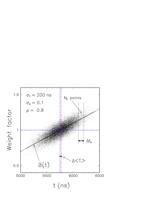
Figure 1: Toy scatter plot of the amplitudes versus the mean times of 15000 waveforms. The points have been extracted from a bivariate normal distribution with parameters indicated in the plot. The band delimited by the two vertical dotted lines indicates a generic time interval $\Delta t_{k}$ centered around $\bar{T}_{k}$, which contains $N_{k}$ points [see the discussion of Eq. (10)]. The dashed (dotted-dashed) vertical line indicates the average time obtained with the correct (incorrect) PDF-composing procedure. The difference between of the two averages is $\Delta\langle T_{i}\rangle\sim 18\,$ns. See the text for details.

In this case the correct normalization of the PDF is obtained by imposing the condition

$$\sum_{i=1}^{N}a_{i}=N\,,$$ (6)

equivalent to set equal to one the average value of the amplitudes ($\langle a_{i}\rangle=1$). The average time of the correct PDF is

$$\langle T_{i}\rangle=\frac{1}{N}\sum_{i=1}^{N}T_{i}\,,$$ (7)

while that obtained with the wrong PDF is

$$\langle T_{i}\rangle^{\prime}=\frac{1}{N}\sum_{i=1}^{N}a_{i}T_{i}\,,$$ (8)

the difference among the two estimates being

$$\Delta\langle T_{i}\rangle\equiv\langle T_{i}\rangle^{\prime}-\langle T_{i}\rangle=\frac{1}{N}\sum_{i=1}^{N}(a_{i}-1)T_{i}\,.$$ (9)

One can always time-order the $N$ times $T_{i}$’s and divide the time interval $[T_{1},T_{N}]$ in an integer number $K$ of subintervals $\Delta t_{k}$’s of equal-width $\Delta t$. In this way the time shift takes the approximate form

$$\Delta\langle T_{i}\rangle\simeq\frac{1}{N}\sum_{k=1}^{K}(\bar{a}_{k}-1)\bar{T}_{k}N_{k}\,,$$ (10)

where $N_{k}$ is the number of waveforms having mean time lying within the $k$-th subinterval positioned around their average time $\bar{T}_{k}$, and obeying the normalization condition

$$\sum_{k=1}^{K}N_{k}=N\,,$$ (11)

while $\bar{a}_{k}$ designates the average of their weight factors. The procedure outlined above can be better appreciated with the help of Fig. 1, which displays a toy scatter plot of 15000 points, each one representing a waveform with average time $T_{i}$ and amplitude $a_{i}$. In the limit $N\to\infty$ it makes sense to consider the limit $\Delta t\to 0$, which allows us to establish the following correspondences

$$N_{k}\to \frac{dN}{dt}dt\,,$$ (12)

$$\bar{a}_{k}\to \bar{a}(t)\,.$$ (13)

The density of points $dN/dt$ can be identified (apart from a proportionality factor) with the statistical distribution [call it $f(t)$] of the waveforms’ mean-time variable $t$, while $\bar{a}(t)$ represents the conditional expectation value of the amplitude variable $a$ at a given value of the variable $t$. In the continuos limit the discrete sums in Eq. (10) are replaced by integrals, thus obtaining for the time shift

$$\Delta\langle T\rangle\equiv\lim_{\Delta t\to 0}\Delta\langle T_{i}\rangle=\frac{\int{dt\,[\bar{a}(t)-1]\,t\,f(t)}}{\int dt\,f(t)}\,.$$ (14)

In order to proceed to the evaluation of the integrals in Eq. (14) we must make some (reasonable) assumptions on the form of the statistical distribution of the mean times $T_{i}$’s and of the associated amplitudes $a_{i}$’s. As a working hypothesis, it seems plausible to assume that their values are extracted from a bivariate normal distribution, characterized by the two standard deviations $\sigma_{T}$ and $\sigma_{A}$ and by the correlation coefficient $\rho$. In such a case, the following linear relation will hold

$$\bar{a}(t)=\langle a\rangle+\beta(t-\langle t\rangle)\,,$$ (15)

where $\langle t\rangle$ and $\langle a\rangle$ designate the averages of the two random variables and the coefficient $\beta$ is given by

$$\beta=\rho\frac{\sigma_{A}}{\sigma_{T}}\,.$$ (16)

Taking into account that the average amplitude [see Eq. (6)] is unitary by construction, Eq. (15) becomes

$$\bar{a}(t)=1+\rho\frac{\sigma_{A}}{\sigma_{T}}(t-\langle t\rangle)\,.$$ (17)

Such a linear relation is represented by the regression line shown in Fig. 1. The distribution $f(t)$ in Eq. (14) is by construction a gaussian distribution with standard deviation $\sigma_{T}$, being a marginal distribution of the native bivariate normal distribution. By substituting Eq. (17) in Eq. (14), and making use of elementary gaussian integrals, one finally arrives at the result

$$\Delta\langle T\rangle=\beta\,\sigma_{T}^{2}=\rho\,\sigma_{A}\,\sigma_{T}\,.$$ (18)

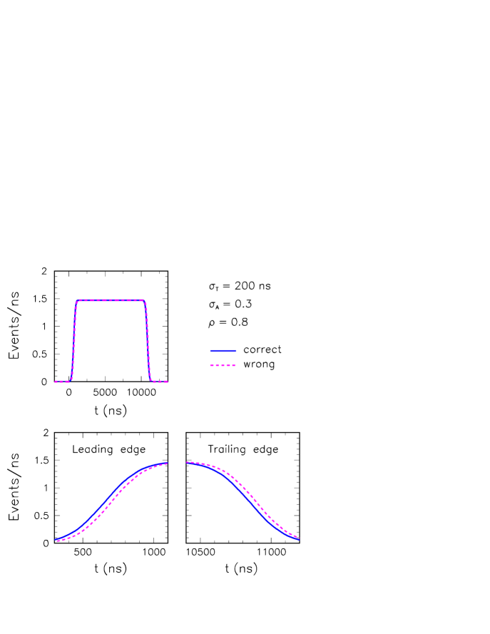
Figure 2: Effect of the incorrect procedure of PDF-composing. Both PDFs have been obtained summing up 15000 simulated rectangular waveforms having a fixed width of $10.2\,\mu$s. In one (correct) case the mean times are random numbers extracted from a gaussian distribution with standard deviation $\sigma_{T}$, while the weight factors are identical and unitary. In the other (wrong) case both the mean times and the weight factors are random numbers extracted from a bivariate normal distribution with standard deviations $\sigma_{T}$ and $\sigma_{A}$ and a correlation coefficient $\rho$. In the lower panels, representing a zoom of the edges of the two PDFs, a shift $\Delta\langle T_{i}\rangle\sim 48\,$ns of the average time can be appreciated. The dispersion of the amplitudes $\sigma_{A}$ has been taken three times bigger than its real estimated value for a better visual clarity.

Equation (18) makes explicit what could be grasped on an intuitive basis: In the presence of a non-zero correlation among the waveforms’ mean times and their intensities, the use of the wrong procedure of PDF-composing leads to a shift of the average time of the PDF. In particular, for a positive (negative) correlation coefficient the wrong method leads to an over(under)-estimation of the average neutrino emission time, and a consequent under(over)-estimation of its time of flight. Figure 2 illustrates such an effect on a toy PDF generated by combining $15000$ rectangular waveforms of equal width, and having mean times and intensities distributed according to a bivariate normal distribution. In this simple case, the shift of the average PDF time merely manifests itself as a shift of its edges.

Let us now try to quantify the three parameters entering Eq. (18): (I) A reliable estimate of the dispersion of the intensities can be deduced from the documentation publicly available on the CNGS website [4]. From Fig. 3 in [5] and the two figures shown at page 24 in [6]), we can infer $\sigma_{A}\sim 0.1$, at least for what concerns the 2009 and 2010 operational periods; (II) Without knowledge of the 15000 waveforms it is difficult to make a reliable estimate of their mean times’ dispersion $\sigma_{T}$. An upper bound for this parameter can be derived by observing that the width of the PDF is bigger than that of the individual waveforms as a result of the broadening effect induced by the summing procedure. From Fig. 14 in [1] a PDF width of about $11.2\,\mu$s can be estimated, about $700\,$ns bigger than the width of the single waveforms. Assuming that the whole PDF enlargement derives from the dispersion of the mean times of the composing waveforms, we derive $\sigma_{T}\sim 200\,$ns. The reliability of such an estimate is corroborated by the toy Monte Carlo simulations used to produce the PDFs in Fig. 2, whose edges look quite similar to those obtained in the real case (see Fig. 14 in [1]). Of course, part of the broadening effect may come from other factors such as a variable width of the waveforms. Therefore, such an estimate must be intended as an upper bound; (III) Concerning the correlation coefficient $\rho$, we observe that for each waveform $W_{i}$, the start-time of the digitation window is the trigger-time of the kicker magnet (see Fig. 3 and the related discussion on pages 5 and 12 in [1]). Such a time is set by the Wave Form Digitizer (WFD) as the common (arbitrary) time origin for each waveform before the summation procedure. This implies that shorter (longer) waveforms will have a smaller (bigger) mean time. In turn, the discussion made in [7] (see the comment on Fig. 2 at page 4), reveals that more (less) intense waveforms have systematically a longer (shorter) duration. Therefore, it seems quite natural to expect a positive correlation coefficient $\rho$, although no firm conclusion can be traced without having direct knowledge of the 15000 waveforms.

Inserting in Eq. (18) the estimated value of $\sigma_{A}$ and the upper bound for that of $\sigma_{T}$ we deduce that, for a positive correlation $\rho\sim 1$, a maximal shift of about $20\,$ns can be induced. Such an upper bound can be slightly altered as a consequence of the following two factors: (I) A non-gaussian behavior of the intensities’ and mean times’ distributions; (II) The potential effects (not considered in our toy simulations) of the wrong PDF-composing procedure on the shape of the flat-top of the PDF.

5 Relevance of the PDF-composing procedure to the future high precision short bunch measurements

Although we have discussed the case of long waveforms as those used in the first measurement by the OPERA collaboration, it is important to stress that our considerations are valid independently of the duration of the proton pulses used to inject the neutrinos. In particular, our main result provided in Eq. (18) remains valid for setups using very short bunches as those adopted by the OPERA collaboration for their second cross-check measurement and by ICARUS, and which (presumably) will be used by future high precision experiments.

One may be induced to think that the PDF approach is unnecessary when using very short pulses. However, this is not the case if one intends to obtain a precision on the neutrino time of flight comparable or smaller than the width of the bunches themselves, which are typically a few nanoseconds long. To this regard it is important to observe that in the case of OPERA and ICARUS the short-bunch measurements were performed with the sole purpose of (dis-)confirming the (quite large) shift of $\sim 60\,$ns found in the first OPERA measurement, which is much bigger than the width of the short bunches (3 ns). For such a specific purpose, it was sufficient to generate a histogram of the neutrino interaction times (like that presented in Fig. 18 of [1] or in Fig. 3 of [2] ) and check that it was statistically compatible or incompatible with the original shift of about $60\,$ns.

However, the situation would be completely different should one intend to use the short-bunch technique to measure time shifts (potentially) smaller than the bunch width itself. In this case, resorting to the PDF method appears to be inescapable, as it constitutes the only way to make a quantitative and precise comparison between the time distribution of the neutrino events and the detailed time structure of the emitted bunches. In such circumstances implementing the correct PDF-composing procedure will be essential.

6 A consistency test

In principle, a Monte Carlo test should allow the identification and the quantification of a problem in the procedure of PDF composing. However, we must note that this was not the case for the type of simulations performed by the OPERA collaboration. Indeed, according to the information reported in [1] (see page 19), and the more detailed documentation provided in the PhD thesis [3] (see page 132), it emerges that the correctness of the PDF has been assumed a priori. In fact, at page 19 of [1] one can read: “Starting from the experimental PDF, an ensemble of 100 data sets of OPERA neutrino interactions was simulated. Data were shifted in time by a constant quantity, hence faking a time of flight deviation”. This implies that the correctness of the PDF was assumed a priori and was not tested a posteriori.

This circumstance lead us to deem it useful to show how a consistency check may be performed in order to test the correctness PDF-composing procedure. In addition, we note that although we think we have clearly shown which of the two methods is the correct one at the theoretical level, the reader may find useful to have at his disposal also a numerical test of the issue in question. For such a test one has to reproduce a high number of virtual experiments as follows. In each of them one should: (I) Propagate at the speed of light the few-years-long train made of millions of waveforms so as to generate $N\sim O(10^{4})$ neutrino interactions in the detector with their own times; (II) Identify the associated $N$ waveforms; (III) Build a toy PDF using one of the two alternative methods we have discussed (first sum and then normalize and vice-versa) ; (IV) Compare such two PDF’s with the distribution of the neutrino interactions times so as to derive an a posteriori estimate of the neutrino velocity. By repeating such a simulation a sufficiently high number of times, the proposed test will tell the experimenters if the used PDF-composing method is correct or not. Indeed, when using the correct PDF-composing procedure, the estimate of the neutrino velocity obtained a posteriori will turn out to be statistically compatible with that imposed a priori (the velocity of light). When using the wrong procedure, two possibilities may occur: (A) The a posteriori estimate of the neutrino velocity is different from its value assumed a priori, thus indicating that the adopted method is wrong and making possible to quantify the error it has induced; (B) The a posteriori estimate is compatible with that used a priori, thus indicating that the use of the wrong method has harmless consequences: Although wrong at a conceptual level, it induces an error that is quantitatively irrelevant. This second circumstance is what would occur in the presence of a negligibly small value of one (or more) of the three parameters ($\rho$, $\sigma_{A}$, $\sigma_{T}$) entering Eq. (18).

7 Conclusions

We have discussed a conceptual issue concerning the statistical measurement of the neutrino velocity. We have evidenced that: (I) There are in principle two ways to obtain the global PDF from the single waveforms (first sum and then normalize or vice versa); (II) The second is the correct one at a conceptual level; (III) The use of the incorrect method can lead to a wrong inference of the neutrino time of flight, an effect for which we have provided an analytical description; (IV) The Monte Carlo tests performed by OPERA would have been unable to identify a problem in the procedure of combination of the waveforms; (V) We have proposed a consistency check able to detect such a kind of problems.

Note added

The original motivation of our paper was provided by the observation that the OPERA collaboration originally had reported an incorrect statistical procedure in the first version of [1]. Indeed, reading that first version, it emerged that the single waveforms had been first summed together and then their sum had been normalized to the total number of neutrino interactions observed in the detector (see page 14 of the first version of [1]). The more extensive information provided in the PhD thesis [3] (explicitly mentioned in [1]) corroborated that circumstance (see pages 124-125 of [3]).

After our preprint appeared, a second version of the OPERA paper [1] has been posted on arXiv. Differently from the first one, the second version reports the correct PDF-composing procedure. The opposite and correct order of the two operations of summing and normalization is now mentioned (see page 17 of the second version of [1]), although no comment has been included to explain the change made on such a delicate point. At present no further investigation on the issue in question is possible from outside the OPERA collaboration, as the relevant raw data (the time stamps of the 15000 neutrino interactions and those of the associated proton waveforms) have not been made publicly available.

References

- [1] T. Adam et al. [OPERA Collaboration], “Measurement of the neutrino velocity with the OPERA detector in the CNGS beam,” [arXiv:1109.4897 [hep-ex]] (versions 1 and 2).
- [2] M. Antonello et al. [ICARUS Collaboration], “Measurement of the neutrino velocity with the ICARUS detector at the CNGS beam,” arXiv:1203.3433 [hep-ex].
-
[3]
G. Brunetti,“Neutrino velocity measurement with the OPERA experiment in the CNGS beam”,
PhD thesis, in joint supervision of the Université Claude Bernard Lyon-I and Universitá di Bologna, 2011,
http://operaweb.lngs.infn.it:2080/Opera/phpmyedit/theses-pub.php - [4] http://proj-cngs.web.cern.ch/proj-cngs/
- [5] E. Gschwendtner et al.,“Performance and Operational Experience of the CNGS Facility”, contribution to IPAC10, First International Particle Accelerator Conference, Kyoto, Japan, 23-28 May 2010, CERN-ATS-2010-153. Available at [4].
- [6] E. Gschwendtner, “CNGS Operational Performance”, talk presented at the 7th International Workshop on Neutrino Beams and Instrumentation, J-PARC, Tokai, Japan, 28 - 31 August 2010. Transparencies available at [4].
- [7] E. Gaxiola, W. Hofle and E. Vogel, “Damping of betatron oscillations in the SPS appearing at the two step extraction of CNGS beam”, CERN-AB-2005-016-ABP. Available at [4].