Leptogenesis in the presence of
exact flavor symmetries

D. Aristizabal Sierra^a,, Federica Bazzocchi^b,

^aIFPA, Dep. AGO, Universite de Liege, Bat B5,
Sart Tilman B-4000 Liege 1, Belgium.

^bSISSA and INFN, Sezione di Trieste,
Via Bonomea 265, 34136 Trieste, Italy.

In models with flavor symmetries in the leptonic sector leptogenesis can take place in a very different way compared to the standard leptogenesis scenario. We study the generation of a $B-L$ asymmetry in these kind of models in the flavor symmetric phase pointing out that successful leptogenesis requires (i) the right-handed neutrinos to lie in different irreducible representations of the flavor group; (ii) the flavons to be lighter at least that one of the right-handed neutrino representations. When these conditions are satisfied leptogenesis proceeds due to new contributions to the CP violating asymmetry and—depending on the specific model—in several stages. We demonstrate the validity of these arguments by studying in detail the generation of the $B-L$ asymmetry in a scenario of a concrete $A_{4}$ flavor model realization.

1 Motivation

Observational data from the abundances of light elements (D, ³He, ⁴He and Li) in addition to precision observations of the cosmic microwave background (CMB) temperature fluctuations allow the determination of the cosmic baryon asymmetry, $Y_{\Delta_{B}}=(n_{B}-n_{\bar{B}})/s=(8.75\pm 0.23)\times 10^{-11}$ (with $n_{B}$ ($n_{\bar{B}}$) the baryon (antibaryon) number density and $s$ the entropy density) [1]. Though the conditions for dynamically generating this quantity are well known and established [2] the cosmic baryon asymmetry poses a puzzle in particle physics: the standard model (SM) fails to explain such a large asymmetry, thus implying the presence of new physics accounting for $Y_{\Delta_{B}}$.

Leptogenesis is a scenario in which a lepton asymmetry $Y_{\Delta_{L}}$ is generated in the lepton sector and partially reprocessed into $Y_{\Delta_{B}}$ by SM electroweak sphaleron processes (for a comprehensive review see [3]). The generation of $Y_{\Delta_{L}}$ requires, in addition to CP violation and departure from thermodynamical equilibrium, lepton number breaking. Accordingly, in these class of scenarios two in principle unrelated puzzles are linked, the origin of neutrino masses and the baryon asymmetry. Among all the possible neutrino mass models present in the literature the standard seesaw (type I seesaw) [4] provides the framework for standard leptogenesis, in which the lepton asymmetry proceeds via the out-of-equilibrium and CP violating decays of the lightest right-handed (RH) electroweak singlet neutrino.

Most of the studies of leptogenesis are based on the assumption that there is no new physics between the lepton number breaking scale and the electroweak scale that can sizable affect the way in which leptogenesis takes place. Though some analysis in scenarios including flavor symmetries above the electroweak scale have been done, and have proved that the presence of new energy scales and new degress of freedom may have an impact on the way leptogenesis proceeds [5, 6, 7, 8], all of them are based on the same assumption, namely the lepton number breaking scale is below the scale at which the flavor symmetry is broken .

The idea to ascribe to a flavor symmetry to explain particle masses and mixings dates backs to the late 1970’s [11]. Originally flavor symmetries were introduced to explain quark structures and only after neutrino oscillation data the use of horizontal symmetries in the lepton sector has become more challenging and interesting. In particular, in the last years it has been shown that lepton mixing may be well described by discrete non Abelian symmetries (see [12] and references therein for further details). Given that in these kind of models both, the lepton number and flavor breaking scales are free parameters the question about how does leptogenesis proceeds in the flavor symmetric phase proves to be quite reasonable.

In more detail, let us suppose to have a non Abelian flavor symmetry group $G_{F}$ under which the RH neutrinos and left-handed SM leptons have definitive transformations. We introduce a cutoff scale $\Lambda$ since we will deal with non-renomalizable operators. The scenario which we are interested in is the following: the lepton number breaking scale, characterised by the RH neutrino mass, $M_{N}$, is larger than the scale at which $G_{F}$ is broken, $v_{F}$. This means that the Yukawa mass matrices above and below $v_{F}$ are different: in particular the Yukawa Dirac matrix below $v_{F}$ is proportional to the Dirac mass matrix—the proportionality factor represented by the SM Higgs vacuum expectation value (vev). Flavon masses, $M_{\phi}$, are taken as free parameters, clearly not too far from $v_{F}$ but above it. Clearly it holds $\Lambda>M_{N},M_{\phi}>v_{F}$.

Our discussion is based on the class of symmetries that explain neutrino masses and lepton mixings and may be be generalized to any flavor symmetry, Abelian or not, discrete or continuos. We will exemplify our arguments by doing a full analysis of the generation of the $B-L$ in a concrete model that at low scale exhibits exact TriBiMaximal (TBM) mixing at leading order. The reason for this choice is very simple: it has been shown that when exact TBM mixing is induced by type I seesaw the CP violating asymmetry is zero and acquires a non-vanishing value only when lepton mixing deviates from TBM [13, 14, 7]. In type II seesaw models this could be also the case if only two electroweak triplets are present and they both are family singlets [16]. Extended models featuring interplay between type I and II seesaws have been also analysed and the conclusion is that in these cases it is also possible to identify a generic class of minimal models in which the CP asymmetry vanishes as well [15].

The most recent analysis indicates that TBM is not anymore in perfect agreement with neutrino experimental data since the reactor angle predicted by TBM is zero, while this value is now excluded at $3\sigma$ level [17]. However TBM remains a good approximation for the lepton mixing matrix and we will consider a model that predicts exact TBM for its simplicity in showing the feasibility of leptogenesis in the regime $\Lambda>M_{N},M_{\phi}>v_{F}$.

The paper is organized in the following way: next section is general and we enumerate the general conditions necessary to obtain a CP asymmetry, $\epsilon_{N}$, in the flavor symmetric regimen. Section 3 shows how the proposed conditions work by mean of a complete analysis of a specific model based on the flavor symmetry $A_{4}$. The model main features and neutrino phenomenology are briefly discussed and the generation of the $B-L$ asymmetry is explained in detail. Section 4 is devoted to our conclusions. The calculation of the reaction densities necessary for the analysis of the washout processes studied in sec. 3 are given in appendix A.

2 Leptogenesis in the flavor symmetric phase

We have already anticipated in the introduction that in models for leptonic flavor mixing four energy scales can be distinguished, namely a cutoff scale $\Lambda$—or in general a scale of heavy matter—, the lepton number breaking scale—determined by the RH neutrino masses—$M_{N}$, the flavons scale $M_{\phi}$—determined by the masses of the scalars that trigger the flavor symmetry breaking—and the scale at which the flavor symmetry is broken, $v_{F}$. Though $\Lambda>M_{N},M_{\phi},v_{F}$ the scales $M_{N}$, $M_{\phi}$ and $v_{F}$, being free parameters, can follow any hierarchy. Since we are concerned about leptogenesis in the flavor symmetric phase it is clear $v_{F}<M_{N},M_{\phi}$. This constraint in turn has an implication: if the flavor symmetry enforces the RH neutrinos to belong to the same $G_{F}$ irreducible representation, $R$, leptogenesis will not be achievable: in the flavor symmetric phase the RH neutrinos have a common universal mass and therefore the CP violating asymmetry $\epsilon_{N}$ vanishes [18].

As a consequence, in these kind of models viable leptogenesis requires RH neutrinos to belong to different $G_{F}$ irreducible representations $R_{i}$, so a mass splitting among the masses of the different representations can be accomodated. Let us assume the existence of $k$ electroweak lepton doublets placed in $r$ representations $L_{r}$, $m$ RH neutrinos lying in $p$ representations $N_{p}$ and $n$ electroweak singlet scalars arranged in $q$ representations $S_{q}$. Assuming the SM Higgs $SU(2)$ doublet, $H$, to be a $G_{F}$ singlet the $i$-th RH neutrino representation can only decay to final states containing $L_{i}$. Accordingly, three type of models can be distinguished:

1. For any RH neutrino representation $N_{i}\sim R_{i}$ there is a lepton doublet representation $\bar{L}_{i}\sim R^{\prime}_{i}$ with which a gauge flavor invariant renormalizable operator $\bar{L}_{i}\,N_{i}\,H$ can be built .

2. Only for a set of the RH neutrino representations a gauge flavor invariant renormalizable operator $\bar{L}_{i}\,N_{i}\,H$ exist

3. For non of the RH neutrino representations the operator $\bar{L}_{i}\,N_{i}\,H$ can be built.

In cases 1 and 2 the standard one-loop vertex and wave-function corrections to the tree-level decay exist however the CP violating asymmetry derived from their interferences and the corresponding tree-level process vanishes. The proof of this statement is easy. Suppose $N_{i}$ transforms as the $R_{i}$ representation of $G_{F}$. To recover the correct kinetic term we know $R_{i}^{*}R_{i}=\delta_{\alpha_{i}\beta_{i}}$ should hold (here $\alpha_{i},\beta_{i}$ are the indices of the $R_{i}$ representation). The same applies for $\bar{L}_{i}\sim R^{\prime}_{i}$. Now, the standard contribution to the CP asymmetry involves the imaginary part of the off-diagonal elements of the matrix $Y\,Y^{\dagger}$, where $Y$ is a generic Yukawa coupling matrix defined in the stage of unbroken flavor symmetry. This Yukawa coupling matrix is given by the Clebsch-Gordan coefficients arising from the contractions $R^{\prime}_{i}\,R_{i}$, thus implying that the matrix $Y\,Y^{\dagger}$ is determined in turn by the contractions $R^{\prime}_{i}\,R_{i}\,R_{i}^{*}\,{R^{\prime}}_{i}^{*}$, which demonstrates that $YY^{\dagger}$ is diagonal. Viable leptogenesis is, therefore, possible only if new contributions ($\epsilon_{N}^{\text{New}}$) to $\epsilon_{N}$ are present, and this is possible only if at least for one of the RH neutrino representations the condition $M_{N}>M_{\phi}$ is satisfied

In case 3 it is possible that $N_{i}$ may have $n>2$ body decays by means of non renormalizable operators. In this scenario one should modify the standard case in order to include $n$-body decays. However, due to space suppression factors the CP asymmetry generated is expected to be small. For this reason in what follows we do not consider this case.

Assuming the flavons are lepton conserving states no $B-L$ asymmetry can be generated via $\phi$ decays. However, once the condition $M_{N}>M_{\phi}$ is satisfied they can play an essential role in the generation of the $B-L$ asymmetry, not only because they lead to novel contributions to $\epsilon_{N}$, but because in some cases they can even allow some RH neutrino representations to have new decay modes that can change the way in which leptogenesis takes place. Once the conditions discussed above are satisfied not much more, from a general perspective, can be said and the way in which the $B-L$ asymmetry is generated depends upon the particular flavor model. Hereafter are discussion will rely on a particular $A_{4}$ flavor model realization.

3 Setup

We consider the non-supersymmetric version of a model inspired by the Altarelli-Feruglio model discussed in [19] of which the type-I seesaw formulation has been analyzed in [20]. In the original model supersymmetry is introduced to induce the correct spontaneous breaking of the flavor symmetry. Here we assume that by adding additional discrete Abelian symmetries or ad hoc soft terms the scalar potential may be arranged in such a way that the desired breaking is realized. At this level the model presented is still a toy model, however our findings will hold even in its supersymmetric version.

3.1 The $\boldsymbol{A_{4}}$ group

Before entering into the details of the model, for completeness, we will briefly discuss the basic ingredients of the $A_{4}$ discrete group in which the model presented here is based. $A_{4}$ is the group of even permutations of 4 objects. It has 4 irreducible representations: one triplet and three singlets $1,1^{\prime},1^{\prime\prime}$. $A_{4}$ may be thought as generated by two elements $S,T$ satisfying

$$S^{2}=T^{3}=(ST)^{3}=1\,.$$ (1)

In what follows we will work in the $A_{4}$ basis in which the triplet representation of $T$ is diagonal, namely

$$S=\frac{1}{3}\left(\begin{array}[]{ccc}-1&2&2\\ 2&-1&2\\ 2&2&-1\end{array}\right)\,, T=\left(\begin{array}[]{ccc}1&0&0\\ 0&\omega&0\\ 0&0&\omega^{2}\end{array}\right)$$ (8)

with $\omega^{3}=1$. The multiplication rules in this basis are given by

$$(ab)_{1}=(a_{1}b_{1}+a_{2}b_{3}+a_{3}b_{2})\,,$$

$$(ab)_{1^{\prime}}=(a_{3}b_{3}+a_{1}b_{2}+a_{2}b_{1})\,,$$

$$(ab)_{1^{\prime\prime}}=(a_{2}b_{2}+a_{1}b_{3}+a_{3}b_{1})\,,$$

$$(ab)_{3_{s}}=(2a_{1}b_{1}-a_{2}b_{3}-a_{3}b_{2},2a_{3}b_{3}-a_{2}b_{1}-a_{1}b_{2},2a_{2}b_{2}-a_{3}b_{1}-a_{1}b_{3})\,,$$

$$(ab)_{3_{a}}=(a_{2}b_{3}-a_{3}b_{2},a_{1}b_{2}-a_{2}b_{1},a_{3}b_{1}-a_{1}b_{3})\,,$$

where $a$ and $b$ are triplets of $A_{4}$, namely $a\sim(a_{1},a_{2},a_{3}),b\sim(b_{1},b_{2},b_{3})$ and for the singlet representations the multiplication rules are trivial

$$1^{\prime}\otimes 1^{\prime\prime}=1\,,\quad 1^{\prime}\otimes 1=1^{\prime}\,,\quad 1^{\prime\prime}\otimes 1=1^{\prime\prime}\,.$$ (10)

3.2 The model

In our model four RH neutrinos are added to the SM field content. Three of them, $\nu_{T}$, form an $A_{4}$ triplet while the fourth, $\nu_{4}$, is an $A_{4}$ singlet. The SM lepton doublets, $l_{1},l_{2},l_{3}$, transform as an $A_{4}$ triplet. For simplicity we assign flavor charges using the Weyl spinor notation. The RH 4-dim Majorana fermion will be therefore defined as

$$N=\left(\begin{array}[]{c}(\nu_{R})^{C}\\ \nu_{R}\end{array}\right)\,.$$ (11)

It is important to notice that if $l\sim(l_{1},l_{2},l_{3})$ transforms as a triplet the requirement of recovering the correct kinetic term according to the group multiplication rules imposes that ${l}^{\dagger}$ transforms as a triplet but ordered as ${l}^{\dagger}\sim({l}^{\dagger}_{1},{l}^{\dagger}_{3},{l}^{\dagger}_{2})$. On the contrary we order $\nu_{T}^{\dagger}$ as $(\nu^{\dagger}_{1},\nu^{\dagger}_{2},\nu^{\dagger}_{3})$ thus $\nu_{T}\sim(\nu_{1},\nu_{3},\nu_{2})$.

RH charged leptons transform as the 3 one dimensional representation of $A_{4}$, namely $1,1^{\prime},1^{\prime\prime}$. Two $A_{4}$ scalar triplets, $\phi_{T}$ and $\phi_{S}$, our flavons, are added. Once the flavor symmetry is broken they will give rise to the correct mass matrices.

3.2.1 Neutrino mass matrices

Given the field content previously described the Lagrangian for the lepton sector—not including the kinetic terms—reads as

$$-\mathcal{L} = \frac{M_{\nu T}}{2}(\nu_{TR}^{{\dagger}}\nu^{c}_{TR}+\nu_{TR}^{c{\dagger}}\nu_{TR})_{1}+\frac{M_{\nu 4}}{2}(\nu_{4R}^{c{\dagger}}\nu_{4R}+\nu_{4R}^{\dagger}\nu_{4R}^{c})_{1}$$ (12)

$$+ \lambda[\nu_{TR}^{{\dagger}}\nu^{c}_{TR}\phi_{S}]_{1}+\lambda^{*}[\nu_{TR}^{c{\dagger}}\nu_{TR}\phi^{*}_{S}]_{1}$$

$$+ \xi[\nu_{TR}^{{\dagger}}\phi_{S}]_{1}\nu^{c}_{4R}+\xi^{*}\nu_{4R}^{c{\dagger}}[\nu_{TR}\phi^{*}_{S}]_{1}$$

$$+ y_{1}\epsilon_{\alpha\beta}(\nu_{TR}^{\dagger}l_{L}^{\alpha})_{1}H^{\beta}+y^{*}_{1}\epsilon_{\alpha\beta}(l_{L}^{{\dagger}\alpha}\nu_{TR})_{1}H^{\beta}$$

$$+ y_{2}\frac{1}{\Lambda}\epsilon_{\alpha\beta}[\nu_{TR}^{\dagger}l_{L}^{\alpha}\phi_{S}]_{1}H^{\beta}+y_{2}^{*}\frac{1}{\Lambda}\epsilon_{\alpha\beta}[l_{L}^{{\dagger}\alpha}\nu_{TR}\phi^{*}_{S}]_{1}H^{*\beta}$$

$$+ y_{3}\frac{1}{\Lambda}\epsilon_{\alpha\beta}\nu_{4R}^{\dagger}[l_{L}^{\alpha}\phi_{S}]_{1}H^{\beta}+y_{3}^{*}\frac{1}{\Lambda}\epsilon_{\alpha\beta}[l_{L}^{{\dagger}\alpha}\phi^{*}_{S}]_{1}\nu_{4R}H^{\beta}$$

$$+ y_{e}^{i}\frac{1}{\Lambda}e^{c}_{Ri}[\phi_{T}l_{L}^{\alpha}]_{i}\tilde{H}^{\alpha}+\text{H.c.}\,.$$

We have assumed the presence of an Abelian $Z_{N}$ with $N>2$ that forbids $\phi_{S,T}$ and $\phi_{S,T}^{*}$ to have the same couplings and we are assuming the flavons to be complex fields. Note that in this class of models this kind of Abelian symmetries are always present to prevent interferences between $\phi_{T}$ and $\phi_{S}$.

Note also that we can rephase the RH neutrinos to make $M_{\nu T}$ and $M_{\nu 4}$ real. After doing so we still have the freedom to rephase the lepton $A_{4}$ triplet and the flavon $A_{4}$ singlet, absorbing in that way other two CP phases. These basis rotations allow us to choose $\lambda$ and $y_{3}$ to be real.

In eq. (12) the last row describes charged leptons: $i$ stays for $1,1^{\prime},1^{\prime\prime}$ and the $[...]_{i}$ stays for the triplet contractions in the one dimensional representations. In the other rows $[...]_{1}$ stays for 2 or 3 triplets contracted in a singlet. Greek indices $\alpha$ and $\beta$ label $SU(2)_{L}$ degrees of freedom, $H$ the SM Higgs doublet, and as usual $\tilde{H}=i\sigma_{2}H$. We assume that the additional $Z_{N}$ symmetry forbids the coupling of $\phi_{T}$ and $\phi_{S}$ to neutrinos and charged leptons respectively. The $A_{4}$ basis chosen is useful because when $\phi_{T}$ develops a vev according to $\left\langle\phi_{T}\right\rangle\sim v_{T}(1,0,0)$ the charged lepton Yukawa mass matrix is diagonal. On the other hand when $\phi_{S}$ acquires the vev $\left\langle\phi_{S}\right\rangle\sim v_{S}(1,1,1)$ the Dirac Yukawa matrix, $Y_{\nu}$, and the RH neutrino mass matrix, $\mathcal{M}_{N}$ are diagonalized by the so-called TBM mixing matrix. Thus after electroweak symmetry breaking the light neutrino mass matrix,

$$m_{\nu}\sim-m_{D}^{T}\cdot\mathcal{M}_{N}^{-1}\cdot m_{D}$$ (13)

is diagonalized by the TBM mixing matrix as well. Clearly $m_{D}=Y_{\nu}v_{H}$, with $\left\langle H\right\rangle=v_{H}$.

Both $\mathcal{M}_{N}$ and $Y_{\nu}$ get a contribution above ($>$) and below ($<$) the scale $v_{F}\sim v_{T}\sim v_{S}$, so we may write

$$\mathcal{M}_{N} = \mathcal{M}^{>}_{N}+\mathcal{M}^{<}_{N}\,,$$

$$Y_{\nu} = Y_{\nu}^{>}+Y_{\nu}^{<}\,,$$ (14)

with

$$\mathcal{M}^{>}_{N} \sim \left(\begin{array}[]{cccc}A&0&0&0\\ 0&0&A&0\\ 0&A&0&0\\ 0&0&0&D\end{array}\right)\,,\quad Y_{\nu}^{>}\sim\left(\begin{array}[]{ccc}a&0&0\\ 0&0&a\\ 0&a&0\\ 0&0&0\end{array}\right)$$ (23)

$$\mathcal{M}^{<}_{N} \sim \left(\begin{array}[]{cccc}2B&-B&-B&C\\ -B&2B&-B&C\\ -B&-B&2B&C\\ C&C&C&0\end{array}\right)\,,\quad Y_{\nu}^{<}\sim\left(\begin{array}[]{ccc}2b&-b&-b\\ -b&2b&-b\\ -b&-b&2b\\ c&c&c\end{array}\right)\,.$$ (32)

with $A\sim M_{\nu T},B\sim\lambda v_{S},C\sim\xi v_{S}$, $D\sim M_{\nu 4}$ and $a\sim y_{1},b\sim y_{2}v_{S}/\Lambda,c\sim y_{3}v_{S}/\Lambda$ for the RH neutrino and Yukawa Dirac mass matrix respectively. Without loss of generality $v_{S}$ may be taken real.

Defining $\epsilon_{S}=v_{S}/\Lambda$, clearly in the limit $\epsilon_{S}\to 0$ the symmetry is restored and the light neutrinos are degenerate. Thus we expect in the majority of the cases a quasi-degenerate (QD) neutrino mass spectrum in which $|y_{1}|^{2}/M_{\nu T}$ controls the absolute mass scale while $y_{2},\lambda,\epsilon_{S}=v_{S}/\Lambda$ parametrize the neutrino atmospheric mass splitting. We may find an approximate analytical solution for the spectrum expanding in $\epsilon_{S}$. We have

$$m_{0} \sim |y_{1}|^{2}\frac{v_{H}^{2}}{M_{\nu T}}\,,$$

$$\frac{\Delta m^{2}_{sol}}{\Delta m^{2}_{atm}} \sim \frac{1}{2}+\frac{\epsilon_{S}}{2}(\epsilon_{X}+\epsilon_{X}^{2})\frac{(|y_{1}|^{2}\xi^{2}-2|y_{1}|y_{3}\xi\cos\phi_{y_{1}}+y_{3}^{2}\cos 2\phi_{y_{1}})}{|y_{1}|(|y_{1}|\lambda-2|y_{2}|\cos\Delta{\phi_{12}})}\,,$$ (33)

with $\epsilon_{X}=(M_{\nu T}-M_{\nu 4})/M_{\nu T}$, $\phi_{y_{1,2}}=\text{Arg}(y_{1,2})$ and $\Delta{\phi_{12}}=\phi_{y_{1}}-\phi_{y_{2}}$.

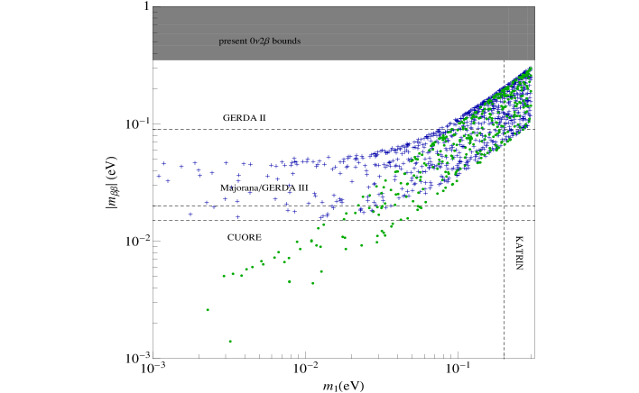
Figure 1: The predictions for $|m_{\beta\beta}|$ as a function of the lightest neutrino mass. The natural spectrum predicted by the model is QD, with both normal ordering (NO) and inverse ordering (IO) as indicated by the analytical approximations. Both QD-NO (QD-IO) and NH (IH) spectrum are indicated with green points (blue crosses). See the text for more details.

Equation (3.2.1) holds only in the regime $\epsilon_{S}<\epsilon_{X}$. When $\epsilon_{X}<\epsilon_{S}$ the analytical expressions become more cumbersome because the QD scenario is broken and both, the normal hierarchical (NH) and inverse hierarchical (IH) neutrino mass spectra become possible. The spectrum predicted by our model is shown in fig.1 by means of $m_{\beta\beta}$, the parameter relevant for neutrinoless double beta decay defined as $m_{\beta\beta}=[U_{\text{TBM}}\,\text{diag}(m_{1},\,m_{2},\,m_{3})\,U_{\text{TBM}}^{T}]_{11}$. It has been obtained by numerically diagonalizing the neutrino mass matrix below the scale $v_{S}$, fixing the neutrino mixing angles according to the TBM scheme and requiring the solar and atmospheric mass splittings to lie within their currents $3\,\sigma$ ranges [17]. The parameters entering in the mass matrix were varied according to: $[10^{-3},10^{-1}]$ for the dimensionless parameters, $\epsilon_{S}$ constrained to be below $10^{-1}$ and RH neutrino masses in the range $[10^{7},10^{14}]$ GeV. For all the points $\Lambda$ was taken to be larger than the heaviest RH neutrino mass. For completeness in the figure we have shown the future experimental bounds on $|m_{\beta\beta}|$ and $m_{1}$.

For what concerns the flavon sector the $Z_{N}$ symmetries allows only the mass term

$$M_{\phi}^{2}(\phi_{S}\phi_{S}^{*})_{1}\,.$$ (34)

Recalling now that $\phi^{*}_{S}\sim(\phi^{*}_{S1},\phi^{*}_{S3},\phi^{*}_{S2})$ we have that the flavon mass matrix is diagonal and CP even and odd states are degenerate.

3.2.2 Flavon Interaction Matrices

Above $v_{F}$ instead of $\mathcal{M}^{<}_{N},Y_{\nu}^{<}$ we have flavon-neutrino and flavon-Higgs-neutrino interaction matrices $\mathcal{I}_{N,\nu}$. Starting from the interactions

$$-\mathcal{L}_{I} = \frac{1}{2}\lambda[\nu_{TR}^{{\dagger}}\nu_{TR}^{c}\phi_{S}]_{1}+\frac{1}{2}\lambda^{*}[\nu_{TR}^{c{\dagger}}\nu_{TR}\phi^{*}_{S}]_{1}+\xi[\nu_{TR}^{{\dagger}}\phi_{S}]_{1}\nu^{c}_{4R}+\xi^{*}\nu_{4R}^{c{\dagger}}[\nu_{TR}\phi^{*}_{S}]_{1}$$ (35)

$$+ \frac{1}{\Lambda}y_{2}\epsilon_{\alpha\beta}[\nu_{TR}^{\dagger}l_{L}^{\alpha}\phi_{S}]_{1}H^{\beta}+\frac{1}{\Lambda}y_{2}^{*}\epsilon_{\alpha\beta}[l_{L}^{{\dagger}\alpha}\nu_{TR}\phi^{*}_{S}]_{1}H^{*\beta}\,,$$

we may write them using the 4-component spinors $N$ and $P_{L}l=l_{L}$ as

$$\frac{1}{2}\mathcal{I}^{k}_{N_{R}}(\phi^{*}_{S_{k}})_{ij}\bar{N}_{i}P_{R}N_{j}+\frac{1}{2}\mathcal{I}^{k}_{N_{L}}(\phi_{S_{k}})_{ij}\bar{N}_{i}P_{L}N_{j}$$ (36)

$$+\mathcal{I}_{D_{L}}^{k}(\phi_{S_{k}})_{ij}\epsilon_{\alpha\beta}\bar{N}_{i}P_{L}l^{\alpha}_{j}H^{\beta}+\mathcal{I}_{D_{R}}^{k}(\phi_{S_{k}}^{*})_{ij}\epsilon_{\alpha\beta}\bar{l}^{\alpha}_{i}P_{R}N_{j}\tilde{H}^{\beta}\,,$$

where $\mathcal{I}^{k}_{N_{L}}=\mathcal{I}^{k{\dagger}}_{N_{R}},\mathcal{I}_{D_{R}}^{k}=\mathcal{I}_{D_{L}}^{k{\dagger}}$ and $k$ labels the $\phi_{S},\phi_{S}^{*}$ flavons. Notice that in eq. (36) and for the rest of the paper we will indicate with $N_{i}$ the four RH neutrinos of the model under study, while in sec. 2 $N_{i}$ was referred to the group representations.

First of all we change basis going in the basis in which $\mathcal{M}^{>}_{N}$ is diagonal. Thus we have

$$\hat{\mathcal{M}}^{>}_{N} = U_{R}^{T}\cdot\mathcal{M}^{>}_{N}\cdot U_{R}=\mbox{Diag}(M_{\nu T},M_{\nu T},M_{\nu T},M_{\nu 4})=\mbox{Diag}\,(M_{{N_{i}}_{(i=1,2,3)}},M_{N_{4}})\,,$$

$$U_{R} = \frac{1}{\sqrt{2}}\left(\begin{array}[]{cccc}\sqrt{2}&0&0&0\\ 0&1&-i&0\\ 0&1&i&0\\ 0&0&0&\sqrt{2}\end{array}\right)\,,$$ (41)

$$\hat{Y}^{>}_{D} = U_{R}^{\dagger}\cdot Y^{>}_{D}=\frac{y_{1}}{2\sqrt{2}}\left(\begin{array}[]{ccc}\sqrt{2}&0&0\\ 0&1&1\\ 0&-i&i\\ 0&0&0\end{array}\right)\,.$$ (46)

It proves useful to write the interaction matrices as

$$\mathcal{I}^{k}_{N_{R}}(\phi^{*}_{S_{k}})_{ij}=({\mathcal{I}}^{>}_{N_{R}})^{k}_{ij}\,{\phi}_{k}\,,$$

$$\mathcal{I}_{D_{R}}^{k}(\phi_{S_{k}}^{*})_{ij}={(\mathcal{I}}^{>}_{D_{R}})^{k}_{ij}\,{\phi}_{k}$$ (47)

and similarly for $\mathcal{I}^{k}_{N_{L}}(\phi_{S_{k}})_{ij},\mathcal{I}_{D_{L}}^{k}(\phi_{S_{k}})_{ij}$. The ${\mathcal{I}}_{D_{R}}^{k}$ are $3\times 4$ matrices, being 4 the total number of RH neutrinos. Equation (3.2.2) may appear as redundant since in our model $\phi_{S}$ couples always linearly. However the advantage of our notation is that it holds even when operators of dimension higher than 5 are included.

3.3 CP asymmetries

In the standard leptogenesis scenario the lightest RH neutrino CP asymmetry, $\epsilon_{N}$, arises from the interference between the tree-level decay Feynman diagram and the one-loop vertex and wave function corrections [21]. Since $N_{4}$ does not have renormalizable couplings to the lepton doublets such diagrams do not exist in the case under consideration, regardless of the RH neutrino mass spectrum. New contributions due to the presence of the flavons degrees of freedom exist and depend upon the RH neutrino spectrum:

1. The $\boldsymbol{M_{N_{i}}>M_{N_{4}}}$ case: $N_{i}$ has standard $L_{i}H$ tree-level decays and, given the interactions in the Lagrangian (12), the only possible correction to this process arise from the one-loop correction to the effective vertex $N_{i}\phi_{i}L_{i}H$, as shown in fig. 2. Thus, the CP asymmetry in this case is obtained from the interference between diagrams 2(a) and 2(b).

2. The $\boldsymbol{M_{N_{4}}>M_{N_{i}}}$ case: Since $N_{4}$ couples to $N_{i}\phi_{i}$ at the renormalizable level a CP asymmetry for the two body decay process $N_{4}\to N_{i}\phi_{i}$ can be calculated from the interference between the corresponding tree-level diagram and the two-loop level diagram involving both effective couplings $N_{4}L_{i}\phi_{i}H$ and $N_{i}L_{i}\phi_{i}H$ (since $N_{4}$ does not couples to lepton doublets at the renormalizable level the one-loop correction to the process $N_{4}\to N_{i}\phi_{i}$ does not exist). There is another option involving $N_{4}$ three-body decays induced by the effective coupling $N_{4}L_{i}\phi_{i}H$. In this scenario a one-loop correction to the effective process does not exist either and the calculation of the CP asymmetry relies again on the two-loop level correction of the previous case.

Figure 2: Tree-level and one-loop correction diagrams accounting for $\epsilon_{N_{i}}$.

In case 1 the CP asymmetry arises in a different way compared to the standard case but in what regards the generation of the $B-L$ asymmetry there is no difference. In contrast, the cases in 2 are quite different: for the three-body decay scenario the differences are obvious, for the other scenario leptogenesis will take place in two stages, a first stage in which an asymmetry in $N_{i}$ is generated via the decays $N_{4}\to N_{i}\phi_{i}$ and a second stage in which the asymmetry in $N_{i}$ is partially transfered to the lepton doublets via $N_{i}$ decays and scatterings (a scenario of this kind has been discussed in [9, 22]). Note that in this case the CP asymmetry, being a two-loop order effect, would most likely yield a very tiny $B-L$ asymmetry. All these scenarios however exhibit a common feature, the generation of a $B-L$ asymmetry takes place in the flavor symmetric phase. So from now on we will focus on case 1, that as was already pointed out resembles standard leptogenesis.

The CP asymmetry in the decay of $N_{i}$ is defined according to

$$\epsilon_{N_{i}}=\sum_{k=e,\mu,\tau}\epsilon_{N_{i}}^{L_{k}}=\sum_{k=e,\mu,\tau}\frac{\Gamma_{N_{i}}^{k}-\bar{\Gamma}_{N_{i}}^{k}}{\Gamma_{N_{i}}^{k}+\bar{\Gamma}_{N_{i}}^{k}}\,,$$ (48)

where $\Gamma_{N_{i}}^{L_{k}}$ ($\bar{\Gamma}_{N_{i}}^{L_{k}}$) denotes the $N_{i}$ partial decay width for final states of flavor $k$ and carrying $+1$ ($-1$) unit of lepton number, and $\epsilon_{N_{i}}^{L_{k}}$ are the flavored CP asymmetries. However, here we are working in the context of an exact flavor symmetry. Since flavor is unbroken only flavor conserving processes may happen, that in our framework means $k=i$. Moreover flavor invariance and the representation used for our right and left-handed neutrinos imply that the three RH neutrinos produce the same amount of CP asymmetry and have exactly the same dynamics. Due to the complex nature of the scalar field components $\phi_{i}$ running in the loop 2(b) there is only one possible one-loop diagram of that type (contrary to the standard leptogenesis case for the wave-function correction), so the interference between the tree and one-loop level amplitudes (${\cal M}_{0}$ and ${\cal M}_{1}$) involves only one term. For two-body decays this interference is phase-space independent and consequently the calculation of $\epsilon_{N_{i}}$ can be simply done in terms of the products of ${\cal M}_{0}$ and ${\cal M}_{1}$ and approximating the denominator of (48) with $|{\cal M}_{0}|^{2}$ [9]. In the limit $M_{N_{i}}>>M_{N_{4}},M_{\phi}$ the CP asymmetry can be written as

$$\epsilon_{N_{i}}^{\ell_{i}}=-\frac{1}{8\pi}\frac{1}{|Y^{>}Y^{>\dagger}|^{2}_{ii}}\frac{M_{N_{i}}}{\Lambda}\mathfrak{I}\mbox{m}\left[(Y^{>}\,\mathcal{I}^{k}_{D_{R}})_{i4}\right]\,.$$ (49)

In the general case, without assuming any large hierarchy among the heaviest RH neutrino representation, the lightest one and the flavons, the expression for $\epsilon_{N_{i}}$ is far more involved. Fig. 3, obtained from the exact expression, shows the possible values of the CP asymmetry as a function of the effective cut-off scale $\Lambda$.

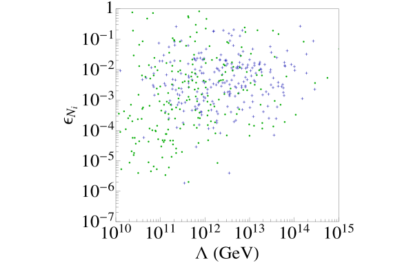
Figure 3: $\epsilon_{N_{i}}$ as a function of the cutoff scale $\Lambda$ for the spectra shown in fig. 1. Green points (blue crosses) corresponds to QD-NO and NH (QD-IO and IH) neutrino mass spectra. The input parameters are generated as in fig.1. $\epsilon_{N_{i}}$ is computed according to eq. (48) and eq. (49).

3.4 Generation of the $B-L$ asymmetry

The generation of the $B-L$ asymmetry is entirely determined by $N_{i}$ dynamics but its final value depends on the washout induced by the $A_{4}$ flavor singlet, $N_{4}$. Thus, leptogenesis in the case we are interested in is a two-step process: generation of the $B-L$ asymmetry and its subsequent washout via $N_{4}$ interactions (such scenario has been analysed in the context of type-III seesaw in [23]). In what follows we will analyze both stages in the unflavored regimen.

3.4.1 $\boldsymbol{N_{i}}$ dynamics

The determination of the $B-L$ asymmetry relies on the solution of the kinetic equations for the $N_{i}$ abundance and the $B-L$ asymmetry itself. At leading order in the coupling $y_{1}$, that is to say including only $N_{i}\to LH$ decays and inverse decays and $\Delta L=2$ scatterings ($LH^{\dagger}\leftrightarrow LH^{\dagger}$ and $\bar{L}H\leftrightarrow\bar{L}H$) , they can be written according to

$$\frac{dY_{N_{i}}}{dz_{i}} =-\frac{1}{s(z_{i})H(z_{i})z_{i}}\left(\frac{Y_{N_{i}}(z_{i})}{Y_{N_{i}}^{\text{Eq}}(z_{i})}-1\right)\gamma_{D_{i}}(z_{i})\,,$$ (50)

$$\frac{dY_{\Delta_{B-L}}^{T}}{dz_{i}} =-\frac{1}{s(z_{i})H(z_{i})z_{i}}\left[\left(\frac{Y_{N_{i}}}{Y_{N_{i}}^{\text{Eq}}(z_{i})}-1\right)\epsilon_{N_{i}}+\frac{Y_{\Delta_{B-L}}}{2Y_{\ell}^{\text{Eq}}}\right]\gamma_{D_{i}}(z_{i})\,,$$ (51)

where $z_{i}=M_{N_{i}}/T$, $s$ is the entropy density, $Y_{X}=n_{X}/s$ (with $n_{X}$ the $X$ number density), $Y_{L}=2Y_{\ell}+Y_{e}$ (the lepton asymmetry distributed in left-handed and RH degrees of freedom), $H(z)$ is the expansion rate of the Universe and the reaction density $\gamma_{D_{i}}(z_{i})$ is given by

$$\gamma_{D_{i}}(z_{i})=\frac{1}{8\pi^{3}}\frac{M_{N_{i}}^{5}}{v^{2}}\frac{K_{1}(z_{i})}{z_{i}}\tilde{m}_{T}\,,$$ (52)

with $v\simeq 174$ GeV, $K_{1}(z_{i})$ the modified Bessel function of first-type and the parameter $\tilde{m}_{T}=v^{2}|y_{1}|^{2}/M_{N_{i}}$. An exact solution of the kinetic equations in (50) and (51) can only be done numerically, however a reliable approximate solution can be found [26], which we now discuss in turn. Equations (50) and (51) can be recasted according to

$$\frac{dY_{N_{i}}}{dz_{i}} =-D_{T}(z_{i})\left[Y_{N_{i}}(z_{i})-Y_{N_{i}}^{\text{Eq}}(z_{i})\right]\,,$$

$$\frac{dY_{\Delta_{B-L}}^{T}}{dz_{i}} =-\epsilon_{N_{i}}D_{T}(z_{i})\left[Y_{N_{i}}(z_{i})-Y_{N_{i}}^{\text{Eq}}(z_{i})\right]-W^{T}_{ID}(z_{i})Y_{\Delta_{B-L}}\,,$$ (53)

where the new decay and inverse-decay functions read

$$D_{T}(z_{i})=K_{T}\,z_{i}\,\frac{K_{1}(z_{i})}{K_{2}(z_{i})}\quad\mbox{and}\quad W^{T}_{ID}(z_{i})=\frac{1}{4}K_{T}\,z_{i}^{3}\,K_{1}(z_{i})\,,$$ (54)

with $K_{T}=\tilde{m}_{T}/m_{\star}$ ($m_{\star}=8\pi v^{2}H(z_{i}=1)/M_{N_{i}}^{2}=1.08\times 10^{-3}$ eV) and $K_{2}(z_{i})$ is the modified Bessel function of the second-type. In terms of $K_{T}$ the strong (weak) washout regimen is defined as $K_{T}\gg 1$ ($K_{T}\ll 1$).

The $B-L$ asymmetry is obtained from the formal integration of eqs. (53) by means of the integrating factor technique:

$$Y^{T}_{\Delta_{B-L}}(z_{i})=-3\times\epsilon_{N_{i}}\,Y^{\text{Eq}}_{N_{i}}(z_{i}\to 0)\,\eta(z_{i})\,.$$ (55)

Here $\eta(z_{i})$ is the efficiency function defined as [26]

$$\eta(z_{i})=-\frac{1}{Y^{\text{Eq}}_{N_{i}}(z_{i}\to 0)}\int_{z_{0}}^{z_{i}}\,dz^{\prime}\,\frac{dY_{N_{i}}(z^{\prime})}{dz^{\prime}}e^{-\int_{z^{\prime}}^{z_{i}}\,dz^{\prime\prime}\,W^{T}_{ID}(z^{\prime\prime})}\,.$$ (56)

Note that we have included a factor of 3 in (55) to account for the $N_{i}$ flavor degrees of freedom. The final $B-L$ asymmetry is therefore obtained for $z_{i}\to\infty$ once the parameters $K_{T}$ and $\epsilon_{N_{i}}$ are specified.

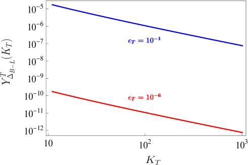
Figure 4: $B-L$ asymmetry produced by the $A_{4}$ flavor triplet ($N_{i}$) dynamics. The values $\epsilon_{T}=10^{-6}-10^{-1}$ correspond to extreme cases.

The problem of determining the final $Y^{T}_{\Delta_{B-L}}$ analytically is thus reduced to find an approximate expression for the efficiency function at $z_{i}\to\infty$ (efficiency factor). Such an expression can be derived in the strong washout regimen by: $(i)$ noting that at low temperatures $Y_{N_{i}}(z_{i})$ follows closely the equilibrium distribution, so the replacement $dY_{N_{i}}(z_{i})/dz_{i}\to dY^{\text{Eq}}_{N_{i}}(z_{i})/dz_{i}$ in eq. (56) can be done; $(ii)$ replacing the washout function $W^{T}_{ID}(z_{i})$ by $\overline{W}_{ID}(z_{i})=z_{B}\,W^{T}_{ID}(z_{i})/z$, where $z_{B}$ is the minimum of the function

$$\psi(z^{\prime},z_{i})=-\ln\left(\frac{W^{T}_{ID}(z^{\prime})}{z^{\prime}}\right)+\int_{z^{\prime}}^{z_{i}}dz^{\prime\prime}\,W^{T}_{ID}(z^{\prime\prime})\,.$$ (57)

Following this procedure the efficiency factor can be derived [26]:

$$\eta=\frac{2}{K_{T}\,z_{B}(K_{T})}\left(1-e^{-K_{T}\,z_{B}(K_{T})/2}\right)\,,$$ (58)

with

$$z_{B}(K_{T})=\frac{1}{2}\ln\left\{\frac{\pi\,K_{T}^{2}}{1024}\left[\ln\left(\frac{3125\,\pi\,K_{T}^{2}}{1024}\right)\right]^{5}\right\}\,.$$ (59)

With eqs. (58) and (59) at hand we can determine the maximum and minimum (still consistent with the measured baryon asymmetry) $B-L$ asymmetry one can get through $N_{i}$ dynamics. The results are displayed in figure 4. Particularly relevant is the maximum value $Y^{T}_{\Delta_{B-L}}\simeq 10^{-5}$ as it allows to derive an upper bound on the washout induced by $N_{4}$ dynamics.

3.4.2 $\boldsymbol{N}_{4}$ washout

The $B-L$ asymmetry produced at $z_{i}\sim 1$ remains frozen up to the temperature at which $N_{4}$ washouts become effective, $z_{4}=M_{N_{4}}/T\sim 1$. Since $N_{4}$ couples to lepton doublets via an effective five-dimensional operator the dynamics of $N_{4}$ washouts, at leading order in the couplings, involves not only the processes $N_{4}\leftrightarrow L\phi H$ but the $2\leftrightarrow 2$ $s$, $t$ and $u$ channel scatterings (see figure 5), in contrast to the standard leptogenesis scenario. The derivation of the corresponding kinetic equations in this case is tricky and requires -even at leading order in the couplings- the inclusion of $3\leftrightarrow 3$ and $2\leftrightarrow 4$ scattering processes (see ref. [10] for more details). Since $\epsilon_{N_{4}}=0$ the kinetic equations accounting for the $N_{4}$ washouts can be written according to

Figure 5: Relevant $1\leftrightarrow 3$ and $2\leftrightarrow 2$ $s$, $t$ and $u$ scattering processes accounting for the $A_{4}$ singlet washouts.

$$\frac{dY_{N_{4}}}{dz_{4}} =-\frac{1}{s(z_{4})H(z_{4})z_{4}}\left(\frac{Y_{N_{4}}(z_{4})}{Y_{N_{4}}^{\text{Eq}}(z_{4})}-1\right)\gamma_{\text{tot}}(z_{4})\,,$$ (60)

$$\frac{dY^{S}_{\Delta_{B-L}}}{dz_{4}} =-\frac{Y^{S}_{\Delta_{B-L}}}{2Y^{\text{Eq}}_{\ell}}\left[\gamma_{\text{tot}}(z_{4})+\left(\frac{Y_{N_{4}}(z_{4})}{Y_{N_{4}}^{\text{Eq}}(z_{4})}-1\right)\gamma^{s}_{2\to 2}(z_{4})\right]\,.$$ (61)

where $\gamma^{s}_{2\to 2}(z_{4})$ is the reaction density for the $2\leftrightarrow 2$ $s$-channel scattering process and $\gamma_{\text{tot}}(z_{4})$ involves the reaction densities for the full set of processes shown in figure 5, namely

$$\gamma_{\text{tot}}(z_{4})=\gamma_{1\to 3}(z_{4})+\sum_{C=s,t,u}\gamma^{C}_{2\to 2}(z_{4})\,.$$ (62)

As explained in appendix A all the reaction densities can be written in terms of the total decay width $\Gamma(N_{4}\to LH\phi)$, which we have calculated to be

$$\Gamma(N_{4}\to LH\phi)=\frac{1}{192\pi^{3}}\frac{M_{N_{4}}^{3}}{\Lambda^{2}}|y_{3}|^{2}\,.$$ (63)

In terms of the reaction densities given in (A) the kinetic equations in (60) can be rewritten in such a way they resemble eqs. (53):

$$\frac{dY_{N_{4}}}{dz_{4}} =-D_{S}(z_{4})\left(\frac{Y_{N_{4}}(z_{4})}{Y_{N_{4}}^{\text{Eq}}(z_{4})}-1\right)\,,$$

$$\frac{dY^{S}_{\Delta_{B-L}}}{dz_{4}} =-W^{S}_{ID}(z_{4})Y^{S}_{\Delta_{B-L}}\,,$$ (64)

where now the functions $D_{S}$ and $W^{S}_{ID}$ are given by

$$D_{S}(z_{4}) =\frac{1}{4g_{\star}}\,K_{S}\,z_{4}^{3}\left[K_{1}(z_{4})+\frac{3}{2}\left(S_{s}(z_{4})+S_{t}(z_{4})\right)\right]$$

$$W^{S}_{ID}(z_{4}) =\frac{1}{4}K_{S}\,z_{4}^{3}\left[K_{1}(z_{4})+\frac{3}{2}\left(\frac{Y_{N_{4}}}{Y_{N_{4}}^{\text{Eq}}}\,S_{s}(z_{4})+S_{t}(z_{4})\right)\right]\,.$$ (65)

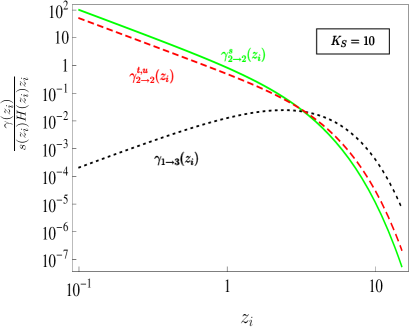
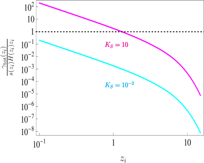
Figure 6: Reaction densities as a function of $z_{i}$ for the different processes present in $N_{4}$ washout (left panel) and total reaction densities for different values of the decay parameter $K_{S}$ (right panel). As in the standard case the strong washout (weak washout) regimen is defined according to $K_{S}\gg 1$ ($K_{S}\ll 1$).

Some words are in order regarding these equations. The relativistic degrees of freedom are $g_{\star}=118$, as in our calculations we use Maxwell-Boltzmann distributions, and the functions $S_{s,t}$ are given in eqs. (76) in the appendix. The decay parameter $K_{S}$ is defined in the same way it is defined in the case of $N_{i}$ dynamics, $K_{S}=\tilde{m}_{S}/m_{\star}$ but with

$$\tilde{m}_{S}=\frac{8\pi v^{2}}{M_{N_{4}}^{2}}\,\Gamma(N_{4}\to LH\phi)\,.$$ (66)

The presence of the $2\to 2$ scattering processes may drive the system to the strong washout regimen even when the $1\to 3$ process is slow. Thus, the appropiate definition of the strong (weak) washout regimen in this case reads:

$$\left.\frac{\gamma_{\text{tot}}(z_{i})}{s(z_{i})H(z_{i})z_{i}}\right|_{z_{i}\sim 1}>1\quad(<1\;\mbox{for weak washout})\,.$$ (67)

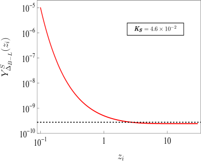
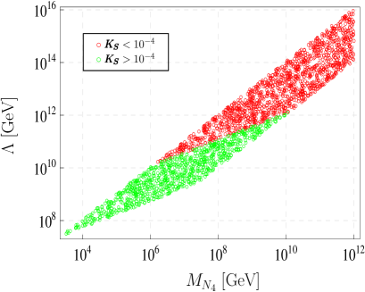
Figure 7: Washout induced by $N_{4}$ on the maximum $Y^{T}_{\Delta_{B-L}}$ (see fig. 4) generated in $N_{T}$ dynamics (left panel). The largest allowed $K_{S}$ for which the resulting $Y_{\Delta_{B}}$ still fits the measured value is $K_{S}^{\text{max}}=4.6\times 10^{-2}$, any value for which $K_{S}>K_{S}^{\text{max}}$ is excluded. On the right panel allowed regions of $\Lambda-M_{N_{S}}$ as required by the condition $K_{S}<K_{S}^{\text{max}}$.

Figure 6 (left panel) shows an example in which though $\gamma_{1\to 3}(z_{i})/s(z_{i})H(z_{i})z_{i}|_{z_{i}\sim 1}\ll 1$ the system is driven to the strong washout regimen by scattering processes. Note however that the condition $K_{S}\gg 1$ ($K_{S}\ll 1$) still determines the regimen in which the washout dynamics of $N_{4}$ takes place, as can be seen in figure 6 (right panel).

From the integration of eqs. (3.4.2) an upper bound on $K_{S}$ for a given $Y^{T}_{\Delta_{B-L}}$ can be determined by the condition of not erasing this asymmetry below $\sim 2.6\times 10^{-10}$. The maximum value $K_{S}^{\text{max}}$ is found for the largest possible $B-L$ asymmetry generated in $N_{i}$ dynamics, that as has been argued in sec. 3.4.1 we have found to be $\sim 10^{-5}$. Figure 7 (left panel) shows the final $Y^{S}_{\Delta_{B-L}}$ matches the required value $\sim 2.6\times 10^{-10}$ (for $Y^{T}_{\Delta_{B-L}}=10^{-5}$) when $K_{S}^{\text{max}}\simeq 4.6\times 10^{-2}$, any value $K_{S}>K_{S}^{\text{max}}$ will induce a washout that will damp the $B-L$ asymmetry below the allowed value.

Taking $|y_{3}|=10^{-2}$ the decay parameter $K_{S}$ becomes

$$K_{S}=12\times 10^{9}\,\left(\frac{M_{N_{4}}}{\text{GeV}}\right)\,\left(\frac{\text{GeV}}{\Lambda}\right)^{2}\,,$$ (68)

with the purpose of placing the more stringent bounds on the $\Lambda-M_{N_{4}}$ plane we fix $10^{2}<\Lambda/M_{N_{4}}<10^{4}$ and take into account the restriction $K_{S}<K_{S}^{\text{max}}$. The results are displayed in figure 7 (right panel) where the allowed $\Lambda-M_{N_{4}}$ region can be seen. Any discussion of leptogenesis in the scenario we have considered here should be done at least within that region.

4 Conclusions

In this paper we have study the necessary conditions that have to be satisfied whenever the generation of the cosmic baryon asymmetry of the Universe via leptogenesis takes place in the presence of a lepton flavor symmetry accounting for lepton mixing. In the scenario we have discussed, leptogenesis occurs in the flavor symmetric regime thus before the flavons (that trigger the breaking of the flavor symmetry) acquire vevs, accordingly the decays responsible for generating a net $B-L$ asymmetry are liable of selection rules dictated by the flavor symmetry.

In the core of the paper we exemplify how the general conditions for the generation of the baryon asymmetry, in the flavor symmetric phase, work by analysing a specific model based on the flavor symmetry $A_{4}$. We briefly discussed the low energy phenomenology of the model and studied in detail, by using the corresponding kinetics equations, the generation of the baryon asymmetry. In the model considered, due to the constraints imposed by $A_{4}$, the asymmetry proceeds through the CP violating and out-of-equilibrium decays of the heaviest RH neutrino $A_{4}$ representation. Subsequent washouts induced by the lightest $A_{4}$ representation, being potentially dangerous, were properly taken into account. Our onset shows these washouts can always be circumvented and the correct amount of baryon asymmetry can be produced.

In conclusion we have shown that under certain conditions, in models containing flavor symmetries in the lepton sector, leptogenesis can occur even in the flavor symmetric phase. The conditions we have enumerated can be regarded as a general recipe for constructing lepton flavor models in which the lepton number violating scale is above the flavor symmetry breaking scale and the generation of the baryon asymmetry proceeds via leptogenesis.

5 Acknowledgments

DAS would like to thank Luis Alfredo Munoz for discussions. DAS is supported by a FNRS belgian postdoctoral fellowship.

Appendix A Appendix: Reaction densities for $1\to 3$ and $2\to 2$ processes

In this appendix we present the relevant equations used in the calculations discussed in section 3.4.2. The thermally averaged reaction densities for $1\to 3$ and $2\to 2$ processes are given by [25]

$$\gamma_{1\to 3} =n^{\text{Eq}}_{N_{4}}\,\frac{K_{1}(z_{4})}{K_{2}(z_{4})}\,\Gamma_{1\to 3}\,,$$ (69)

$$\gamma^{C}_{2\to 2} =\frac{M_{N_{4}}^{4}}{64\,\pi^{5}\,z_{4}}\,\int_{1}^{\infty}\,dx\,\sqrt{x}\,K_{1}({z_{4}\sqrt{x}})\,\widehat{\sigma}^{C}(x)\,,$$ (70)

where $x=s/M_{N_{4}}^{2}$ (with $s$ the center of mass energy) $C=s,t,u$, $\Gamma_{1\to 3}\equiv\Gamma(N_{4}\to LH\phi)$ and $\widehat{\sigma}(x)$, the reduced cross section, defined as

$$\widehat{\sigma}(x)=2\,M_{N_{4}}^{2}\,x\,\lambda(1,x^{-1},0)\,\sigma(x)\quad\mbox{with}\quad\lambda(a,b,c)=(a-b-c)^{2}-4bc\,.$$ (71)

Neglecting the lepton doublets, Higgs and flavones masses we have found for the differential cross sections the following results:

$$\frac{d\sigma^{s}}{dt} =\frac{1}{16\pi}\,\frac{|y_{3}|^{2}}{\Lambda^{2}}\,\frac{1}{M_{N_{4}}^{2}}\frac{1}{1-x}\,,$$

$$\frac{d\sigma^{t}}{dt} =\frac{1}{16\pi}\,\frac{|y_{3}|^{2}}{\Lambda^{2}}\,\frac{1}{M_{N_{4}}^{2}}\frac{1}{(1-x)^{2}}\,\left(1-\frac{t}{M_{N_{4}}^{2}}\right)\,,$$

$$\frac{d\sigma^{u}}{dt} =\frac{1}{16\pi}\,\frac{|y_{3}|^{2}}{\Lambda^{2}}\,\frac{1}{M_{N_{4}}^{2}}\frac{1}{(1-x)^{2}}\left(x+\frac{t}{M_{N_{4}}^{2}}\right)\,.$$ (72)

Integrating over $t$ in the range $t_{-}=M_{N_{4}}^{2}(1-x)$ and $t_{+}=0$ and using the definition for the reduced cross section, eq. (71), we get

$$\widehat{\sigma}^{s}(x) =\frac{|y_{3}|^{2}}{8\,\pi}\left(\frac{M_{N_{4}}}{\Lambda}\right)^{2}\,\frac{(x-1)^{2}}{x},$$ (73)

$$\widehat{\sigma}^{t,u}(x) =\frac{|y_{3}|^{2}}{16\,\pi}\left(\frac{M_{N_{4}}}{\Lambda}\right)^{2}\,\frac{(x^{2}-1)}{x}\,.$$ (74)

With these results at hand and taking into account the expression for $\Gamma_{1\to 3}$ given in eq. (63) the different reaction densities become

$$\gamma_{1\to 3} =\frac{M_{N_{4}}^{3}}{\pi^{2}}\,,\frac{K_{1}(z)}{z}\,\Gamma_{1\to 3}\,,$$

$$\gamma^{s}_{2\to 2} =\frac{3M_{N_{4}}^{3}}{2\pi^{2}}\,\frac{S_{s}(z)}{z}\,\Gamma_{1\to 3}\,,$$

$$\gamma^{t,u}_{2\to 2} =\frac{3M_{N_{4}}^{3}}{4\pi^{2}}\,\frac{S_{t,u}(z)}{z}\,\Gamma_{1\to 3}\,,$$ (75)

where the functions $S_{s,t,u}(z)$ are given by

$$S_{s}(z)=\int_{1}^{\infty}dx\frac{(x-1)^{2}}{\sqrt{x}}\,K_{1}(z\sqrt{x})\quad\mbox{and}\quad S_{t,u}(z)=\int_{1}^{\infty}dx\frac{x^{2}-1}{\sqrt{x}}\,K_{1}(z\sqrt{x})\,.$$ (76)

References

• [1] G. Hinshaw et al. [ WMAP Collaboration ], Astrophys. J. Suppl.  180, 225-245 (2009). [arXiv:0803.0732 [astro-ph]].
• [2] A. D. Sakharov, Pisma Zh. Eksp. Teor. Fiz.  5, 32-35 (1967).
• [3] S. Davidson, E. Nardi, Y. Nir, Phys. Rept.  466, 105-177 (2008). [arXiv:0802.2962 [hep-ph]].
• [4] P. Minkowski, Phys. Lett. B 67 421 (1977); T. Yanagida, in Proc. of Workshop on Unified Theory and Baryon number in the Universe, eds. O. Sawada and A. Sugamoto, KEK, Tsukuba, (1979) p.95; M. Gell-Mann, P. Ramond and R. Slansky, in Supergravity, eds P. van Niewenhuizen and D. Z. Freedman (North Holland, Amsterdam 1980) p.315; P. Ramond, Sanibel talk, retroprinted as hep-ph/9809459; S. L. Glashow, inQuarks and Leptons, Cargèse lectures, eds M. Lévy, (Plenum, 1980, New York) p. 707; R. N. Mohapatra and G. Senjanović, Phys. Rev. Lett. 44, 912 (1980); J. Schechter and J. W. F. Valle, Phys. Rev.  D 22 (1980) 2227; Phys. Rev.  D 25 (1982) 774.
• [5] C. Hagedorn, E. Molinaro, S. T. Petcov, JHEP 0909, 115 (2009). [arXiv:0908.0240 [hep-ph]].
• [6] E. Bertuzzo, P. Di Bari, F. Feruglio, E. Nardi, JHEP 0911, 036 (2009). [arXiv:0908.0161 [hep-ph]].
• [7] D. Aristizabal Sierra, F. Bazzocchi, I. de Medeiros Varzielas, L. Merlo, S. Morisi, Nucl. Phys.  B827, 34-58 (2010). [arXiv:0908.0907 [hep-ph]].
• [8] R. G. Felipe, H. Serodio, Phys. Rev.  D81, 053008 (2010). [arXiv:0908.2947 [hep-ph]].
• [9] D. Aristizabal Sierra, M. Losada, E. Nardi, Phys. Lett.  B659, 328-335 (2008). [arXiv:0705.1489 [hep-ph]].
• [10] D. Aristizabal Sierra, L. A. Munoz, E. Nardi, Phys. Rev.  D80, 016007 (2009). [arXiv:0904.3043 [hep-ph]].
• [11] C. D. Froggatt, H. B. Nielsen, Nucl. Phys.  B147, 277 (1979).
• [12] G. Altarelli, F. Feruglio, Rev. Mod. Phys.  82 (2010) 2701-2729. [arXiv:1002.0211 [hep-ph]].
• [13] E. E. Jenkins, A. V. Manohar, Phys. Lett.  B668, 210-215 (2008). [arXiv:0807.4176 [hep-ph]].
• [14] Riazuddin, [arXiv:0809.3648 [hep-ph]].
• [15] D. Aristizabal Sierra, Federica Bazzocchi, Ivo de Medeiros Varzielas, 1112.1843[hep-ph], to appear in Nucl.Phys B.
• [16] I. de Medeiros Varzielas, R. Gonzalez Felipe and H. Serodio, Phys. Rev. D 83, 033007 (2011) [arXiv:1101.0602 [hep-ph]].
• [17] T. Schwetz, M. Tortola, J. W. F. Valle, [arXiv:1108.1376 [hep-ph]].
• [18] G. C. Branco, A. J. Buras, S. Jager, S. Uhlig, A. Weiler, JHEP 0709, 004 (2007). [hep-ph/0609067].
• [19] G. Altarelli, F. Feruglio, Y. Lin, Nucl. Phys.  B775 (2007) 31-44. [hep-ph/0610165].
• [20] F. Bazzocchi, L. Merlo, S. Morisi, Phys. Rev.  D80 (2009) 053003. [arXiv:0902.2849 [hep-ph]].
• [21] L. Covi, E. Roulet, F. Vissani, Phys. Lett.  B384, 169-174 (1996). [hep-ph/9605319].
• [22] F. -X. Josse-Michaux, E. Molinaro, [arXiv:1108.0482 [hep-ph]].
• [23] D. Aristizabal Sierra, J. F. Kamenik, M. Nemevsek, JHEP 1010, 036 (2010). [arXiv:1007.1907 [hep-ph]].
• [24] E. Nardi, J. Racker, E. Roulet, JHEP 0709, 090 (2007). [arXiv:0707.0378 [hep-ph]].
• [25] G. F. Giudice, A. Notari, M. Raidal, A. Riotto, A. Strumia, Nucl. Phys.  B685, 89-149 (2004). [hep-ph/0310123].
• [26] W. Buchmuller, P. Di Bari, M. Plumacher, Annals Phys.  315, 305-351 (2005). [hep-ph/0401240].