Weak Turbulence in the Magnetosphere: Formation of Whistler Wave Cavity by Nonlinear Scattering

Abstract

We consider the weak turbulence of whistler waves in the in low-$\beta$ inner magnetosphere of the Earth. Whistler waves with frequencies, originating in the ionosphere, propagate radially outward and can trigger nonlinear induced scattering by thermal electrons provided the wave energy density is large enough. Nonlinear scattering can substantially change the direction of the wave vector of whistler waves and hence the direction of energy flux with only a small change in the frequency. A portion of whistler waves return to the ionosphere with a smaller perpendicular wave vector resulting in diminished linear damping and enhanced ability to pitch-angle scatter trapped electrons. In addition, a portion of the scattered wave packets can be reflected near the ionosphere back into the magnetosphere. Through multiple nonlinear scatterings and ionospheric reflections a long-lived wave cavity containing turbulent whistler waves can be formed with the appropriate properties to efficiently pitch-angle scatter trapped electrons. The primary consequence on the Earth’s radiation belts is to reduce the lifetime of the trapped electron population.

I Introduction

The dynamics of whistler wave packets in the inner magnetosphere have been investigated using linear ray tracing for decades Haselgrove (1955); Kimura (1966); Lauben, Inan, and Bell (2001); Santolik et al. (2001); Bornik, Inan, and Bell (2003). These studies are important in understanding the lifetime of trapped energetic electrons in the Earth’s radiation belts because pitch-angle scattering by electromagnetic whistler waves into the loss-cone can be the dominant loss mechanismAbel and Thorne (1998). The rate of pitch-angle scattering is a sensitive function of the spatial, spectral, and wave-normal distributions of the wave energy density, and therefore mechanisms that control the distribution of wave energy are important. Recently the results of Hasegawa and Chen (1975) and Tripathi, Grebogi, and Liu (1977) have been extended to demonstrate that, through nonlinear (NL) induced scattering by thermal electrons in low-$\beta$ plasmas, quasi-electrostatic lower-hybrid waves can scatter into electromagnetic whistler wavesGanguli et al. (2010); Mithaiwala et al. (2011). In this paper we report on initial efforts to incorporate this NL mechanism into the calculation of the propagation of whistler waves in the plasmasphere. We find that when the turbulent wave energy density exceeds a threshold, NL scattering can scatter waves that have exhausted their usefulness for pitch-angle scattering back into useful waves capable of further pitch angle scattering. We suggest a weak turbulence framework for incorporating these effects into ray tracing calculations. This framework is a natural extension of linear techniques such as ray tracing and quasi-linear diffusion that have been the workhorse of radiation belt physics for decades.

Magnetospherically reflecting whistlers (MRW) are whistler waves, possibly originating from lightning strikes, whose ray paths in the magnetosphere roughly follow magnetic field lines, reflecting many times between the magnetic poles. Waves originating in the ionosphere propagate to higher and higher altitude and the perpendicular component of the wave vector increasesEdgar (1976). Based on linear theory there are two important physical effects that limit the degree of influence that MRW are predicted to have on the lifetime of trapped energetic electrons. First, linear damping of whistler waves depends strongly on the perpendicular wavelength (increasing as $k_{\perp}^{2}$). Whistler waves have a significant parallel electric field when the perpendicular wavelength becomes comparable with the electron skin depth. This parallel electric field is the driving force of linear Landau damping (resonant interactions with electrons) as well as collisional damping. Also, electron drift $\boldsymbol{E}\times\boldsymbol{B}$ energy increases as the square of $k_{\perp}$. Thus as whistler waves propagate from their source region and the perpendicular component of the wave vector becomes larger the linear damping of the waves becomes stronger. Second, the rate of pitch-angle scattering of trapped electrons depends strongly on the perpendicular wavelength. As the perpendicular wavelengths become shorter than the electron skin depth the whistler wave becomes more electrostatic in nature (more lower-hybrid like) and thus the magnetic component (which pitch-angle scatters through the Lorentz force, $(e/c)\boldsymbol{v}\times\boldsymbol{B}$) is reduced. In this article we will demonstrate that when the energy density of whistler waves is large enough, NL induced scattering can return a portion of short-wavelength quasi-electrostatic lower-hybrid waves back into long-wavelength electromagnetic whistler waves which are less damped and more effective at pitch-angle scattering.

The scattered waves (with smaller $k_{\perp}$) have only a slightly lower frequency than the original whistler waves, but the direction of $\boldsymbol{k}$ and their trajectory through the magnetosphere can be dramatically altered Ganguli et al. (2010); Mithaiwala et al. (2011). A portion of the scattered waves can be returned back to the ionosphere, and some of these waves will retrace the original ray paths back to the magnetosphere. These scattered waves are then able to efficiently pitch-angle scatter relativistic electrons once again. Through multiple NL scatterings in the magnetosphere and reflections in the ionosphere a cavity containing turbulent whistler waves may be formed that is more long-lived than would be predicted without NL scattering, because the effective $k_{\perp}$ and thus linear damping rate is reduced.

In section II we review the dynamics of whistler wave packets without NL scattering from the ionosphere into the magnetosphere and describe our assumptions in characterizing these trajectories. In section III, we describe how we include the effects of NL induced scattering into the dynamics of whistler wave packets. In section IV we describe how a long-lived wave energy cavity may be formed due to induced NL scattering and describe some of the basic properties of this cavity. In section V we discuss the role that this newly postulated wave cavity may play in radiation belt physics and outline future efforts to improve our understanding of the properties of the wave cavity.

II Ray Tracing Whistler Waves

II.1 Model Assumptions

To model the dynamics of whistler wave packets in the magnetosphere/ionosphere we use the following dispersion relation applicable to cold plasmas for waves with frequencies between the proton and electron cyclotron frequenciesGanguli et al. (2010),

$$\omega^{2}=\left[\frac{\bar{k}_{\|}^{2}}{1+\bar{k}_{\perp}^{2}}\Omega_{e}^{2}+\omega_{LH}^{2}\right]\frac{\bar{k}^{2}}{1+\bar{k}^{2}}$$ (1)

where, $\omega_{LH}^{2}=\sum_{ions}\omega_{ps}^{2}/(1+\omega_{pe}^{2}/\Omega_{e}^{2})$ is the lower-hybrid frequency, $\omega_{ps}$ is the plasma frequency, and $\Omega_{s}$ the cyclotron frequency of species $s$. In Fig. 1, we show contours of constant frequency in $(\bar{k}_{\|},\bar{k}_{\perp})=(k_{\|},k_{\perp})c/\omega_{pe}$ space calculated from Eq. 1. In the lower right corner ($\bar{k}_{\perp}>1$ and $\bar{k}_{\|}<\bar{k}_{\perp}(m_{e}/m_{i})^{1/2}$) are the quasi-electrostatic lower-hybrid waves with $\omega^{2}\simeq\omega_{LH}^{2}$, in the upper left corner ($\bar{k}_{\perp}<1$ and $\bar{k}_{\|}>(m_{e}/m_{i})^{1/2}$) are the electromagnetic whistlers with $\omega^{2}\simeq\bar{k}_{\|}^{2}\bar{k}^{2}\Omega_{e}^{2}$, and in the lower left corner ($\bar{k}_{\perp}<1$ and $\bar{k}_{\|}<(m_{e}/m_{i})^{1/2}$) are the magnetosonic waves with $\omega^{2}\simeq\bar{k}^{2}\omega_{LH}^{2}\simeq k^{2}V_{A}^{2}$, where $V_{A}^{2}=B^{2}/(4\pi n_{i}m_{i})$ is the Alfvén velocity.

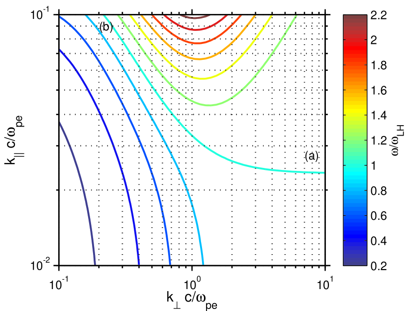
Figure 1: Contours of constant $\omega$ normalized to $\omega_{LH}$ calculated from Eq. 1

We use magnetic coordinates $(\chi,\alpha,\beta)$ where $\boldsymbol{B}=\boldsymbol{\nabla}\chi=\boldsymbol{\nabla}\alpha\times\boldsymbol{\nabla}\beta$ with a pure dipole field such that,

$$\chi=-\frac{M\cos(\theta)}{r^{2}}\qquad\alpha=\frac{M\sin^{2}(\theta)}{r}\qquad\beta=\phi$$ (2)

where $M=-8\times 10^{25}$ G/cm³ is the earth’s dipole moment. In these coordinates the components of the group velocity may be calculated,

$$\begin{split}\dot{\chi}&=\frac{\partial\omega}{\partial k_{\chi}}=\frac{1}{1+\bar{k}^{2}}\left[\frac{\bar{k}^{2}}{1+\bar{k}_{\perp}^{2}}\Omega_{e}^{2}+\frac{\omega^{2}}{\bar{k}^{2}}\right]\frac{c^{2}}{\omega_{pe}^{2}}\frac{g^{\chi\chi}k_{\chi}}{\omega}\\ \dot{\alpha}&=\frac{\partial\omega}{\partial k_{\alpha}}=\frac{1}{1+\bar{k}^{2}}\left[-\frac{\bar{k}_{\|}^{2}\bar{k}^{2}}{\left(1+\bar{k}_{\perp}^{2}\right)^{2}}\Omega_{e}^{2}+\frac{\omega^{2}}{\bar{k}^{2}}\right]\frac{c^{2}}{\omega_{pe}^{2}}\frac{g^{\alpha\alpha}k_{\alpha}}{\omega}\\ \dot{\beta}&=\frac{\partial\omega}{\partial k_{\beta}}=\frac{1}{1+\bar{k}^{2}}\left[-\frac{\bar{k}_{\|}^{2}\bar{k}^{2}}{\left(1+\bar{k}_{\perp}^{2}\right)^{2}}\Omega_{e}^{2}+\frac{\omega^{2}}{\bar{k}^{2}}\right]\frac{c^{2}}{\omega_{pe}^{2}}\frac{g^{\beta\beta}k_{\beta}}{\omega}\end{split}$$ (3)

where $g^{\chi\chi}$, $g^{\alpha\alpha}$, and $g^{\beta\beta}$ are components of the metric tensor.

To model the density in the magnetosphere we use a simple analytical two ion species model that was designed to capture the main features of a standard ionospheric density profile relevant to whistler wave propagations. The densities are all proportional to the magnetic field, $n_{s}=f_{s}(r)B$, multiplied by a function that depends only on the radius. The multiplying functions are defined by,

$$\begin{split}f_{e}&=f_{e0}(r-r_{0})+f_{e1}(1+\tanh(\frac{(r-r_{1})}{\Delta r_{1}}))\exp(-\frac{r}{\Delta r_{2}})\\ f_{H}&=\left[1/2(1+\tanh(\frac{r-r_{H1}}{\Delta r_{H1}})\right]f_{e}\\ f_{O}&=1-f_{H}\end{split}$$ (4)

with the values of parameters determined by a fit to a night-time ionosphere profile. The densities and lower-hybrid frequencies are plotted as a function of altitude in the upper ionosphere in Fig. 2.

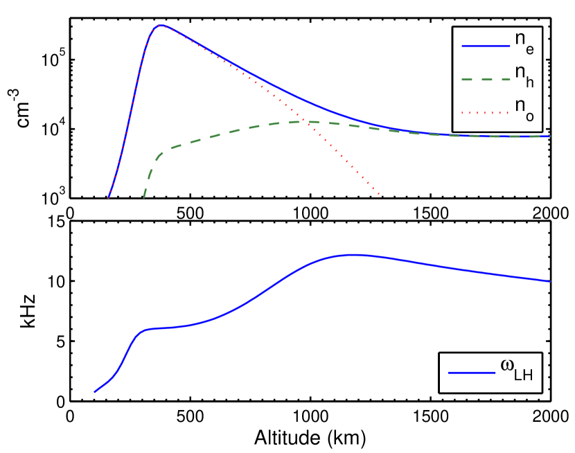
Figure 2: Densities (top) and lower-hybrid frequency (bottom) vs altitude in model ionosphere.

In addition to following the dynamics of wave-packets through $(\boldsymbol{x},\boldsymbol{k})$ space, we also follow the amount of energy lost due to linear damping. Since the region of interest (lower magnetosphere) is a cold plasma ($T_{e}\sim 0.1-0.5$ eV) Landau damping by the thermal part is completely negligible compared to collisional damping. There sometimes exists a population of suprathermal electrons that can be in resonance with whistler wavesBell et al. (2002), however this damping is smaller than the collisional damping we consider (see appendix A). We include the effects of linear collisional (electron-ion) damping by using the approximate damping rate,

$$\gamma_{L}=-\frac{\nu_{ei}}{2}\frac{2\bar{k}_{\|}^{2}+\bar{k}_{\perp}^{2}}{1+\bar{k}_{\perp}^{2}}$$ (5)

where $\nu_{ei}=3\times 10^{-5}n_{e}T_{e}^{-3/2}\,({\rm sec}^{-1})$, which requires a temperature for which we use a simple two temperature model profile given by,

$$T_{e}=0.1+1/5(1+\tanh(\frac{\textrm{alt}-1100}{200}))\qquad\textrm{eV}$$ (6)

where alt is the altitude in km.

For this initial work we confine ourselves to considering sources in the ionosphere, however, we note that geomagnetic storms and chorus emissions are examples of potential sources from the outer magnetosphere. As for sources in the ionosphere that could generate whistler wave power there are many candidates, e.g. lightning, VLF transmitters, and velocity ring distributions generated naturally or man made such as in the Buaro experimentKoons and Pongratz (1981) or an envisioned future experiment Ganguli et al. (2007).

II.2 Linear Dynamics of Whistler Waves

Generally speaking, whistler waves with small wave normal angles propagate from their source region roughly along magnetic field lines, reflecting between the magnetic poles and increasing the value of the perpendicular wave vector. The obliqueness of the wave allows for cross-field propagation so that wave packets initiated in the ionosphere propagate to higher and higher altitude (and L-shell). Eventually the wave-packet reaches an L-shell greater than the L-shell at which the frequency of the wave matches the lower-hybrid frequency and the radial group velocity reverses. By this time (a few seconds) the wave packet has a large perpendicular wave vector and follows the field line more closely. Its radial group velocity is relatively small and the wave packet slowly makes its way back to the lower-hybrid resonant surface. Fig. 3 shows the dynamics of a single wave packet, characteristic of packets that reach the magnetosphere, launched from an ionospheric source at an altitude of 1100 km at 30^∘ N and midnight local time with a frequency of 6 kHz (where the local lower hybrid frequency is about 12 kHz). The model ionosphere/magnetosphere is independent of the azimuthal coordinate and thus the azimuthal component of the wave vector is a constant of motion. Therefore the wave-packet in figure 3 which was launched with no azimuthal component of the wave vector is confined to the meridian it began in. In Figure 4 we show the trajectory of a wave packet launched from the same point in space and the same frequency, but with a component of the wave vector out of the noon-midnight plane. In this case the packet initially has a significant group velocity in the azimuthal direction, but the packet quickly settles down into a plane of constant local time and does not proceed to encircle the earth. These packets last almost 10 seconds before the initial energy is reduced by 99% by collisional damping.

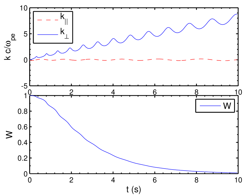
Figure 3: Wave packet trajectory in x-z plane for 6 kHz wave launched from 1100 km altiitude and 30^∘N (top) and evolution of $\boldsymbol{k}$ and energy (bottom).

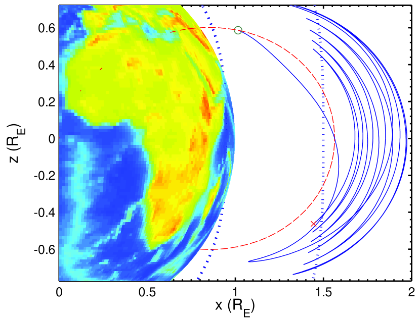
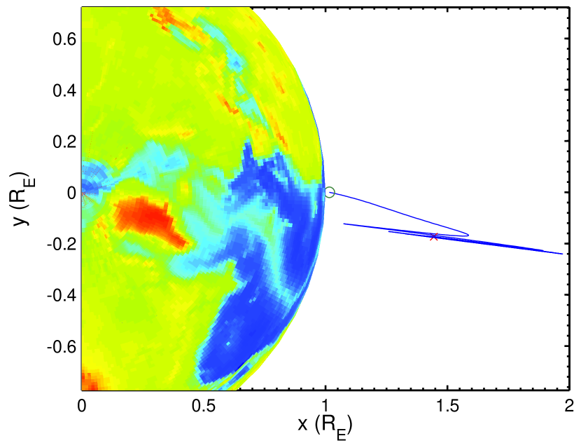
Figure 4: Wave packet trajectory for 6 kHz wave launched from 1100 km altitude and 30^∘N with component of $\boldsymbol{k}$ in azimuthal direction. Top is x-z plane. Bottom is x-y plane.

III Theory

In the framework of weak turbulence theory the dynamics of whistler wave packets in the magnetosphere may be described by the wave-kinetic equation which gives the evolution of the whistler wave packet “number density” $N=W/\omega$ where $W$ is the energy density and $\omega$ is the frequency,

$$\frac{\partial N}{\partial t}+\boldsymbol{\nabla}_{r}\cdot\left(\frac{{\rm d}\boldsymbol{r}}{{\rm d}t}N\right)+\boldsymbol{\nabla}_{k}\cdot\left(\frac{{\rm d}\boldsymbol{k}}{{\rm d}t}N\right)=\gamma_{NL}N+2\gamma_{L}N+Q$$ (7)

where the left side of (7) expresses the conservation of phase volume in $(\boldsymbol{r},\boldsymbol{k})$ space of wave packets (Liouville theorem). The evolution of the wave packets through phase space $(\boldsymbol{x},\boldsymbol{k})$ are given by the usual ray tracing equations,

$$\frac{{\rm d}\boldsymbol{r}}{{\rm d}t}=\frac{\partial\omega}{\partial\boldsymbol{k}}\;\rm{and}\;\frac{{\rm d}\boldsymbol{k}}{{\rm d}t}=-\frac{\partial\omega}{\partial\boldsymbol{r}}.$$ (8)

On the right hand side of Eq. (7) $Q$ is a source of wave energy e.g. lightning discharges, chorus waves propagating into the plasmasphere, VLF transmitters, etc., $\gamma_{L}$ is the linear damping/growth rates which along with the usual quasi-linear equations for the distribution of particles would give the complete self-consistent linear dynamics of waves and particles. The new physics is contained in $\gamma_{NL}$, the NL induced scattering rateGanguli et al. (2010); Mithaiwala et al. (2011),

$$\gamma_{NL}=\frac{1}{\omega_{k2}}\frac{\bar{k}_{2}^{2}}{1+\bar{k}_{2}^{2}}\sum_{k_{1}}\frac{|E_{k1}|^{2}}{4\pi nm_{e}}\frac{\left|\boldsymbol{k}_{1}\times\boldsymbol{k}_{2}\right|^{2}_{\|}}{k_{\perp 1}^{2}k_{\perp 2}^{2}}\\ \times\frac{(\boldsymbol{k}_{2}-\boldsymbol{k}_{1})^{2}\bar{k}_{1}^{2}}{1+\bar{k}_{1}^{2}}\frac{{\rm Im}\epsilon^{e}_{k_{1}-k_{2}}|\epsilon^{i}_{k_{1}-k_{2}}|^{2}}{\left|\epsilon^{e}_{k_{1}-k_{2}}+\epsilon^{i}_{k_{1}-k_{2}}\right|^{2}}$$ (9)

where $\epsilon^{e,i}_{k_{1}-k_{2}}$ are the plasma electron and ion susceptibilities, and $E_{k1}$ is related to $N_{k1}$ (detailed discussion is contained in the appendix). $\gamma_{NL}$ is to be interpreted as the rate of change of the energy contained in waves with wave vector $(\bar{k}_{\|},\bar{k}_{\perp})$ due to all other waves with different frequencies and wave vectors with $(\bar{k}_{\|1},\bar{k}_{\perp 1})$. This formula was derived for isothermal, $T_{e}\simeq T_{i}$, low-$\beta$ magnetospheric plasmas from the drift kinetic equation for electrons with a fluid response for ions. It is the electromagnetic generalization of the lower-hybrid induced scattering rate found by Hasegawa and Chen (1975) and used in tokamak heating scenarios. The scattering rate can be physically understood as the landau damping of thermal electrons by the electric field structure created by the beating of two waves. It is important to point out that the nature of this electric field structure is inherently 3D as can be seen by the presence of the cross product of two perpendicular wave vectors and the parallel components of the wave vectors within the plasma dispersion function. 2D simulations with the simulation plane perpendicular to the magnetic field, or 2D simulations with the magnetic field along one of the simulation axes will miss this fast scattering rate Ganguli et al. (2010) and will generally see only a slower scalar nonlinearity. Three-dimensional simulations, or 2D simulations where the magnetic field is oblique to the simulation plane are required. For the purposes of this paper, the importance of this three-dimensionality is that NL scattering allows wave packets with components of the wave vector in a meridional plane to scatter out of the plane as will be shown in the next section. Equation (9) was developed in the framework of weak turbulence theory, which considers the NL coupling of linear waves with stochastic uncorrelated phases, so that all waves are solutions to the same linear dispersion relation, and hence the NL induced scattering essentially redistributes energy in $\boldsymbol{k}$-spaceSagdeev and Galeev (1969); Davidson (1972).

From Eq. (9) we see that the NL scattering rate is largest when the change in frequency $\Delta\omega_{k1}\simeq v_{te}|k_{\|1}-k_{\|}|$, and since the electron temperature in the plasmasphere is of the order of an electron volt (which gives an electron thermal speed of about 4$\times 10^{7}$ cm/s) then the change in frequency due to a scattering is much smaller than the change in wave vector. This allows one to view the lines of constant frequency in Fig 1 as all of the possible waves that a given wave could scatter into. For example, if we have a wave that is lower-hybrid like, marked with point (a) in the figure, it may scatter into a whistler wave, marked with point (b) in the figure. This has important consequences for the influence of whistler waves on the radiation belts, namely that waves that have already become lower-hybrid like due to the evolution of individual wave packets in a dipole field as predicted by ray tracing, have an opportunity to become whistler waves again.

To gain a detailed understanding of the effects of the NL scattering on the propagation of wave power in the radiation belts a self-consistent solution, either numerical or analytical, to the wave-kinetic equation is needed. Since this is beyond the scope of this work, we adopt a test wave-packet approach to investigate the effects of NL scattering and thus solutions to Eq. 7.

IV Effect of NL Scattering on Wave Packet Trajectories

In this section we describe how a cavity in the magnetosphere may be formed when the wave energy density exceeds a threshold, we describe the properties of the cavity, and estimate the influence the formation of the cavity will have on the trajectory and fate of whistler wave packets and on the lifetime of trapped energetic electrons.

IV.1 Access to magnetospheric cavity from ionospheric source

We choose a source region in the ionosphere or in the transition region between the ionosphere and the magnetosphere (see Table 1) and suppose that the whistler energy flux is nearly monochromatic and isotropic in $\boldsymbol{k}$ space. Launching whistler wave packets with the same frequency, from the same location in space, with random directions of the wave vector we can build up a background. By choosing a random direction for the wave vector many packets will immediately be lost by propagation towards the Earth’s surface, and another percentage of packets will be lost by closely following the magnetic field lines and reaching the Earth’s surface in the opposite hemisphere. In addition, some of the packets are trapped by the steep electron density gradient (closest to the peak in density near 400 km), and because of the high density are quickly collisionally damped. We call these packets ducted. The percentages of packets for the different cases are listed in table 1. In Fig. 5 we show the trajectories of wave packets that enter the magnetospheric cavity launched from 1100 km altitude, 30^∘ N with a frequency of 6 kHz. This figure gives an idea of the three dimensional geometry of the cavity which will be further discussed in the section IV.3. In Fig. 6 we show a sample of wave packet trajectories launched from 500 km altitude with a frequency of 6 kHz that are lost to the Earth. We find that the percentage of packets that enter the magnetospheric cavity increases for the higher altitude and latitude initial conditions, mainly because more packets that travel to the southern hemisphere are refracted back into the magnetospheric cavity.

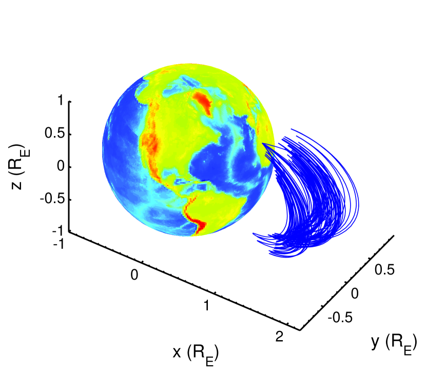
Figure 5: Trajectories of wave packets that enter magnetospheric cavity launched from 1100 km altitude, 30^∘ N, with a frequency of 6 kHz.

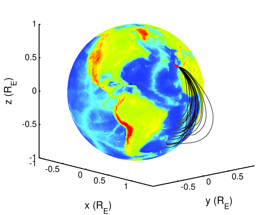
Figure 6: Trajectories of wave packets that are lost to the Earth launched from 500 km altitude, 30^∘ N, with a frequency of 6 kHz. Red paths are lost to the Northern hemisphere. Black paths are lost to the Southern hemisphere.

IV.2 Threshold for NL scattering

We estimate the threshold in wave energy density necessary for NL induced scattering to play an important role in the evolution of whistler waves. To do this we suppose that the source lasts for a time much longer than the bounce time of wave packets between the magnetic poles and follow wave packets until they reach the surface of the earth or their energy density reduces by 99% while oscillating near the lower hybrid surface in the magnetosphere. From this background of waves we can form a grid in space and calculate ensemble averages of useful quantities such as $\bar{k}_{\perp}$. We define the following average,

$$\left\langle X\right\rangle(\boldsymbol{x}_{i})=\frac{\sum_{\boldsymbol{x}\in\boldsymbol{x}_{i}}WX}{\sum_{\boldsymbol{x}\in\boldsymbol{x}_{i}}W}$$ (10)

where $W$ is the energy of the particular wave-packet. In Figure 7 we plot such quantities from an ensemble of waves launched from 500 km altitude with a frequency of 4 kHz (63% of the LH frequency). Since we assume that the source lasts for 30 seconds we record all equatorial plane crossings at different times to form this average.

Next, we estimate the NL scattering rate (Eq. 9) by assuming a broad band of turbulence, $\delta\omega\sim\omega$, and replace the summation with integrations. Using the condition that the integrand is dominated by the condition $\zeta\sim 1$, and the change in frequency is comparable to the ion-cyclotron frequency (see Appendix ) the NL scattering rate may be approximated as,

$$\gamma_{NL}\sim\omega_{LH}\left(\frac{M}{m}\right)^{3/2}\frac{\omega}{\delta\omega}\frac{\left\langle\bar{k}_{\perp}\right\rangle^{8}}{\left(1+\left\langle\bar{k}_{\perp}\right\rangle^{2}\right)^{2}}\frac{B^{2}_{1}}{B_{0}^{2}}$$ (11)

Then, from the form of Eq. (7) we expect that NL scattering will dominate linear damping when the energy density is large enough such that $\gamma_{NL}>\gamma_{L}$. Performing the same averaging procedure on the collisional damping rate, Eq. (5), we can estimate the NL threshold as,

$$\left(\frac{B_{1}^{2}}{8\pi}\right)_{th}\sim\frac{1}{2}\frac{\nu_{ei}}{\omega_{LH}}\left(\frac{m}{M}\right)^{3/2}\left(\frac{1+\left\langle\bar{k}_{\perp}\right\rangle^{2}}{\left\langle\bar{k}_{\perp}\right\rangle^{6}}\right)\frac{\delta\omega}{\omega}\frac{B_{0}^{2}}{8\pi}$$ (12)

in the limit $\left\langle\bar{k}_{\|}\right\rangle<\left\langle\bar{k}_{\perp}\right\rangle$ which is justified by the calculations leading to Fig. 7. Then taking the peak $\left\langle\bar{k}_{\perp}\right\rangle$ from the ray tracing calculations, and estimating $\delta\omega/\omega\sim 1/2$ we can then estimate the NL threshold energy. We find that the energy density to reach threshold corresponds to magnetic field amplitudes of about 100 pT. It should be pointed out that this estimated threshold is of the same order of magnitude as the observed amplitude of plasmaspheric hiss Thorne et al. (1973); Smith et al. (1974). Thus it can play an important role in such phenomenon as radiation belt slot formation and it can effect theories of the source of plasmaspheric hiss. As we will show in the next section NL scattering can significantly effect the wave propagation.

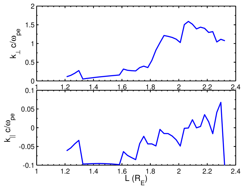
Figure 7: Ensemble average of the perpendicular wave vector for waves launched from 500 km altitude with a frequency of 4 kHz.

IV.3 Properties of Wave Energy Cavity

In the previous sections we computed the accessiblity of whistler waves into the magnetosphere and the threshold in local wave energy density necessary for NL scattering to be important. Now we use ray tracing calculations to estimate the volume of the cavity so that we may estimate the energy necessary to be input to the cavity to achieve sufficient NL scattering. We launch 1000 wave packets into the magnetosphere and compute the maximum extent in the azimuthal direction (in units of hours, i.e. 12 hours is 180 degrees), and the maximum extent in latitude. In table 2 we summarize the results of our calculations. In general we find that the azimuthal extent of the cavity decreases with increasing frequency and altitude, and is fairly insensitive to latitude. The meridional extent of the cavity increases with the latitude and altitude of the whistler launch point and frequency. To compute the maximum radial extent we find the the maximum radial value achieved by at least 10% of the packets. The reason for this distinction is that for the higher latitude cases there are a minority of packets ($<10\%$ that can achieve large radial excursions on the first or second magnetospheric reflection). We find that in general the maximum radial extent decreases with frequency and increases with latitude. Also included in the table is an estimate of the volume of the cavity where the minimum radius of the cavity is always taken to be 1.4 $R_{E}$. From these volume estimates we can then use the wave energy density necessary to overcome the NL threshold and arrive at the necessary total energy to achieve threshold. This is indicated in the final column of table 2.

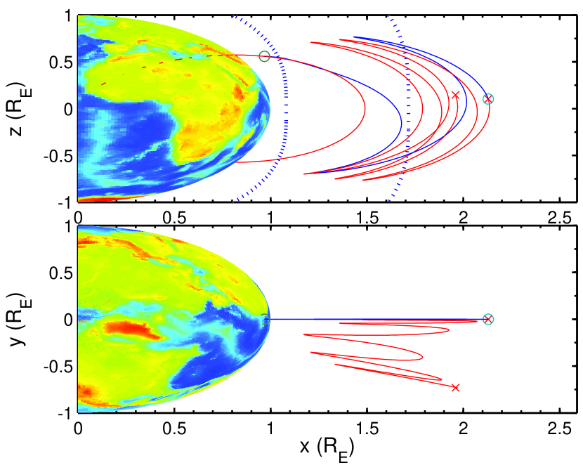
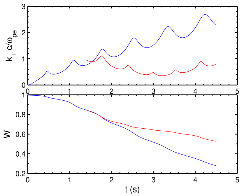
Figure 8: Wave packet trajectory (top) for 4 kHz wave launched from 750 km altiitude and 30^∘N (blue) with wave vector confined to meridional plane and scattered after 1.4 seconds (red). Perpendicular wave vector and energy of wave as a function of time (bottom), blue indicates unscattered wave and red is scattered wave.

Next we describe an example of a single scattering. For this purpose we assume that enough wave energy density is present in the system so that a wave packet may scatter. In Fig. 8 we show the trajectory (top in blue) of a wave packet with a frequency of 4 kHz launched from 750 km altitude at 30^∘ N latitude. This wave packet has the wave vector in the noon-midnight meridian so that the wave packet is confined to the same meridian. After 1.4 seconds the wave packet has increased its value of $\bar{k}_{\perp}$ to about unity and experiences a large angle scattering, such that the new wave packet has a component of the wave vector out of the meridian plane. The new scattered packet also has $\bar{k}_{\perp}\sim 1$, but this packet is on a different trajectory so that $\bar{k}_{\perp}$ decreases in time for a while before returning back to the magnetospheric lower hybrid surface and increasing $\bar{k}_{\perp}$ again. This reduction in $\bar{k}_{\perp}$ allows for the energy density in the wave to be almost a factor of 2 larger than the energy density found in the packet without scattering (and a subsequent reduction in the final value of $\bar{k}_{\perp}$).

Finally, we discuss the effects of many scatterings. In figure 8 we show what happens to a particular wave packet that is scattered which says in the magnetospheric cavity. However not all packets stay in the cavity. Some are lost to the Earth, and others experience large linear damping. To begin to quantify this energy loss we define a whislter wave albedo that we calculate by launching whistler wave packets with random directions for the wave vectors from inside the magnetospheric cavity and integrating the ray tracing equations for a specified time and then comparing the total energy of the packets at this time to the total initial energy in the packets. Thus, the albedo is defined as,

$$Albedo=\frac{\sum W_{t=t_{end}}}{\sum W_{t=0}},$$ (13)

where the numerator does not include packets that are lost to the earth. A good choice for the ending time in the albedo calculation would be the time a particular packet spends before it’s next “collision”, i.e. $1/\gamma_{NL}$. For simplicity, we chose the energy density such that the NL collision time was 1.5 seconds for all packets. In Fig. 9 we show a sample of ray tracing calculations for which the wave packets remain in the cavity, with their initial conditions marked by circles and their termination points by x’s. Performing these kinds of calculations for all of the cases we considered we summarize the results in table 3. In general we find that the albedo decreases with increasing frequency, is fairly insensitive to the altitude of release, and is larger for the higher latitude release case. In addition to the albedo the table shows the percentage of packets that are lost to the Earth. In all cases this is the dominant source of energy loss.

Another feature of many NL scatterings is that the size of the cavity can increase, this feature can be seen in the example figure 9, where the size of the new cavity can be seen by the ray trajectories in blue overlaid on the original size of the cavity estimated as thick red line in the figure. One mechanism for increasing the size is that packets which have become confined to a particular meridian may be scattered such that they propagate azimuthally. An individual case can be seen in Fig. 8. In table 3 we estimate the dimensions of the cavity after a first scattering.

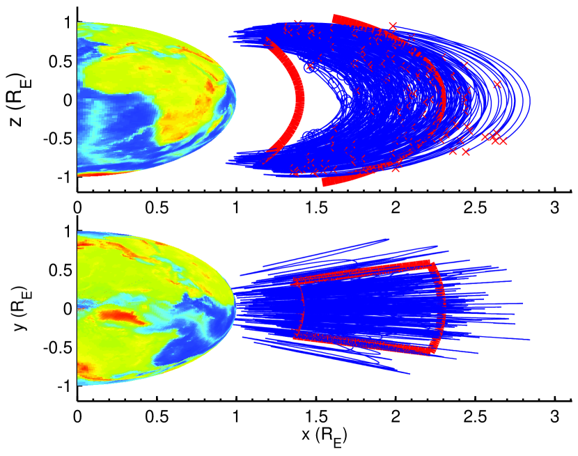
Figure 9: Scattered wave packet trajectories for 6 kHz wave launched from 1100 km altiitude and 30^∘N. Solid thick lines (red) indicate approximate boundary of unscattered cavity.

IV.4 Effect of Cavity Formation on Energetic Trapped Electrons

There are three main components to enhancing the pitch-angle scattering of energetic trapped electrons by NL scattering of whistler waves. The first is that the energy density of the whistler waves from a given source can be enhanced above the value predicted by ray tracing without NL scattering. This was demonstrated in figure 8, a corollary of this phenomenon is that the waves can live longer in the cavity with NL scattering than without, and this was discussed in relation to the albedo of the Earth. The final ingredient is that the average wave-normal angle can be decreased, which enhances the pitch-angle scattering in the following way.

The pitch-angle diffusion coefficient is approximately given by,

$$D_{\theta\theta}\sim\frac{\Omega_{e}}{\gamma_{R}}\frac{W}{B_{0}^{2}/(8\pi)}\left(\frac{J_{1}(\sigma)}{\sigma}\right)^{2}$$ (14)

where $\sigma=k_{\perp}v_{\perp}/(\Omega_{e}/\gamma_{R})$ and $\gamma_{R}$ is the relativistic factor. The cyclotron resonance condition ($\omega-k_{\|}v_{\|}=\Omega_{e}/\gamma_{R}$) for relativistic electrons and whistler waves gives $k_{\|}c\cos(\theta)\simeq\Omega_{e}/\gamma_{R}$ where $\theta$ is the electron pitch-angle. With this condition the argument of the Bessel function becomes $\sigma\simeq(k_{\perp}/k_{\|})\tan(\theta)$ which quickly becomes large due to linear ray tracing of wave packets. In this limit, $\sigma>>1$, the pitch-angle diffusion coefficient becomes,

$$D_{\theta\theta}\sim k_{\|}c\left(\frac{k_{\|}}{k_{\perp}}\right)^{3}\frac{W}{(B_{0}^{2}/(8\pi)}\cos(\theta)\cot^{3}(\theta)$$ (15)

which can be very small. What this formula shows, is that without NL scattering of whistlers the time with which a wave packet can effectively scatter relativistic electrons is very short. However, with NL scattering a population of packets can be scattered back so that the increase in $k_{\perp}$ from ray tracing is reversed, and the rate of pitch-angle scattering can remain significant.

Altitude	Latitude	Frequency	LH Frequency	% into Cavity	% into North	% into South	% Ducted
(km)	(∘ N)	(kHz)	(kHz)	(%)	(%)	(%)	(%)
500	30	4	6.3	8.5	63	26	2
500	30	6	6.3	8.0	57	35	0.4
1100	30	4	12	41	52	7.6	0
1100	30	6	12	38	52	10	0
1100	30	8	12	38	52	10	0
750	30	7	8.4	14	52	35	0
850	30	7	9.7	18	51	31	0
950	30	7	10.9	25	52	23	0
750	45	7	9.9	47	53	0	0
500	45	4	7.5	35	63	0	3
750	45	8	9.9	46	54	0	0
600	45	6	8.2	48	52	0	0

Table 1: Access to magnetospheric cavity computed from 1,000 ray tracing calculations for each case.

Altitude	Latitude	Frequency	Azimuthal Extent	Maximum Radius	Latitudinal Extent	Volume	Energy
(km)	(∘)	(kHz)	(Hrs)	($R_{E}$)	(∘)	($R_{E}^{3}$)	(MJ)
500	30	4	2.5	2.3	61	2.1	0.5
500	30	6	2.0	2.2	65	1.4	0.4
1100	30	4	2.3	2.4	64	2.4	0.6
1100	30	6	1.9	2.2	68	1.6	0.4
1100	30	8	1.7	2.2	71	1.3	0.3
750	30	7	1.9	2.2	68	1.3	0.3
850	30	7	1.9	2.2	69	1.5	0.4
950	30	7	1.8	2.2	69	1.4	0.4
750	45	7	2.2	3.1	89	7.4	1.9
500	45	4	2.6	3.3	88	10.8	2.7
750	45	8	2.2	3.0	89	6.9	1.7
600	45	6	2.4	3.0	89	7.0	1.8

Table 2: Dimension of magnetospheric cavity computed from 1,000 ray tracing calculations for each case

.

Altitude	Latitude	Frequency	Lost	Albedo	Azimuthal	Maximum	Latitudinal	Volume
					Extent	Radius	Extent
(km)	(∘)	(kHz)	%	%	(Hrs)	($R_{E}$)	(∘)	($R_{E}^{3}$)
500	30	4	22	65	4.6	2.8	93.5	10.6
500	30	6	47	38	3.5	2.5	88	5.4
1100	30	4	19	68	4.3	2.9	99	12
1100	30	6	39	45	3.4	2.6	95	6.4
1100	30	8	57	28	2.6	2.4	88	3.5
750	30	7	51	34	3.1	2.5	87	4.4
850	30	7	50	34	3.1	2.5	89	4.5
950	30	7	50	34	3.4	2.5	89	5
750	45	7	32	49	4	3.0	115	13.4
500	45	4	17	70	5.4	3.0	122	21
750	45	8	37	43	3.2	2.9	110	9.4
600	45	6	29	53	4	3	112	14

Table 3: Properties of magnetic cavity after the first scattering.

V Conclusions

In conclusion, we have shown that NL induced scattering can alter the propagation of whistler wave energy in the magnetosphere from ionospheric sources, such that a long-lived cavity may form that can more effectively pitch-angle scatter trapped relativistic electrons and affect the lifetime of the trapped population. We have introduced a framework for incorporating this NL effect into future more detailed studies, and have used ray tracing calculations to explore the properties of the NL cavity. Next we highlight a couple of observations from radiation belt physics for which NL scattering may play an important role.

Plasmaspheric hiss, which plays an important role in pitch-angle scattering, refers to observed broadband, electromagnetic, incoherent, and turbulent fluctuations on the whistler branch mostly confined to the high-density, cold plasmasphere. Typical amplitudes of the magnetic fluctuations range from 10 to 100 pTThorne et al. (1973); Smith et al. (1974), i.e. in the range where the NL threshold could be met. The observation of the wave normal angles of hiss is the most contentious and difficult to make. Wave normal angles have been observed to be (1) rather oblique, within 45 degrees of perpendicular to the magnetic fieldSonwalkar and Inan (1988), (2) parallel propagatingSantolik et al. (2001) (in both directions), and (3) a mixture of both types (1) and (2)Hayakawa, Parrot, and Lefeuvre (1986); Storey et al. (1991). Small wave-normal angles of plasmaspheric hiss have been difficult to explain theoretically, because ray tracing studies (as shown in Section II.2) show that $k_{\perp}$ becomes large very quickly. The most established mechanism involves refraction of whistlers off of the density gradient at the plasmapause, however there are observations where the plasmapause may be very distant. The presence of these small-wave normal angle whistlers may be due to NL scattering provided the energy density is sufficiently high. The source of plasmaspheric hiss has been attributed to lightningSonwalkar and Inan (1989); Draganov et al. (1992), chorus emissions outside of the plasmasphere Chum and Santolik (2005); Bortnik, Thorne, and Meredith (2008), and amplification of background or embryonic waves by anisotropic electron distributionsThorne et al. (1973); Church and Thorne (1983), and the debate about which source is more likely has hinged in some part to the azimuthal accessibility and the wave-normal angle of waves all computed from linear ray tracing. As we have demonstrated both the wave-normal angle and the azimuthal extent from a given source can be affected by NL scattering.

As evidence of the importance of the wave-normal angle of plasmaspheric whistler waves on the lifetime of energetic trapped electrons Meredith et al. (2009) found that the lifetime of 2-6 MeV electrons measured by SAMPEX in the inner slot region, that was filled due to the Halloween storms of 2003, was barely influenced by un-ducted whistler waves (with predicted large wave-normal angles), however by including a small population of whistler waves with small wave normal angles (assumed to be ducted whistlers) the observed lifetimes of these electrons could be explained.

In the future, we plan to develop a more self-consistent solution to the wave kinetic equation to investigate the evolution and equilibrium of spectral wave-power in the radiation belts. To compare these to observational data more detailed models of the sources and equilibrium structure of plasma density, and magnetic field would be useful. Finally, we mention one future research topic which could have profound consequences on the amplitude of turbulent whistler waves and that is the inclusion of the growth of whistlers due to anisotropic electron distributions (loss-cone distributions)Sagdeev and Shafronov (1961) by the mechanism put forward in application to magnetospheric physics by Kennel and Petschek (1966). The criterion for growth by this mechanism has been difficult to identify because, as was demonstrated in Section II.2, whistler waves quickly develop short perpendicular wavelengths and experience large linear damping, and thus waves would have only a short time to gain energy from the unstable electron population. However, with NL scattering whistlers can spend a longer time with properties desirable for growth and thus may better be able to tap into the unstable electron population. Detailed analysis of this possibility will be done in the future.

Appendix A Landau and Transit-Time Damping due to Suprathermal Electrons

If Landau damping due to the suprathermal electrons (100 eV to about 1.5 KeV) is sufficiently large, then the wave energy required to reach the threshold for NL scattering can potentially be very large. In this appendix we calculate the collisionless (Landau and transit-time) damping caused by the population of suprathermal electrons and show that it is smaller than the collisional damping we have considered. Consequently, for the parameters of interest the suprathermal electrons will not play any significant role in the formation or lifetime of the cavity within the plasmasphere.

Suprathermal electrons are observed as a sporadic phenomenonBell et al. (2002). To evaluate the damping rates we use properties of the observed statistical average population of suprathermal electrons. Most studies focus on data from higher-L shells than what are examined in our work (most of the ray-tracing calculations in our study are confined to L$<$2.5). For example, Thorne and HorneThorne and Horne (1994) model the suprathermal population with a series of Maxwellians between 4.2$<$L$<$5.7. Bell et al. Bell et al. (2002) model the suprathermal electron population between 2.3$<$L$<$5.7 with power-laws and find that the density of suprathermal electrons is about 200 times less (at 150 eV) than at the higher L-shells. Recently Li et al.Li et al. (2010) reported on global distributions of suprathermal electrons and confirmed that for energies less than a few KeV the results of Bell et al. are more appropriate for inside the plasmapause and that the density increases with increasing L-shell. Since our studies are at L-shells below these observational works, it is likely that our calculations of collisionless damping over-estimate the damping rates. Finally, it should be pointed out that if there is a population of suprathermal electrons contributing to Landau damping, then consequently the lifetime of these electrons in the radiation belts would be short as these particles would be energized into the loss cone and precipitated into the ionosphere. Because of the sporadic nature of suprathermal flux there will be periods with no resonant electrons to cause collisionless damping. However, to be conservative in the following we assume that the population is always present and contributing to collisionless damping

We calculate the damping rate by first calculating the wave power dissipated by the energetic but tenous population of suprathermal electrons,

$$P=\boldsymbol{E}\cdot\boldsymbol{J}=\frac{\omega}{8\pi}\boldsymbol{E}^{*}\cdot\boldsymbol{\chi}_{a}\cdot\boldsymbol{E}$$ (16)

where $\boldsymbol{\chi}_{a}$ is the anti-hermitian part of the susceptibility due to the suprathermal electrons. By considering only Landau damping ($n=0$), taking $\gamma<\omega$ and $k_{\perp}\rho_{e}<<1$ then the limit of the susceptibility tensor given by StixStix (1992) can be used to calculate the power dissipated as

$$P=-\frac{\omega_{pe}^{2}}{8n\omega}\int_{0}^{\infty}2\pi v_{\perp}{\rm d}v_{\perp}\int_{-\infty}^{\infty}{\rm d}v_{\|}\delta\left(v_{\|}-\frac{\omega}{k_{\|}}\right)\frac{\partial f_{0}}{\partial v_{\|}}\\ \left[\frac{1}{4}\frac{k_{\perp}^{2}v_{\perp}^{4}}{\Omega_{e}^{2}}|E_{y}|^{2}-i\frac{1}{2}\frac{k_{\perp}v_{\perp}^{2}v_{\|}}{|\Omega_{e}|}\left(E_{y}^{*}E_{z}-E_{y}E_{z}^{*}\right)+v_{\|}^{2}|E_{z}|^{2}\right]$$ (17)

where the first term in the bracket is transit-time damping (from $\mu\boldsymbol{\nabla}B$ mirror force), the last term is Landau damping due to parallel electric field, and the middle term is the combination of these terms. Next we stipulate that the suprathermal electrons (with a ratio of at most $n_{sth}/n~{}10^{-5}$) do not significantly alter the fields as found using the cold plasma approximation and the limits used to derive the dispersion relation of Eq. (). The fields may then be related as,

$$E_{z}=\frac{\bar{k}_{\|}\bar{k}_{\perp}}{1+\bar{k}_{\perp}^{2}}E_{x}\qquad E_{x}=\frac{-i\bar{k}^{2}}{\bar{\omega}}E_{y}\qquad E_{y}=\frac{\omega}{k_{\perp}c}B_{z}$$ (18)

where $\bar{\omega}=\omega/|\Omega_{e}|$ and $\bar{k}=kc/\omega_{pe}$. The power dissipated by the suprathermal electrons is then entirely expressed in terms of the parallel component of the magnetic field,

$$P=-\omega\frac{|B_{z}|^{2}}{8n}\int_{0}^{\infty}2\pi v_{\perp}{\rm d}v_{\perp}\int_{-\infty}^{\infty}{\rm d}v_{\|}\delta\left(v_{\|}-\frac{\omega}{k_{\|}}\right)\frac{\partial f_{0}}{\partial v_{\|}}\\ \left[\frac{1}{4}\left(\frac{v_{\perp}^{4}}{V_{Ae}^{2}}\right)-\frac{\bar{k}_{\|}}{1+\bar{k}_{\perp}^{2}}\frac{\bar{k}^{2}}{\bar{\omega}}\left(\frac{v_{\perp}^{2}v_{\|}}{V_{Ae}}\right)+\frac{\bar{k}_{\|}^{2}\bar{k}^{4}}{\left(1+\bar{k}_{\perp}^{2}\right)^{2}\bar{\omega}^{2}}\left(v_{\|}\right)^{2}\right]$$ (19)

where $V_{Ae}=c|\Omega_{e}|/\omega_{pe}\simeq 5\times 10^{9}$cm/s. For Maxwellian suprathermal distributions these integrals can easily be done, yielding,

$$P=\frac{n_{sth}}{n}\frac{\omega|B_{z}|^{2}}{4\pi^{1/2}}\frac{\bar{\omega}}{\bar{k}_{\|}}\frac{V_{Ae}^{3}}{v_{sth}^{3}}\frac{\bar{k}^{4}}{\left(1+\bar{k}_{\perp}^{2}\right)^{2}}\exp\left(-\frac{\bar{\omega}^{2}}{\bar{k}_{\|}^{2}}\frac{V_{Ae}^{2}}{v_{sth}^{2}}\right)\\ \times\left\{\left[1-\frac{v_{sth}^{2}}{V_{Ae}^{2}}\frac{(1+\bar{k}_{\perp}^{2})}{2\bar{k}^{2}}\right]^{2}+\frac{v_{sth}^{4}}{V_{Ae}^{4}}\frac{(1+\bar{k}_{\perp}^{2})^{2}}{4\bar{k}^{4}}\right\}$$ (20)

where typical values of the ratio $V_{Ae}/v_{sth}\sim 3-10$. By examination of Eq. (20) the transit time damping is typically a little smaller than Landau damping, and interestingly acts in a way as to reduce the damping rate. Bell et al.Bell et al. (2002) have published an analytical distribution function given by,

$$f_{0}^{Bell}=\frac{a}{v^{4}}-\frac{b}{v^{5}}+\frac{c}{v^{6}}$$ (21)

where $a$, $b$, and $c$ are constants. The integrals in Eq. (22) can also be calculated with Eq. (21), assuming the functions go to zero more quickly than $1/v^{4}$ outside of the range where data has been collected. We have computed these integrals and present the numerical values of the damping rates resulting from these calculations below in table 4.

For the Landau and transit time damping to be significant the phase velocity of the waves must coincide with the velocity of the suprathermal electrons. This limits wave-vectors to specific ranges to consider. For example, whistler waves (with $(m_{e}/m_{i})^{1/2}<\bar{k}_{\|}<1$ and $\bar{k}_{\perp}<1$) have phase velocities that match electrons with energies between 100 and 1500 ev. In this case, the dispersion relation simplifies to $\bar{\omega}^{2}=\bar{k}_{\|}^{2}\bar{k}^{2}$. Then to get the damping rate $\gamma=-P/W$ we need the energy density of the waves,

$$W=\frac{1}{16\pi}\left[\boldsymbol{B}^{*}\cdot\boldsymbol{B}+\boldsymbol{E}^{*}\frac{\partial}{\partial\omega}\boldsymbol{\epsilon}_{h}\boldsymbol{E}\right]$$ (22)

which for whistler waves is dominated by the magnetic field energy, becoming simply $W\simeq(|B_{\perp}|^{2}+|B_{z}|^{2}/(16\pi)\simeq(1+\bar{k}_{\|}^{2}/\bar{k}_{\perp}^{2})|B_{z}|^{2}/(8\pi)$. Then the damping rate of whistler waves with $(m_{e}/m_{i})^{1/2}<\bar{k}_{\|}\sim\bar{k}_{\perp}<1$due to Maxwellian suprathermal electrons becomes,

$$\gamma=-\sqrt{\pi}\omega\frac{n_{sth}}{n}\frac{V_{Ae}^{3}}{v_{sth}^{3}}\bar{k}^{5}\exp\left(-\bar{k}^{2}\frac{V_{Ae}^{2}}{v_{sth}^{2}}\right)$$ (23)

where the terms proportional to $v_{sth}^{2}/(2\bar{k}^{2}V_{Ae}^{2})<1$ have been dropped. On the other hand, quasi-electrostatic lower-hybrid waves ($\bar{k}_{\perp}<1$ and $\bar{k}_{\|}<\bar{k}_{\perp}(m_{e}/m_{i})^{1/2}$) have phase velocities that match the velocity of electrons with 10’s of KeV, for which there aren’t many suprathermal electrons. Thus, toward the magnetospheric edge of the cavity, where such waves are prevalent, the collisional damping will always dominate.

Finally, we quantitatively compare the collisionless damping rates to the collisional damping rate for different values of $(\bar{k}_{\|},\bar{k}_{\perp})$ in Table 4. In this table we calculate the collisionless damping rate in two ways. $\gamma_{L-Bell}$ is calculated from Eq. (19), where we have computed the velocity space integrals using Bell’s published analytical distribution function given by Eq. (21), and dividing by Eq. (22) where we have used the cold plasma expressions for $\epsilon_{h}$ and the fields in Eq. (18). $\gamma_{L-Maxwellian}$ is calculated from Eq. (20) and Eq. (22). For whistlers this rate becomes Eq. (23). For a suprathermal density we took $n_{sth}=0.013$ and $v_{sth}$ corresponding to 150 eV. For each of these calculations we choose typical L=2 parameters of $B=0.04$ G and $n=5\times 10^{3}$/cm³. The first case $(\bar{k}_{\|},\bar{k}_{\perp})=(1/7,1/7)$ corresponds to whistlers inside the cavity, where we see that the collisionless damping is at least one order of magnitude smaller than the collisional damping we have considered. The second case corresponds to a magnetosonic wave, and the third and the fourth cases correspond to a lower-hybrid like wave characteristic of the magnetospheric edge of the cavity. In these last three cases the damping rate due to suprathermal electrons is at least an order of magnitude smaller than the collisional damping we have considered.

$\bar{k}_{\|}$	$\bar{k}_{\perp}$	$\gamma_{Coll}$ (rad/s)	$E_{Res}$ (KeV)	$\gamma_{L-Bell}$ (rad/s)	$\gamma_{L-(Maxwellian)}$ (rad/s)
1/7	1/7	3$\times 10^{-2}$	0.3	5$\times 10^{-5}$	8$\times 10^{-4}$
0.02	0.1	4$\times 10^{-3}$	0.2	1$\times 10^{-5}$	3$\times 10^{-5}$
1/7	1/2	1$\times 10^{-1}$	1.4	2$\times 10^{-3}$	2$\times 10^{-4}$
1/7	1.5	0.3	1.9	2$\times 10^{-2}$	5$\times 10^{-5}$

Table 4: Damping rates assuming $B=0.04$ G and $n=5\times 10^{3}$/cm³. For $\gamma_{L-(Maxwellian)}$ we take $n_{sth}=0.013$/cc and $v_{sth}$ corresponding to 150 eV.

Appendix B Estimation of NL Scattering Rate

In this appendix we simplify the NL induced scattering rate of the main text. We start with a general form of the NL induced scattering rate as published in Ganguli et al. (2010),

$$\gamma_{NL}=\frac{1}{\omega_{k2}}\frac{\bar{k}_{2}^{2}}{1+\bar{k}_{2}^{2}}\sum_{k_{1}}\frac{|E_{k1}|^{2}}{4\pi nm_{e}}\frac{\left|\boldsymbol{k}_{1}\times\boldsymbol{k}_{2}\right|^{2}_{\|}}{k_{\perp 1}^{2}k_{\perp 2}^{2}}\\ \times\frac{(\boldsymbol{k}_{2}-\boldsymbol{k}_{1})^{2}\bar{k}_{1}^{2}}{1+\bar{k}_{1}^{2}}\frac{{\rm Im}\epsilon^{e}_{k_{1}-k_{2}}|\epsilon^{i}_{k_{1}-k_{2}}|^{2}}{\left|\epsilon^{e}_{k_{1}-k_{2}}+\epsilon^{i}_{k_{1}-k_{2}}\right|^{2}}$$ (24)

where, assuming a fluid model for the ions and drift kinetic model for the electrons,

$$\begin{split}\epsilon^{i}_{k_{1}-k_{2}}&=\sum_{s}\frac{\omega_{ps}^{2}}{\Omega_{s}^{2}-(\Delta\omega)^{2}}\\ \epsilon^{e}_{k_{1}-k_{2}}&=\frac{\omega_{pe}^{2}}{(\Delta k)^{2}v_{te}^{2}/2}\left(1+\zeta Z(\zeta)\right)\end{split}$$ (25)

and $\epsilon^{i}_{k_{1}-k_{2}}$ is a real function while $\epsilon^{e}_{k_{1}-k_{2}}$ has an imaginary part from the dispersion function. Here $\Delta\omega=\omega_{k_{1}}-\omega_{k_{2}}$, $\Delta k=|\boldsymbol{k}_{1}-\boldsymbol{k}_{2}|$ and $\Delta k_{z}=k_{1z}-k_{2z}$ are the frequency and wave vectors of the beat wave, and the subscripts 1 and 2 denote the mother and daughter waves respectively. For NL wave scattering by magnetized electrons the condition

$$\zeta=\frac{(\omega_{k1}-\omega_{k2})}{|k_{2z}-k_{1z}|}\lesssim 1$$ (26)

must be satisfied, i.e. there must be enough particles that resonate with the beat wave structure and $\zeta Z(\zeta)\sim 1$. To maximize the NL rate the inequality $|\epsilon^{i}_{k_{1}-k_{2}}|>|\epsilon^{e}_{k_{1}-k_{2}}|$ is necessary. This inequality is satisfied under two cases:

$$(1)\,\Omega_{s}<|\Delta\omega|<\Delta kC_{s}\rightarrow(\Delta k)^{2}\rho_{s}^{2}>1$$ (27)

is the subsonic condition (meaning the beat wave has a frequency below the ion-sound wave frequency), and

$$(2)\,|\Delta\omega-\Omega_{i}|=(\Delta k)^{2}\rho_{s}^{2},\qquad(\Delta k)^{2}\rho_{s}^{2}<1$$ (28)

is the ion cyclotron condition (meaning the beat wave has a frequency below the electrostatic ion cyclotron wave frequency), where $C_{s}^{2}=2T_{e}/m_{i}$ and $\rho_{s}=C_{s}/\Omega_{i}$. When (26) and one of the conditions (27) or (28) is satisfied the scattering becomes,

$$\gamma_{NL}\sim\frac{\Omega_{e}^{2}}{\omega_{k2}}\frac{\bar{k}_{2}^{2}}{1+\bar{k}_{2}^{2}}\sum_{k_{1}}\frac{\omega_{pe}^{2}}{\Omega_{e}^{2}}\frac{|E_{k1}|^{2}}{4\pi nT_{e}}\frac{\left|\boldsymbol{k}_{1}\times\boldsymbol{k}_{2}\right|^{2}_{\|}}{k_{\perp 1}^{2}k_{\perp 2}^{2}}\frac{\bar{k}_{1}^{2}}{1+\bar{k}_{1}^{2}}$$ (29)

Considering a broadband spectra of width $\delta\omega\gg\Delta\omega$ we simplify the sum over all $\boldsymbol{k}$ by considering only the waves contributing to the summation given the conditions of Eq. (26) and (27) or (28). Since the NL scattering rate is maximum for large angle scatterings we estimate that $|\boldsymbol{k}_{1}\times\boldsymbol{k}_{2}|^{2}_{\|}/(k_{\perp 1}^{2}k_{\perp 2}^{2})\sim 1$. For the subsonic case (case 1 above) the NL scattering rate may be estimated by the fraction of interacting waves ($\Delta\omega/\delta\omega\simeq\Delta kC_{s}/\delta\omega$) under the condition of Eq. (26) and (27),

$$\gamma_{NL}\sim\frac{\Omega_{e}^{2}}{\omega_{k2}}\frac{\bar{k}_{2}^{2}}{1+\bar{k}_{2}^{2}}\frac{W_{1}}{n_{0}T_{e}}\frac{\left\langle\bar{k}_{1}\right\rangle^{2}}{1+\left\langle\bar{k}_{1}\right\rangle^{2}}\frac{\omega_{LH}}{\delta\omega}\Delta\bar{k}\beta_{e}^{1/2}$$ (30)

where,

$$\frac{W_{1}}{nT_{e}}=\frac{\omega_{pe}^{2}}{\Omega_{e}^{2}}\sum_{k_{1}}\frac{|E_{k1}|^{2}}{8\pi nT_{e}}\simeq\frac{B_{1}^{2}}{8\pi nT_{e}}\left\langle\bar{k}_{1}\right\rangle^{2}$$ (31)

and $\left\langle\bar{k}_{1}\right\rangle$ is the average value of $\bar{k}_{1}$. Note that $N\omega=W_{1}$ and Eq. (31) gives the relation between the plasmon number density and the amplitude of the fluctuating magnetic field.

For the ion cyclotron case (case 2 above) the beat wave frequency is the ion-cyclotron frequency, but the $\boldsymbol{k}_{1}$’s that contribute to the summation are restricted by the condition (28), $\Delta k^{2}\rho_{s}^{2}<1$, so that we can write the NL scattering rate as

$$\gamma_{NL}\sim\frac{\Omega_{e}^{2}}{\omega_{k2}}\frac{\bar{k}_{2}^{2}}{1+\bar{k}_{2}^{2}}\frac{W_{1}}{n_{0}T_{e}}\frac{\left\langle\bar{k}_{1}\right\rangle^{2}}{1+\left\langle\bar{k}_{1}\right\rangle^{2}}\frac{\omega_{LH}}{\delta\omega}\Delta\bar{k}^{2}\beta_{e}\left(\frac{m_{i}}{m_{e}}\right)^{1/2}$$ (32)

Now, we evaluate these conditions near the lower-hybrid resonant surface in the magnetosphere to determine whether the rate for scattering of lower-hybrid waves to magnetosonic/whistler waves is governed by Eq. (30) or (32). Here the plasma is almost all hydrogen and $\beta_{e}\sim 6\times 10^{-5}$ so that $(\Delta k)^{2}\rho_{sH}^{2}=(\Delta\bar{k})^{2}\beta_{e}m_{H}/m_{e}\sim 0.1(\Delta\bar{k})^{2}$. In this case, to meet the condition of Eq. (27) would require $(\Delta\bar{k})^{2}>10$, which from ray-tracing (as can be seen in Figure 7) cannot be satisfied . However it is possible to meet the condition (28) since $(\Delta\bar{k})^{2}<10$, and the condition (Eq. 26)

$$\frac{\Delta\omega}{|k_{2z}-k_{1z}|v_{te}}=\frac{\Omega_{H}}{\Delta k_{z}v_{te}}\leq 1$$ (33)

which evaluates to $(\Delta\bar{k}_{z})^{2}\geq 10m_{e}/m_{H}$, is not too restrictive. Therefore Eq. (32) is the proper estimate of the NL scattering rate for the formation of the magnetospheric cavity, which is somewhat smaller than the rate as would be given by Eq. (30). The rate given by Eq. (30) is applicable to the scattering of lower hybrid waves to magnetosonic/whistler waves in the ionosphere where oxygen plasma dominates and the main parameter $\beta_{e}m_{o}/m_{e}$ is of the order of unity.

To arrive at Eq. (11) in the text we consider the large-angle NL scattering from lower-hybrid waves to whistler waves so that $\Delta\bar{k}\sim\left\langle\bar{k}\right\rangle$ in Eq. (32). From ray-tracing waves with $\omega\sim\omega_{LH}$ we find that $k_{\perp 1}>k_{\|1}$ and we estimate the scattered wave vector $k_{\perp 2}\sim\left\langle k_{\perp 1}\right\rangle$. With these assumptions and Eq. (31) we arrive at

$$\gamma_{NL}\sim\omega_{LH}\left(\frac{M}{m}\right)^{3/2}\frac{\omega}{\delta\omega}\frac{\left\langle\bar{k}_{\perp 1}\right\rangle^{8}}{\left(1+\left\langle\bar{k}_{\perp 1}\right\rangle^{2}\right)^{2}}\frac{B^{2}_{1}}{B_{0}^{2}}$$ (34)

where the subscript 1 has been dropped in Eq. (11).