Neutron star equation of state via gravitational wave observations

Abstract

Gravitational wave observations can potentially measure properties of neutron star equations of state by measuring departures from the point-particle limit of the gravitational waveform produced in the late inspiral of a neutron star binary. Numerical simulations of inspiraling neutron star binaries computed for equations of state with varying stiffness are compared. As the stars approach their final plunge and merger, the gravitational wave phase accumulates more rapidly if the neutron stars are more compact. This suggests that gravitational wave observations at frequencies around 1 kHz will be able to measure a compactness parameter and place stringent bounds on possible neutron star equations of state. Advanced laser interferometric gravitational wave observatories will be able to tune their frequency band to optimize sensitivity in the required frequency range to make sensitive measures of the late-inspiral phase of the coalescence.

1 Introduction

In numerical simulations of the late inspiral and merger of binary neutron-star systems, one commonly specifies an equation of state for the matter, perform a numerical simulation and extract the gravitational waveforms produced in the inspiral. The scope of this talk is to report work on the inverse problem: if gravitational radiation from an inspiraling binary system is detected, can one use it to infer the bulk properties of neutron star matter and, if so, with what accuracy? To answer this question, a number of simulations with systematic variation of the equation of state (EOS) is performed. The simulations use the evolution and initial-data codes of Shibata and Uryū to compute the last several orbits and the merger of neutron stars, with matter described by a parameterized equation of state, previously obtained in [1]. Our analysis uses waveforms from these simulations to examine the accuracy with which detectors with the sensitivity of Advanced LIGO can extract from inspiral waveforms an EOS parameter associated with the stiffness of the neutron star EOS above nuclear density.

One might expect that gravitational wave observations can potentially measure properties of neutron star EOS by measuring departures from the point-particle limit of the gravitational waveform produced during the late inspiral of a binary system. A way to quantify this departure is to make use of the fact that the gravitational wave phase near the end of inspiral accumulates more rapidly for smaller values of the neutron star compactness (the ratio of the mass of a neutron star to its radius). In this way, greater accuracy may be obtained compared to previous work that suggested the use of an effective cutoff frequency to place constraints on the equation of state. Our results based on this approach suggest that realistic equations of state will lead to gravitational waveforms that are distinguishable from point particle inspirals at a distance $\lesssim 100\,\rm{Mpc}$ for an optimally oriented system, using Advanced LIGO in a broadband or narrowband configuration. Waveform analysis, that uses the sensitivity curves of commissioned and proposed gravitational wave detectors, allows us to also estimate the accuracy with which neutron star radii, closely linked to the EOS parameter varied, can be extracted. The choice of EOS parameter varied in this work is motivated by the fact that, as Lattimer and Prakash observed [3], neutron-star radius is closely tied to the pressure at density not far above nuclear. Analysis of the numerical waveforms also indicates that optimizing the sensitivity of gravitational wave detectors to frequencies above 700 Hz can lead to improved constraints on the radius and EOS  of neutron stars.

2 Equation of state

Difficulties inherent in astrophysically constraining the EOS of neutron star matter are the wide range of different microphysical models, implying the lack of a model-independent set of fundamental observables, and the fact that models often have more free parameters than the number of astrophysical observables. Therefore, an effort to systematize such constraints necessitates a form of EOS (i) parameterized in a model independent way, with a number of EOS parameters (ii) large enough to accurately model the universe of candidate EOS, but (iii) smaller than the number of neutron star observables that have been measured or will have been measured in the next several years.

In the past, for different purposes, Müller and Eriguchi [4] have used non-relativistic piecewise polytropes, with a large number (20-100) of segments, to accurately approximate realistic EOS, in order to construct Newtonian models of differentially rotating stars. More recently, with conditions (i), (ii) and especially (iii) in mind, Read et al [1, 2] have developed a relativistic piecewise polytropic approximation, which reproduces the features of most realistic neutron star EOS with rms error $\lesssim 4\%$, using only 3-4 segments (or 3-4 free parameters), as described below.

2.1 Astrophysical constraints on a piecewise polytropic equation of state

The EOS pressure $p$ is specified as a function of rest mass density $\rho$ (rest mass density $\rho=m_{\text{b}}n$ is proportional to number density $n$, where $m_{\text{b}}=1.66\times 10^{-24}$ g is the mean baryon rest mass). The relativistic piecewise polytropic EOS proposed in [1, 2] has the form

$$p(\rho)=K_{i}\rho^{\Gamma_{i}}$$ (1)

in a set of intervals $\rho_{i-1}\leq\rho\leq\rho_{i}$ in rest mass density, with the constants $K_{i}$ determined by requiring continuity on each dividing density $\rho_{i}$:

$$K_{i}\rho_{i}^{\Gamma_{i}}=K_{i+1}\rho_{i}^{\Gamma_{i+1}}.$$ (2)

The energy density $\epsilon$ as a function of $\rho$ is then determined by the first law of thermodynamics,

$$d\frac{\epsilon}{\rho}=-p\,d\frac{1}{\rho},$$ (3)

which is integrated, to give

$$\epsilon(\rho)=(1+a_{i})\rho c^{2}+\frac{K_{i}\rho^{\Gamma_{i}}}{\Gamma_{i}-1}$$ (4)

(for $\Gamma_{i}\neq 1$), where we used the condition $\epsilon/\rho\to c^{2}$ as $\rho\to 0$. This condition implies $a_{0}=0$ and the other constants $a_{i}$ are fixed by continuity of $\epsilon(\rho)$ at each $\rho_{i}$. In the above equations, $\rho$ is measured in g cm^-3, $\epsilon$ and $p$ have units of erg cm^-3 $=$ dyn cm^-2 and $c$ is the speed of light. The specific enthalpy, $\mathfrak{h}$, is dimensionless and is given by

$$\mathfrak{h}\ =\frac{\epsilon+p}{\rho c^{2}}$$ (5)

The crust EOS is considered to be known and, for the purposes of this work, can be modelled with a single polytropic region, fitted to a tabulated crust EOS for the region above neutron drip ($10^{11}$-$10^{12}$ g cm^-3); the numerical simulations considered do not resolve densities below this. This polytrope has $\Gamma_{0}\equiv\Gamma_{\text{crust}}=1.3569$, with $K_{0}\equiv K_{\text{crust}}$ chosen so that $p=1.5689\times 10^{31}$ dyn cm^-2 when $\rho=10^{13}$ g cm^-3. The core EOS is constructed independently of crust behavior. In [1] it was found that three zones within the core, with adiabatic exponents $\Gamma_{1},\Gamma_{2},\Gamma_{3}$ as parameters, are needed to model the full range of proposed EOS models with sufficient accuracy. A fourth parameter, $p_{1}\equiv p(\rho_{1})$, is needed to fix an overall pressure shift, specified at the fiducial density $\rho_{1}$. The dividing densities $\rho_{1},\rho_{2}$ are not considered new parameters. Instead, they are fixed by minimizing the error in fitting a large set of candidate EOS, leading [1] to the preferred values $\rho_{1}=10^{14.7}$ g cm^-3 and $\rho_{2}=10^{15.0}$ g cm^-3. The first dividing density $\rho_{0}$ between the crust and core varies by EOS, but is also not a new parameter. It is defined as the density for which the $\log P$ vs. $\log\rho$ curves of the crust and core EOS intersect. Fixing the crust EOS and determining the three dividing densities in this way, allows one to model a large set of candidate EOS with only four parameters $\{p_{1},\Gamma_{1},\Gamma_{2},\Gamma_{3}\}$.

Using this parameterized EOS, one can construct relativistic models of neutron stars and compute astrophysical observables, such as maximum mass, radius, moment of inertia etc. Doing so, while systematically varying the EOS parameters $\{p_{1},\Gamma_{1},\Gamma_{2},\Gamma_{3}\}$, Read et al [1] have obtained constraints on the allowed parameter space set by causality [Fig. 1] and by present and near-future astronomical observation. They find that two measured properties of a single star can potentially place stringent constraints on the EOS parameter space and that a potential measurement of the moment of inertia of a pulsar can strongly constrain the maximum neutron-star mass [Figs. 1, 2]. A detailed study of these constraints may be found in [1, 2]. The potential combination of such astrophysical constraints with gravitational wave observation can restrict the allowed EOS parameter space region to a surface (thickened by the error bars of the observations) or even a line. The rest of this talk focuses on constraints placed on neutron star EOS by potential detection of binary inspiral waveforms.

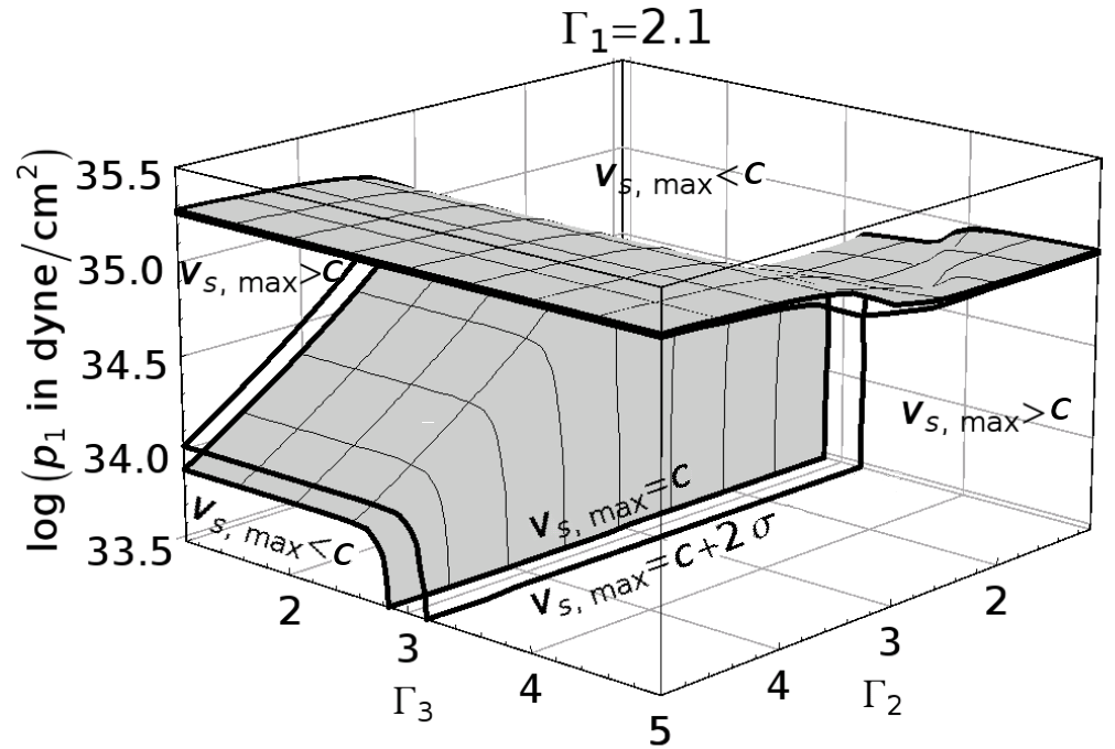
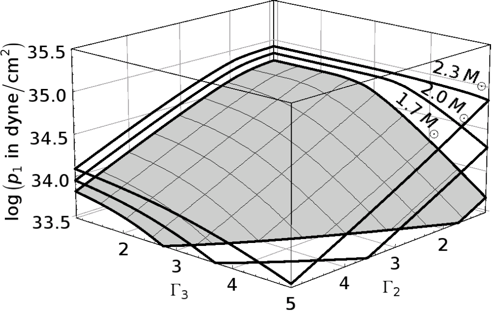
Figure 1: Left: Causality constraints are shown for a fixed value of $\Gamma_{1}$. For each EOS, the maximum speed of sound up to the central density of the maximum mass star is considered. The shaded surface separates the EOS parameter space into a region behind the surface allowed by causality, labeled $v_{s}<c$, and a region in which corresponding EOSs violate causality, labeled $v_{s}>c$. The second, outlined surface shows a weaker constraint to accommodate the expected error ($\sim 2$ standard deviations $\sigma$) in the speed of sound associated with a piecewise polytropic approximation to an EOS.
Right: Surfaces representing the set of parameters resulting in a constant maximum mass. A single observation of a massive neutron star constrains the equation of state to lie above the corresponding surface. The exponent $\Gamma_{1}$ is set to the least constraining value at each point (figures adopted from [1]).

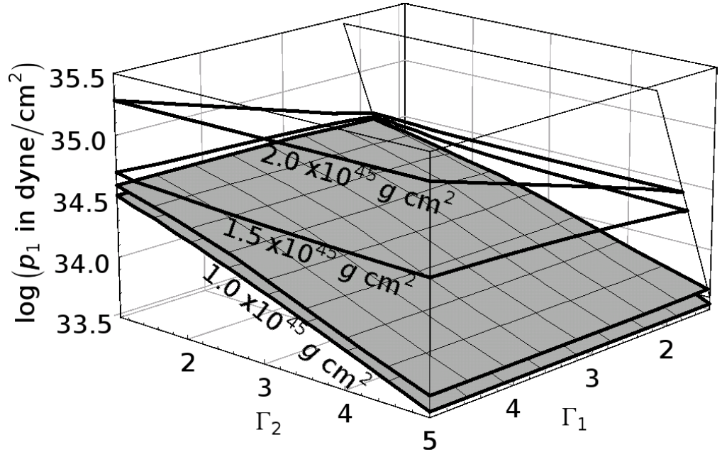
Figure 2: Left: Surfaces that represent the set of parameters that result in a star with a mass of 1.338 $M_{\odot}$ and a given moment of inertia $I$ (from possible near-future observations of PSR J0737-3039A). Observation of moment of inertia $I$ for a known mass $M$ constrains the equation of state to lie on the corresponding surface.
Right: Surfaces representing the set of parameters that result in a star with a mass of 1.4 $M_{\odot}$ and a fixed radius $R$. Measurement of the radius $R$ of a neutron star with known mass $M$ constrains the equation of state to lie on the corresponding surface. The wedge at the back right in both figures corresponds to incompatible values of $p_{1}$ and $\Gamma_{1}$ (figures adopted from [1]).

2.2 Initial candidate equations of state

Systematic variation of the EOS parameters also allows us to determine which properties significantly affect the gravitational radiation produced, and thus can be constrained with detection of sufficiently strong gravitational waves.

The models selected for this study use a variation of one EOS parameter in the neutron star core. We vary the core EOS by an overall pressure shift $p_{1}$ (specified at the fiducial density $\rho_{1}=10^{14.7}$ g cm^-3), while holding the adiabatic index in the core regions fixed at $\Gamma_{1}=\Gamma_{2}=\Gamma_{3}=3$. While only a subset of realistic EOS are well-approximated by a single core polytrope, reducing the EOS considered to this single-parameter family allows us to estimate parameter measurability with a reasonable number of simulations.

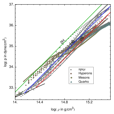
Figure 3: Initial choices of EOS for numerical evolution compared to the set of tabled EOS considered in [1]. Candidates are labelled in order of increasing softness: 2H, HB, 2B. Reproduced with permission from [56] ©(2009) by the American Physical Society.

After fixing the core adiabatic index, increasing the overall pressure scale $p_{1}$ produces a family of neutron stars with progressively increasing radius for a given mass; the choice of parameter $p_{1}$ is partly motivated by the observation of Lattimer and Prakash [3] that pressure at one to two times nuclear density is closely tied to neutron star radius, with $R\propto p_{1}^{1/4}$. The radius is less sensitive to variation of the adiabatic index in the neutron star core, for reasonable adiabatic indices [1], as suggested by Fig. 2.

Future work will incorporate additional variations of the EOS within the core. This could involve additional models of varying adiabatic index around a fixed $p_{1}$ (with $\Gamma_{1}=\Gamma_{2}=\Gamma_{3}$ in all core layers), as well as multiple piecewise-polytrope zones (with $\Gamma_{1}\neq\Gamma_{2}\neq\Gamma_{3}$) within the core or EOS parameters yielding neutron stars of the same mass $M$ and radius $R$ but different internal structure. Such work would yield insight into the relative size and correlation of effects on the orbital evolution due to the stellar radius and internal structure.

The first set of EOS were chosen to “bracket” the range of existing candidates, seen in Fig. 3. These models are HB with $p_{1}=10^{34.40}\,\text{dyn}\,\text{cm}^{-2}$, a standard EOS; 2H with $p_{1}=10^{34.90}\,\text{dyn}\,\text{cm}^{-2}$, a stiff EOS; 2B, with $p_{1}=10^{34.10}\,\text{dyn}\,\text{cm}^{-2}$, a soft EOS.

3 Numerical simulations

For each parameterized EOS considered, the late inspiral and merger of a binary neutron star system is simulated. The gravitational mass of each neutron star in the binary is fixed to $1.35M_{\odot}$, an average value for pulsars observed in binary systems [32, 33]. The significance of tidal effects in this configuration is expected to fairly represent tidal effects over the relatively narrow range of masses and mass ratios in astrophysical binary neutron star systems.

3.1 Initial data

Initial data is generated by constructing quasi-equilibrium sequences of irrotational neutron stars in a binary system, following the methods of [12, 21, 34, 35, 36, 37], using the Isenberg-Wilson-Mathews formulation [38, 39]. Since tidal spin-up in neutron star binaries is estimated to be negligible [5, 6], our initial data and quasi-equilibrium sequences are constructed assuming irrotational flow fields and neglecting the neutron star spin. The parameterized EOS of Eq. (1) is incorporated in the code to solve for initial data with a conformally flat spatial geometry coupled to the fluid equations of neutron star matter. The baryon number of each star is equal to that of a spherical isolated star with gravitational mass $M=1.35\,M_{\odot}$. The initial data for the full numerical simulation is taken from the quasi-equilibrium configuration at a separation such that approximately $3$ orbits remain until merger. Relevant quantities of the initial configurations for each parameterized EOS are presented in Tables 1, 2.

Table 1: Properties of initial candidate EOS. These range from the “softest” EOS at the top, which results in a prompt collapse to a black hole upon merger, to the “stiffest” at the bottom. Model HB is considered a typical EOS. The pressure $p_{1}$, which is the pressure at density $\rho_{1}=5\times 10^{14}\,\text{g}\,\text{cm}^{-3}$, determines the polytropic EOS for the neutron star core; all candidates have $\Gamma=3$. Radius $R$ and compactness $GM/c^{2}R$ are those of a single isolated spherical (TOV) star of gravitational mass $M=1.35\,M_{\odot}$, with radius measured in Schwarzschild coordinates. The maximum neutron star mass $M_{\text{max}}$ is given in the fifth column.

Model	$\log_{10}p_{1}\,[\mbox{dyn}\,\mbox{cm}^{-2}]$	$R\,[\mbox{km}]$	$GM/c^{2}R$	$M_{\text{max}}\,[M_{\odot}]$
2H	34.90	15.2	0.13	2.83
HB	34.40	11.6	0.17	2.12
2B	34.10	09.7	0.21	1.78

Table 2: Quantities of initial data sets for irrotational binary neutron stars. Each star has a baryon number $M_{0}$ equal to that of an isolated star with gravitational mass $M=1.35\,M_{\odot}$. The ADM mass $M_{\text{ADM}}$ of the initial slice includes the binding energy and $J$ is the total angular momentum of the initial slice.

Model	$\rho_{\text{max}}\,[\mbox{g}\,\mbox{cm}^{-3}]$	$M_{0}\,[M_{\odot}]$	$M_{\text{ADM}}\,[M_{\odot}]$	$cJ/(GM_{\text{ADM}}^{2})$	$\Omega/2\pi$ [Hz]
2H	$3.73196\times 10^{14}$	1.45488	2.67262	0.993319	324.704
HB	$8.27673\times 10^{14}$	1.49273	2.67290	0.995361	309.928
2B	$1.38300\times 10^{15}$	1.52509	2.67229	0.987681	321.170

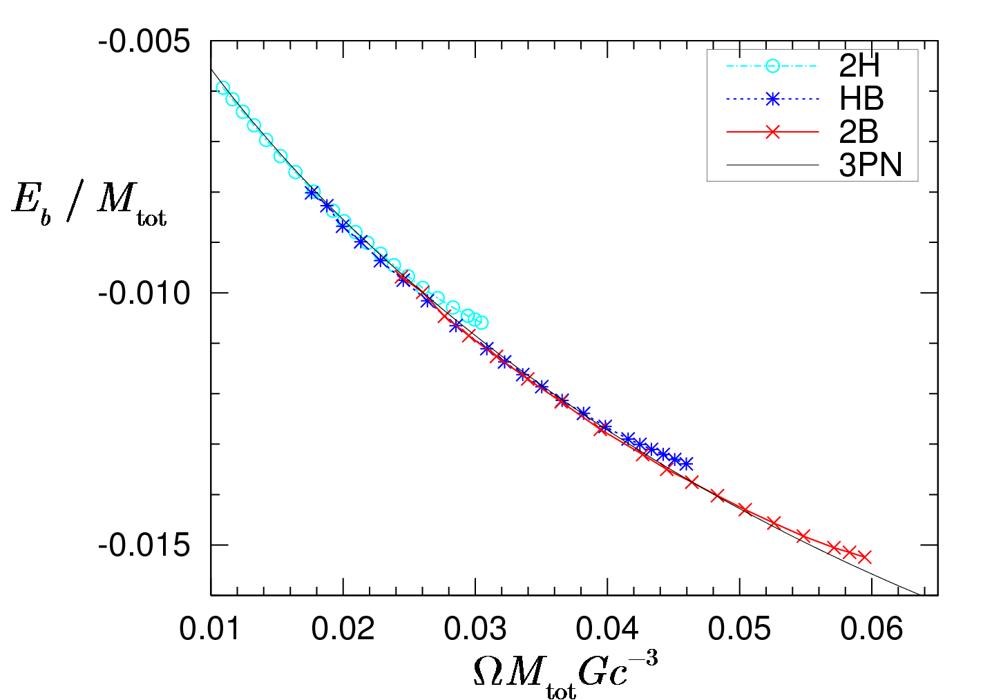
Figure 4: Binding energy $E_{\text{b}}:=M_{\text{ADM}}-M_{\rm{tot}}$ as a function of orbital frequency $\Omega$ for constant rest mass quasi-equilibrium sequences. The gravitational mass of each neutron star in isolation is $M=M_{\rm{tot}}/2=1.35\,M_{\odot}$. Departure from the point particle (3PN) curve occurs earlier for the stiffest EOS (candidate 2H – lowest compactness) and later for the softest EOS (candidate 2B – highest compactness).

3.2 Numerical evolution

The Einstein equations are solved using the Baumgarte-Shapiro-Shibata-Nakamura formulation [40, 41]. The conformal factor of the spatial metric is evolved following [42] and the resulting black hole spacetime is handled using the moving puncture method [43, 44]. The lapse and shift are evolved using a dynamical gauge condition as in [42], while the Einstein equations coupled to the fluid equations are solved using the numerical scheme also described in [42, 56].

During inspiral, the fluid evolution is essentially free of shocks, whence the cold parameterized EOS specified in Sec. 2 is used in the simulations. During merger, when shocks are developed, we include a hot EOS component with a thermal effective adiabatic index $\Gamma_{\rm eff}$, as described in [46]. Shock heating in the merger can increase the thermal energy up to $\sim 20$–30% of the total energy [17]. The merger and post-merger evolution is significantly affected by this hot component, since a collapse to a black hole may be delayed by the thermal pressure developed during and after merger.

Gravitational radiation is extracted both by spatially decomposing the metric perturbation about flat spacetime in the wave-zone with spin-2 weighted spherical harmonics and by calculating the outgoing part of the Weyl scalar $\Psi_{4}$. For equal mass neutron stars, such as those studied here, the quadrupole $(\ell=2,m=\pm 2)$ mode is much larger than any other mode, so we consider only this mode in this analysis. The waveforms output from the simulations are the cross and plus amplitudes $h_{+}c^{2}D/GM_{\text{tot}}$ and $h_{\times}c^{2}D/GM_{\text{tot}}$ of the quadrupole waveform, as would be measured at large distance $D\gg GM_{\text{tot}}/c^{2}$ along the $z$ axis perpendicular to the plane of the orbit, versus the retarded time $t_{\text{ret}}$. Here $M_{\text{tot}}$ is the sum of the two neutron star masses when they are far apart, $M_{\text{tot}}=2.7M_{\odot}$. The early part of the extracted waveforms, for $t_{\text{ret}}\mathrel{\raise 1.29167pt\hbox{$<$}\mkern-14.0mu\lower 2.58334pt\hbox{$\sim$}}0$, contains spurious radiation which is discarded in the data analysis.

Each simulation is typically performed for three grid resolutions. In the best-resolution case, the diameter of each neutron star is covered with 60 grid points. Convergence tests with different grid resolutions indicate that, with the best grid resolution, the time duration in the inspiral phase is underestimated by about 1 orbit. This is primarily due to the fact that angular momentum is spuriously lost by numerical dissipation. Thus, the inspiral gravitational waves include a phase error, and as a result, the amplitude of the spectrum for the inspiral phase is slightly underestimated. However, it is found that the waveforms and resulting power spectrum for the late inspiral and merger phases, which we are most interested in for the present work, depend weakly on the grid resolution.

4 Analysis of inspiral waveforms

From the quadrupole waveform data, we construct the complex quantity

$$h=h_{+}-ih_{\times}$$ (6)

The amplitude and phase of this quantity define the instantaneous amplitude $|h|$ and phase $\phi=\arg h$ of the waveform. The instantaneous frequency $f$ of the quadrupole waveform is then estimated by

$$f=\frac{1}{2\pi}\frac{\Delta\phi}{\Delta t}$$ (7)

The numerical data can be shifted in phase and time by adding a time shift $\tau$ to the time series points and multiplying the complex $h$ by $e^{i\phi}$ to shift the overall wave phase by $\phi$.

It is useful to define a reference time marking the end of the inspiral and onset of merger. A natural choice for the end of the inspiral portion, considering the behaviour of a PP inspiral waveform, is the time of the peak in the waveform amplitude $|h|$. However, the amplitude of the numerical waveforms oscillates over the course of an orbit. A moving average of the waveform amplitude over $0.5$ ms segments is used to average this oscillation; the end of the inspiral is then defined as the time at the end of the maximum amplitude interval. The resulting merger time $t_{\text{M}}$ will be marked by solid vertical lines in the plots to follow.

The numerical waveforms begin at different orbital frequencies. To align them for comparison, they are each matched in the early inspiral region to the same post-Newtonian point-particle (or PP) waveform.

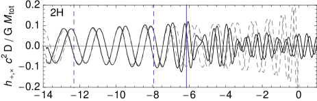
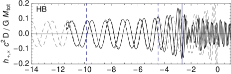
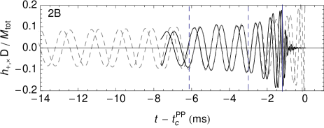
Figure 5: Solid lines show numerical waveforms, scaled by $c^{2}D/GM_{\text{tot}}$, and aligned in time and phase to the same point-particle post-Newtonian inspiral (dashed line), using a method described in [56]. The two dashed vertical bars indicate the portion of the waveform used for matching; the last vertical bar indicates the end of inspiral time $t_{\text{M}}$ for the numerical waveform. The top two simulations, 2H and HB, show the start of post-merger oscillations from a hypermassive neutron star remnant in the simulation. 2B shows quasinormal ringdown from a prompt collapse to a black hole following merger. Reproduced with permission from [56] ©(2009) by the American Physical Society.

4.1 Post-Newtonian point particle

Point-particle inspiral is not well-defined in full general relativity (GR), and one is left with the post-Newtonian point-particle (PP) approximation and fully general relativistic black-hole numerical solutions as natural substitutes. Fortunately, the Taylor T4 3.0/3.5 post-Newtonian specification, introduced in [47], agrees closely with numerical binary black hole waveforms for many cycles, up to and including the cycle before merger (see also [48]). This empirical agreement allows us to adopt the Taylor T4 waveform as an appropriate PP baseline waveform, compatible with full GR until the last cycles. Quasi-equilibrium sequences [Fig. 4] and time-frequency analysis [Fig. 6] show that the binary neutron star waveforms depart from this waveform $4$–$8$ cycles (200–560 $M_{\text{tot}}$) before the best-fit PP merger, due to finite size effects.

The TaylorT4 waveform is constructed by numerically integrating to obtain a gauge invariant post-Newtonian parameter related to the orbital frequency observed at infinity $\Omega$ [56]. The orbital frequency evolution $\Omega(t)$ and orbital phase evolution $\Phi(t)$ are computed to 3.5 post-Newtonian order following [47]. For the numerical integration, one needs to specify the constants of integration by fixing coalescence time $t_{\text{c}}^{\text{PP}}$ and the orbital phase at this time $\Phi(t_{\text{c}}^{\text{PP}})=\Phi_{\text{c}}^{\text{PP}}$. These two parameters uniquely specify the 3PN waveform for given particle masses. The amplitude of the ($l=2,m=\pm 2$) quadrupole waveform is then calculated to 3.0 post-Newtonian order as described in [49, 56].

To match the numerical data to the PP inspiral waveform, the two parameters, $t_{\text{c}}^{\text{PP}}$ and $\Phi_{\text{c}}^{\text{PP}}$ are varied and the best match is obtained [56], to fix a relative time shift and a relative phase shift. The masses of the point particles in the PP waveform are fixed to be the same as the neutron stars in the numerical simulations (the gravitational mass of isolated spherical neutron stars with the same number of baryons) and so masses are not varied in finding the best match. With a goal of signal analysis, we choose the time and phase shift by maximizing a correlation-based match between two waveforms. More details on the matching technique may be found in [56]. We note, however, that longer simulations are required to more precisely fix a post-Newtonian match.

4.2 Comparison of gravitational waveforms

Unlike the case of matching binary black hole simulations to point particle post-Newtonian[47, 48], the binary neutron star simulations show departure from point particle many cycles before the post-Newtonian merger time. Fig. 5 shows the four waveforms shifted so the best-match PP waveforms have the same $t_{\text{c}}^{\text{PP}}$ and $\phi_{\text{c}}^{\text{PP}}$. As the stiffness of the EOS and thus the radius of the neutron stars, increases, the end of inspiral for the binary neutron stars is shifted away from the end of inspiral for post-Newtonian point particle.

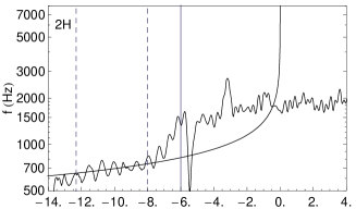
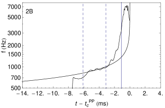
Figure 6: Time-frequency behavior, vertical line markings as previous figure. The departure from the point particle time-frequency relations, shown using a long-dashed line, occurs between $700$–$1000$ Hz depending on the EOS. In agreement with intuition and with Fig. 4, the departure occurs earlier for the stiffest and later for the softest EOS. Reproduced with permission from [56] ©(2009) by the American Physical Society.

This can also be seen by plotting the instantaneous frequency of the numerical simulation waveform with the same time shifts, as in Fig. 6, which also shows more clearly the difference in the post-merger oscillation frequencies of the hypermassive remnants, when present. The larger neutron star produced by the stiff EOS 2H has a lower oscillation frequency than that from the medium EOS HB. The remnant forms with a bar-mode oscillation stable over a longer period than the $\sim 10$ ms simulated. The signal from such a bar mode may be even stronger when the full lifetime is included. Information that can be extracted from the presence (or absence) and characteristics of a post-merger oscillation signal from the hyper-massive remnant would complement the information present in the late inspiral. Although such information could probe the equation of state at densities higher than those present in ordinary neutron stars, aspects of the physics neglected in this study will likely come into play. Such aspects may include finite temperature, magnetic field, neutrino cooling and other effects that need to be accurately modeled, thus complicating the parameter extraction. As previously noted, our simulations included a hot component in the equation of state, which strongly affects the post merger behavior (and prompt versus delayed collapse to a black hole in particular), but inclusion of other effects is a subject for future study.

4.3 Spectrum of gravitational waveforms

Given $h_{+}$ or $h_{\times}$, one can construct the discrete Fourier transforms (DFTs) $\tilde{h}_{+}$ or $\tilde{h}_{\times}$. Both polarizations yield the same DFT amplitude spectrum $|\tilde{h}|$, with phase shifted by $\pi/2$, if one neglects discretization, windowing, and numerical effects (including eccentricity). The amplitude spectrum $|\tilde{h}|$ is independent of phase and time shifts of the waveform.

The stationary phase approximation is valid for the post-Newtonian waveform up to frequencies of about 1500 Hz (with $\lesssim 10\%$ error), so is used to plot the amplitude of the point particle spectrum. In terms of an instantaneous frequency

$$f(t)=\frac{1}{2\pi}\frac{d\phi}{dt},$$ (8)

the Fourier transform of the waveform has the amplitude

$$|\tilde{h}|\simeq A(f)\left(\frac{df}{dt}\right)^{-1/2}.$$ (9)

For binaries comprised of equal mass companions, the gravitational radiation is dominated by quadrupole modes throughout the inspiral, so the analysis includes this mode only, as mentioned earlier. The wave phase $\phi$ is negligibly different from twice the orbital phase $2\Phi$ until the onset of merger at very high frequencies so we can use the relation

$$\frac{df}{dt}\simeq\frac{1}{\pi}\frac{d\Omega}{dt};$$ (10)

to write the amplitude of the Fourier transform entirely in terms of the functions $d\Omega/dt$ and the amplitude $A(f)=|h|$ of the polarization waveforms.

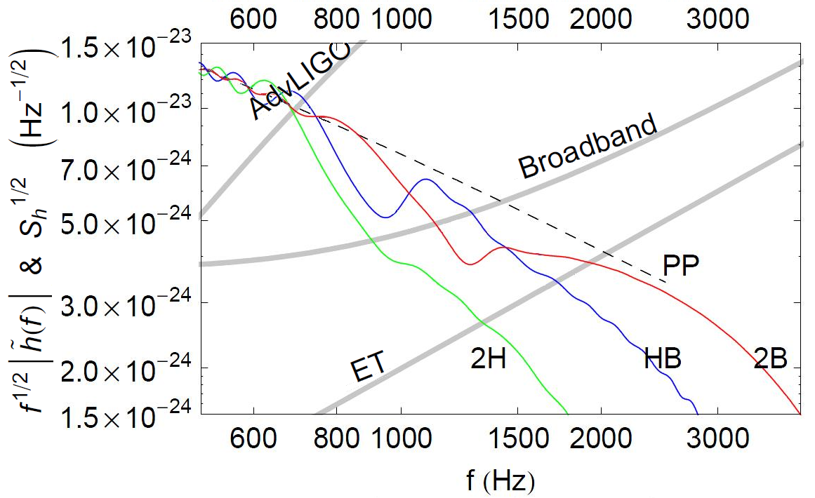
Figure 7: Colored curves show the DFT of full numerical inspiral waveforms, truncated and smoothly joined to best-match PP inspiral time series, at an effective distance $D_{\text{eff}}=100$ Mpc. The stationary-phase point particle is shown by a dashed line for reference. Thick grey lines represent the noise spectra for Advanced LIGO (labelled “AdvLIGO” for the standard configuration and “Broadband” for the broad-band configuration) and the Einstein Telescope (labelled “ET”). Reproduced with permission from [56] ©(2009) by the American Physical Society.

The translation of emitted waveforms into the strain amplitude measured at a detector involves transformations incorporating the effects of the emitting binary’s angle of inclination and sky location. These effects are absorbed into an effective distance $D_{\text{eff}}$, which is equal to the actual distance $D$ for a binary with optimal orientation and sky location, and is greater than the actual distance for a system that is not optimally oriented or located. The detector will detect a single polarization of the waveform, some combination of the plus and cross polarizations of the emitted waveform. The polarizations extracted from the simulation can be used as two estimates of the strain at the detector for a given numerically modelled source, which give very close results and are subsequently averaged.

To compare with noise curves in the usual units, the quantity $f^{1/2}|\tilde{h}(f)|$ is plotted, at a reference distance of $D_{\text{eff}}=100$ Mpc and rescaling from previously plotted numerical output $h(t)c^{2}D/GM_{\text{tot}}$ using $M_{\text{tot}}=2.7M_{\odot}$.

The full spectra of models 2H and HB, seen in Fig. 7, show peaks at post-merger oscillation frequencies. Waveforms of 2H and HB are truncated while the post-merger oscillation is ongoing; if the simulations were allowed to continue, these peaks would presumably grow further. The simulation of the softest candidate 2B, in contrast, promptly collapses to a black hole upon merger and has a short lived, and relatively small-amplitude, quasinormal mode ringdown.

Note that time-frequency plots like the ones in Fig. 6 showed that numerical waveforms follow the PP waveform at instantaneous frequencies of up to $700$–$1000$ Hz, depending on the EOS. The disagreement in the spectra in Fig. 7 from the PP stationary-phase approximation waveform at frequencies below this is primarily due to the finite starting time of the numerical waveforms. To estimate spectra from the full inspiral, we construct hybrid waveforms. The short-term numerical waveforms are smoothly merged on to long-inspiral PP-PN waveforms, using Hann windowing to smoothly turn on or turn off a signal. To construct hybrid waveforms, these windows are used to turn on the numerical waveform as the matched post-Newtonian is turned off, such that the sum of the two window functions is 1 over the matching range. Because, as mentioned earlier, the dependence on the cold EOS is less straightforward during the merger, due to unmodelled physics that become important at that time, we focus instead on the signal from the waveforms during the inspiral region only, turning off the waveforms after the end of inspiral, $t_{\text{M}}$.

5 Distinguishability and detectability

The question for neutron star astrophysics is whether these differences in the gravitational waveform will be measurable. We consider the possibility of detecting EOS effects with Advanced LIGO style detectors in varying configurations.

We use several detector configurations commonly considered for Advanced LIGO include tunings optimized for 1.4 $M_{\odot}$ NS-NS inspiral detection (“Standard”), for burst detection (“Broadband”), and for pulsars at 1150 Hz (“Narrowband”). The sensitivity is expressed in terms of the one-sided strain-equivalent amplitude spectral density $S_{h}(f)$ (which has units of $\mbox{Hz}^{-1/2}$) of the instrumental noise in Advanced LIGO. We also consider a provisional noise curve for the Einstein Telescope [51]. We consider only a single detector of each type, rather than a combination of detectors, for a preliminary estimate of detectability.

Given two signals $h_{1}$ and $h_{2}$, and a noise spectrum $S_{h}(f)$, we define the usual inner product [52]:

$$\langle h_{1}|h_{2}\rangle=4\mathop{\text{Re}}\nolimits\int_{0}^{\infty}\frac{\tilde{h}_{1}(f)\tilde{h}_{2}^{*}(f)}{S_{h}(f)}df.$$ (11)

This inner product yields a natural metric on a space of waveforms with distance between waveforms weighted by the inverse of the noise. The detector output $s$ is filtered against an expected waveform $h$ using $\langle s|h\rangle$. Then

$$\varrho=\frac{\langle s|h\rangle}{\sqrt{\langle h|h\rangle}}$$ (12)

is the optimal statistic to detect a waveform of known form $h$ in the signal $s$. If the detector output contains a particular waveform $h$ that is exactly matched by the template used, then the expectation value of $\varrho$ is the expected signal-to-noise ratio or SNR of that waveform:

$$\overline{\varrho}=\sqrt{\langle h|h\rangle}.$$ (13)

Given a signal $h_{1}$ to be used as a template, one can ask whether a known departure from this signal can be measured. Assuming the modified waveform $h_{2}$ is known, the expected SNR of $h_{2}-h_{1}$ is similarly

$$\overline{\varrho}_{\text{diff}}=\sqrt{\langle h_{2}-h_{1}|h_{2}-h_{1}\rangle}.$$ (14)

We consider the two signals to be marginally distinguishable [53] if the difference between the waveforms $h_{1}$ and $h_{2}$ has $\overline{\varrho}_{\text{diff}}\geq 1$.

To analyze the measurability of finite size effects, we consider differences between hybrid inspiral-only waveforms matched to point particle PN waveforms in the early inspiral. After the numerical waveforms have been matched to the same post-Newtonian point-particle inspiral, the signals will be aligned in time and phase. We then then compare the resulting waveforms to each other, and to a PN-only waveform, using different Advanced LIGO noise spectra. We report results in terms of the SNR measured by a single detector at an effective distance $D_{\text{eff}}=100$ Mpc. These results may be straightforwardly scaled to any distance in the wave zone, since $h$ and $\overline{\varrho}_{\text{diff}}$ are inversely proportional to the distance $D$.

Table 3: $\overline{\varrho}_{\text{diff}}$ in standard (NS-NS detection optimized) noise $\times\left(100\,\mbox{Mpc}/D_{\text{eff}}\right)$

Model	PP	2B	HB	2H
PP	0	0.32	0.55	0.69
2B		0	0.48	0.63
HB			0	0.60
2H				0

Table 4: $\overline{\varrho}_{\text{diff}}$ in broadband (burst-optimized) noise $\times\left(100\,\mbox{Mpc}/D_{\text{eff}}\right)$

Model	PP	2B	HB	2H
PP	0	1.86	2.67	2.89
2B		0	2.32	2.54
HB			0	2.37
2H				0

Table 5: $\overline{\varrho}_{\text{diff}}$ in narrowband $1150$ Hz noise $\times\left(100\,\mbox{Mpc}/D_{\text{eff}}\right)$

Model	PP	2B	HB	2H
PP	0	0.91	3.69	2.12
2B		0	2.92	1.45
HB			0	2.25
2H				0

The difference between waveforms due to finite size effects is not detectable in the NS-NS detection optimized configuration of Advanced LIGO for $\sim 100$ Mpc effective distances.

However, in both narrowband and broadband the differences can be significant, and waveforms are distinguishable from each other and from the PP waveform. Note that this implies that, even if the details of a NS-NS late inspiral signal are not known, the difference between it and a point particle waveform should be measurable. The quantity $\overline{\varrho}_{\text{diff}}$ between the observed waveform and a best fit point particle waveform, limited to differences at high frequency, may be useful in itself to constrain possible EOS independently of waveform details.

5.1 Parameter extraction

Since the early part of the inspiral is well described by a point particle post-Newtonian approximation, we will assume that EOS effects on the waveform impact the late inspiral only. For simplicity, we assume that orbital parameters, such as $M_{\text{tot}}$, mass ratio $\eta$, point particle post-Newtonian coalescence time $t_{\text{c}}^{\text{PP}}$, and phase shift $\phi_{\text{c}}^{\text{PP}}$, are determined from the observations of the earlier inspiral waveform, with sufficient accuracy that their measurement uncertainty will not affect the accuracy to which the late inspiral effects determine the EOS parameters. These measurements would be made by a broad-band instrument, in which the signal-to-noise ratio is expected to be high ($\sim 40$ at 100 Mpc) and measurement accuracy is expected to be good [52]. Inaccuracies in these measurement could lead to biases in the measured EOS. This will be an important aspect to assess when high-quality binary neutron star simulations with various masses become abundant.

With a one-parameter family of waveforms sampled, we can estimate the accuracy to which this parameter can be measured. There are also other EOS-related parameters which are not considered. In this first analysis we directly estimate the measurability of the EOS parameter $p_{1}$, ignoring variations of $\Gamma$ within the core. In the analysis of radius measurability, variations of the internal structures are respectively neglected. Expanding coverage of the EOS parameter space is underway. However, these initial parameter choices are expected to give the dominant contributions to finite size effects of the waveform. For example, the 1PN tidal effect estimates of [7, 54] predict $\sim$10% variation in the tidal terms contributing to binding energy and luminosity from changing internal structure—varying the apsidal constant—while keeping radius fixed.

We estimate errors in parameter estimation to first order in $1/\overline{\varrho}$ or, equivalently, in $\delta\theta^{A}$, using the Fisher matrix $\Gamma_{AB}=\langle\partial_{A}h|\partial_{B}h\rangle$ [52]. Its inverse, $(\Gamma^{-1})^{AB}$, yields

$$\overline{\delta\theta^{A}\delta\theta^{B}}=(\Gamma^{-1})^{AB}$$ (15)

so that the expected error in a given parameter $\theta^{A}$ is

$$\overline{\left(\delta\theta^{A}\right)^{2}}=(\Gamma^{-1})^{AA}$$ (16)

and the cross terms of the inverse Fisher matrix yield correlations between different parameters.

With a few simulations of varying parameter value, we estimate $\partial h/\partial{p_{1}}$ and $\partial h/\partial{R}$ from two of the sampled waveforms, $h_{1}$ and $h_{2}$. For a single parameter $\theta$ (which can be taken to be either $p_{1}$ or $R$), we have

$$\left.\frac{\partial h}{\partial{\theta}}\right|_{\theta=(\theta_{1}+\theta_{2})/2}\simeq\frac{h_{2}-h_{1}}{\theta_{2}-\theta_{1}}$$ (17)

where $h_{1}=h(\theta_{1})$ and $h_{2}=h(\theta_{2})$, and then, for our one-parameter family where we neglect correlations with other parameters, we have to first order

$$\overline{\left(\delta\theta\right)^{2}}\simeq\frac{(\theta_{2}-\theta_{1})^{2}}{\langle h_{2}-h_{1}|h_{2}-h_{1}\rangle}.$$ (18)

Using adjacent pairs of models to estimate waveform dependence at an average parameter value, we then find estimates of radius measurability as shown in Table 6 and $p_{1}$ measurability as shown in Table 7 for the burst-optimized noise and narrowband configurations.

Table 6: Measurability of radius $R$ (km) with broadband (burst-optimized) and narrowband (1150 Hz) configurations of Advanced LIGO, for a binary system at effective distance $100\,\mbox{Mpc}$. The values of $R$ here are midpoint values of the radii of candidates shown in Table 1. The error $\delta R$ (km) is estimated using Eqs. (14), (18) (with $\overline{\varrho}_{\text{diff}}$ taken from Tables 4, 5) and scales with effective distance as $\delta R\times\left(D_{\text{eff}}/100\,\mbox{Mpc}\right)$.

Configuration:	Broadband	Narrowband (1150 Hz)
$R=10.65$	$\pm 0.81$	$\pm 0.65$
$R=13.40$	$\pm 1.52$	$\pm 1.60$

Table 7: Measurability of pressure $p_{1}$ ($\mbox{dyn}\,\mbox{cm}^{-2}$) at the fiducial density $\rho_{1}=10^{14.7}$ g cm^-3, with broadband (burst-optimized) and narrowband (1150 Hz) configurations of Advanced LIGO, for a binary system at effective distance $100\,\mbox{Mpc}$. The values of $\mathrm{log}_{10}p_{1}$ here are midpoint values of $\mathrm{log}_{10}p_{1}$ from Table 1. The error $\delta\mathrm{log}_{10}p_{1}$ is estimated using Eqs. (14), (18) (with $\overline{\varrho}_{\text{diff}}$ taken from Tables 4, 5) and scales with effective distance as $\delta\mathrm{log}_{10}p_{1}\times\left(D_{\text{eff}}/100\,\mbox{Mpc}\right)$.

Model	Broadband	Narrowband (1150 Hz)
$\mathrm{log}_{10}p_{1}=34.25$	$\pm 0.13$	$\pm 0.10$
$\mathrm{log}_{10}p_{1}=34.65$	$\pm 0.21$	$\pm 0.22$

5.2 Sources of error

Many higher order but likely relevant effects have been neglected in this preliminary analysis. Tidal effects may measurably influence the orbital evolution before the start of the numerical simulations, as estimated in [7], slowly enough not to be seen over the few cycles of the waveform matched to PP in this analysis. In one sense this analysis is a worst-case scenario, as it assumes exact PP behavior before the numerical match. Earlier drift away from point particle dynamics would give larger differences between waveforms, and more sensitive radius measurement, but poses a challenge by requiring accurate numerical simulation over many cycles to verify EOS effects. Combining numerical estimation with PN analyses like those of [7, 8], and/or quasiequilibrium sequence information [Fig. 5] may clarify the transition between effectively PP and tidally influenced regimes.

Some residual eccentricity from initial data and finite numerical resolution is present in the waveforms themselves. The eccentricity error may be estimated by comparing the plus polarization to the cross polarization shifted by $\pi/2$ from the same numerical waveform. This results in $\overline{\varrho}_{\text{diff}}$ of $\sim 0.3$ for HB and 2H, rather than the expected quadrupole polarization cross-correlation of zero. The 2B waveform produces $\overline{\varrho}_{\text{diff}}\sim 0.05$ between polarizations.

We have only a coarsely sampled family of waveforms; estimates of $\partial h/\partial\theta$ are limited by this. Further, the length of the inspirals (see discussion on PN matching in [56]) limits precision in choosing the best match time. We can estimate these effects on current results by varying the match region considered; this changes $\overline{\varrho}_{\text{diff}}$ by up to $\sim 0.5$ at 100 Mpc in the broadband detector. The resolution from existing numerical simulations is comparable to the difference between parameters of some of the models. The estimated uncertainty in each $\overline{\varrho}_{\text{diff}}$ is smaller than (but comparable to) the $\overline{\varrho}_{\text{diff}}$ between candidates 2H, HB, 2B and PP.

Finally, we note that use of a Fisher matrix estimate of parameter measurement accuracy is fully valid only in high SNR limit of $\overline{\varrho}_{\text{diff}}>10$ [55], i.e., for distances $\lesssim 20$ Mpc in the broadband detector. The results do not take into account multiple detectors, nor multiple observations, nor parameter correlations. We conclude that, although these are of course first estimates, they should be better than order-of-magnitude. A full estimation of EOS parameter measurability will require more detailed analysis, with a larger set of inspiral simulations sampling a broader region of EOS parameter space, with mass ratios departing from unity, and with more orbits simulated before merger.

6 Summary

This is a first quantitative estimate of the measurability of the EOS of cold matter above nuclear density with gravitational wave detectors. Neutron stars of the same mass but different EOS and thus different radii will emit different gravitational waveforms during a late stage of binary inspiral. We calculated the signal strength of this difference in waveform using the sensitivity curves of commissioned and proposed gravitational wave detectors, and find that there is a measurably different signal from the inspirals of binary neutron stars with different EOS.

Although the standard noise configuration of Advanced LIGO is not sensitive to differences in the waveform from finite size effects, a broadband (burst-optimized) configuration or a narrowband detector configuration of Advanced LIGO can distinguish neutron star EOS from each other and from point particle inspiral, at an effective distance $\lesssim$ 100 Mpc. In addition, the provisional standard noise curve of the Einstein Telescope indicates the ability to resolve different EOS at roughly double that distance.

With broadband Advanced LIGO at frequencies between 500 and 1000 Hz, our first estimates show that the radius can be determined to an accuracy of $\delta R\sim 1\,\mbox{km}\times(100\,\mbox{Mpc}/D_{\text{eff}})$. Related first estimates show that such observations can constrain an EOS parameter parameter $p_{1}$, the pressure at a rest mass density $\rho_{1}=10^{14.7}$ g cm^-3, with an accuracy of $\delta p_{1}\sim 5\times 10^{33}\,\mbox{dyn}\,\mbox{cm}^{-2}\times(100\,\mbox{Mpc}/D_{\text{eff}})$. These estimates neglect correlations between the parameters and other details of internal structure, which are expected to give relatively small tidal effect corrections. Although these results are preliminary, they strongly motivate further work on gravitational wave constraints from binary neutron star inspirals. The accuracy of the estimates will be improved with numerical simulation of more orbits in the late inspiral and a wider exploration of the EOS parameter space.

7 Acknowledgments

It is a pleasure to thank the organizers of the 13th Conference on Recent Developments in Gravity (NEB- XIII) at Thessaloniki, for providing a very stimulating environment for research and discussion during the meeting. This work was supported in part by NSF grants PHY-0503366, PHY-0701817 and PHY-0200852, by NASA grant ATP03-0001-0027, and by JSPS Grants-in-Aid for Scientific Research(C) 20540275 and 19540263. CM thanks the Greek State Scholarships Foundation for support. Computation was done in part in the NAOJ and YITP systems.

References

References

- [1] Read J S, Lackey B, Friedman J L, and Owen B, astro-ph/0812.2163.
- [2] Read J S 2008 PhD Thesis, University of Wisconsin-Milwaukee
- [3] Lattimer J M and Prakash M, Ap. J. 550, 426 (2001), astro-ph/0002232.
- [4] Müller E, Eriguchi Y 1985 Ap. J. 152, 325-335.
- [5] Kochanek C S 1992 Ap.J. 398, 234.
- [6] Bildsten L and Cutler C Ap.J. 400, 175.
- [7] Flanagan É É and Hinderer T, Phys. Rev. D 77, 021502 (2008), 0709.1915.
- [8] Hinderer T, Lackey B and Read J S 2009 Work in preparation
- [9] Lai D and Wiseman A G, Phys. Rev. D 54, 3958 (1996), gr-qc/9609014.
- [10] Zhuge X, Centrella J M, and McMillan S L W, Phys. Rev. D 54, 7261 (1996), gr-qc/9610039.
- [11] Rasio F A and Shapiro S L, Classical and Quantum Gravity 16, 1 (1999), gr-qc/9902019.
- [12] Uryu K, Shibata M, and Eriguchi Y, Phys. Rev. D62, 104015 (2000), gr-qc/0007042.
- [13] Faber J A, Grandclément P, Rasio F A, and Taniguchi K, Physical Review Letters 89, 231102 (2002), astro-ph/0204397.
- [14] Faber J A, Grandclément P, and Rasio F A, Phys. Rev. D 69, 124036 (2004), gr-qc/0312097.
- [15] Bejger M, Gondek-Rosińska D, Gourgoulhon E, Haensel P, Taniguchi K, and Zdunik J L, Astronomy and Astrophysics 431, 297 (2005), astro-ph/0406234.
- [16] Gondek-Rosińska D, Bejger M, Bulik T, Gourgoulhon E, Haensel P, Limousin F, Taniguchi K, and Zdunik L, Advances in Space Research 39, 271 (2007).
- [17] Shibata M, Taniguchi K, and Uryū K, Phys. Rev. D 71, 084021 (2005), gr-qc/0503119.
- [18] Shibata M and Uryū K, Prog. Theor. Phys. 107, 265 (2003).
- [19] Oechslin R and Janka H-T, Phys. Rev. Lett. 99, 121102 (2007).
- [20] Hughes S A, Phys. Rev. D 66, 102001 (2002), gr-qc/0209012.
- [21] Taniguchi K and Gourgoulhon E, Phys. Rev. D 68, 124025 (2003), gr-qc/0309045.
- [22] Baumgarte T, Brady P R, Creighton J D E, Lehner L, Pretorius F, and Devoe R, Phys. Rev. D 77, 084009 (2008).
- [23] Shibata M, Phys. Rev. D 60, 104052 (1999), gr-qc/9908027.
- [24] Shibata M and Uryū K, Phys. Rev. D 61, 064001 (2000), gr-qc/9911058.
- [25] Shibata M and Taniguchi K, Phys. Rev. D 73, 064027 (2006), astro-ph/0603145.
- [26] Shibata M, Taniguchi K, and Uryū K, Phys. Rev. D 68, 084020 (2003), gr-qc/0310030.
- [27] Miller M, Gressman P, and Suen W-M, Phys. Rev. D 69, 064026 (2004), gr-qc/0312030.
- [28] Marronetti P, Duez M D, Shapiro S L, and Baumgarte T W, Phys. Rev. Lett. 92, 141101 (2004), gr-qc/0312036.
- [29] Liu Y T, Shapiro S L, Etienne Z B, and Taniguchi K, Phys. Rev. D 78, 024012 (2008), 0803.4193.
- [30] Yamamoto T, Shibata M, and Taniguchi K, Phys. Rev. D 78, 064054 (2008), 0806.4007.
- [31] Baiotti L, Giacomazzo B, and Rezzolla L (2008), gr-qc/0804.0594.
- [32] Thorsett S E and Chakrabarty D, Ap. J. 512, 288 (1999), astro-ph/9803260.
- [33] Stairs I H 2004, Science 304, 547.
- [34] Uryū K and Eriguchi Y 2000, Phys. Rev. D 61, 124023, gr-qc/9908059.
- [35] Bonazzola S, Gourgoulhon E, and Marck J-A 1999, Phys. Rev. Lett. 82, 892, gr-qc/9810072.
- [36] Gourgoulhon E, Grandclement P, Taniguchi K, Marck J-A, and Bonazzola S 2001, Phys. Rev. D D63, 064029, gr-qc/0007028.
- [37] Taniguchi K and Gourgoulhon E 2002, Phys. Rev. D 66, 104019, gr-qc/0207098.
- [38] Isenberg J A 2008, Int. J. Mod. Phys. D17, 265, gr-qc/0702113.
- [39] Wilson J R and Mathews G J 1995, Physical Review Letters 75, 4161.
- [40] Shibata M and Nakamura T, Phys. Rev. D 52, 5428 (1995).
- [41] Baumgarte T W and Shapiro S L 1999, Phys. Rev. D 59, 024007, gr-qc/9810065.
- [42] Shibata M and Taniguchi K 2008, Phys. Rev. D 77, 084015, 0711.1410.
- [43] Campanelli M, Lousto C O, Marronetti P, and Zlochower Y, Phys. Rev. Lett. 96, 111101 (2006), gr-qc/0511048.
- [44] Baker J G, Centrella J, Choi D-I, Koppitz M, and van Meter J 2006, Phys. Rev. Lett. 96, 111102, gr-qc/0511103.
- [45] Kurganov A and Tadmor E 2000, J. Comput. Phys. 160, 241.
- [46] Shibata M, Phys. Rev. D 67, 024033 (2003).
- [47] Boyle M, Brown D A, Kidder L E, Mroué A H, Pfeiffer H P, Scheel M A, Cook G B 2007, and Teukolsky S A, Phys. Rev. D 76, 124038, gr-qc/0710.0158.
- [48] Gopakumar A, Hannam M, Husa S, and Brügmann B 2007, Preprint 0712.3737.
- [49] Kidder L E, Phys. Rev. D 77, 044016 (2008).
- [50] Allen B, Anderson W G, Brady P R, Brown D A, and Creighton J D E 2005, Preprint gr-qc/0509116.
-
[51]
Van Den Broeck C 2008,
Tech. Rep. ,
(URL https://workarea.et-gw.eu/et/WG4-Astrophysics/base-sensitivity/). - [52] Cutler C and Flanagan É É, Phys. Rev. D 49, 2658 1994, gr-qc/9402014.
- [53] Lindblom L, Owen B J, and Brown D A 2008, 0809.3844.
- [54] Hinderer T 2008 Ap. J. 677, 1216 , Preprint 0711.2420.
- [55] Vallisneri M 2008 Phys. Rev. D 77, 042001
- [56] Read J S, Markakis C, Shibata M, Uryū K, Creighton J D E, and Friedman J L Phys. Rev. D 79, 124033, 2009 Preprint astro-ph/0901.3258, (URL http://prd.aps.org/abstract/PRD/v79/i12/e124033).