Crossed Andreev reflection and spin-resolved non-local electron transport

Abstract

The phenomenon of crossed Andreev reflection (CAR) is known to play a key role in non-local electron transport across three-terminal normal-superconducting-normal (NSN) devices. Here we review our general theory of non-local charge transport in three-terminal disordered ferromagnet-superconductor-ferromagnet (FSF) structures. We demonstrate that CAR is highly sensitive to electron spins and yields a rich variety of properties of non-local conductance which we describe non-perturbatively at arbitrary voltages, temperature, degree of disorder, spin-dependent interface transmissions and their polarizations. We demonstrate that magnetic effects have different implications: While strong exchange field suppresses disorder-induced electron interference in ferromagnetic electrodes, spin-sensitive electron scattering at SF interfaces can drive the total non-local conductance negative at sufficiently low energies. At higher energies magnetic effects become less important and the non-local resistance behaves similarly to the non-magnetic case. Our results can be applied to multi-terminal hybrid structures with normal, ferromagnetic and half-metallic electrodes and can be directly tested in future experiments.

0.1 Introduction

In hybrid NS structures quasiparticle current flowing in a normal metal is converted into that of Cooper pairs inside a superconductor. For quasiparticle energies above the superconducting gap $\varepsilon>\Delta$ this conversion is accompanied by electron-hole imbalance which relaxes deep inside a superconductor. At subgap energies $\varepsilon<\Delta$ the physical picture is entirely different. In this case quasiparticle-to-Cooper-pair current conversion is provided by the mechanism of Andreev reflection (AR) And : A quasiparticle enters the superconductor from the normal metal at a length of order of the superconducting coherence length $\xi_{S}$, forms a Cooper pair together with another quasiparticle, while a hole goes back into the normal metal. As a result, the net charge $2e$ is transferred through the NS interface which acquires non-zero subgap conductance down to $T=0$ BTK .

AR remains essentially a local effect provided there exists only one NS interface in the system or, else, if the distance between different NS interfaces greatly exceeds the superconducting coherence length $\xi$. If, however, the distance $L$ between two adjacent NS interfaces (i.e. the superconductor size) is smaller than (or comparable with) $\xi$, two additional non-local processes come into play (see Fig. 1). One such process corresponds to direct electron transfer between two N-metals through a superconductor. Another process is the so-called crossed Andreev reflection BF ; GF (CAR): An electron penetrating into the superconductor from the first N-terminal may form a Cooper pair together with another electron from the second N-terminal. In this case a hole will go into the second N-metal and AR becomes a non-local effect. This phenomenon of CAR enables direct experimental demonstration of entanglement between electrons in spatially separated N-electrodes and can strongly influence non-local transport of electrons in hybrid NSN systems.

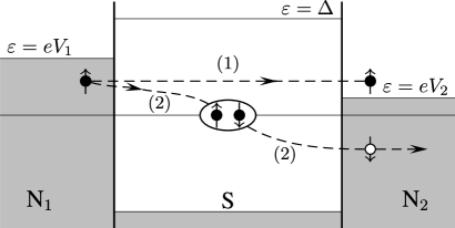
Figure 1: Two elementary processes contributing to non-local conductance of an NSN device: (1) direct electron transfer and (2) crossed Andreev reflection.

Non-local electron transport in the presence of CAR was recently investigated both experimentally Beckmann ; Teun ; Venkat ; Venkat2 ; Basel ; Deutscher ; Basel2 ; Beckmann2 and theoretically FFH ; KZ06 ; BG ; Belzig ; Duhot ; GZ07 ; LY ; KZ07 ; KZ07E ; KZ08 ; GZ09 ; GKZ ; Bergeret ; GZ10 (see also further references therein) demonstrating a rich variety of physical processes involved in the problem. It was shown FFH that in the lowest order in the interface transmission and at $T=0$ CAR contribution to cross-terminal conductance is exactly canceled by that from elastic electron cotunneling (EC), i.e. the non-local conductance vanishes in this limit. Taking into account higher order processes in barrier transmissions eliminates this feature and yields non-zero values of cross-conductance KZ06 .

Another interesting issue is the effect of disorder. It is well known that disorder enhances interference effects and, hence, can strongly modify local subgap conductance of NS interfaces in the low energy limit VZK ; HN ; Z . Non-local conductance of multi-terminal hybrid NSN structures in the presence of disorder was studied in a number of papers BG ; Belzig ; Duhot ; GZ07 ; GKZ ; Bergeret . A general quasiclassical theory was constructed by Golubev and the present authors GKZ . It was demonstrated that an interplay between CAR, quantum interference of electrons and non-local charge imbalance dominates the behavior of diffusive NSN systems being essential for quantitative interpretation of a number of experimental observations Venkat ; Basel ; Deutscher . In particular, strong enhancement of non-local spectral conductance was predicted at low energies due to quantum interference of electrons in disordered N-terminals. At the same time, non-local resistance $R_{12}$ remains smooth at small energies and, furthermore, was found to depend neither on parameters of NS interfaces nor on those of N-terminals. At higher temperatures $R_{12}$ was shown to exhibit a peak caused by the trade-off between charge imbalance and Andreev reflection.

Yet another interesting subject is an interplay between CAR and Coulomb interaction. The effect of electron-electron interactions on AR was investigated in a number of papers Z ; HHK ; GZ06 . Interactions should also affect CAR, e.g., by lifting the exact cancellation of EC and CAR contributions LY already in the lowest order in tunneling. A similar effect can occur in the presence of external ac fields GZ09 . A general theory of non-local transport in NSN systems with disorder and electron-electron interactions was very recently developed by Golubev and one of the present authors GZ10 direct relation between Coulomb effects and non-local shot noise. In the tunneling limit non-local differential conductance is found to have an S-like shape and can turn negative at non-zero bias. At high transmissions CAR turned out to be responsible both for positive noise cross-correlations and for Coulomb anti-blockade of non-local electron transport.

An important property of both AR and CAR is that these processes should be sensitive to magnetic properties of normal electrodes because these processes essentially depend on spins of scattered electrons. One possible way to demonstrate spin-resolved CAR is to use ferromagnets (F) instead of normal electrodes ferromagnet-superconductor-ferromagnet (FSF) structures. First experiments on such FSF structures Beckmann illustrated this point by demonstrating the dependence of non-local conductance on the polarization of ferromagnetic terminals. Hence, for better understanding of non-local effects in multi-terminal hybrid proximity structures it is necessary to construct a theory of spin-resolved non-local transport. In the case of ballistic systems in the lowest order order in tunneling this task was accomplished in FFH . Here we will generalize our quasiclassical approach KZ06 ; GKZ to explicitly focus on spin effects and construct a theory of non-local electron transport in both ballistic and diffusive NSN and FSF structures with spin-active interfaces beyond lowest order perturbation theory in their transmissions.

The structure of the paper is as follows. In Sec. 2 we will describe non-local spin-resolved electron transport in ballistic NSN structures with spin-active interfaces. In Sec. 3 we will further extend our formalism and evaluate both local and non-local conductances in SFS structures in the presence of disorder. Our main conclusions are briefly summarized in Sec. 4.

0.2 Spin-resolved transport in ballistic systems

Let us consider three-terminal NSN structure depicted in Fig. 2. We will assume that all three metallic electrodes are non-magnetic and ballistic, i.e. the electron elastic mean free path in each metal is larger than any other relevant size scale. In order to resolve spin-dependent effects we will assume that both NS interfaces are spin-active, i.e. we will distinguish “spin-up” and “spin-down” transmissions of the first ($D_{1\uparrow}$ and $D_{1\downarrow}$) and the second ($D_{2\uparrow}$ and $D_{2\downarrow}$) SN interface. All these four transmissions may take any value from zero to one. We also introduce the angle $\varphi$ between polarizations of two interfaces which can take any value between 0 and $2\pi$.

In what follows effective cross-sections of the two interfaces will be denoted respectively as $\mathcal{A}_{1}$ and $\mathcal{A}_{2}$. The distance between these interfaces $L$ as well as other geometric parameters are assumed to be much larger than $\sqrt{\mathcal{A}_{1,2}}$, i.e. effectively both contacts are metallic constrictions. In this case the voltage drops only across SN interfaces and not inside large metallic electrodes.

Figure 2: Schematics of our NSN device.

For convenience, we will set the electric potential of the S-electrode equal to zero, $V=0$. In the presence of bias voltages $V_{1}$ and $V_{2}$ applied to two normal electrodes (see Fig. 2) the currents $I_{1}$ and $I_{2}$ will flow through SN₁ and SN₂ interfaces. These currents can be evaluated with the aid of the quasiclassical formalism of nonequilibrium Green-Eilenberger-Keldysh functions BWBSZ $\hat{g}^{R,A,K}$ which we briefly specify below.

0.2.1 Quasiclassical equations

In the ballistic limit the corresponding Eilenberger equations take the form

$$\begin{split}\left[\varepsilon\hat{\tau}_{3}+eV(\bm{r},t)-\hat{\Delta}(\bm{r},t),\hat{g}^{R,A,K}(\bm{p}_{F},\varepsilon,\bm{r},t)\right]\\ +i\bm{v}_{F}\nabla\hat{g}^{R,A,K}(\bm{p}_{F},\varepsilon,\bm{r},t)=0,\end{split}$$ (1)

where $[\hat{a},\hat{b}]=\hat{a}\hat{b}-\hat{b}\hat{a}$, $\varepsilon$ is the quasiparticle energy, $\bm{p}_{F}=m\bm{v}_{F}$ is the electron Fermi momentum vector and $\hat{\tau}_{3}$ is the Pauli matrix in Nambu space. The functions $\hat{g}^{R,A,K}$ also obey the normalization conditions $(\hat{g}^{R})^{2}=(\hat{g}^{A})^{2}=1$ and $\hat{g}^{R}\hat{g}^{K}+\hat{g}^{K}\hat{g}^{A}=0$. Here and below the product of matrices is defined as time convolution.

Green functions $\hat{g}^{R,A,K}$ and $\hat{\Delta}$ are $4\times 4$ matrices in Nambu and spin spaces. In Nambu space they can be parameterized as

$$\hat{g}^{R,A,K}=\begin{pmatrix}g^{R,A,K}&f^{R,A,K}\\ \tilde{f}^{R,A,K}&\tilde{g}^{R,A,K}\\ \end{pmatrix},\quad\hat{\Delta}=\begin{pmatrix}0&\Delta i\sigma_{2}\\ \Delta^{*}i\sigma_{2}&0\\ \end{pmatrix},$$ (2)

where $g^{R,A,K}$, $f^{R,A,K}$, $\tilde{f}^{R,A,K}$, $\tilde{g}^{R,A,K}$ are $2\times 2$ matrices in the spin space, $\Delta$ is the BCS order parameter and $\sigma_{i}$ are Pauli matrices. For simplicity we will only consider the case of spin-singlet isotropic pairing in the superconducting electrode. The current density is related to the Keldysh function $\hat{g}^{K}$ according to the standard relation

$$\bm{j}(\bm{r},t)=\dfrac{eN_{0}}{8}\int d\varepsilon\left<\bm{v}_{F}\mathrm{Sp}[\hat{\tau}_{3}\hat{g}^{K}(\bm{p}_{F},\varepsilon,\bm{r},t)]\right>,$$ (3)

where $N_{0}=mp_{F}/2\pi^{2}$ is the density of state at the Fermi level and angular brackets $\left<...\right>$ denote averaging over the Fermi momentum.

0.2.2 Riccati parameterization

The above matrix Green-Keldysh functions can be conveniently parameterized by four Riccati amplitudes $\gamma^{R,A}$, $\tilde{\gamma}^{R,A}$ and two “distribution functions” $x^{K}$, $\tilde{x}^{K}$ (here and below we chose to follow the notations Eschrig00 ):

$$\hat{g}^{K}=2\hat{N}^{R}\begin{pmatrix}x^{K}-\gamma^{R}\tilde{x}^{K}\tilde{\gamma}^{A}&-\gamma^{R}\tilde{x}^{K}+x^{K}\gamma^{A}\\ -\tilde{\gamma}^{R}x^{K}+\tilde{x}^{K}\tilde{\gamma}^{A}&\tilde{x}^{K}-\tilde{\gamma}^{R}x^{K}\gamma^{A}\\ \end{pmatrix}\hat{N}^{A},$$ (4)

where functions $\gamma^{R,A}$ and $\tilde{\gamma}^{R,A}$ are Riccati amplitudes

$$\hat{g}^{R,A}=\pm\hat{N}^{R,A}\begin{pmatrix}1+\gamma^{R,A}\tilde{\gamma}^{R,A}&2\gamma^{R,A}\\ -2\tilde{\gamma}^{R,A}&-1-\tilde{\gamma}^{R,A}\gamma^{R,A}\\ \end{pmatrix}$$ (5)

and $\hat{N}^{R,A}$ are the following matrices

$$\hat{N}^{R,A}=\begin{pmatrix}(1-\gamma^{R,A}\tilde{\gamma}^{R,A})^{-1}&0\\ 0&(1-\tilde{\gamma}^{R,A}\gamma^{R,A})^{-1}\\ \end{pmatrix}.$$ (6)

With the aid of the above parameterization one can identically transform the quasiclassical equations (1) into the following set of effectively decoupled equations for Riccati amplitudes and distribution functions Eschrig00

$$\begin{split}i\bm{v}_{F}\nabla\gamma^{R,A}+[\varepsilon+eV(\bm{r},t)]\gamma^{R,A}+\gamma^{R,A}[\varepsilon-eV(\bm{r},t)]\\ =\gamma^{R,A}\Delta^{*}i\sigma_{2}\gamma^{R,A}-\Delta i\sigma_{2},\end{split}$$ (7)

$$\begin{split}i\bm{v}_{F}\nabla\tilde{\gamma}^{R,A}-[\varepsilon-eV(\bm{r},t)]\tilde{\gamma}^{R,A}-\tilde{\gamma}^{R,A}[\varepsilon+eV(\bm{r},t)]\\ =\tilde{\gamma}^{R,A}\Delta i\sigma_{2}\tilde{\gamma}^{R,A}-\Delta^{*}i\sigma_{2},\end{split}$$ (8)

$$\begin{split}i\bm{v}_{F}\nabla x^{K}+[\varepsilon+eV(\bm{r},t)]x^{K}-x^{K}[\varepsilon+eV(\bm{r},t)]\\ -\gamma^{R}\Delta^{*}i\sigma_{2}x^{K}-x^{K}\Delta i\sigma_{2}\tilde{\gamma}^{A}=0,\end{split}$$ (9)

$$\begin{split}i\bm{v}_{F}\nabla\tilde{x}^{K}-[\varepsilon-eV(\bm{r},t)]\tilde{x}^{K}+\tilde{x}^{K}[\varepsilon-eV(\bm{r},t)]\\ -\tilde{\gamma}^{R}\Delta i\sigma_{2}\tilde{x}^{K}-\tilde{x}^{K}\Delta^{*}i\sigma_{2}\gamma^{A}=0.\end{split}$$ (10)

Depending on the particular trajectory it is also convenient to introduce a “replica” of both Riccati amplitudes and distribution functions which – again following the notations Eschrig00 ; Zhao04 – will be denoted by capital letters $\Gamma$ and $X$. These “capital” Riccati amplitudes and distribution functions obey the same equations (7)-(10) with the replacement $\gamma\rightarrow\Gamma$ and $x\rightarrow X$. The distinction between different Riccati amplitudes and distribution functions will be made explicit below.

0.2.3 Boundary conditions

Figure 3: Riccati amplitudes for incoming and outgoing trajectories from the both sides of the interface.

Quasiclassical equations should be supplemented by appropriate boundary conditions at metallic interfaces. In the case of specularly reflecting spin-degenerate interfaces these conditions were derived by Zaitsev Zaitsev and later generalized to spin-active interfaces Millis88 , see also Eschrig09 for recent review on this subject.

Before specifying these conditions it is important to emphasize that the applicability of the Eilenberger quasiclassical formalism with appropriate boundary conditions to hybrid structures with two or more barriers is, in general, a non-trivial issue GZ02 ; OS . Electrons scattered at different barriers interfere and form bound states (resonances) which cannot be correctly described within the quasiclassical formalism employing Zaitsev boundary conditions or their direct generalization. Here we avoid this problem by choosing the appropriate geometry of our NSN device, see Fig. 2. In our system any relevant trajectory reaches each NS interface only once whereas the probability of multiple reflections at both interfaces is small in the parameter $\mathcal{A}_{1}\mathcal{A}_{2}/L^{4}\ll 1$. Hence, resonances formed by multiply reflected electron waves can be neglected, and our formalism remains adequate for the problem in question.

It will be convenient for us to formulate the boundary conditions directly in terms of Riccati amplitudes and the distribution functions. Let us consider the first NS interface and explicitly specify the relations between Riccati amplitudes and distribution functions for incoming and outgoing trajectories, see Fig. 3. The boundary conditions for $\Gamma_{1}^{R}$, $\tilde{\Gamma}_{1}^{A}$ and $X_{1}^{K}$ can be written in the form Zhao04

$$\Gamma_{1}^{R}=r_{1l}^{R}\gamma_{1}^{R}\underline{S}_{11}^{+}+t_{1l}^{R}\gamma_{1^{\prime}}^{R}{\underline{S}}_{11^{\prime}}^{+},$$ (11)

$$\tilde{\Gamma}_{1}^{A}=\underline{S}_{11}\tilde{\gamma}_{1}^{A}\tilde{r}_{1r}^{A}+{\underline{S}}_{11^{\prime}}\tilde{\gamma}_{1^{\prime}}^{A}\tilde{t}_{1r}^{A},$$ (12)

$$X_{1}^{K}=r_{1l}^{R}x_{1}^{K}\tilde{r}_{1r}^{A}+t_{1l}^{R}x_{1^{\prime}}^{K}\tilde{t}_{1r}^{A}-a_{1l}^{R}\tilde{x}_{1^{\prime}}^{K}\tilde{a}_{1r}^{A}.$$ (13)

Here we defined the transmission ($t$), reflection ($r$), and branch-conversion ($a$) amplitudes as:

$$r_{1l}^{R}=+[(\beta_{1^{\prime}1}^{R})^{-1}S_{11}^{+}-(\beta_{1^{\prime}1^{\prime}}^{R})^{-1}S_{11^{\prime}}^{+}]^{-1}(\beta_{1^{\prime}1}^{R})^{-1},$$ (14)

$$t_{1l}^{R}=-[(\beta_{1^{\prime}1}^{R})^{-1}S_{11}^{+}-(\beta_{1^{\prime}1^{\prime}}^{R})^{-1}S_{11^{\prime}}^{+}]^{-1}(\beta_{1^{\prime}1^{\prime}}^{R})^{-1},$$ (15)

$$\tilde{r}_{1r}^{A}=+(\beta_{1^{\prime}1}^{A})^{-1}[S_{11}(\beta_{1^{\prime}1}^{A})^{-1}-S_{11^{\prime}}(\beta_{1^{\prime}1^{\prime}}^{A})^{-1}]^{-1},$$ (16)

$$\tilde{t}_{1r}^{A}=-(\beta_{1^{\prime}1^{\prime}}^{A})^{-1}[S_{11}(\beta_{1^{\prime}1}^{A})^{-1}-S_{11^{\prime}}(\beta_{1^{\prime}1^{\prime}}^{A})^{-1}]^{-1},$$ (17)

$$a_{1l}^{R}=(\Gamma_{1}^{R}\underline{S}_{11}-S_{11}\gamma_{1}^{R})(\tilde{\beta}_{11^{\prime}}^{R})^{-1},$$ (18)

$$\tilde{a}_{1r}^{A}=(\tilde{\beta}_{11^{\prime}}^{A})^{-1}(\underline{S}_{11}^{+}\tilde{\Gamma}_{1}^{A}-\tilde{\gamma}_{1}^{A}S_{11}^{+}),$$ (19)

where

$$\beta_{ij}^{R}=S_{ij}^{+}-\gamma_{j}^{R}\underline{S}_{ij}^{+}\tilde{\gamma}_{i}^{R},\ \tilde{\beta}_{ij}^{R}=\underline{S}_{ji}-\tilde{\gamma}_{j}^{R}S_{ji}\gamma_{i}^{R},$$ (20)

$$\beta_{ij}^{A}=S_{ij}-\gamma_{i}^{A}\underline{S}_{ij}\tilde{\gamma}_{j}^{A},\ \tilde{\beta}_{ij}^{A}=\underline{S}_{ji}^{+}-\tilde{\gamma}_{i}^{A}S_{ji}^{+}\gamma_{j}^{A}.$$ (21)

Similarly, the boundary conditions for $\tilde{\Gamma}_{1}^{R}$, $\Gamma_{1}^{A}$, and $\tilde{X}_{1}^{K}$ take the form:

$$\tilde{\Gamma}_{1}^{R}=\tilde{r}_{1l}^{R}\tilde{\gamma}_{1}^{R}S_{11}+\tilde{t}_{1l}^{R}\tilde{\gamma}_{1^{\prime}}^{R}S_{1^{\prime}1},$$ (22)

$$\Gamma_{1}^{A}=S_{11}^{+}\gamma_{1}^{A}r_{1r}^{A}+S_{1^{\prime}1}^{+}\gamma_{1^{\prime}}^{A}t_{1r}^{A},$$ (23)

$$\tilde{X}_{1}^{K}=\tilde{r}_{1l}^{R}\tilde{x}_{1}^{K}r_{1r}^{A}+\tilde{t}_{1l}^{R}\tilde{x}_{1^{\prime}}^{K}t_{1r}^{A}-\tilde{a}_{1l}^{R}x_{1^{\prime}}^{K}a_{1r}^{A},$$ (24)

where

$$\tilde{r}_{1l}^{R}=+[(\tilde{\beta}_{1^{\prime}1}^{R})^{-1}\underline{S}_{11}-(\tilde{\beta}_{1^{\prime}1^{\prime}}^{R})^{-1}\underline{S}_{1^{\prime}1}]^{-1}(\tilde{\beta}_{1^{\prime}1}^{R})^{-1},$$ (25)

$$t_{1l}^{R}=-[(\tilde{\beta}_{1^{\prime}1}^{R})^{-1}\underline{S}_{11}-(\tilde{\beta}_{1^{\prime}1^{\prime}}^{R})^{-1}\underline{S}_{1^{\prime}1}]^{-1}(\tilde{\beta}_{1^{\prime}1^{\prime}}^{R})^{-1},$$ (26)

$$r_{1r}^{A}=+(\tilde{\beta}_{1^{\prime}1}^{A})^{-1}[\underline{S}_{11}^{+}(\tilde{\beta}_{1^{\prime}1}^{A})^{-1}-\underline{S}_{1^{\prime}1}^{+}(\tilde{\beta}_{1^{\prime}1^{\prime}}^{A})^{-1}]^{-1},$$ (27)

$$\tilde{t}_{1r}^{A}=-(\tilde{\beta}_{1^{\prime}1^{\prime}}^{A})^{-1}[\underline{S}_{11}^{+}(\tilde{\beta}_{1^{\prime}1}^{A})^{-1}-\underline{S}_{1^{\prime}1}^{+}(\tilde{\beta}_{1^{\prime}1^{\prime}}^{A})^{-1}]^{-1},$$ (28)

$$\tilde{a}_{1l}^{R}=(\tilde{\Gamma}_{1}^{R}S_{11}^{+}-\underline{S}_{11}^{+}\tilde{\gamma}_{1}^{R})(\beta_{11^{\prime}}^{R})^{-1},$$ (29)

$$a_{1r}^{A}=(\beta_{11^{\prime}}^{A})^{-1}(S_{11}\Gamma_{1}^{A}-\gamma_{1}^{A}\underline{S}_{11}).$$ (30)

Boundary conditions for $\Gamma_{1^{\prime}}^{R,A}$, $\tilde{\Gamma}_{1^{\prime}}^{R,A}$, $X^{K}_{1^{\prime}}$ and $\tilde{X}^{K}_{1^{\prime}}$ can be obtained from the above equations simply by replacing $1\leftrightarrow 1^{\prime}$.

The matrices $S_{11}$, $S_{11^{\prime}}$, $S_{1^{\prime}1}$, and $S_{1^{\prime}1^{\prime}}$ constitute the components of the $\mathcal{S}$-matrix describing electron scattering at the first interface:

$$\mathcal{S}=\begin{pmatrix}S_{11}&S_{11^{\prime}}\\ S_{1^{\prime}1}&S_{1^{\prime}1^{\prime}}\\ \end{pmatrix},\quad\mathcal{S}\mathcal{S}^{+}=1$$ (31)

Figure 4: Riccati amplitudes for incoming and outgoing trajectories for an NSN structure with two barriers. The arrows define quasiparticle momentum directions. We also indicate relevant Riccati amplitudes and distribution functions parameterizing the Green-Keldysh function for the corresponding trajectory.

In our three terminal geometry nonlocal conductance arises only from trajectories that cross both interfaces, as illustrated in Fig. 4. Accordingly, the above boundary conditions should be employed at both NS interfaces.

Finally, one needs to specify the asymptotic boundary conditions far from NS interfaces. Deep in metallic electrodes we have

$$\gamma_{1}^{R}=\tilde{\gamma}_{1}^{R}=\gamma_{1}^{A}=\tilde{\gamma}_{1}^{A}=0,$$ (32)

$$x_{1}^{K}=h_{0}(\varepsilon+eV_{1}),\quad\tilde{x}_{1}^{K}=-h_{0}(\varepsilon-eV_{1}),$$ (33)

$$\gamma_{2}^{R}=\tilde{\gamma}_{2}^{R}=\gamma_{2}^{A}=\tilde{\gamma}_{2}^{A}=0,$$ (34)

$$x_{2}^{K}=h_{0}(\varepsilon+eV_{2}),\quad\tilde{x}_{2}^{K}=-h_{0}(\varepsilon-eV_{2}),$$ (35)

where $h_{0}(\varepsilon)=\tanh(\varepsilon/2T)$ - equilibrium distribution function. In the bulk of superconducting electrode we have

$$\tilde{\gamma}_{1^{\prime}}^{R}=-a(\varepsilon)i\sigma_{2},\quad\gamma_{1^{\prime}}^{A}=a^{*}(\varepsilon)i\sigma_{2},$$ (36)

$$\tilde{x}_{1^{\prime}}^{K}=-[1-|a(\varepsilon)|^{2}]h_{0}(\varepsilon),$$ (37)

$$\gamma_{2^{\prime}}^{R}=a(\varepsilon)i\sigma_{2},\quad\tilde{\gamma}_{2^{\prime}}^{A}=-a^{*}(\varepsilon)i\sigma_{2},$$ (38)

$$x_{2^{\prime}}^{K}=[1-|a(\varepsilon)|^{2}]h_{0}(\varepsilon),$$ (39)

where we denoted $a(\varepsilon)=-(\varepsilon-\sqrt{\varepsilon^{2}-\Delta^{2}})/\Delta$.

0.2.4 Green functions

With the aid of the above equations and boundary conditions it is straightforward to evaluate the quasiclassical Green-Keldysh functions for our three-terminal device along any trajectory of interest. For instance, from the boundary conditions at the second interface we find

$$\Gamma_{2^{\prime}}^{R}=ia(\varepsilon)A_{2}\sigma_{2},$$ (40)

where $A_{2}=S_{2^{\prime}2^{\prime}}\sigma_{2}\underline{S}_{2^{\prime}2^{\prime}}^{+}\sigma_{2}$. Integrating Eq. (7) along the trajectory connecting both interfaces and using Eq. (40) as the initial condition we immediately evaluate the Riccati amplitude at the first interface:

$$\gamma_{1^{\prime}}^{R}=i\dfrac{aA_{2}+(aA_{2}\varepsilon+\Delta)Q}{1-(aA_{2}\Delta+\varepsilon)Q}\sigma_{2},$$ (41)

$$Q=\dfrac{\tanh\left[i\Omega L/v_{F}\right]}{\Omega},\quad\Omega=\sqrt{\varepsilon^{2}-\Delta^{2}}.$$ (42)

Employing the boundary conditions again we obtain

$$\Gamma_{1}^{R}=iS_{11^{\prime}}K_{21}^{-1}\left[aA_{2}+(aA_{2}\varepsilon+\Delta)Q\right]\sigma_{2}\underline{S}_{11^{\prime}}^{+},$$ (43)

$$\tilde{\Gamma}_{1}^{R}=-ia\underline{S}_{1^{\prime}1}^{+}\sigma_{2}S_{1^{\prime}1^{\prime}}K_{21}^{-1}\left[1-(aA_{2}\Delta+\varepsilon)Q\right]S_{1^{\prime}1^{\prime}}^{-1}S_{1^{\prime}1},$$ (44)

where

$$K_{ij}=(1-a^{2}A_{i}A_{j})-\left[\varepsilon(1+a^{2}A_{i}A_{j})+\Delta a(A_{i}+A_{j})\right]Q,$$ (45)

$$A_{1}=\sigma_{2}\underline{S}_{1^{\prime}1^{\prime}}^{+}\sigma_{2}S_{1^{\prime}1^{\prime}}.$$ (46)

We also note that the relation $(\Gamma^{R,A})^{+}=\tilde{\Gamma}^{A,R}$ and $(\gamma^{R,A})^{+}=\tilde{\gamma}^{A,R}$ makes it unnecessary (while redundant) to separately calculate the advanced Riccati amplitudes.

Let us now evaluate the distribution functions at both interfaces. With the aid of the boundary conditions at the second interface we obtain

$$X_{2^{\prime}}^{K}=S_{2^{\prime}2^{\prime}}S_{2^{\prime}2^{\prime}}^{+}\left(1-|a|^{2}\right)h_{0}(\varepsilon)+S_{2^{\prime}2}S_{2^{\prime}2}^{+}x_{2}^{K}\\ -|a|^{2}S_{2^{\prime}2^{\prime}}\sigma_{2}\underline{S}_{22^{\prime}}^{+}\underline{S}_{22^{\prime}}\sigma_{2}S_{2^{\prime}2^{\prime}}^{+}\tilde{x}_{2}^{K}.$$ (47)

Integrating Eq. (9) along the trajectory connecting both interfaces with initial condition for $X_{2^{\prime}}^{K}$, we arrive at the expression for $x_{1^{\prime}}^{K}$

$$x_{1^{\prime}}^{K}=\left[1-(aA_{2}\Delta+\varepsilon)Q\right]^{-1}X_{2^{\prime}}^{K}\\ \times(1-\tanh^{2}iL\Omega/v_{F})\left[1-(aA_{2}\Delta+\varepsilon)Q\right]^{+^{-1}}.$$ (48)

Then we can find distribution functions at the first interface. On the normal metal side of the interface we find

$$X_{1}^{K}=r_{1l}^{R}x_{1}^{K}r_{1l}^{R^{+}}+t_{1l}^{R}x_{1^{\prime}}^{K}t_{1l}^{R^{+}}+a_{1l}^{R}a_{1l}^{R^{+}}\left(1-|a|^{2}\right)h_{0}(\varepsilon)$$ (49)

where

$$\begin{split}r_{1l}^{R}=S_{11^{\prime}}K_{21}^{-1}\Bigl{[}(1-(aA_{2}\Delta+\varepsilon)Q)S_{1^{\prime}1^{\prime}}^{+}S_{1^{\prime}1}^{+^{-1}}\\ -a(aA_{2}+(aA_{2}\varepsilon+\Delta)Q)\sigma_{2}\underline{S}_{1^{\prime}1^{\prime}}^{+}\sigma_{2}S_{1^{\prime}1}^{+^{-1}}\Bigr{]},\end{split}$$ (50)

$$t_{1l}^{R}=S_{11^{\prime}}K_{21}^{-1}(1-(aA_{2}\Delta+\varepsilon)Q),$$ (51)

$$a_{1l}^{R}=iS_{11^{\prime}}K_{21}^{-1}(aA_{2}+(aA_{2}\varepsilon+\Delta)Q)\sigma_{2}\underline{S}_{1^{\prime}1^{\prime}}^{+}.$$ (52)

The corresponding expression for $\tilde{X}_{1}^{K}$ is obtained analogously. We get

$$\tilde{X}_{1}^{K}=\tilde{r}_{1l}^{R}\tilde{x}_{1}^{K}\tilde{r}_{1l}^{R^{+}}-\tilde{t}_{1l}^{R}\tilde{t}_{1l}^{R^{+}}\left(1-|a|^{2}\right)h_{0}(\varepsilon)-\tilde{a}_{1l}^{R}x_{1^{\prime}}^{K}\tilde{a}_{1l}^{R^{+}}.$$ (53)

where

$$\begin{split}\tilde{r}_{1l}^{R}=-\Bigl{[}\underline{S}_{1^{\prime}1}^{-1}\underline{S}_{1^{\prime}1^{\prime}}\sigma_{2}(1-(aA_{2}\Delta+\varepsilon)Q)\\ -\underline{S}_{1^{\prime}1}^{-1}\sigma_{2}S_{1^{\prime}1^{\prime}}a(aA_{2}+(aA_{2}\varepsilon+\Delta)Q)\Bigr{]}K_{12}^{-1}\sigma_{2}\underline{S}_{11^{\prime}}^{+},\end{split}$$ (54)

$$\tilde{t}_{1l}^{R}=\underline{S}_{1^{\prime}1}^{+}\underline{S}_{1^{\prime}1^{\prime}}^{+^{-1}}\sigma_{2}(1-(aA_{2}\Delta+\varepsilon)Q)K_{12}^{-1}\sigma_{2}\underline{S}_{1^{\prime}1^{\prime}}^{+},$$ (55)

$$\tilde{a}_{1l}^{R}=ia\underline{S}_{1^{\prime}1}^{+}\sigma_{2}S_{1^{\prime}1^{\prime}}K_{21}^{-1}(1-(aA_{2}\Delta+\varepsilon)Q).$$ (56)

Combining the above results for the Riccati amplitudes and the distribution functions we can easily evaluate the Keldysh Green function at the first interface. For instance, for the trajectory $1^{out}$ (see Fig. 4) we obtain

$$g^{K}_{1^{out}}=2(X_{1}^{K}-\Gamma_{1}^{R}\tilde{x}_{1}^{K}\Gamma_{1}^{R^{+}}),\quad\tilde{g}^{K}_{1^{out}}=2\tilde{x}_{1}^{K}.$$ (57)

The Keldysh Green function for the trajectory $1^{in}$ is evaluated analogously, and we get

$$g^{K}_{1^{in}}=2x_{1}^{K},\quad\tilde{g}^{K}_{1^{in}}=2(\tilde{X}_{1}^{K}-\tilde{\Gamma}_{1}^{R}x_{1}^{K}\tilde{\Gamma}_{1}^{R^{+}}).$$ (58)

0.2.5 Nonlocal conductance: General results

Now we are ready to evaluate the current $I_{1}$ across the first interface. This current takes the form:

$$I_{1}=I_{1}^{BTK}(V_{1})-\dfrac{G_{0}}{8e}\int d\varepsilon\operatorname{\mathrm{Sp}}(\hat{\tau}_{3}\hat{g}^{K}_{1^{out}}-\hat{\tau}_{3}\hat{g}^{K}_{1^{in}}),$$ (59)

where

$$G_{0}=\frac{8\gamma_{1}\gamma_{2}\mathcal{N}_{1}\mathcal{N}_{2}}{R_{q}p_{F}^{2}L^{2}}$$ (60)

is the normal state conductance of our device at fully transparent interfaces, $p_{F}\gamma_{1(2)}$ is normal to the first (second) interface component of the Fermi momentum for electrons propagating straight between the interfaces, $\mathcal{N}_{1,2}=p_{F}^{2}\mathcal{A}_{1,2}/4\pi$ define the number of conducting channels of the corresponding interface, $R_{q}=2\pi/e^{2}$ is the quantum resistance unit.

Here $I_{1}^{BTK}(V_{1})$ stands for the contribution to the current through the first interface coming from trajectories that never cross the second interface. This is just the standard BTK contribution BTK ; Zhao04 . The non-trivial contribution is represented by the last term in Eq. (59) which accounts for the presence of the second NS interface. We observe that this non-local contribution to the current is small as $\propto 1p_{F}^{2}L^{2}$. This term will be analyzed in details below.

The functions $\hat{g}^{K}_{1^{in}}$ and $\hat{g}^{K}_{1^{out}}$ are the Keldysh Green functions evaluated on the trajectories $1^{in}$ and $1^{out}$ respectively. Using the above expression for the Riccati amplitudes and the distribution functions we find

$$\operatorname{\mathrm{Sp}}(\hat{\tau}_{3}\hat{g}^{K}_{1^{out}}-\hat{\tau}_{3}\hat{g}^{K}_{1^{in}})=2\operatorname{\mathrm{Sp}}[r_{1l}^{R}r_{1l}^{R^{+}}-\tilde{\Gamma}_{1}^{R}\tilde{\Gamma}_{1}^{R^{+}}-1](h_{0}(\varepsilon+eV_{1})-h_{0}(\varepsilon))\\ -2\operatorname{\mathrm{Sp}}[\tilde{r}_{1l}^{R}\tilde{r}_{1l}^{R^{+}}-\Gamma_{1}^{R}\Gamma_{1}^{R^{+}}-1](h_{0}(\varepsilon-eV_{1})-h_{0}(\varepsilon))\\ +2(1-\tanh^{2}iL\Omega/v_{F})\operatorname{\mathrm{Sp}}[K_{21}^{-1}\{S_{2^{\prime}2}S_{2^{\prime}2}^{+}(h_{0}(\varepsilon+eV_{2})-h_{0}(\varepsilon))\\ +|a|^{2}S_{2^{\prime}2^{\prime}}\sigma_{2}\underline{S}_{22^{\prime}}^{+}\underline{S}_{22^{\prime}}\sigma_{2}S_{2^{\prime}2^{\prime}}^{+}(h_{0}(\varepsilon-eV_{2})-h_{0}(\varepsilon))\}K_{21}^{+^{-1}}\\ \times(S_{11^{\prime}}^{+}S_{11^{\prime}}-|a^{2}|S_{1^{\prime}1^{\prime}}^{+}\sigma_{2}\underline{S}_{1^{\prime}1}\underline{S}_{1^{\prime}1}^{+}\sigma_{2}S_{1^{\prime}1^{\prime}})],$$ (61)

where we explicitly used the fact that in equilibrium $\operatorname{\mathrm{Sp}}(\hat{\tau}_{3}\hat{g}^{K}_{1^{out}}-\hat{\tau}_{3}\hat{g}^{K}_{1^{in}})\equiv 0$. Substituting (61) into (59), we finally obtain

$$I_{1}=I_{1}^{BTK}(V_{1})+I_{11}(V_{1})+I_{12}(V_{2}).$$ (62)

The correction to the local BTK current (arising from trajectories crossing also the second NS interface) has the following form

$$I_{11}(V_{1})=-\dfrac{G_{0}}{4e}\int d\varepsilon\bigl{\{}\operatorname{\mathrm{Sp}}[r_{1l}^{R}r_{1l}^{R^{+}}-\tilde{\Gamma}_{1}^{R}\tilde{\Gamma}_{1}^{R^{+}}-1](h_{0}(\varepsilon+eV_{1})-h_{0}(\varepsilon))\\ -\operatorname{\mathrm{Sp}}[\tilde{r}_{1l}^{R}\tilde{r}_{1l}^{R^{+}}-\Gamma_{1}^{R}\Gamma_{1}^{R^{+}}-1](h_{0}(\varepsilon-eV_{1})-h_{0}(\varepsilon))\bigr{\}},$$ (63)

while for the cross-current we obtain

$$I_{12}(V_{2})=-\dfrac{G_{0}}{4e}\int d\varepsilon(1-\tanh^{2}iL\Omega/v_{F})\\ \times\operatorname{\mathrm{Sp}}[K_{21}^{-1}\{S_{2^{\prime}2}S_{2^{\prime}2}^{+}(h_{0}(\varepsilon+eV_{2})-h_{0}(\varepsilon))\\ +|a|^{2}S_{2^{\prime}2^{\prime}}\sigma_{2}\underline{S}_{22^{\prime}}^{+}\underline{S}_{22^{\prime}}\sigma_{2}S_{2^{\prime}2^{\prime}}^{+}(h_{0}(\varepsilon-eV_{2})-h_{0}(\varepsilon))\}K_{21}^{+^{-1}}\\ \times(S_{11^{\prime}}^{+}S_{11^{\prime}}-|a^{2}|S_{1^{\prime}1^{\prime}}^{+}\sigma_{2}\underline{S}_{1^{\prime}1}\underline{S}_{1^{\prime}1}^{+}\sigma_{2}S_{1^{\prime}1^{\prime}})].$$ (64)

Figure 5: Diagrams representing four different contributions to the cross-current $I_{12}$ (64). Solid (dotted) lines correspond to propagating electron-like (hole-like) excitations and $t_{21}=K_{21}^{-1}/\cosh(iL\Omega/v_{F})$.

Eqs. (62)-(64) fully determine the current across the first interface at arbitrary voltages, temperature and spin-dependent interface transmissions.

In right hand side of Eq. (64) we can distinguish four contributions with different products of $S$-matrices. Each of these terms corresponds to a certain sequence of elementary events, such as transmission, reflection, Andreev reflection and propagation between interfaces. Diagrammatic representation of these four terms is offered in Fig. 5. The amplitude of each of the processes is given by the product of the amplitudes of the corresponding elementary events. For instance, the amplitude of the process in Fig. 5c is $f=-iS_{11^{\prime}}t_{21}S_{2^{\prime}2^{\prime}}a\sigma_{2}\underline{S}_{22^{\prime}}^{+}$. In Eq.(64) this process is identified by the term $\operatorname{\mathrm{Sp}}(ff^{+})$ with the hole distribution function as a prefactor. It is straightforward to observe that the processes of Fig. 5a, 5b and 5d correspond to the other three terms in (64). We also note that the processes of Fig. 5a and 5d describe direct electron (hole) transport, while the processes of Fig. 5b and 5c correspond to the contribution of CAR.

Assuming that both interfaces possess inversion symmetry as well as reflection symmetry in the plane normal to the corresponding interface we can choose $\mathcal{S}$-matrices in the following form

$$S_{11}=S_{1^{\prime}1^{\prime}}=\underline{S}^{T}_{11}=\underline{S}^{T}_{1^{\prime}1^{\prime}}=U(\varphi)\begin{pmatrix}\sqrt{R_{1\uparrow}}e^{i\theta_{1}/2}&0\\ 0&\sqrt{R_{1\downarrow}}e^{-i\theta_{1}/2}\\ \end{pmatrix}U^{+}(\varphi),$$ (65)

$$S_{11^{\prime}}=S_{1^{\prime}1}=\underline{S}^{T}_{11^{\prime}}=\underline{S}^{T}_{1^{\prime}1}=U(\varphi)i\begin{pmatrix}\sqrt{D_{1\uparrow}}e^{i\theta_{1}/2}&0\\ 0&\sqrt{D_{1\downarrow}}e^{-i\theta_{1}/2}\\ \end{pmatrix}U^{+}(\varphi),$$ (66)

$$S_{22}=S_{2^{\prime}2^{\prime}}=\underline{S}_{22}=\underline{S}_{2^{\prime}2^{\prime}}=\begin{pmatrix}\sqrt{R_{2\uparrow}}e^{i\theta_{2}/2}&0\\ 0&\sqrt{R_{2\downarrow}}e^{-i\theta_{2}/2}\\ \end{pmatrix},$$ (67)

$$S_{22^{\prime}}=S_{2^{\prime}2}=\underline{S}_{22^{\prime}}=\underline{S}_{2^{\prime}2}=i\begin{pmatrix}\sqrt{D_{2\uparrow}}e^{i\theta_{2}/2}&0\\ 0&\sqrt{D_{2\downarrow}}e^{-i\theta_{2}/2}\\ \end{pmatrix}.$$ (68)

Here $R_{1(2)\uparrow(\downarrow)}=1-D_{1(2)\uparrow(\downarrow)}$ are the spin dependent reflection coefficients of both NS interfaces, $\theta_{1,2}$ are spin-mixing angles and $U(\varphi)$ is the rotation matrix in the spin space which depends on the angle $\varphi$ between polarizations of the two interfaces,

$$U(\varphi)=\exp(-i\varphi\sigma_{1}/2)=\begin{pmatrix}\cos(\varphi/2)&-i\sin(\varphi/2)\\ -i\sin(\varphi/2)&\cos(\varphi/2)\\ \end{pmatrix}.$$ (69)

In general spin current is not conserved in heterostructures with spin active interfaces. However single barrier with $S$-matrix (67)-(68) does not violate spin current conservation Zhao07 . It is easy to show that in our two barrier structure with interface $S$-matrices (65)-(68) spin current is conserved in the normal state for arbitrary barriers polarizations and in superconducting state for collinear barriers polarizations.

Substituting the above expressions for the $S$-matrices into Eqs. (63) and (64) we arrive at the final results for both $I_{11}(V_{1})$ and $I_{12}(V_{2})$ which will be specified further below.

0.2.6 Cross-current

First let us consider the cross-current $I_{12}(V_{2})$. From the above analysis we obtain

$$I_{12}(V_{2})=-\dfrac{G_{0}}{4e}\int d\varepsilon\left[\tanh\dfrac{\varepsilon+eV_{2}}{2T}-\tanh\dfrac{\varepsilon}{2T}\right]\dfrac{1-\tanh^{2}iL\Omega/v_{F}}{W(z_{1},z_{2},\varepsilon,\varphi)}\\ \times\Bigl{\{}\left[D_{1\downarrow}D_{2\downarrow}-|a|^{2}D_{1\uparrow}D_{2\downarrow}(R_{1\downarrow}+R_{2\uparrow})+|a|^{4}D_{1\downarrow}R_{1\uparrow}D_{2\downarrow}R_{2\uparrow}\right]|K(z_{1},z_{2},\varepsilon)|^{2}\tilde{c}\\ +\left[D_{1\uparrow}D_{2\uparrow}-|a|^{2}D_{1\downarrow}D_{2\uparrow}(R_{1\uparrow}+R_{2\downarrow})+|a|^{4}D_{1\uparrow}R_{1\downarrow}D_{2\uparrow}R_{2\downarrow}\right]|K(z_{1}^{*},z_{2}^{*},\varepsilon)|^{2}\tilde{c}\\ +\left[D_{1\uparrow}D_{2\downarrow}-|a|^{2}D_{1\downarrow}D_{2\downarrow}(R_{1\uparrow}+R_{2\uparrow})+|a|^{4}D_{1\uparrow}R_{1\downarrow}D_{2\downarrow}R_{2\uparrow}\right]|K(z_{1}^{*},z_{2},\varepsilon)|^{2}\tilde{s}\\ +\left[D_{1\downarrow}D_{2\uparrow}-|a|^{2}D_{1\uparrow}D_{2\uparrow}(R_{1\downarrow}+R_{2\downarrow})+|a|^{4}D_{1\downarrow}R_{1\uparrow}D_{2\uparrow}R_{2\downarrow}\right]|K(z_{1},z_{2}^{*},\varepsilon)|^{2}\tilde{s}\Bigr{\}},$$ (70)

where we define $\tilde{c}=\cos^{2}(\varphi/2)$, $\tilde{s}=\sin^{2}(\varphi/2)$,

$$K(z_{1},z_{2},\varepsilon)=(1-a^{2}z_{1}z_{2})-\left[\varepsilon(1+a^{2}z_{1}z_{2})+\Delta a(z_{1}+z_{2})\right]Q,$$ (71)

$$\begin{split}W(z_{1},z_{2},\varepsilon,\varphi)=|K(z_{1},z_{2},\varepsilon)&K(z_{1}^{*},z_{2}^{*},\varepsilon)\cos^{2}(\varphi/2)\\ +&K(z_{1}^{*},z_{2},\varepsilon)K(z_{1},z_{2}^{*},\varepsilon)\sin^{2}(\varphi/2)|^{2}\end{split}$$ (72)

and $z_{i}=\sqrt{R_{i\uparrow}R_{i\downarrow}}\exp(i\theta_{i})$ ( $i=1,2$).

Eq. (70) represents our central result. It fully determines the non-local spin-dependent current in our three-terminal ballistic NSN structure at arbitrary voltages, temperature, interface transmissions and polarizations.

Let us introduce the non-local differential conductance

$$G_{12}(V_{2})=-\dfrac{\partial I_{1}}{\partial V_{2}}=-\dfrac{\partial I_{12}(V_{2})}{\partial V_{2}}.$$ (73)

Before specifying this quantity further it is important to observe that in general the conductance $G_{12}(V_{2})$ is not an even function of the applied voltage $V_{2}$. This asymmetry arises due to formation of Andreev bound states in the vicinity of a spin-active interface Fogel00 ; Barash02 . It disappears provided the spin mixing angles $\theta_{1}$ and $\theta_{2}$ remain equal to $0$ or $\pi$.

In the normal state we have $I_{12}(V_{2})=-G_{N_{12}}V_{2}$, where

$$G_{N_{12}}=\dfrac{G_{0}}{2}\bigl{[}(D_{1\downarrow}D_{2\downarrow}+D_{1\uparrow}D_{2\uparrow})\cos^{2}(\varphi/2)\\ +(D_{1\uparrow}D_{2\downarrow}+D_{1\downarrow}D_{2\uparrow})\sin^{2}(\varphi/2)\bigr{]}.$$ (74)

Turning to the superconducting state, let us consider the limit of low temperatures and voltage $T,V_{2}\ll\Delta$. In this limit only subgap quasiparticles contribute to the cross-current and the differential conductance becomes voltage-independent, i.e. $I_{12}=-G_{12}V_{2}$, where

$$G_{12}=G_{0}(1-\tanh^{2}L\Delta/v_{F})\\ \times\Biggl{\{}\dfrac{D_{1\uparrow}D_{1\downarrow}D_{2\uparrow}D_{2\downarrow}}{|K(z_{1},z_{2},0)|^{2}\tilde{c}+|K(z_{1},z_{2}^{*},0)|^{2}\tilde{s}}\\ +(D_{1\uparrow}-D_{1\downarrow})(D_{2\uparrow}-D_{2\downarrow})\dfrac{|K(z_{1},z_{2},0)|^{2}\tilde{c}-|K(z_{1},z_{2}^{*},0)|^{2}\tilde{s}}{\left(|K(z_{1},z_{2},0)|^{2}\tilde{c}+|K(z_{1},z_{2}^{*},0)|^{2}\tilde{s}\right)^{2}}\Biggr{\}}.$$ (75)

where, as before, $\tilde{c}=\cos^{2}(\varphi/2)$ and $\tilde{s}=\sin^{2}(\varphi/2)$. In the case of spin-isotropic interfaces Eqs. (75) and (70) reduce to the results KZ06 .

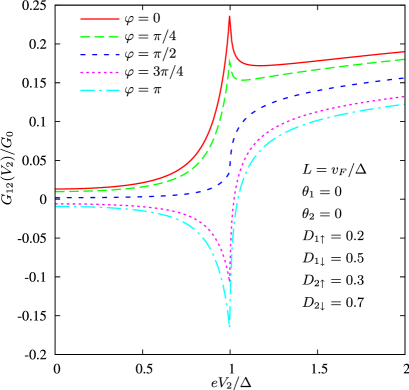
Figure 6: Zero temperature differential non-local conductance as a function of voltage at zero spin-mixing angles $\theta_{1,2}=0$.

Provided at least one of the interfaces is spin-isotropic, the conductance (75) is proportional to the product of all four transmissions $D_{1\uparrow}D_{1\downarrow}D_{2\uparrow}D_{2\downarrow}$, i.e. it differs from zero only due to processes involving scattering with both spin projections at both NS interfaces. As in the case of spin-isotropic interfaces KZ06 the value $G_{12}$ (75) gets strongly suppressed with increasing $L$, and at sufficiently high interface transmissions this dependence is in general non-exponential in $L$. In the spin-degenerate case for a given $L$ the non-local conductance reaches its maximum for reflectionless barriers $D_{1,2}=1$. In this case we arrive at a simple formula

$$G_{12}=G_{0}(1-\tanh^{2}L\Delta/v_{F}).$$ (76)

We observe that for small $L\ll v_{F}/\Delta$ the conductance $G_{12}$ identically coincides with its normal state value $G_{N_{12}}\equiv G_{0}$ at any temperature and voltage KZ06 . This result implies that CAR vanishes for fully open barriers. Actually this conclusion is general and applies not only for small but for any value of $L$, i.e. the result (76) is determined solely by the process of direct electron transfer between N-terminals for all $L$.

At the first sight, this result might appear counterintuitive since the behavior of ordinary (local) AR is just the opposite: It reaches its maximum at full barrier transmissions. The physics behind vanishing of CAR for perfectly trasparent NS interfaces is simple. One observes (cf. Fig. 1) that CAR inevitably implies the flow of Cooper pairs out of the contact area into the superconducting terminal. This flow is described by electron trajectories which end deep in the superconductor. On the other hand, it is obvious that CAR requires “mixing” of these trajectories with those going straight between two normal terminals. Provided there exists no normal electron reflection at both NS interfaces such mixing does not occur, CAR vanishes and the only remaining contribution to the non-local conductance is one from direct electron transfer between N-terminals.

This situation is illustrated by the diagrams in Fig. 5. It is obvious that in the case of non-reflecting NS interfaces only the process of Fig. 5a survives, whereas all other processes (Fig. 5b, 5c and 5d) vanish for reflectionless barriers with $R_{1(2)\uparrow(\downarrow)}=0$. The situation changes provided at least one of the transmissions is smaller than one. In this case scattering at SN interfaces mixes up trajectories connecting N₁ and N₂ terminals with ones going deep into and coming from the superconductor. As a result, all four processes depicted in Fig. 5 contribute to the cross-current and CAR contribution to $G_{12}$ does not vanish.

In the limit $|eV_{2}|,T\ll\Delta$ and at zero spin-mixing angles $\theta_{1,2}=0$ from Eq. (75) we obtain

$$G_{12}=G_{0}\dfrac{1-\tanh^{2}L\Delta/v_{F}}{|K(z_{1},z_{2},0)|^{2}}\bigl{\{}D_{1\uparrow}D_{1\downarrow}D_{2\uparrow}D_{2\downarrow}\\ +(D_{1\uparrow}-D_{1\downarrow})(D_{2\uparrow}-D_{2\downarrow})\cos\varphi\bigr{\}}.$$ (77)

In the lowest (first order) order in the transmissions of both interfaces and for collinear interface polarizations Eq. (77) reduces to the result by Falci et al. FFH provided we identify the tunneling density of states $N_{0}D_{1\uparrow}$, $N_{0}D_{1\downarrow}$, $N_{0}D_{2\uparrow}$, and $N_{0}D_{2\downarrow}$ with the corresponding spin-resolved densities of states in the ferromagnetic electrodes. For zero spin-mixing angles and low voltages the $L$-dependence of the nonlocal conductance $G_{12}$ reduces to the exponential form $G_{12}\propto\exp(-2L\Delta/v_{F})$ either in the limit of small transmissions or large $L\gg v_{F}/\Delta$.

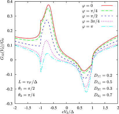
Figure 7: The same as in Fig. 6 for $\theta_{1}=\pi/2$, $\theta_{2}=\pi/4$.

At arbitrary voltages and temperatures the cross-current has a simple $\varphi$ dependence in the limit of zero spin mixing angles ($\theta_{1,2}=0$)

$$I_{12}(\varphi,V_{2})=I_{12}(\varphi=0,V_{2})\cos^{2}(\varphi/2)+I_{12}(\varphi=\pi,V_{2})\sin^{2}(\varphi/2),$$ (78)

i.e. in this limit at any $\varphi$ the nonlocal current is equal to a proper superposition of the two contributions corresponding to parallel ($\varphi=0$) and antiparallel ($\varphi=\pi$) interface polarizations. Some typical curves for the differential non-local conductance are presented in Fig. 6 at sufficiently high interface transmissions and zero spin mixing angles $\theta_{1,2}=0$.

Let us now turn to the limit of highly polarized interfaces which is accounted for by taking the limit of vanishing spin-up (or spin-down) transmission of each interface. In this limit our model describes an HSH structure, where H stands for fully spin-polarized half-metallic electrodes. In this case we obtain ($D_{1\uparrow}=D_{1}$, $D_{1\downarrow}=0$, $D_{2\uparrow}=D_{2}$, and $D_{2\downarrow}=0$)

$$I_{12}(V_{2})=-\dfrac{G_{0}}{4e}\int d\varepsilon\left[h_{0}(\varepsilon+eV_{2})-h_{0}(\varepsilon)\right]\dfrac{1-\tanh^{2}iL\Omega/v_{F}}{W(z_{1},z_{2},\varepsilon,\varphi)}D_{1}D_{2}\\ \times\Bigl{\{}\left[1+|a|^{4}\right]|K(z_{1}^{*},z_{2}^{*},\varepsilon)|^{2}\tilde{c}-2|a|^{2}|K(z_{1},z_{2}^{*},\varepsilon)|^{2}\tilde{s}\Bigr{\}}.$$ (79)

We observe that the nonlocal conductance has opposite signs for parallel ($\varphi=0$) and antiparallel ($\varphi=\pi$) interface polarizations. We also emphasize that, as it is also clear from Eq. (77), the cross-conductance $G_{12}$ of HSH structures – in contrast to that for NSN structures – does not vanish already in the lowest order in barrier transmissions $D_{1\uparrow}D_{2\uparrow}$.

In general the non-local conductance is very sensitive to particular values of the spin-mixing angles $\theta_{1}$ and $\theta_{2}$, as illustrated, e.g., in Fig. 7. Comparing the voltage dependencies of the nonlocal conductance evaluated for the same transmissions and presented in Figs.6 and 7, we observe that they can differ drastically at zero and non-zero values of $\theta_{1,2}$.

At low voltages and temperatures and at zero spin mixing angles the non-local conductance of HSH structures is determined by Eq. (77) with $D_{1\downarrow}=D_{2\downarrow}=0$. For fully open barriers (for ”spin-up” electrons) $D_{1\uparrow}=D_{2\uparrow}=1$ we obtain

$$G_{12}=G_{0}(1-\tanh^{2}L\Delta/v_{F})\cos\varphi.$$ (80)

Interestingly, for $\varphi=0$ this expression exactly coincides with that for fully open NSN structures, Eq. (76). At the same time for small $L$ the result (80) turns out to be 2 times bigger that the analogous expression in the normal case, i.e. for fully open HNH structures, cf. Eq. (74). This result can easily be interpreted in terms of diagrams in Fig. 5. We observe that – exactly as for the spin degenerate case – CAR diagrams of Fig. 5b,c vanish for reflectionless barriers, whereas diagrams of Fig. 5a,d describing direct electron transfer survive and both contribute to $G_{12}$. Thus, CAR vanishes identically also for fully open HSH structures. The factor of 2 difference with the normal case is due to the fact that the diagram of Fig. 5d vanishes in the normal limit.

0.2.7 Correction to BTK

Using the above formalism one can easily generalize the BTK result to the case of spin-polarized interfacesZhao04 . For the first interface we have

$$I_{1}^{BTK}(V_{1})=\dfrac{\mathcal{N}_{1}}{R_{q}e}\int d\varepsilon[h_{0}(\varepsilon+eV_{1})-h_{0}(\varepsilon)](1+|a|^{2})\\ \times\left<\dfrac{|v_{x_{1}}|}{v_{F}}\left(D_{1\uparrow}\dfrac{1-R_{1\downarrow}|a|^{2}}{|1-z_{1}a^{2}|^{2}}+D_{1\downarrow}\dfrac{1-R_{1\uparrow}|a|^{2}}{|1-z_{1}^{*}a^{2}|^{2}}\right)\right>.$$ (81)

Here transmission and reflection coefficients as well as the spin mixing angle depend on the direction of the Fermi momentum. In the spin-degenerate case the above expression reduces to the standard BTK result BTK .

Evaluating the nonlocal correction to the BTK current due to the presence of the second interface we arrive at a somewhat lengthy general expression

$$I_{11}(V_{1})=\dfrac{G_{0}}{2e}\int d\varepsilon(h_{0}(\varepsilon+eV_{1})-h_{0}(\varepsilon))\dfrac{1}{W(z_{1},z_{2},\varepsilon,\varphi)}\Bigl{\{}2W(z_{1},z_{2},\varepsilon,\varphi)\\ -R_{1\uparrow}\bigl{|}\tilde{c}K(z_{1}/R_{1\uparrow},z_{2},\varepsilon)K(z_{1}^{*},z_{2}^{*},\varepsilon)+\tilde{s}K(z_{1}/R_{1\uparrow},z_{2}^{*},\varepsilon)K(z_{1}^{*},z_{2},\varepsilon)\bigr{|}^{2}\\ -R_{1\downarrow}\bigl{|}\tilde{c}K(z_{1}^{*}/R_{1\downarrow},z_{2}^{*},\varepsilon)K(z_{1},z_{2},\varepsilon)+\tilde{s}K(z_{1}^{*}/R_{1\downarrow},z_{2},\varepsilon)K(z_{1},z_{2}^{*},\varepsilon)\bigr{|}^{2}\Bigr{\}}\\ +\dfrac{G_{0}}{4e}\int d\varepsilon(h_{0}(\varepsilon+eV_{1})-h_{0}(\varepsilon))\dfrac{D_{1\uparrow}D_{1\downarrow}}{W(z_{1},z_{2},\varepsilon,\varphi)}\Bigl{\{}\\ |a|^{2}\bigl{|}\tilde{c}K(0,z_{2},\varepsilon)K(z_{1}^{*},z_{2}^{*},\varepsilon)+\tilde{s}K(0,z_{2}^{*},\varepsilon)K(z_{1}^{*},z_{2},\varepsilon)\bigr{|}^{2}\\ +|a|^{2}\bigl{|}\tilde{c}K(0,z_{2}^{*},\varepsilon)K(z_{1},z_{2},\varepsilon)+\tilde{s}K(0,z_{2},\varepsilon)K(z_{1},z_{2}^{*},\varepsilon)\bigr{|}^{2}\\ +\dfrac{1}{|a|^{2}}\bigl{|}\tilde{c}K^{\prime}(z_{2}^{*},\varepsilon)K(z_{1},z_{2},\varepsilon)+\tilde{s}K^{\prime}(z_{2},\varepsilon)K(z_{1},z_{2}^{*},\varepsilon)\bigr{|}^{2}\\ +\dfrac{1}{|a|^{2}}\bigl{|}\tilde{c}K^{\prime}(z_{2},\varepsilon)K(z_{1}^{*},z_{2}^{*},\varepsilon)+\tilde{s}K^{\prime}(z_{2}^{*},\varepsilon)K(z_{1}^{*},z_{2},\varepsilon)\bigr{|}^{2}\Bigr{\}}\\ +\dfrac{G_{0}}{e}R_{2\uparrow}R_{2\downarrow}\sin^{2}(\theta_{2}/2)\tilde{s}\tilde{c}\\ \times\int d\varepsilon(h_{0}(\varepsilon+eV_{1})-h_{0}(\varepsilon))\dfrac{(1-\tanh^{2}iL\Omega/v_{F})^{2}}{W(z_{1},z_{2},\varepsilon,\varphi)}\\ \times\left[|a|^{2}(D^{2}_{1\uparrow}+D^{2}_{1\downarrow})-2|a|^{4}D_{1\uparrow}D_{1\downarrow}(R_{1\uparrow}+R_{1\downarrow})+|a|^{6}(D^{2}_{1\uparrow}R^{2}_{1\downarrow}+D^{2}_{1\downarrow}R^{2}_{1\uparrow})\right],$$ (82)

where $K^{\prime}(z_{2},\varepsilon)=\partial K(z_{1},z_{2},\varepsilon)/\partial z_{1}$. This expression gets significantly simplified in the limit of zero spin-mixing angles $\theta_{1,2}=0$ in which case we obtain

$$I_{11}(V_{1})=\dfrac{G_{0}}{2e}\int d\varepsilon(h_{0}(\varepsilon+eV_{1})-h_{0}(\varepsilon))\\ \times\Biggl{\{}2-R_{1\uparrow}\dfrac{|K(z_{1}/R_{1\uparrow},z_{2},\varepsilon)|^{2}}{|K(z_{1},z_{2},\varepsilon)|^{2}}-R_{1\downarrow}\dfrac{|K(z_{1}/R_{1\downarrow},z_{2},\varepsilon)|^{2}}{|K(z_{1},z_{2},\varepsilon)|^{2}}\\ +D_{1\uparrow}D_{1\downarrow}\dfrac{|a(\varepsilon)|^{2}|K(0,z_{2},\varepsilon)|^{2}+|K^{\prime}(z_{2},\varepsilon)|^{2}/|a(\varepsilon)|^{2}}{|K(z_{1},z_{2},\varepsilon)|^{2}}\Biggr{\}}.$$ (83)

In contrast to the expression for the cross-current $I_{12}$ (cf. Eq. (78)), in the limit of zero spin-mixing angles the correction $I_{11}$ to the BTK current does not depend on the angle $\varphi$ between the interface polarizations. In particular, at $|eV_{1}|,T\ll\Delta$ we have $I_{11}=G_{11}V_{1}$ where

$$G_{11}=G_{0}(D_{1\uparrow}+D_{1\downarrow})\dfrac{(1-z_{2}^{2})(1-\tanh^{2}L\Delta/v_{F})}{[1+z_{1}z_{2}+(z_{1}+z_{2})\tanh L\Delta/v_{F}]^{2}}\\ +G_{0}D_{1\uparrow}D_{1\downarrow}\dfrac{(1+z_{2}\tanh L\Delta/v_{F})^{2}+3(z_{2}+\tanh L\Delta/v_{F})^{2}}{[1+z_{1}z_{2}+(z_{1}+z_{2})\tanh L\Delta/v_{F}]^{2}}.$$ (84)

In the tunneling limit $D_{1\uparrow},D_{1\downarrow},D_{2\uparrow},D_{2\downarrow}\ll 1$ we reproduce the result of Ref. FFH

$$G_{11}=\dfrac{G_{0}}{4}(D_{1\uparrow}+D_{1\downarrow})(D_{2\uparrow}+D_{2\downarrow})\exp(-2L\Delta/v_{F}),$$ (85)

which turns out to hold at any value $\varphi$.

As compared to the BTK conductance the CAR correction (82) contains an extra small factor ${\cal A}_{2}/L^{2}$ and, hence, in many cases remains small and can be neglected. On the other hand, since CAR involves tunneling of one electron through each interface, for strongly asymmetric structures with $D_{1\uparrow},D_{1\downarrow}\ll 1$ and $D_{2\uparrow},D_{2\downarrow}\sim 1$ it can actually strongly exceed the BTK conductance. Indeed, for $D_{1\uparrow\downarrow}\ll 1$, $R_{2\uparrow}R_{2\downarrow}\ll 1$ and provided the spin mixing angle $\theta_{1}$ is not very close to $\pi$ from Eq. (82) we get

$$G_{11}=\dfrac{G_{0}(D_{1\uparrow}+D_{1\downarrow})}{\cosh(2L\Delta/v_{F})+\cos\theta_{1}\sinh(2L\Delta/v_{F})},$$ (86)

i.e. for

$$\frac{D_{1\uparrow}D_{1\downarrow}}{(D_{1\uparrow}+D_{1\downarrow})}<\frac{{\cal A}_{2}}{L^{2}}\exp(-2L\Delta/v_{F})$$

the contribution (86) may well exceed the BTK term $G_{1}^{BTK}\propto D_{1\uparrow}D_{1\downarrow}$. The existence of such a non-trivial regime further emphasizes the importance of the mechanism of non-local Andreev reflection in multi-terminal hybrid NSN structures.

0.3 Diffusive FSF structures

Let us now turn to the effect of disorder. In what follows we will consider a three-terminal diffusive FSF structure schematically shown in Fig. 8. Two ferromagnetic terminals F₁ and F₂ with resistances $r_{N_{1}}$ and $r_{N_{2}}$ and electric potentials $V_{1}$ and $V_{2}$ are connected to a superconducting electrode of length $L$ with normal state (Drude) resistance $r_{L}$ and electric potential $V=0$ via tunnel barriers. The magnitude of the exchange field $h_{1,2}=|\bm{h}_{1,2}|$ in both ferromagnets F₁ and F₂ is assumed to be much bigger than the superconducting order parameter $\Delta$ of the S-terminal and, on the other hand, much smaller that the Fermi energy, i.e. $\Delta\ll h_{1,2}\ll\epsilon_{F}$. The latter condition allows to perform the analysis of our FSF system within the quasiclassical formalism of Usadel equations for the Green-Keldysh matrix functions $G$ formulated below.

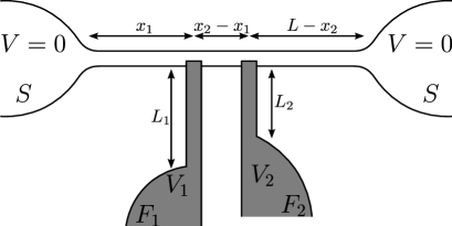
Figure 8: FSF structure under consideration.

0.3.1 Quasiclassical equations

In each of our metallic terminals the Usadel equations can be written in the form BWBSZ

$$iD\nabla(\check{G}\nabla\check{G})=[\check{\Omega}+eV,\check{G}],\quad\check{G}^{2}=1,$$ (87)

where $D$ is the diffusion constant, $V$ is the electric potential, $\check{G}$ and $\check{\Omega}$ are $8\times 8$ matrices in Keldysh-Nambu-spin space (denoted by check symbol)

$$\check{G}=\begin{pmatrix}\breve{G}^{R}&\breve{G}^{K}\\ 0&\breve{G}^{A}\\ \end{pmatrix},\quad\check{\Omega}=\begin{pmatrix}\breve{\Omega}^{R}&0\\ 0&\breve{\Omega}^{A}\\ \end{pmatrix},$$ (88)

$$\breve{\Omega}^{R}=\breve{\Omega}^{A}=\begin{pmatrix}\varepsilon-\hat{\bm{\sigma}}\bm{h}&\Delta\\ -\Delta^{*}&-\varepsilon+\hat{\bm{\sigma}}\bm{h}\\ \end{pmatrix},$$ (89)

$\varepsilon$ is the quasiparticle energy, $\Delta(T)$ is the superconducting order parameter which will be considered real in a superconductor and zero in both ferromagnets, $\bm{h}\equiv\bm{h}_{1(2)}$ in the first (second) ferromagnetic terminal, $\bm{h}\equiv 0$ outside these terminals and $\hat{\bm{\sigma}}=(\hat{\sigma}_{1},\hat{\sigma}_{2},\hat{\sigma}_{3})$ are Pauli matrices in spin space.

Retarded and advanced Green functions $\breve{G}^{R}$ and $\breve{G}^{A}$ have the following matrix structure

$$\breve{G}^{R,A}=\begin{pmatrix}\hat{G}^{R,A}&\hat{F}^{R,A}\\ -\hat{F}^{R,A}&-\hat{G}^{R,A}\\ \end{pmatrix}.$$ (90)

Here and below $2\times 2$ matrices in spin space are denoted by hat symbol.

Having obtained the expressions for the Green-Keldysh functions $\check{G}$ one can easily evaluate the current density $\bm{j}$ in our system with the aid of the standard relation

$$\bm{j}=-\frac{\sigma}{16e}\int\operatorname{\mathrm{Sp}}[\tau_{3}(\check{G}\nabla\check{G})^{K}]d\varepsilon,$$ (91)

where $\sigma$ is the Drude conductivity of the corresponding metal and $\tau_{3}$ is the Pauli matrix in Nambu space.

In what follows it will be convenient for us to employ the so-called Larkin-Ovchinnikov parameterization of the Keldysh Green function

$$\breve{G}^{K}=\breve{G}^{R}\breve{f}-\breve{f}\breve{G}^{A},\quad\breve{f}=\hat{f}_{L}+\tau_{3}\hat{f}_{T},$$ (92)

where the distribution functions $\hat{f}_{L}$ and $\hat{f}_{T}$ are $2\times 2$ matrices in the spin space.

For the sake of simplicity we will assume that magnetizations of both ferromagnets and the interfaces (see below) are collinear. Within this approximation the Green functions and the matrix $\check{\Omega}$ are diagonal in the spin space and the diffusion-like equations for the distribution function matrices $\hat{f}_{L}$ and $\hat{f}_{T}$ take the form

$$-D\nabla\left(\hat{D}^{T}(\bm{r},\varepsilon)\nabla\hat{f}_{T}(\bm{r},\varepsilon)\right)+2\hat{\Sigma}(\bm{r},\varepsilon)\hat{f}_{T}(\bm{r},\varepsilon)=0,$$ (93)

$$-D\nabla\left(\hat{D}^{L}(\bm{r},\varepsilon)\nabla\hat{f}_{L}(\bm{r},\varepsilon)\right)=0,$$ (94)

where

$$\hat{\Sigma}(\bm{r},\varepsilon)=-i\Delta\operatorname{\mathrm{Im}}\hat{F}^{R},$$ (95)

$$\hat{D}^{T}=\left(\operatorname{\mathrm{Re}}\hat{G}^{R}\right)^{2}+\left(\operatorname{\mathrm{Im}}\hat{F}^{R}\right)^{2},$$ (96)

$$\hat{D}^{L}=\left(\operatorname{\mathrm{Re}}\hat{G}^{R}\right)^{2}-\left(\operatorname{\mathrm{Re}}\hat{F}^{R}\right)^{2}.$$ (97)

The function $\hat{\Sigma}(\bm{r},\varepsilon)$ differs from zero only inside the superconductor. It accounts both for energy relaxation of quasiparticles and for their conversion to Cooper pairs due to Andreev reflection. The functions $\hat{D}^{T}$ and $\hat{D}^{L}$ acquire space and energy dependencies due to the presence of the superconducting wire and renormalize the diffusion coefficient $D$.

The solution of Eqs. (93)-(94) can be expressed in terms of the diffuson-like functions $\hat{\mathcal{D}}^{T}$ and $\hat{\mathcal{D}}^{L}$ which obey the following equations

$$-D\nabla\left[\hat{D}^{T}(\bm{r},\varepsilon)\nabla\hat{\mathcal{D}}^{T}(\bm{r},\bm{r}^{\prime},\varepsilon)\right]+2\hat{\Sigma}(\bm{r},\varepsilon)\hat{\mathcal{D}}^{T}(\bm{r},\bm{r}^{\prime},\varepsilon)=\delta(\bm{r}-\bm{r}^{\prime}),$$ (98)

$$-D\nabla\left[\hat{D}^{L}(\bm{r},\varepsilon)\nabla\hat{\mathcal{D}}^{L}(\bm{r},\bm{r}^{\prime},\varepsilon)\right]=\delta(\bm{r}-\bm{r}^{\prime}).$$ (99)

0.3.2 Boundary conditions

The solutions of Usadel equation (87) in each of the metals should be matched at FS-interfaces by means of appropriate boundary conditions which account for electron tunneling between these terminals. The form of these boundary conditions essentially depends on the adopted model describing electron scattering at FS-interfaces. As before, we stick to the model of the so-called spin-active interfaces which takes into account possibly different barrier transmissions for spin-up and spin-down electrons. Here we employ this model in the case of diffusive electrodes and also restrict our analysis to the case of tunnel barriers with channel transmissions much smaller than one. In this case the corresponding boundary conditions read Huertas02 ; Huertas09

$$\mathcal{A}\sigma_{+}\check{G}_{+}\partial_{x}\check{G}_{+}=\dfrac{G_{T}}{2}[\check{G}_{-},\check{G}_{+}]+\dfrac{G_{m}}{4}[\{\hat{\bm{\sigma}}\bm{m}\tau_{3},\check{G}_{-}\},\check{G}_{+}]+i\dfrac{G_{\varphi}}{2}[\hat{\bm{\sigma}}\bm{m}\tau_{3},\check{G}_{+}],$$ (100)

$$-\mathcal{A}\sigma_{-}\check{G}_{-}\partial_{x}\check{G}_{-}=\dfrac{G_{T}}{2}[\check{G}_{+},\check{G}_{-}]+\dfrac{G_{m}}{4}[\{\hat{\bm{\sigma}}\bm{m}\tau_{3},\check{G}_{+}\},\check{G}_{-}]+i\dfrac{G_{\varphi}}{2}[\hat{\bm{\sigma}}\bm{m}\tau_{3},\check{G}_{-}],$$ (101)

where $\check{G}_{-}$ and $\check{G}_{+}$ are the Green-Keldysh functions from the left ($x<0$) and from the right ($x>0$) side of the interface, $\mathcal{A}$ is the effective contact area, $\bm{m}$ is the unit vector in the direction of the interface magnetization, $\sigma_{\pm}$ are Drude conductivities of the left and right terminals and $G_{T}$ is the spin-independent part of the interface conductance. Along with $G_{T}$ there also exists the spin-sensitive contribution to the interface conductance which is accounted for by the $G_{m}$-term. The value $G_{m}$ equals to the difference between interface conductances for spin-up and spin-down conduction bands in the normal state. The $G_{\varphi}$-term arises due to different phase shifts acquired by scattered quasiparticles with opposite spin directions.

Employing the above boundary conditions we can establish the following linear relations between the distribution functions at both sides of the interface

$$\mathcal{A}\sigma_{+}\hat{D}_{+}^{T}\partial_{x}\hat{f}_{+T}=\mathcal{A}\sigma_{-}\hat{D}_{-}^{T}\partial_{x}\hat{f}_{-T}=\hat{g}_{T}(\hat{f}_{+T}-\hat{f}_{-T})+\hat{g}_{m}(\hat{f}_{+L}-\hat{f}_{-L}),$$ (102)

$$\mathcal{A}\sigma_{+}\hat{D}_{+}^{L}\partial_{x}\hat{f}_{+L}=\mathcal{A}\sigma_{-}\hat{D}_{-}^{L}\partial_{x}\hat{f}_{-L}=\hat{g}_{L}(\hat{f}_{+L}-\hat{f}_{-L})+\hat{g}_{m}(\hat{f}_{+T}-\hat{f}_{-T}),$$ (103)

where $\hat{g}_{T}$, $\hat{g}_{L}$, and $\hat{g}_{m}$ are matrix interface conductances which depend on the retarded and advanced Green functions at the interface

$$\hat{g}_{T}=G_{T}\left[\left(\operatorname{\mathrm{Re}}\hat{G}^{R}_{+}\right)\left(\operatorname{\mathrm{Re}}\hat{G}^{R}_{-}\right)+\left(\operatorname{\mathrm{Im}}\hat{F}^{R}_{+}\right)\left(\operatorname{\mathrm{Im}}\hat{F}^{R}_{-}\right)\right],$$ (104)

$$\hat{g}_{L}=G_{T}\left[\left(\operatorname{\mathrm{Re}}\hat{G}^{R}_{+}\right)\left(\operatorname{\mathrm{Re}}\hat{G}^{R}_{-}\right)-\left(\operatorname{\mathrm{Re}}\hat{F}^{R}_{+}\right)\left(\operatorname{\mathrm{Re}}\hat{F}^{R}_{-}\right)\right],$$ (105)

$$\hat{g}_{m}=G_{m}\hat{\bm{\sigma}}\bm{m}\left(\operatorname{\mathrm{Re}}\hat{G}^{R}_{+}\right)\left(\operatorname{\mathrm{Re}}\hat{G}^{R}_{-}\right).$$ (106)

Note that the above boundary conditions for the distribution functions do not contain the $G_{\varphi}$-term explicitly since this term in Eqs. (100)-(101) does not mix Green functions from both sides of the interface.

The current density (91) can then be expressed in terms of the distribution function $\hat{f}_{T}$ as

$$\bm{j}=-\frac{\sigma}{4e}\int\operatorname{\mathrm{Sp}}[\hat{D}^{T}\nabla\hat{f}_{T}]d\varepsilon.$$ (107)

0.3.3 Spectral conductances

Let us now employ the above formalism in order to evaluate electric currents in our FSF device. The current across the first (SF₁) interface can be written as

$$I_{1}=\dfrac{1}{e}\int g_{11}(\varepsilon)\left[f_{0}(\varepsilon+eV_{1})-f_{0}(\varepsilon)\right]d\varepsilon\\ -\dfrac{1}{e}\int g_{12}(\varepsilon)\left[f_{0}(\varepsilon+eV_{2})-f_{0}(\varepsilon)\right]d\varepsilon,$$ (108)

where $f_{0}(\varepsilon)=\tanh(\varepsilon/2T)$, $g_{11}$ and $g_{12}$ are local and nonlocal spectral electric conductances. Expression for the current across the second interface can be obtained from the above equation by interchanging the indices $1\leftrightarrow 2$. Solving Eqs. (93)-(94) with boundary conditions (102)-(103) we express both local and nonlocal conductances $\hat{g}_{ij}(\varepsilon)$ in terms of the interface conductances and the function $\hat{\mathcal{D}}$. The corresponding results read

$$\hat{g}_{11}(\varepsilon)=\bigl{(}\hat{R}_{2}^{T}\hat{\mathcal{M}}^{L}+\hat{R}_{2}^{T}\hat{R}_{2}^{L}\hat{R}_{1m}-\hat{R}_{1}^{L}\hat{R}_{2m}^{2}+\hat{R}_{12}^{T}\hat{R}_{12}^{L}\hat{R}_{2m}-\hat{R}_{1m}\hat{R}_{2m}^{2}\bigr{)}\hat{\mathcal{K}},$$ (109)

$$\hat{g}_{12}(\varepsilon)=\hat{g}_{21}(\varepsilon)=\bigl{(}\hat{R}_{12}^{T}\hat{\mathcal{M}}^{L}+\hat{R}_{2}^{T}\hat{R}_{12}^{L}\hat{R}_{1m}+\hat{R}_{12}^{L}\hat{R}_{1m}\hat{R}_{2m}+\hat{R}_{12}^{T}\hat{R}_{1}^{L}\hat{R}_{2m}\bigr{)}\hat{\mathcal{K}},$$ (110)

where we defined

$$\hat{\mathcal{M}}^{T,L}=\hat{R}_{1}^{T,L}\hat{R}_{2}^{T,L}-(\hat{R}_{12}^{T,L})^{2},$$ (111)

$$\hat{\mathcal{K}}^{-1}=\hat{\mathcal{M}}^{T}\hat{\mathcal{M}}^{L}+\hat{R}_{1m}^{2}\hat{R}_{2m}^{2}-\hat{R}_{2}^{T}\hat{R}_{2}^{L}\hat{R}_{1m}^{2}-2\hat{R}_{12}^{T}\hat{R}_{12}^{L}\hat{R}_{1m}\hat{R}_{2m}-\hat{R}_{1}^{T}\hat{R}_{1}^{L}\hat{R}_{2m}^{2}$$ (112)

and introduced the auxiliary resistance matrix

$$\hat{R}_{1}^{T}=\hat{g}_{1T}(\varepsilon)[\hat{g}_{1T}(\varepsilon)\hat{g}_{1L}(\varepsilon)-\hat{g}_{1m}^{2}(\varepsilon)]^{-1}\\ +\dfrac{D_{1}\hat{\mathcal{D}}_{1}^{T}(\bm{r}_{1},\bm{r}_{1},\varepsilon)}{\sigma_{1}}+\dfrac{D_{S}\hat{\mathcal{D}}_{S}^{T}(\bm{r}_{1},\bm{r}_{1},\varepsilon)}{\sigma_{S}},$$ (113)

The resistance matrices $\hat{R}_{2}^{T}$, $\hat{R}_{1}^{L}$ and $\hat{R}_{2}^{L}$ can be obtained by interchanging the indices $1\leftrightarrow 2$ and $T\leftrightarrow L$ in Eq. (113). The remaining resistance matrices $\hat{R}_{12}^{T,L}$ and $\hat{R}_{jm}$ are defined as

$$\hat{R}_{12}^{T,L}=\hat{R}_{21}^{T,L}=\dfrac{D_{S}\hat{\mathcal{D}}_{S}^{T,L}(\bm{r}_{1},\bm{r}_{2},\varepsilon)}{\sigma_{S}},$$ (114)

$$\hat{R}_{jm}=\hat{g}_{jm}(\varepsilon)[\hat{g}_{jT}(\varepsilon)\hat{g}_{jL}(\varepsilon)-\hat{g}_{jm}^{2}(\varepsilon)]^{-1},$$ (115)

where $j=1,2$. The spectral conductance $g_{ij}$ can be recovered from the matrix $\hat{g}_{ij}$ simply by summing up over the spin states

$$g_{ij}(\varepsilon)=\dfrac{1}{2}\operatorname{\mathrm{Sp}}\left[\hat{g}_{ij}(\varepsilon)\right].$$ (116)

It is worth pointing out that Eqs. (109), (110) defining respectively local and nonlocal spectral conductances are presented with excess accuracy. This is because the boundary conditions (100)-(101) employed here remain applicable only in the tunneling limit and for weak spin dependent scattering $|G_{m}|,|G_{\varphi}|\ll G_{T}$. Hence, strictly speaking only the lowest order terms in $G_{m_{1,2}}$ and $G_{\varphi_{1,2}}$ need to be kept in our final results.

In order to proceed it is necessary to evaluate the interface conductances as well as the matrix functions $\hat{\mathcal{D}}^{T,L}_{1,2,S}$. Restricting ourselves to the second order in the interface transmissions we obtain

$$\hat{g}_{1T}(\varepsilon)=G_{T_{1}}\hat{\nu}_{S}(\bm{r}_{1},\varepsilon)+G_{T_{1}}^{2}\dfrac{\Delta^{2}\theta(\Delta^{2}-\varepsilon^{2})}{\Delta^{2}-\varepsilon^{2}}\hat{U}_{1}(\varepsilon),$$ (117)

$$\hat{g}_{1L}(\varepsilon)=G_{T_{1}}\hat{\nu}_{S}(\bm{r}_{1},\varepsilon)-G_{T_{1}}^{2}\dfrac{\Delta^{2}\theta(\varepsilon^{2}-\Delta^{2})}{\varepsilon^{2}-\Delta^{2}}\hat{U}_{1}(\varepsilon),$$ (118)

$$\hat{g}_{1m}(\varepsilon)=G_{m_{1}}\hat{\nu}_{S}(\bm{r}_{1},\varepsilon)\hat{\bm{\sigma}}\bm{m}_{1},$$ (119)

and analogous expressions for the interface conductances of the second interface. The matrix function

$$\hat{U}_{1}(\varepsilon)=\dfrac{D_{1}}{2\sigma_{1}}\Bigl{\{}\operatorname{\mathrm{Re}}\left[\mathcal{C}_{1}(\bm{r}_{1},\bm{r}_{1},2h_{1}^{+})+\mathcal{C}_{1}(\bm{r}_{1},\bm{r}_{1},2h_{1}^{-})\right]\\ -\hat{\bm{\sigma}}\bm{m}_{1}\operatorname{\mathrm{Re}}\left[\mathcal{C}_{1}(\bm{r}_{1},\bm{r}_{1},2h_{1}^{+})-\mathcal{C}_{1}(\bm{r}_{1},\bm{r}_{1},2h_{1}^{-})\right]\Bigr{\}}$$ (120)

with $h_{1}^{\pm}=h_{1}\pm\varepsilon$ defines the correction due to the proximity effect in the normal metal.

Taking into account the first order corrections in the interface transmissions one can derive the density of states inside the superconductor in the following form

$$\hat{\nu}_{S}(\bm{r},\varepsilon)=\dfrac{|\varepsilon|\theta(\varepsilon^{2}-\Delta^{2})}{\sqrt{|\varepsilon^{2}-\Delta^{2}|}}+\dfrac{D_{S}}{\sigma_{S}}\dfrac{\Delta^{2}}{\Delta^{2}-\varepsilon^{2}}\sum_{i=1,2}\Biggl{[}G_{T_{i}}\operatorname{\mathrm{Re}}\mathcal{C}_{S}(\bm{r},\bm{r}_{i},2\omega^{R})\\ -\hat{\bm{\sigma}}\bm{m}_{i}G_{\varphi_{i}}\operatorname{\mathrm{Im}}\mathcal{C}_{S}(\bm{r},\bm{r}_{i},2\omega^{R})\Biggr{]},$$ (121)

where

$$\omega^{R}=\begin{cases}\sqrt{\varepsilon^{2}-\Delta^{2}},\quad&\varepsilon>\Delta,\\ i\sqrt{\Delta^{2}-\varepsilon^{2}},\quad&|\varepsilon|<\Delta,\\ -\sqrt{\varepsilon^{2}-\Delta^{2}},\quad&\varepsilon<\Delta,\end{cases}$$ (122)

and the Cooperon $\mathcal{C}_{j}(\bm{r},\bm{r}^{\prime},\varepsilon)$ represents the solution of the equation

$$\left(-D\nabla^{2}-i\varepsilon\right)\mathcal{C}(\bm{r},\bm{r}^{\prime},\varepsilon)=\delta(\bm{r}-\bm{r}^{\prime})$$ (123)

in the normal metal leads ($j=1,2$) and the superconductor ($j=S$). In the quasi-one-dimensional geometry the corresponding solutions take the form

$$\mathcal{C}_{j}(x_{j},x_{j},\varepsilon)=\dfrac{\tanh\left(k_{j}L_{j}\right)}{S_{j}D_{j}k_{j}},\quad j=1,2,$$ (124)

$$\mathcal{C}_{S}(x,x^{\prime},\varepsilon)=\dfrac{\sinh[k_{S}(L-x^{\prime})]\sinh k_{S}x}{k_{S}S_{S}D_{S}\sinh(k_{S}L)},\quad x^{\prime}>x,$$ (125)

where $S_{S,1,2}$ are the wire cross sections and $k_{1,2,S}=\sqrt{-i\varepsilon/D_{1,2,S}}$.

Substituting Eq. (121) into Eqs. (117) and (118) and comparing the terms $\propto G_{T_{1}}^{2}$ we observe that the tunneling correction to the density of states dominates over the terms proportional to $\hat{U}_{1}$ which contain an extra small factor $\sqrt{\Delta/h}\ll 1$. Hence, the latter terms in Eqs. (117) and (118) can be safely neglected. In addition, in Eq. (121) we also neglect small tunneling corrections to the superconducting density of states at energies exceeding the superconducting gap $\Delta$. Within this approximation the density of states inside the superconducting wire becomes spin-independent $\hat{\nu}_{S}(\bm{r},\varepsilon)=\hat{\sigma}_{0}\nu_{S}(\bm{r},\varepsilon)$. It can then be written as

$$\nu_{S}(\bm{r},\varepsilon)=\dfrac{|\varepsilon|}{\sqrt{|\varepsilon^{2}-\Delta^{2}|}}\theta(\varepsilon^{2}-\Delta^{2})\\ +\dfrac{D_{S}}{\sigma_{S}}\dfrac{\Delta^{2}\theta(\Delta^{2}-\varepsilon^{2})}{\Delta^{2}-\varepsilon^{2}}\sum\limits_{i=1,2}G_{T_{i}}\operatorname{\mathrm{Re}}\mathcal{C}_{S}(\bm{r},\bm{r}_{i},2\omega^{R}).$$ (126)

Accordingly, the interface conductances take the form

$$\hat{g}_{1T}(\varepsilon)=\hat{g}_{1L}(\varepsilon)=G_{T_{1}}\nu_{S}(\bm{r}_{1},\varepsilon),$$ (127)

$$\hat{g}_{1m}(\varepsilon)=G_{m_{1}}\nu_{S}(\bm{r}_{1},\varepsilon)\hat{\bm{\sigma}}\bm{m}_{1}.$$ (128)

Let us emphasize again that within our approximation the $G_{\varphi}$-term does not enter into expressions for the interface conductances (127)-(128) and, hence, does not appear in the final expressions for the conductances $g_{ij}(\varepsilon)$.

In the limit of strong exchange fields $h_{1,2}\gg\Delta$ and small interface transmissions considered here the proximity effect in the ferromagnets remains weak and can be neglected. Hence, the functions $\hat{\mathcal{D}}^{T,L}_{1}(\bm{r}_{1},\bm{r}_{1},\varepsilon)$ and $\hat{\mathcal{D}}^{T,L}_{2}(\bm{r}_{2},\bm{r}_{2},\varepsilon)$ can be approximated by their normal state values

$$\hat{\mathcal{D}}^{T,L}_{1}(\bm{r}_{1},\bm{r}_{1},\varepsilon)=\sigma_{1}r_{N_{1}}\hat{1}/D_{1},$$ (129)

$$\hat{\mathcal{D}}^{T,L}_{2}(\bm{r}_{2},\bm{r}_{2},\varepsilon)=\sigma_{2}r_{N_{2}}\hat{1}/D_{2},$$ (130)

$$r_{N_{j}}=L_{j}/(\sigma_{j}S_{j}),\quad j=1,2,$$ (131)

where $r_{N_{1}}$ and $r_{N_{2}}$ are the normal state resistances of ferromagnetic terminals. In the the superconducting region an effective expansion parameter is $G_{T_{1,2}}r_{\xi_{S}}(\varepsilon)$, where $r_{\xi_{S}}(\varepsilon)=\xi_{S}(\varepsilon)/(\sigma_{S}S_{S})$ is the Drude resistance of the superconducting wire segment of length $\xi_{S}(\varepsilon)=\sqrt{D_{S}/2|\omega^{R}|}$ and $\omega^{R}$ is the function of $\varepsilon$ according to Eq. (122). In the limit

$$G_{T_{1,2}}r_{\xi_{S}}(\varepsilon)\ll 1,$$ (132)

which is typically well satisfied for realistic system parameters, it suffices to evaluate the function $\hat{\mathcal{D}}^{T}_{S}(x,x^{\prime},\varepsilon)$ for impenetrable interfaces. In this case we find

$$\hat{\mathcal{D}}_{S}^{T}(x,x^{\prime},\varepsilon)=\begin{cases}\dfrac{\Delta^{2}-\varepsilon^{2}}{\Delta^{2}}\mathcal{C}_{S}(x,x^{\prime},2\omega^{R}),&|\varepsilon|<\Delta,\\ \dfrac{\varepsilon^{2}-\Delta^{2}}{\varepsilon^{2}}\mathcal{C}_{S}(x,x^{\prime},0),&|\varepsilon|>\Delta.\end{cases}$$ (133)

We note that special care should be taken while calculating $\mathcal{D}^{L}_{S}(x,x^{\prime},\varepsilon)$ at subgap energies, since the coefficient $D^{L}$ in Eq. (94) tends to zero deep inside the superconductor. Accordingly, the function $\mathcal{D}^{L}_{S}(x,x^{\prime},\varepsilon)$ becomes singular in this case. Nevertheless, the combinations $\hat{R}_{j}^{L}(\mathcal{M}^{L})^{-1}$ and $\hat{R}_{12}^{L}(\mathcal{M}^{L})^{-1}$ remain finite also in this limit. At subgap energies we obtain

$$\hat{R}_{1}^{L}(\hat{\mathcal{M}}^{L})^{-1}=\hat{R}_{2}^{L}(\hat{\mathcal{M}}^{L})^{-1}=\hat{R}_{12}^{L}(\hat{\mathcal{M}}^{L})^{-1}\\ =\dfrac{1}{r_{N_{1}}+r_{N_{2}}+\dfrac{2\kappa e^{d/\xi_{S}(\varepsilon)}}{r_{\xi_{S}}(\varepsilon)G_{T_{1}}G_{T_{2}}}},$$ (134)

where $\kappa=1-\varepsilon^{2}/\Delta^{2}$ and $d=|x_{2}-x_{1}|$ is the distance between two FS contacts. Substituting the above relations into Eq. (110) we arrive at the final result for the non-local spectral conductance of our device at subgap energies ($|\varepsilon|<\Delta$)

$$g_{12}(\varepsilon)=g_{21}(\varepsilon)=\dfrac{\kappa r_{\xi_{S}}(\varepsilon)\exp[-d/\xi_{S}(\varepsilon)]}{2[r_{N_{1}}+1/g_{T1}(\varepsilon)][r_{N_{2}}+1/g_{T2}(\varepsilon)]}\\ \times\left[1+\frac{\bm{m}_{1}\bm{m}_{2}}{\kappa}\dfrac{G_{m1}}{g_{T1}(\varepsilon)}\dfrac{G_{m2}}{g_{T2}(\varepsilon)}\dfrac{1}{\kappa+\dfrac{r_{N_{1}}+r_{N_{2}}}{2}r_{\xi_{S}}(\varepsilon)G_{T_{1}}G_{T_{2}}e^{-d/\xi_{S}(\varepsilon)}}\right].$$ (135)

Eq. (135) represents the central result of this section. It consists of two different contributions. The first of them is independent of the interface polarizations $\bm{m}_{1,2}$. This term represents direct generalization of the result GKZ in two different aspects. Firstly, the analysis GKZ was carried out under the assumption $r_{N_{1,2}}g_{T1,2}(\varepsilon)\ll 1$ which is abandoned here. Secondly (and more importantly), sufficiently large exchange fields $h_{1,2}\gg\Delta$ of ferromagnetic electrodes suppress disorder-induced electron interference in these electrodes and, hence, eliminate the corresponding zero-bias anomaly both in local VZK ; HN ; Z and non-local GKZ spectral conductances. In this case with sufficient accuracy one can set $g_{Ti}(\varepsilon)=G_{Ti}\nu_{S}(x_{i},\varepsilon)$ implying that at subgap energies $g_{Ti}(\varepsilon)$ is entirely determined by the second term in Eq. (126) which yields in the case of quasi-one-dimensional electrodes

$$g_{T1}(\varepsilon)=\dfrac{\Delta^{2}G_{T_{1}}r_{\xi_{S}}(\varepsilon)}{2(\Delta^{2}-\varepsilon^{2})}\left[G_{T_{1}}+G_{T_{2}}e^{-d/\xi_{S}(\varepsilon)}\right],$$ (136)

$$g_{T2}(\varepsilon)=\dfrac{\Delta^{2}G_{T_{2}}r_{\xi_{S}}(\varepsilon)}{2(\Delta^{2}-\varepsilon^{2})}\left[G_{T_{2}}+G_{T_{1}}e^{-d/\xi_{S}(\varepsilon)}\right].$$ (137)

Note, that if the exchange field $h_{1,2}$ in both normal electrodes is reduced well below $\Delta$ and eventually is set equal to zero, the term containing $\hat{U}_{1}(\varepsilon)$ in Eqs. (117), (118) becomes important and should be taken into account. In this case we again recover the zero-bias anomaly VZK ; HN ; Z $g_{Ti}(\varepsilon)\propto 1/\sqrt{\varepsilon}$ and from the first term in Eq. (135) we reproduce the results GKZ derived in the limit $h_{1,2}\to 0$.

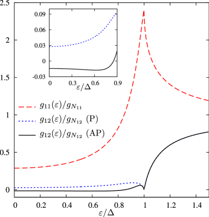
Figure 9: Local (long-dashed line) and non-local (short-dashed and solid lines) spectral conductances normalized to its normal state values. Here we choose $r_{N_{1}}=r_{N_{2}}=5r_{\xi_{S}}(0)$, $x_{1}=L-x_{2}=5\xi_{S}(0)$, $x_{2}-x_{1}=\xi_{S}(0)$, $G_{T_{1}}=G_{T_{2}}=4G_{m_{1}}=4G_{m_{2}}=0.2/r_{\xi_{S}}(0)$. Energy dependence of non-local conductance is displayed for parallel (P) $\bm{m}_{1}\bm{m}_{2}=1$ and antiparallel (AP) $\bm{m}_{1}\bm{m}_{2}=-1$ interface magnetizations. Inset: The same in the limit of low energies.

The second term in (135) is proportional to the product $\bm{m}_{1}\bm{m}_{2}G_{m1}G_{m2}$ and describes non-local magnetoconductance effect in our system emerging due to spin-sensitive electron scattering at FS interfaces. It is important that – despite the strong inequality $|G_{mi}|\ll G_{Ti}$ – both terms in Eq. (135) can be of the same order, i.e. the second (magnetic) contribution can significantly modify the non-local conductance of our device.

In the limit of large interface resistances $r_{N_{1,2}}g_{T1,2}(\varepsilon)\ll 1$ the formula (135) reduces to a much simpler one

$$g_{12}(\varepsilon)=g_{21}(\varepsilon)=\dfrac{r_{\xi_{S}}(\varepsilon)}{2}\exp[-d/\xi_{S}(\varepsilon)]\\ \times\left[\dfrac{\Delta^{2}-\varepsilon^{2}}{\Delta^{2}}g_{T1}(\varepsilon)g_{T2}(\varepsilon)+\bm{m}_{1}\bm{m}_{2}G_{m1}G_{m2}\dfrac{\Delta^{2}}{\Delta^{2}-\varepsilon^{2}}\right].$$ (138)

Interestingly, Eq. (138) remains applicable for arbitrary values of the angle between interface polarizations $\bm{m}_{1}$ and $\bm{m}_{2}$ and strongly resembles the analogous result for the non-local conductance in ballistic FSF systems (cf., e.g., Eq. (77) in the previous section). The first term in the square brackets in Eq. (138) describes the fourth order contribution in the interface transmissions which remains nonzero also in the limit of the nonferromagnetic leads GKZ . In contrast, the second term is proportional to the product of transmissions of both interfaces, i.e. only to the second order in barrier transmissions. This term vanishes identically provided at least one of the interfaces is spin-isotropic.

Contrary to the non-local conductance at subgap energies, both local conductance (at all energies) and non-local spectral conductance at energies above the superconducting gap are only weakly affected by magnetic effects. Neglecting small corrections due to $G_{m}$ term in the boundary conditions we obtain

$$\hat{g}_{11}(\varepsilon)=\hat{R}_{1}^{T}(\hat{\mathcal{M}}^{T})^{-1},\quad\hat{g}_{22}(\varepsilon)=\hat{R}_{2}^{T}(\hat{\mathcal{M}}^{T})^{-1},$$ (139)

$$\hat{g}_{12}(\varepsilon)=g_{21}(\varepsilon)=\hat{R}_{12}^{T}(\hat{\mathcal{M}}^{T})^{-1},\quad|\varepsilon|>\Delta.$$ (140)

Eqs. (139) and (140) together with the above expressions for the non-local subgap conductance enable one to recover both local and non-local spectral conductances of our system at all energies. Typical energy dependencies for both $g_{11}(\varepsilon)$ and $g_{12}(\varepsilon)$ are displayed in Fig. 9. For instance, we observe that at subgap energies the non-local conductance $g_{12}$ changes its sign being positive for parallel and negative for antiparallel interface polarizations.

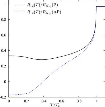
Figure 10: Non-local resistance (normalized to its normal state value) versus temperature (normalized to the superconducting critical temperature $T_{C}$) for parallel (P) and antiparallel (AP) interface magnetizations. The parameters are the same as in Fig. 9.

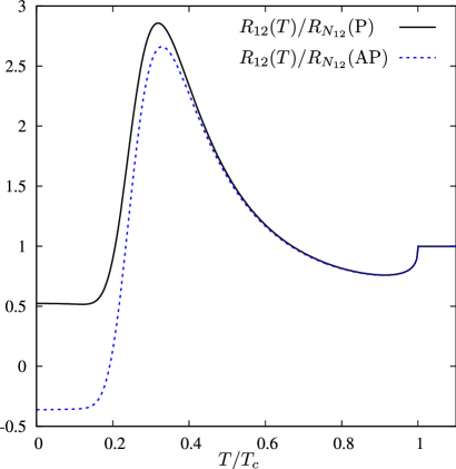
Figure 11: The same as in Fig. 10 for the following parameter values: $r_{N_{1}}=r_{N_{2}}=5r_{\xi_{S}}(0)$, $x_{1}=L-x_{2}=5\xi_{S}(0)$, $x_{2}-x_{1}=\xi_{S}(0)$, $G_{T_{1}}=G_{T_{2}}=25G_{m_{1}}=25G_{m_{2}}=0.025/r_{\xi_{S}}(0)$.

0.3.4 I-V curves

Having established the spectral conductance matrix $g_{ij}(\varepsilon)$ one can easily recover the complete $I-V$ curves for our hybrid FSF structure. In the limit of low bias voltages these $I-V$ characteristics become linear, i.e.

$$I_{1}=G_{11}(T)V_{1}-G_{12}(T)V_{2},$$ (141)

$$I_{2}=-G_{21}(T)V_{1}+G_{22}(T)V_{2},$$ (142)

where $G_{ij}(T)$ represent the linear conductance matrix defined as

$$G_{ij}(T)=\dfrac{1}{4T}\int g_{ij}(\varepsilon)\dfrac{d\varepsilon}{\cosh^{2}\dfrac{\varepsilon}{2T}}.$$ (143)

It may also be convenient to invert the relations (141)-(142) thus expressing induced voltages $V_{1,2}$ in terms of injected currents $I_{1,2}$:

$$V_{1}=R_{11}(T)I_{1}+R_{12}(T)I_{2},$$ (144)

$$V_{2}=R_{21}(T)I_{1}+R_{22}(T)I_{2},$$ (145)

where the coefficients $R_{ij}(T)$ define local ($i=j$) and nonlocal ($i\neq j$) resistances

$$R_{11}(T)=\dfrac{G_{22}(T)}{G_{11}(T)G_{22}(T)-G_{12}^{2}(T)},$$ (146)

$$R_{12}(T)=R_{21}(T)=\dfrac{G_{12}(T)}{G_{11}(T)G_{22}(T)-G_{12}^{2}(T)}$$ (147)

and similarly for $R_{22}(T)$. In non-ferromagnetic NSN structures the low temperature non-local resistance $R_{12}(T\to 0)$ turns out to be independent of both the interface conductances and the parameters of the normal leads GKZ . However, this universality of $R_{12}$ does not hold anymore provided non-magnetic normal metal leads are substituted by ferromagnets. Non-local linear resistance $R_{12}$ of our FSF structure is displayed in Figs. 10, 11 as a function of temperature for parallel ($\bm{m}_{1}\bm{m}_{2}=1$) and antiparallel ($\bm{m}_{1}\bm{m}_{2}=-1$) interface magnetizations. In Fig. 10 we show typical temperature behavior of the non-local resistance for sufficiently transparent interfaces. For both mutual interface magnetizations $R_{12}$ first decreases with temperature below $T_{C}$ similarly to the non-magnetic case. However, at lower $T$ important differences occur: While in the case of parallel magnetizations $R_{12}$ always remains positive and even shows a noticeable upturn at sufficiently low $T$, the non-local resistance for antiparallel magnetizations keeps monotonously decreasing with $T$ and may become negative in the low temperature limit. In the limit of very low interface transmissions the temperature dependence of the non-local resistance exhibits a well pronounced charge imbalance peak (see Fig. 11) which physics is similar to that analyzed in the case of non-ferromagnetic NSN structures GZ07 ; KZ08 ; GKZ . Let us point out that the above behavior of the non-local resistance is qualitatively consistent with available experimental observations Beckmann . More experiments would be desirable in order to quantitatively verify our theoretical predictions.

0.4 Concluding remarks

In this paper we developed a non-perturbative theory of non-local electron transport in both ballistic and diffusive NSN and FSF three-terminal structures with spin-active interfaces. Our theory is based on the quasiclassical formalism of energy-integrated Green-Eilenberger functions supplemented by appropriate boundary conditions describing spin-dependent scattering at NS and FS interfaces. Our approach applies at arbitrary interface transmissions and allows to fully describe non-trivial interplay between spin-sensitive normal scattering, local and non-local Andreev reflection at NS and FS interfaces.

In the case of ballistic structures our main results are the general expressions for the non-local cross-current $I_{12}$, Eq. (70), and for the non-local correction $I_{11}$ to the BTK current, Eq. (82). These expressions provide complete description of the conductance matrix of our three-terminal NSN device at arbitrary voltages, temperature, spin-dependent transmissions of NS interfaces and their polarizations. One of our important observations is that in the case of ballistic electrodes no crossed Andreev reflection can occur in both NSN and HSH structures with fully open interfaces. Beyond the tunneling limit the dependence of the non-local conductance on the size of the S-electrode $L$ is in general non-exponential and reduces to $G_{12}\propto\exp(-2L\Delta/v_{F})$ only in the limit of large $L$. For hybrid structures half-metal-superconductor-half-metal we predict that the low energy non-local conductance does not vanish already in the lowest order in barrier transmissions $G_{12}\propto D_{1\uparrow}D_{2\uparrow}$.

In the second part of our paper we addressed spin-resolved non-local electron transport in FSF structures in the presence of disorder in the electrodes. Within our model transfer of electrons across FS interfaces is described in the tunneling limit and magnetic properties of the system are accounted for by introducing ($i$) exchange fields $\bm{h}_{1,2}$ in both normal metal electrodes and ($ii$) magnetizations $\bm{m}_{1,2}$ of both FS interfaces. The two ingredients ($i$) and ($ii$) of our model are in general independent from each other and have different physical implications. While the role of (comparatively large) exchange fields $h_{1,2}\gg\Delta$ is merely to suppress disorder-induced interference of electrons VZK ; HN ; Z penetrating from a superconductor into ferromagnetic electrodes, spin-sensitive electron scattering at FS interfaces yields an extra contribution to the non-local conductance which essentially depends on relative orientations of the interface magnetizations. For anti-parallel magnetizations the total non-local conductance $g_{12}$ and resistance $R_{12}$ can turn negative at sufficiently low energies/temperatures. At higher temperatures the difference between the values of $R_{12}$ evaluated for parallel and anti-parallel magnetizations becomes less important. At such temperatures the non-local resistance behaves similarly to the non-magnetic case demonstrating, e.g., a well-pronounced charge imbalance peak GKZ in the limit of low interface transmissions.

Our predictions can be directly used for quantitative analysis of experiments on non-local electron transport in hybrid FSF structures.

Acknowledgments

This work was supported in part by DFG and by RFBR grant 09-02-00886. M.S.K. also acknowledges support from the Council for grants of the Russian President (Grant No. 89.2009.2) and from the Dynasty Foundation.

References

- (1) A.F. Andreev, Zh. Eksp. Teor. Fiz. 46, 1823 (1964) [Sov. Phys. JETP 19, 1228 (1964)].
- (2) G.E. Blonder, M. Tinkham, and T.M. Klapwijk, Phys. Rev. B 25, 4515 (1982).
- (3) J.M. Byers and M.E. Flatte, Phys. Rev. Lett. 74, 306 (1995).
- (4) G. Deutscher and D. Feinberg, Appl. Phys. Lett. 76, 487 (2000).
- (5) D. Beckmann, H.B. Weber, and H. v. Löhneysen, Phys. Rev. Lett. 93, 197003 (2004); D. Beckmann and H. v. Löhneysen, Appl. Phys. A 89, 603 (2007).
- (6) S. Russo, M. Kroug, T.M. Klapwijk, and A.F. Morpurgo, Phys. Rev. Lett. 95, 027002 (2005).
- (7) P. Cadden-Zimansky and V. Chandrasekhar, Phys. Rev. Lett. 97, 237003 (2006) .
- (8) P. Cadden-Zimansky, Z. Jiang, and V. Chandrasekhar, New J. Phys. 9, 116 (2007).
- (9) A. Kleine , A. Baumgartner, J. Trbovic and C. Schönenberger, Europhys. Lett. 87, 27011 (2009).
- (10) B. Almog, S. Hacohen-Gourgy, A. Tsukernik, and G. Deutscher, Phys. Rev. B 80, 220512(R) (2009).
- (11) A. Kleine, A. Baumgartner, J. Trbovic, D.S. Golubev, A.D. Zaikin, and C. Schönenberger, Nanotechnology 21, 274002 (2010).
- (12) J. Brauer, F. Hübler, M. Smetanin, D. Beckmann, and H. v. Löhneysen, Phys. Rev. B 81, 024515 (2010).
- (13) G. Falci, D. Feinberg, and F.W.J. Hekking, Europhys. Lett. 54, 255 (2001).
- (14) M.S. Kalenkov and A.D. Zaikin, Phys. Rev. B 75, 172503 (2007).
- (15) A. Brinkman and A.A. Golubov, Phys. Rev. B 74, 214512 (2006).
- (16) J.P. Morten, A. Brataas, and W. Belzig, Phys. Rev. B 74, 214510 (2006).
- (17) S. Duhot and R. Melin, Phys. Rev. B 75, 184531 (2007).
- (18) D.S. Golubev and A.D. Zaikin, Phys. Rev. B 76, 184510 (2007).
- (19) A. Levy Yeyati, F.S. Bergeret, A. Martin-Rodero, and T.M. Klapwijk, Nat. Phys. 3, 455 (2007).
- (20) M.S. Kalenkov and A.D. Zaikin, Phys. Rev. B 76, 224506 (2007).
- (21) M.S. Kalenkov and A.D. Zaikin, Physica E 40, 147 (2007).
- (22) M.S. Kalenkov and A.D. Zaikin, JETP Lett. 87, 140 (2008).
- (23) D.S. Golubev and A.D. Zaikin, Europhys. Lett. 86, 37009 (2009).
- (24) D.S. Golubev, M.S. Kalenkov, and A.D. Zaikin, Phys. Rev. Lett. 103, 067006 (2009).
- (25) F.S. Bergeret and A. Levy Yeyati, Phys. Rev. B 80, 174508 (2009).
- (26) D.S. Golubev and A.D. Zaikin, Phys. Rev. B 82, (2010).
- (27) A.F. Volkov, A.V. Zaitsev, and T.M. Klapwijk, Physica C 210, 21 (1993).
- (28) F.W.J. Hekking and Yu.V. Nazarov, Phys. Rev. Lett. 71, 1625 (1993).
- (29) A.D. Zaikin, Physica B 203, 255 (1994).
- (30) A. Huck, F.W.J. Hekking, and B. Kramer, Europhys. Lett. 41, 201 (1998).
- (31) A.V. Galaktionov and A.D. Zaikin, Phys. Rev. B 73, 184522 (2006).
- (32) W. Belzig, F.K. Wilhelm, C. Bruder, G. Schön, and A.D. Zaikin, Superlatt. Microstruct. 25, 1251 (1999).
- (33) M. Eschrig, Phys. Rev. B 61, 9061 (2000).
- (34) E. Zhao, T. Löfwander, and J.A. Sauls, Phys. Rev. B 70 134510 (2004).
- (35) A.V. Zaitsev, Sov. Phys. JETP 59, 1015 (1984).
- (36) A. Millis, D. Rainer, and J.A. Sauls, Phys. Rev. B 38 4504 (1988).
- (37) M. Eschrig, Phys. Rev. B 80, 134511 (2009).
- (38) A.V. Galaktionov and A.D. Zaikin, Phys. Rev. B 65, 184507 (2002).
- (39) M. Ozana and A. Shelankov, Phys. Rev. B 65, 014510 (2002).
- (40) E. Zhao and J.A. Sauls, Phys. Rev. Lett. 98, 206601 (2007).
- (41) M. Fogelström, Phys. Rev. B 62, 11 812 (2000).
- (42) Yu.S. Barash and I.V. Bobkova, Phys. Rev. B 65, 144502 (2002).
- (43) D. Huertas-Hernando, Yu.V. Nazarov, and W. Belzig, Phys. Rev. Lett. 88, 047003 (2002).
- (44) A. Cottet, D. Huertas-Hernando, W. Belzig, and Yu.V. Nazarov, Phys. Rev. B 80, 184511 (2009).