Algorithms to automatically quantify the geometric similarity of anatomical surfaces

Abstract

We describe new approaches for distances between pairs of 2-dimensional surfaces (embedded in 3-dimensional space) that use local structures and global information contained in inter-structure geometric relationships. We present algorithms to automatically determine these distances as well as geometric correspondences.
This is motivated by the aspiration of students of natural science to understand the continuity of form that unites the diversity of life. At present, scientists using physical traits to study evolutionary relationships among living and extinct animals analyze data extracted from carefully defined anatomical correspondence points (landmarks). Identifying and recording these landmarks is time consuming and can be done accurately only by trained morphologists. This renders these studies inaccessible to non-morphologists, and causes phenomics to lag behind genomics in elucidating evolutionary patterns.
Unlike other algorithms presented for morphological correspondences our approach does not require any preliminary marking of special features or landmarks by the user. It also differs from other seminal work in computational geometry in that our algorithms are polynomial in nature and thus faster, making pairwise comparisons feasible for significantly larger numbers of digitized surfaces. We illustrate our approach using three datasets representing teeth and different bones of primates and humans, and show that it leads to highly accurate results.

To document and understand physical and biological phenomena (e.g., geological sedimentation, chemical reactions, ontogenetic development, speciation, evolutionary adaptation, etc.), it is important to quantify the similarity or dissimilarity of objects affected or produced by the phenomena under study. The grain size or elasticity of rocks, geographic distances between populations, or hormone levels and body masses of individuals – these can be readily measured, and the resulting numerical values can be used to compute similarities/distances that help build understanding. Other properties like genetic makeup or gross anatomical structure can not be quantified by a single number; determining how to measure and compare these is more involved [34, 36, 50, 53]. Representing the structure of a gene (through sequencing) or quantification of an anatomical structure (through the digitization of its surface geometry) leads to more complex numerical representations; even though these are not measurements allowing direct comparison with their counterparts for other genes or anatomical structures, they represent an essential initial step for such quantitative comparisons. The 1-dimensional, sequential arrangement of genomes and the discrete variation (four nucleotide base types) for each of thousands of available correspondence points help reduce the computational complexity of determining the most likely alignment between genomes; alignment procedures are now increasingly automated [18]. The resulting, rapidly generated and massive data sets, analyzed with increasing sophistication and flexible in-depth exploration due to advances in computing technology, have lead to spectacular progress. For instance phylogenetics has begun to unravel mysteries of large scale evolutionary relationships experienced as extraordinarily difficult by morphologists [19].

Analyses of massive developmental and genetic data sets outpace those on morphological data. The comparative study of gross anatomical structures has lagged behind mainly because it is harder to determine corresponding parts on different samples, a prerequisite for measurement. The difficulty stems from the higher dimension (2 for surfaces vs. 1 for genomes), the continuous rather than discrete nature of anatomical objects, and from large shape variations.

In standard morphologists’ practice, correspondences are first assessed visually; then, some (10 to 100, at most) feature points can usually be defined as equivalent and/or identified as landmarks. Just as comparisons of tens of thousands of nucleotide base positions are used to determine similarity among genomes, the coordinates of these dozens of feature points (or measurements they define) are used to evaluate patterns of shape variation and similarity/difference [42]. However, as stated in 1936 by G. G. Simpson, the paleontologist chaperon of the Modern Synthesis in the study of evolution, the “difficulty in acquiring personal knowledge” ([21] p. 3) of morphological evidence limits our understanding of the evolutionary significance of morphological diversity; this remains true today. New techniques for generating and analyzing digital representations have led to major advances (see, e.g. [25, 22, 23]), but they typically still require determinations of anatomical landmarks by observers whose skill of identifying anatomical correspondences takes many years of training.

Several groups have sought to determine automatic correspondence among morphological structures. Existing successful methods typically introduce an effective dimensional reduction, using, e.g., 2-D outlines and/or images [54], or, in one of the few studies attempting automatic biological correspondences in 3-D as a method for evolutionary morphologists, “automatically-detected crest lines” [26] on surfaces obtained by CT-scans to register modern human skulls to each other [27] or to pre-Neanderthal, Homo heidelbergensis skulls [28]; another example is Wiley et al [25]. Studies using 2-D outlines or images sacrifice a lot of the original geometric information available in the 3-D objects on which they are based; such specifically limited representations cannot easily be incorporated into other studies. More generally and most importantly, none of these methods are independent of user input. When outlines or standard 2-D views are used, precise observations of the 3-D anatomical structures are required by the trained technician who creates the outlines or 2-D views [48, 47]. Several methods for 3-D alignment use Iterative Closest Point (ICP) algorithms [29] that require observer input to fix an initial guess (then further improved via local optimization); ICP-generated correspondences can also have large distortions and discontinuities of shape. In [7, 9] surfaces are matched by using the Gromov-Hausdorff distances between them, and applications to several shape analysis problems are given. However, Gromov-Hausdorff distances are hard to compute, and have to be approximated; the gradient descent optimization used in practice does not guarantee convergence to a global (rather than local) minimum.

Determination of correspondences or similarities among 3-D digitizations of general anatomic surfaces that is both 1) fully automated and 2) computationally fast (to handle the large data sets that are becoming increasingly available as imaging technologies become more widespread and efficient [40]) is still elusive. Our aim here is to remedy this by fully automating the determination of correspondences among gross anatomical structures. Success in this pursuit will help bring to phenomic studies the rate, objectivity and exhaustiveness of genomic studies. Large scale initiatives to phenotype model species after systematically knocking out each gene [38], as well as analysis of computational simulations of organogenesis [39] stand to greatly benefit from automating the determination of correspondence among, and measurement of, morphological structures.

In this paper, we describe several new distances between surfaces that can be used for such fully automated anatomic correspondences, and we test their relevance for biologically meaningful tasks on several anatomical dataset examples (high resolution digitizations of bones and teeth).

The paper is organized as follows. Section 1 gives the mathematical background for our algorithms: conformal geometry and optimal mass transportation (also known as Earth Mover’s distance). In section 2, we use these ingredients to define new distances or measures of dissimilarity, including a generalization to surfaces of the Procrustes distance. Section 3 presents the results obtained by our algorithms for three different morphological data sets, and an application.

No technical advance stands on its own; this paper is no exception. Conformal geometry is a powerful mathematical tool (permitting the reduction of the study of surfaces embedded in 3-D space to 2-D problems) that has been useful in many computational problems; [4] provides an introduction to both theory and algorithms, with many applications, including the use of conformal images of anatomical structures, combined with user prescribed landmarks and/or special features, for registration purposes, seeking “optimal” correspondence between pairs of surfaces [6]. Earth Mover’s distances [5] and continuous optimal mass transportation [1] have been used in image registration and for more general image analysis and parameterization [2]; in [8] (quadratic) mass transportation is used to relax the notion of Gromov-Hausdorff distance. Procrustes distances for discrete point sets are familiar to morphologists and other researchers working on shape analysis [23, 42]. The mathematical and algorithmic contribution of our work is the combination in which we use and generalize these ingredients to construct novel distance metrics, paired with efficient, fully automatic algorithms not requiring user guidance. They open the door to new applications requiring a large number of distance computations.

1 1. The mathematical components

1.1 Conformal geometry

 A mapping $\varphi$ from one 2-dimensional (smooth) surface $\mathcal{S}$ to another, $\mathcal{S}^{\prime}$, defines for every point $p\in\mathcal{S}$ a corresponding point $\varphi(p)\in\mathcal{S}^{\prime}$. If the mapping is smooth itself, it maps a smooth curve $\Gamma$ on $\mathcal{S}$ to a corresponding smooth curve $\Gamma^{\prime}$ on $\mathcal{S}^{\prime}$ that is called the image of $\Gamma$. Two curves $\Gamma_{1}$ and $\Gamma_{2}$ on $\mathcal{S}$ that intersect in a point $s$ are mapped to curves $\Gamma_{1}^{\prime}$, $\Gamma_{2}^{\prime}$ that intersect as well, in $s^{\prime}=\varphi(s)$. Consider the two (straight) lines $\ell_{1}$ and $\ell_{2}$ that are tangent to the curves $\Gamma_{1}$ and $\Gamma_{2}$ at their intersection point $s$; the angle between $\Gamma_{1}$ and $\Gamma_{2}$ at $s$ is then taken to mean the angle between the two lines $\ell_{1}$ and $\ell_{2}$; similarly, the angle between the curves $\Gamma_{1}^{\prime}$ and $\Gamma_{2}^{\prime}$ (at $s^{\prime}=\varphi(s)$) is the angle between their tangent lines at $s^{\prime}$. The mapping $\varphi$ is called conformal if for any two smooth curves $\Gamma_{1}$ and $\Gamma_{2}$ on $\mathcal{S}$, the angle between their images $\Gamma_{1}^{\prime}$ and $\Gamma_{2}^{\prime}$ is the same as that between $\Gamma_{1}$ and $\Gamma_{2}$ at the corresponding intersection point.

Riemann’s uniformization theorem [4] guarantees that every (reasonable) 2-d surface $\mathcal{S}$ in our standard 3-d space that is a disk-type surface (i.e. that has a boundary but no holes) can be mapped conformally to the 2-d unit disk $\mathbf{D}=\left\{z\ \mid\ z=x+\mbox{\rm\footnotesize{i}}y,\,\left|z\right|\leq 1\right\}$, with the boundary of the disk corresponding to the boundary of $\mathcal{S}$. This mapping is called “conformally flattening” . This flattening process is accompanied by area distortion; the conformal factor $f(x,y)$ on the disk, varying from point to point, indicates the area distortion factor produced by the operation.

One important practical implication of this theorem is that the family of conformal maps between two surfaces can be characterized naturally via the flattened representations of the surfaces: if $\gamma$ is a conformal mapping from $\mathcal{S}$ to $\mathcal{S}^{\prime}$, and $\varphi$ ($\varphi^{\prime}$) is a flattening (i.e. a conformal map to the disk $\mathbf{D}$) of $\mathcal{S}$ ($\mathcal{S}^{\prime}$), then the family of all possible conformal mappings from $\mathcal{S}$ to $\mathcal{S}^{\prime}$ is given by $\gamma={\varphi^{\prime}}^{-1}\circ m\circ\varphi$, where $m$ ranges over all the conformal bijective self-mappings of the unit disk $\mathbf{D}$. We shall call such $m$ disk-preserving Möbius transformations; they constitute a group, the disk-preserving Möbius transformation group $\mathcal{M}$. Each $m$ in $\mathcal{M}$ is characterized by 3 parameters and given by the closed-form formula $m(z)=e^{\mbox{\rm\footnotesize{i}}\theta}(z-\alpha)(1-z\bar{\alpha})^{-1}$, where $\theta\in[0,2\pi)$, $|\alpha|<1$. For our applications, it is important that the flattening process (starting from a triangulated digitized version of $\mathcal{S}$) and more importantly the disk-preserving Möbius transformations can be computed fast and with high accuracy; for more details, see [16, 15]. Note that the flattening map of a surface $\mathcal{S}$ is not unique; one can choose any arbitrary point of $\mathcal{S}$ to be mapped to the origin of the disk $\mathbf{D}$, and any direction through this point to become the “$x$-axis”. The transition from choosing one (center, direction) pair to another is simply a disk-preserving Möbius transformation. It is convenient to equip the disk $\mathbf{D}$ with its hyperbolic measure $d\eta(x,y)\,=\,[1-(x^{2}+y^{2})]^{-2}dx\,dy$, invariant with respect to Möbius transformations; correspondingly, we set $\mathbf{f}(x,y)=[1-(x^{2}+y^{2})]^{2}\,f(x,y)$, so that $\mathbf{f}\,d\eta\,=\,f\,dx\,dy\,$.

1.2 Optimal mass transportation

 An integrable function $\mu$ is a (normalized) mass distribution on a domain $D$ if $\mu(u)\geq 0$ is well defined for each $u\in D$, and $\int_{D}\mu(u)\,du\,=\,1$. If $\tau$ is a differentiable bijection from $D$ to itself, the mass distribution $\mu^{\prime}=\tau_{*}\mu$ on $D$ defined by $\mu(u)=\mu^{\prime}(\tau(u))\,J_{\tau}(u)$ (where $J_{\tau}$ is the Jacobian of the map $\tau$), is the transportation (or push-forward) of $\mu$ by $\tau$ in the sense that, for any arbitrary (non pathological) function $F$ on $D$, $\int_{D}F(u)\,\mu^{\prime}(u)\,du\,=\,\int_{D}F(\tau(u))\,\mu(u)\,du$. The total transportation effort is given by $\mathcal{E}_{\tau}\,=\,\int_{D}d(u,\tau(u))\,\mu(u)\,du$, where $d(u,v)$ denotes the distance between two points $u$ and $v$ in $D$.
If two mass distributions $\mu$ and $\nu$ on $D$ are given, then the optimal mass transportation distance between $\mu$ and $\nu$ (in the sense of Monge, see [10], p. 4) is the infimum of the transportation effort $\mathcal{E}_{\tau}$, taken over all the measurable bijections $\tau$ from $D$ to $D$ for which $\nu$ equals the transportation of $\mu$ by $\tau$. This set of bijections is hard to search; the determination of an optimal mass transportation scheme becomes more tractable if the mass “at $u$” need not all end up at the same end point. One then considers measures $\pi$ on $D\times D$ with marginals $\mu$ and $\nu$ (this means that for all continuous functions $F,G$ on $D$, $\int_{D\times D}F(u)\,d\pi(u,v)$ $=$ $\int_{D}F(u)\,\mu(u)\,du$ and $\int_{D\times D}G(v)\,d\pi(u,v)$ $=$ $\int_{D}G(v)\,\nu(v)\,dv$); the optimal mass transportation in this more general Kantorovitch formulation is the infimum over all such measures $\pi$ of $E_{\pi}$ $=$ $\int_{D\times D}d(u,v)\,d\pi(u,v)$. A comprehensive treatment of optimal mass transport is in [10].

2 2. New distances between 2-dimensional surfaces

2.1 Conformal Wasserstein distance (cW)

  One can use optimal mass transport to compare conformal factors $\mathbf{f}$ and $\mathbf{f}^{\prime}$ obtained by conformally flattening two surfaces, $\mathcal{S}$ and $\mathcal{S}^{\prime}$. If $m$ is a disk-preserving Möbius transformation, then $\mathbf{f}$ and $m_{*}\mathbf{f}=\mathbf{f}\circ m^{-1}$ are both equally valid conformal factors for $\mathcal{S}$. A standard approach to take this into account is to “quotient” over $\mathcal{M}$, which leads to the conformal Wasserstein distance:

$$\mbox{\hausaD}_{\mbox{\small{cW}}}(\mathcal{S},\mathcal{S}^{\prime})\!=\!\!\inf_{m\in\mathcal{M}}\!\left[\inf_{\pi\in\Pi(m_{*}\mathbf{f},{\mathbf{f}}^{{}^{\prime}})}\!\int_{\mathbf{D}\times\mathbf{D}}\!\!\!\!\!\!\widetilde{d}\big{(}z,z^{\prime}\big{)}d\pi(z,z^{\prime})\right],$$ (1)

where $\widetilde{d}(\cdot,\cdot)$ is the (conformally invariant) hyperbolic distance in $\mathbf{D}$; $\mbox{\hausaD}_{\mbox{\small{cW}}}$ satisfies then all the properties of a metric [12]. In particular, $\mbox{\hausaD}_{\mbox{\small{cW}}}(\mathcal{S},\mathcal{S}^{\prime})=0$ iff $\mathcal{S}$ and $\mathcal{S}^{\prime}$ are isometric. However, computing this metric requires solving a Kantorovitch mass-transportation problem for every candidate $m$; even though the whole procedure has polynomial runtime complexity, it is too heavy to be used in practice for large datasets.

2.2 Conformal Wasserstein neighborhood dissimilarity distance (cWn)

  We propose another natural way to use Kantorovich’s optimal mass transport to compare surfaces $\mathcal{S}$ and $\mathcal{S}^{\prime}$. Instead of determining the most efficient way to transport “mass” $\mathbf{f}$ from $z$ to $z^{\prime}$, we can quantify how dissimilar the “landscapes” are, defined by $\mathbf{f}$ and $\mathbf{f}^{\prime}$ near $z$, resp. $z^{\prime}$, and replace the distance $\widetilde{d}(\cdot,\cdot)$ by a measure of neighborhood dissimilarity. The neighborhood $N(0,R)$ around $0$ is given by $N(0,R)=\{\,z\,;\,|z|<R\,\}$; neighborhoods around other points are obtained by letting the disk-preserving Möbius transformations act on $N(0,R)$: for any $m$ in $\mathcal{M}$ such that $z=m(0)$, $N(z,R)$ is the image of $N(0,R)$ under the mapping $m$. Next we define the dissimilarity between $\mathbf{f}$ at $z$ and $\mathbf{f}^{\prime}$ at $z^{\prime}$:

$$\mathbf{d}^{R}_{\mathbf{f},{\mathbf{f}}^{{}^{\prime}}}(z,z^{\prime})=\!\!\inf_{m\in\mathcal{M},m(z)=z^{\prime}}\!\left[\,\int_{N(z,R)}|\mathbf{f}(w)-\mathbf{f}^{\prime}(m(w))\,|\,d\eta(w)\right].$$

It is straightforward to check that for all $m,m^{\prime}$ in $\mathcal{M}$, $\mathbf{d}^{R}_{m_{*}\mathbf{f},{{m}^{{}^{\prime}}}_{*}{\mathbf{f}}^{{}^{\prime}}}(m(z),m^{\prime}(z^{\prime}))=\mathbf{d}^{R}_{\mathbf{f},{\mathbf{f}}^{{}^{\prime}}}(z,z^{\prime})$. We now use optimal transport, and define the conformal Wasserstein neighborhood dissimilarity distance between $\mathbf{f}$ and $\mathbf{f}^{\prime}$:

$$\mathcal{D}^{R}_{\mbox{\small{cWn}}}(\mathcal{S},\mathcal{S}^{\prime})\,=\,\inf_{\pi\in\Pi(\mathbf{f},{\mathbf{f}}^{{}^{\prime}})}\int_{\mathbf{D}{\color[rgb]{0.6,0,0}\times}\mathbf{D}}\mathbf{d}_{\mathbf{f},{\mathbf{f}}^{{}^{\prime}}}(z,z^{\prime})\,d\pi(z,z^{\prime})~{},$$ (2)

where the superscript recalls that this definition depends on the choice of the parameter $R$. For a proof that this defines a true distance between (generic) surfaces $\mathcal{S}$ and $\mathcal{S}^{\prime}$, and further mathematical properties, see [12, 13]. One practical difference with $\mbox{\hausaD}_{\mbox{\small{cW}}}$ is that (2) requires solving only one Kantorovitch mass-transportation problem once the special dissimilarity cost is computed, resulting in a simpler optimization problem. To implement the computation of these distances, we discretize the integrals and the optimization searches, picking collections of discrete points on the surfaces; the minimizing measure $\pi$ in the definition of $\mathcal{D}^{R}_{\mbox{\small{cWn}}}(\mathcal{S},\mathcal{S}^{\prime})$ can then be used to define a correspondence between points of $\mathcal{S}$ and $\mathcal{S}^{\prime}$.

2.3 Continuous Procrustes distance between surfaces (cP)

  Both cW and cWn are intrinsic: they use only information “visible” from within each surface, such as geodesic distances between pairs of points; consequently they do not distinguish a surface from any of its isometric embeddings in 3-D. The continuous Procrustes (cP) distance [14] described in this section uses some extrinsic information as well; it fails to distinguish two surfaces only if one is obtained by applying to the other a rigid motion (which is a very special isometry).

The (standard) Procrustes distance is defined between discrete sets of points $\mathbf{X}=(X_{n})_{n=1,\ldots,N}\subset\mathcal{S}$ and $\mathbf{Y}=(Y_{n})_{n=1,\ldots,N}\subset\mathcal{S}^{\prime}$ by minimizing over all rigid motions: $d_{P}(\mathbf{X},\mathbf{Y})\,=\,\min_{R\mbox{\small{ rig.mot.}}\!}\left[\,\left(\,\sum_{n=1}^{N}|R(X_{n})-Y_{n}|^{2}\,\right)^{1/2}\,\right]$, where $\left|\cdot\right|$ denotes the standard Euclidean norm. Often $\mathbf{X},\,\mathbf{Y}$ are sets of landmarks on two surfaces, and $d_{P}(\mathbf{X},\mathbf{Y})$ is interpreted as a distance between these surfaces. This practice has several drawbacks: 1) $d_{P}(\mathbf{X},\mathbf{Y})$ depends on the (subjective) choice of $\mathbf{X},\mathbf{Y}$, which makes it a not necessarily “well-defined” or easily reproducible proxy for a surface distance; 2) the (relatively) small number of $N$ landmarks on each surface disregards a wealth of geometric data; 3) identifying and recording the $x_{n},\,y_{n}$ is time consuming and requires expertise.

We eliminate all these drawbacks by a landmark-free approach, introducing the continuous Procrustes distance. Instead of relying on experts to identify “corresponding” discrete subsets of $\mathcal{S}$ and $\mathcal{S}^{\prime}$, we consider a family of continuous maps $a:\mathcal{S}\rightarrow\mathcal{S}^{\prime}$ between the surfaces, and rely on optimization to identify the “best” $a$. The earlier exact correspondence of one point $Y_{n}$ to one point $X_{n}$, and the (tacit) assumption that $\mathbf{X}$ ($\mathbf{Y}$) collectively represent all the noteworthy aspects of $\mathcal{S}$ ($\mathcal{S}^{\prime}$) in a balanced way, are recast as requiring that the “correspondence map” be area-preserving [14], that is, for every (measurable) subset $\Omega$ of $\mathcal{S}$, $\int_{\Omega}dA_{\mathcal{S}}=\int_{a(\Omega)}dA_{\mathcal{S}^{\prime}}$, where $dA_{\mathcal{S}}$ and $dA_{\mathcal{S}^{\prime}}$ are the area elements on the surfaces induced by their embeddings in $\mathbb{R}^{3}$. We denote $\mathcal{A}(\mathcal{S},\mathcal{S}^{\prime})$ the set of all these area-preserving diffeomorphisms. For each $a$ in $\mathcal{A}(\mathcal{S},\mathcal{S}^{\prime})$, we set $\mathbf{d}(\mathcal{S},\mathcal{S}^{\prime},a)^{2}=\min_{R\mbox{\small{ rig.mot.}}\!}\int_{\mathcal{S}}|R(x)-a(x)|^{2}dA_{\mathcal{S}}$; the continuous Procrustes distance between $\mathcal{S}$ and $\mathcal{S}^{\prime}$ is then

$$\mathbf{D}_{P}(\mathcal{S},\mathcal{S}^{\prime})=\inf_{a\in\mathcal{A}(\mathcal{S},\mathcal{S}^{\prime})}\mathbf{d}(\mathcal{S},\mathcal{S}^{\prime},a)~{}.$$ (3)

This defines a metric distance on the space of surfaces (up to rigid motions: for congruent surfaces the distance is 0) [14]. Minimizing over rigid motions is easy; there exist closed form formulas, as in the discrete case. But the second set over which to minimize, $\mathcal{A}(\mathcal{S},\mathcal{S}^{\prime})$, is an unwieldy, formally infinite-dimensional manifold, hard to explore. This is an optimal transport problem again, now in the much harder Monge formulation. For “reasonable” surfaces (e.g., surfaces with uniformly bounded curvature), transformations $a$ close to optimal are close to conformal [14]. This crucial insight allows limiting the search to the much smaller space of maps obtained by small deformations of conformal maps. Concretely, we compose a conformal map (represented as a Möbius transformation) $m\in\mathcal{M}$ with maps $\chi$ and $\varrho$, where $\varrho$ is a smooth map that roughly aligns high density peaks, and $\chi$ is a special deformation (following [41]) using local diffusion to make $\chi\circ\varrho\circ m$ area preserving (up to approximation error). For each choice of peaks $p,\,p^{\prime}$ in the conformal factors of $\mathcal{S}$, $\mathcal{S}^{\prime}$, the algorithm 1) runs through the 1-parameter family of $m$ that map $p$ to $p^{\prime}$; 2) constructs a map $\varrho$ that aligns the other peaks, as best possible; and 3) computes $\mathbf{d}(\mathcal{S},\mathcal{S}^{\prime},\varrho\circ m)$. Repeat for all choices of $p,\,p^{\prime}$; the $\varrho\circ m$ that minimizes $\mathbf{d}$ is then deformed to be area preserving, producing the map $a=\chi\circ\varrho\circ m$; $\mathbf{d}(\mathcal{S},\mathcal{S}^{\prime},a)$ and $a$ are our approximate $\mathbf{D}_{P}(\mathcal{S},\mathcal{S}^{\prime})$ and correspondence map, respectively. (More in Supplementary Materials.)

3 3. Application to anatomical datasets

To test our approach, we used three independent datasets, representing three different regions of the skeletal anatomy, of humans, other primates, and their close relatives. Digitized surfaces were obtained from High Resolution X-ray Computed Tomography ($\mu$CT) scans (see Supplementary Materials) of  (A) 116 second mandibular molars of prosimian primates and non-primate close relatives, and  (B) 57 proximal first metatarsals of prosimian primates, New and Old World monkeys, and  (C) 45 distal radii of apes and humans. For every pair of surfaces, the output of our algorithms consists of 1) a correspondence map for the whole surface (i.e. not just a few points), and 2) a non-negative number giving their dissimilarity (where zero means they are isometric or congruent). Typical running times for a pair of surfaces were $\sim 20$ sec. for cP, $\sim 5$ min. for cWn. To evaluate the performance of the algorithms, we compared the outcomes to those determined independently by morphologists. Using the same set of digitized surfaces, geometric morphometricians collected landmarks on each, in the conventional fashion [42], choosing them to reflect correspondences considered biologically and evolutionarily meaningful (see Supplementary Materials). These landmarks determine “discrete” Procrustes distances for every two surfaces (see $\mathsection$ 2), here called Observer-Determined Landmarks Procrustes (ODLP) distances. For each of the three distances we obtain thus a (symmetric) matrix.

3.1 Comparing the distance (dissimilarity) matrices

  We compare cWn- and cP- with ODLP-matrices in two different ways. Sets of distances are far from independent, and it is traditional to assess the relationship between distance matrices by a Mantel correlation analysis [43]: first correlate the entries in the two square arrays, and then compute the fraction, among all possible relabelings of the rows/columns for one of them, that leads to a larger correlation coefficient; this Mantel significance is a stronger indicator than the correlation coefficient itself. Table 1 gives the results for our datasets.

 

 

In all cases the Mantel significance between ODLP and cP distances is higher than that between ODLP and cWn. This

indicates that distances computed using cP match those determined by morphometricans’ better than those using cWn.

Figure 1 illustrates the relationship of cP, cWn, and ODLP distances in a different way. In each of the two square matrices (corresponding to cP and cWn, each vs. ODLP), the color of each pixel indicates the value of the entry (using a red-blue colormap, with deep blue representing 0, and saturated red the largest value); upper right triangular halves correspond to cP or cWn; (identical) lower left halves to ODLP. The same ordering of samples is used in the three cases, with samples ordered so that nearby samples typically have smaller distances. This type of display is especially good to compare the structure of two distance matrices for small distances, often the most reliable . Note the better symmetry along the diagonal for ODLP/cP comparison on the left: in this comparison, as in the previous one, cP outperforms cWn.

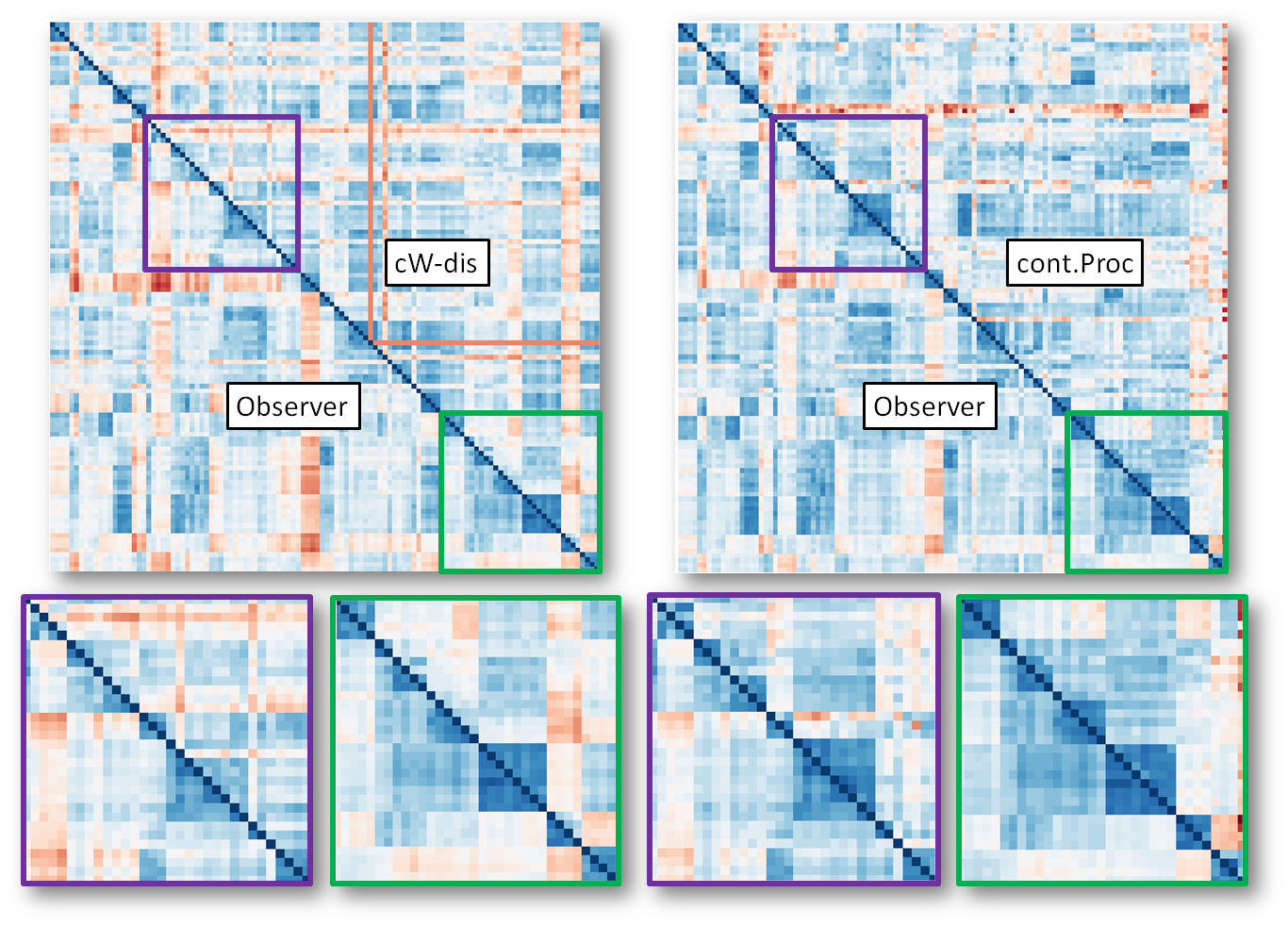
Figure 1: For small distances, the structures of the matrices with cP-, cWn-distances and distances based on Observer Landmarks (ODLP) are very similar, with cP (on the right) the most similar to ODLP. The dataset illustrated here is dataset (A).

3.2 Comparing scores in taxonomic classification

 Accurately placed ODL usually result in smaller ODLP distances between specimens representing individuals of the same species/genus than between individuals of different species/genera.

 

 

To assess whether this holds as well for the algorithmic cP and cWn distances, we run three taxonomic classification analyses on each data set, one using ODLP distances, and two using cP and cWn distances, with a “leave one out” procedure: each specimen (treated as unknown) is assigned to the taxonomic group of its nearest neighbor among the remainder of the specimens in the data set (treated as known). Table 2 lists success rates (in %) for three different classification queries for the three datasets. For each dataset $N$ is the number of objects; for each query $\#$ is the number of groups. Classifications based on the cP distances are similar in accuracy to those based on the ODLP distances, outperforming the cWn distances for all three of our anatomic datasets.

Note: a similar classification based on topographic variables is less accurate: for the 99 teeth belonging to 24 genera, only 54 (54 %) were classified correctly with a classification based on the four topographic variables Energy, Shearing Quotient, Relief Index, OPC. (Details in Supplementary Materials.)

3.3 Comparing the correspondence maps

  Morphometric analyses are based on the identification of corresponding landmark points on each of $\mathcal{S}$ and $\mathcal{S}^{\prime}$; the cP algorithm constructs a correspondence map $a$ from $\mathcal{S}$ to $\mathcal{S}^{\prime}$. (The correspondence induced by cWn is less smooth and will not be considered here.) For each landmark point $L$ on $\mathcal{S}$, we can compare the location on $\mathcal{S}^{\prime}$ of its images $a(L)$ with the location of the corresponding landmark points $L^{\prime}$. Fig. 2 shows that the “propagated” landmarks $a(L)$ typically turn out to be very close to those of the “true” landmarks $L^{\prime}$. (More in Supplementary Materials.)

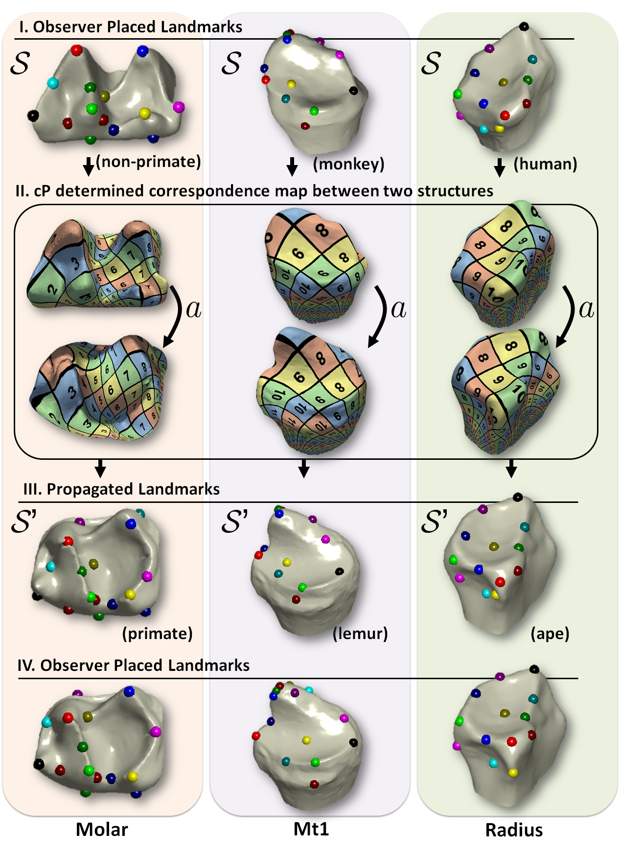
Figure 2: Observer-placed landmarks can be propagated from structure M (A) using cP determined correspondence maps (B) to another specimen N (C). The similarity between propagated landmarks in (C) and observer placed landmarks in (D) on N shows the success of the method, and makes explicit the geometric basis for the observer-determinations.

3.4 An application

These comparisons show our algorithms capture biologically informative shape variation. But scientists are interested in more than overall shape! We illustrate how correspondence maps could be used to analyze more specific features. In comparative morphological and phylogenetic studies, anatomical identification of certain features (e.g., particular cusps on teeth) is controversial in some cases; an example of this is the distolingual corner of sportive lemur ( Lepilemur) lower molars in our data set (A) [37, 36].

In such controversial cases, transformational homology [17] hypotheses are usually supported by a specific comparative sample or inferred morphocline [35, 52, 36]. Lepilemur is thought by some researchers to lack a cusp known as an entoconid (Fig. 3) but to have a hypertrophied metastylid cusp that “takes the place” of the entoconid [36] in other taxa. Yet, in comparing a Lepilemur tooth to a more “standard” primate tooth, like that of Microcebus, both seem to have the same basic cusps; alternatives to the viewpoint of [36] have therefore also been argued in the literature [37]. However, another lemur, Megaladapis (now extinct), arguably a closer relative of Lepilemur than Microcebus, has an entoconid that is very small and a metastylid that is rather large, thus providing an evolutionary argument supporting the original hypothesis. (For more details, see Supplementary Materials.) Such arguments can now be made more precise. We can propagate (as in Fig. 2) landmarks from the Microcebus to the Lepilemur molar; this direct propagation matches the entoconid cusp of Microcebus with the controversial cusp of Lepilemur (Fig. 3, path 1), supporting [37]. In contrast, when we propagate landmarks in different steps, either from Microcebus to Megaladapis and then to Lepilemur(Fig. 3, path 2), or through the extinct Adapis and extant Lemur (Fig. 3, path 3), the Lepilemur metastylid takes the place of the Microcebus entoconid, supporting [36]. Automatic propagation of landmarks via mathematical algorithms recenters the controversy on the (different) discussion of which propagation channel is most suitable.

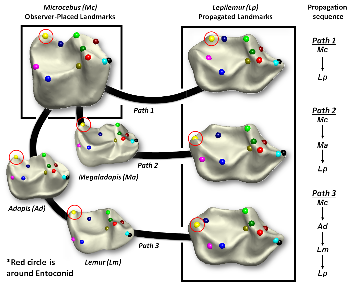
Figure 3: Observer-placed landmarks on a tooth of Microcebus are propagated using cP-determined correspondence maps to a tooth of Lepilemur. Path 1 is direct, Path 2 and 3 have intermediate steps, representing step-wise propagation between teeth of other taxa.

3.5 Summary and Conclusion

 New distances between 2-D surfaces, with fast numerical implementations, were shown to lead to fast, landmark-free algorithms that map anatomical surfaces automatically to other instances of anatomically equivalent surfaces, in a way that mimics accurately the detailed feature-point correspondences recognized qualitatively by scientists, and that preserves information on taxonomic structure as well as observer-determined-landmark distances. Moreover, the correspondence maps thus generated can incorporate, in their tracking of point features, evolutionary relationships inferred to link different taxa together.

Our approach makes morphology accessible to non-specialists and allows the documentation of anatomical variation and quantitative traits with previously unmatched comprehensiveness and objectivity. More frequent, rapid, objective, and comprehensive construction of morphological datasets will allow the study of morphological diversity’s evolutionary significance to be better synchronized with studies incorporating genetic and developmental information, leading to a better understanding of anatomical form and its genetic basis, as well as the evolutionary processes that have contributed to their diversity among living things on earth.

References

- [1] Haker S, Zhu L, Tannenbaum A, & Angenent S (2004) Optimal Mass Transport for Registration and Warping. Int. J. Comp. Vis. 60(3):225-240.
- [2] Dominitz A, & Tannenbaum A (201) Texture Mapping via Optimal Mass Transport. IEEE Transactions on Visualization and Computer Graphics, 16:419-433.
- [3] Zeng W, et al. (2008) 3D Non-rigid Surface Matching and Registration Based on Holomorphic Differentials. 10th Euro. Conf. Comp. Vis. (ECCV)
- [4] Gu X & Yau ST (2008) Computational Conformal Geometry. (International Press of Boston)
- [5] Rubner Y, Tomasi C, & Guibas LJ (2008) The Earth Mover’s Distance as a Metric For Image Retrieval. Int. J. Comp. Vis. 40(2):99-121.
- [6] Gu X, Wang Y, Chan TF, Thompson PM, & Yau ST (2004) Genus Zero Surface Conformal Mapping and Its Application to Brain Surface Mapping. Med. Img. 23(8):949-958; WWang Y, Lui L, Chan TF, & Thompson P (2005) Optimization of brain conformal mapping with landmarks. in MICCAI 8th Int. Conf. Med. Img. Computing and Computer Assisted Intervention (MICCAI); Lui L, Wang Y, Chan TF, & Thompson P (2007) Landmark constrained genus zero surface conformal mapping and its application to brain mapping research. Appl. Num. Math. 57:847-858.
- [7] Mémoli F & Guillermo Sapiro (2005) A Theoretical and Computational Framework for Isometry Invariant Recognition of Point Cloud Data. Found. Comput. Math. 5(3):313-347.
- [8] Mémoli F (2007) On the use of Gromov-Hausdorff Distances for Shape Comparison. SPBG07-proc.
- [9] A. M. Bronstein, M. M. Bronstein, & R. Kimmel (2006) Generalized multidimensional scaling: a framework for isometry-invariant partial surface matching. Proc. National Academy of Sciences (PNAS), 103(5):1168-1172.
- [10] Villani C (2003) Topics in Optimal Transportation. Grad. Stud. Math. ser., Amer. Math. Soc. 58. ; Villani C (2008) Optimal Transport: Old and New (Springer).
- [11] Mémoli F: Gromov-Hausdorff distances in Euclidean spaces, NORDIA-CVPR-2008.
- [12] Lipman Y & Daubechies I Conformal Wasserstein Distances: Comparing Surfaces in Polynomial Time. Advances in Mathematics (accepted for publication).
- [13] Lipman I & Daubechies Y (2010) Surface Comparison With Mass Transportation. At www.arxiv.org, arXiv:0912.3488v2 [math.NA].
- [14] Lipman Y, Al-Aifari R, Funkhouser T, & Daubechies I (in prep.) The Surface Procrustes Distance.
- [15] Lipman Y, Puente J, & Daubechies I (submitted) Conformal Wasserstein Distances: Comparing Disk and Sphere-type Surfaces in Polynomial Time II: Computational Aspects.
- [16] Lipman Y & Funkhouser T (2009) Mobius Voting for Surface Correspondence. ACM Trans. Graph. (Proc. SIGGRAPH 2009).
- [17] Patterson C (1982) Morphological characters and homology. Systematics Association Special Volume No. 21, ”Problems of Phylogenetic Reconstruction”, eds Joysey KA & Friday AE (Academic Press, London and New York), pp 21-74.
- [18] Liu K, Raghavan S, Nelesen S, Linder CR, & Warnow T (2009) Rapid and Accurate Large-Scale Coestimation of Sequence Alignments and Phylogenetic Trees. Science 324:1561-1564.
- [19] Murphy WJ, et al. (2001) Resolution of the early placental mammal radiation using Bayesian phylogenetics. Science 294(5550):2348-2351;
- [20] Owen R (1846) Report on the archetype and homologies of the vertebrate skeleton. Report of the British Association for the Advancement of Science (Southampton meeting):169-340.
- [21] Simpson GG (1936) Studies of the earliest mammalian dentitions. Dental Cosmos 78:791-800 and 940-953.
- [22] Polly PD & MacLeod N (2008) Locomotion in fossil Carnivora: An application of eigensurface analysis for morphometric comparison of 3D surfaces. Palaeontologia Electronica 11(2).
- [23] Zelditch ML, Swiderski DL, Sheets DH, & Fink WL (2004) Geometric Morphometrics for Biologists (Elsevier Academic Press, San Diego) p 425.
- [24] Ghosh D, Sharf A, & Amenta N (2009) Feature-driven deformation for dense correspondence. Proceedings of SPIE Medical Imaging 7261:36-40.
- [25] David F. Wiley, Nina Amenta, Dan A. Alcantara, Deboshmita Ghosh, Yong J. Kil, Eric Delson, Will Harcourt-Smith, F. James Rohlf, Katherine St. John, & Bernd Hamann (2005) Evolutionary Morphing. Proceedings of IEEE Visualization 2005:8.
- [26] Thirion JP & Gourdon A (1996) The 3D Marching Lines Algorithm. Graphical Models and Image Processing 58(6):503-509.
- [27] Subsol G, Thirion JP, & Ayache N (1998) A General Scheme for Automatically Building 3D Morphometric Anatomical Atlases : application to a Skull Atlas. Medical Image Analysis 2(1):37-60.
- [28] Subsol G, Mafart B, Silvestre A, & de Lumley MA (2002) 3d image processing for the study of the evolution of the shape of the human skull: presentation of the tools and preliminary results. Three-Dimensional Imaging in Paleoanthropology and Prehistoric Archaeology, BAR International Series, eds Mafart B, Delingette H, & Subsol G), pp 37-45.
- [29] Besl PJ & McKay ND (1992) A Method for Registration of 3-D Shapes. IEEE Trans. Pattern Anal. Mach. Intell. 14(2):239-256.
- [30] Lipman Y & Daubechies I (2010) Surface Comparison With Mass Transportation. Technical report, Princeton University.
- [31] Lipman Y & Funkhouser T (2009) Mobius Voting for Surface Correspondence. ACM Trans. Graphics (Proc. ACM SIGGRAPH) 28(3).
- [32] Gu X & Yau S-T (2003) Global conformal surface parameterization. SGP ’03: Proc. 2003 Eurographics/ACM SIGGRAPH symp. Geometry processing, (Eurographics Association, Aachen), pp 127-137.
- [33] Szalay FS & Dagosto M (1988) Evolution of Hallucial Grasping in the Primates. J. Hum. Evol. 17(1-2):1-33.
- [34] Sargis EJ, Boyer DM, Bloch JI, & Silcox MT (2007) Evolution of pedal grasping in Primates. J. Hum. Evol. 53:103-107.
- [35] Osborn HF (1907) Evolution of Mammalian Molar Teeth: To and From the Tritubercular Type (The Macmillan Company, New York) p 250;
- [36] Schwartz JH & Tattersall I (1985) Evolutionary Relationships of living lemurs and lorises (Mammalia, Primates) and their potential affinities with European Eocene Adapidae (Am. Mus. Nat. Hist., New York) p 100.
- [37] Swindler (2002) Primate Dentition: An Introduction to the Teeth of Non-Human Primates (Cambridge University Press, Cambridge) p 312.
- [38] Abbott A (2010) Mouse project to find each gene’s role. Nature 465:410.
- [39] Salazar-Ciudad I & Jernvall J (2010) A computational model of teeth and the developmental origins of morphological variation. Nature 464:583-586.
- [40] Schmidt EJ, et al. (2010) Micro-computed tomography-based phenotypic approaches in embryology: procedural artifacts on assessments of embryonic craniofacial growth and development. BMC Develop. Bio. 10(18).
- [41] Moser J (1965) On the Volume Elements on a Manifold, Trans. Am. Math. Soc. 120(2):286-294.
- [42] Mitteroecker P & Gunz P (2009) Advances in Geometric Morphometrics. Evol. Bio. 36:235-247.
- [43] Mantel N (1967) The detection of disease clustering and a generalized regression approach. Canc. Res. 27:209-220.
- [44] Kristensen E, Parsons TE, HallgrImsson B, & Boyd SK (2008) A Novel 3-D Image-Based Morphological Method for Phenotypic Analysis. IEEE Trans. Biomed. Eng. 55(12):2826-2831.
- [45] Shen L, Farid H, & McPeek MA (2009) Modeling three-dimensional morphological structures using spherical harmonics. Evolution 63(4):1003-1016.
- [46] Weeks PJD, Gauld ID, Gaston KJ, & O’Neill MA (1997) Automating the identification of insects: a new solution to an old problem. Bull. Entomol. Res. 87:203-211.
- [47] Weeks PJD, O’Neill MA, Gaston KJ, & Gauld ID (1999) Species-identification of wasps using principal component associative memories. Img. Vis. Comp. 17:861-866.
- [48] Gaston KJ & O’Neill MA (2004) Automated species identification-why not? Phil. Trans. R. Soc. Lond., Ser. B 359(655-667).
- [49] MacLeod N (2008) Understanding morphology in systematic contexts: 3D specimen ordination and 3D specimen recognition. The New Taxonomy, ed Wheeler Q (CRC Press, Taylor & Francis Group, London), pp 143-210.
- [50] MacLeod N (1999) Generalizing and extending the eigenshape method of shape visualization and analysis. Paleobiology 25(1):107-138.
- [51] MacLeod N ed (2007) Automated taxon identification in systematics: theory, approaches, and applications (CRC Press, Taylor & Francis Group, London), p 339.
- [52] Van Valen L (1982) Homology and causes. Journal of Morphology 173:305-312.
- [53] Bookstein FL (2007) Morphometrics and computed homology: An old theme revisited. Automated Taxon Identification in Systematics, ed MacLeod N (CRC Press, Taylor & Francis Group, London), pp 69-82.
- [54] Lohmann GP (1983) Eigenshape analysis of microfossils: A general morphometric method for describing changes in shape. Mathematical Geology 15:659-672