Complexity of Ising Polynomials

Abstract.

This paper deals with the partition function of the Ising model from statistical mechanics, which is used to study phase transitions in physical systems. A special case of interest is that of the Ising model with constant energies and external field. One may consider such an Ising system as a simple graph together with vertex and edge weights. When these weights are considered indeterminates, the partition function for the constant case is a trivariate polynomial $Z(G;\mathsf{x},\mathsf{y},\mathsf{z})$. This polynomial was studied with respect to its approximability by L. A. Goldberg, M. Jerrum and M. Paterson in [15]. $Z(G;\mathsf{x},\mathsf{y},\mathsf{z})$ generalizes a bivariate polynomial $Z(G;\mathsf{t},\mathsf{y})$, which was studied in by D. Andrén and K. Markström in [2].

We consider the complexity of $Z(G;\mathsf{t},\mathsf{y})$ and $Z(G;\mathsf{x},\mathsf{y},\mathsf{z})$ in comparison to that of the Tutte polynomial, which is well-known to be closely related to the Potts model in the absence of an external field. We show that $Z(G;\mathsf{x},\mathsf{y},\mathsf{z})$ is $\mathrm{\mathbf{\#P}}$-hard to evaluate at all points in $\mathbb{Q}^{3}$, except those in an exceptional set of low dimension, even when restricted to simple graphs which are bipartite and planar. A counting version of the Exponential Time Hypothesis, $\mathrm{\mathbf{\#ETH}}$, was introduced by H. Dell, T. Husfeldt and M. Wahlén in [7] in order to study the complexity of the Tutte polynomial. In analogy to their results, we give under $\mathrm{\mathbf{\#ETH}}$ a dichotomy theorem stating that evaluations of $Z(G;\mathsf{t},\mathsf{y})$ either take exponential time in the number of vertices of $G$ to compute, or can be done in polynomial time. Finally, we give an algorithm for computing $Z(G;\mathsf{x},\mathsf{y},\mathsf{z})$ in polynomial time on graphs of bounded clique-width, which is not known in the case of the Tutte polynomial.

1. Introduction

An Ising system is a simple graph $G=(V,E)$ together with vertex and edge weights. Every edge $(u,v)\in E$ has an interaction energy and every vertex $u\in V$ has an external magnetic field strength associated with it. A function $\sigma:V\to\{\pm 1\}$ is a configuration of the system or a spin assignment. The partition function of an Ising system is a generating function related to the probability that the system is in a certain configuration.

L. A. Goldberg, M. Jerrum and M. Paterson [15] studied the Ising polynomial in three variables $Z(G;\mathsf{x},\mathsf{y},\mathsf{z})$ for the case where both the interaction energies of an edge $(u,v)$ and the external magnetic field strength of a vertex $v$ are constant. They consider the existence of fully polynomial randomized approximation schemes (FPRAS) for the graph parameters $Z(G;\gamma,\delta,\varepsilon)$, depending on the values of $(\gamma,\delta,\varepsilon)\in\mathbb{Q}^{3}$. They provide approximation schemes for some regions of $\mathbb{Q}^{3}$ while showing that other regions do not admit such approximation schemes. Approximation schemes for $Z(G;\mathsf{x},\mathsf{y},\mathsf{z})$ were further studied in [33, 26]. M. Jerrum and A. Sinclair studied in [18] the approximability and $\mathrm{\mathbf{\#P}}$-hardness of another case of the Ising model, where weights are provided as part of the input and no external field is present. The bivariate Ising polynomial $Z(G;\mathsf{t},\mathsf{y})$, which was studied in [2] for its combinatorial properties, is equivalent to setting $\mathsf{x}=\mathsf{z}=\mathsf{t}$ in $Z(G;\mathsf{x},\mathsf{y},\mathsf{z})$. It is shown in [2] that $Z(G;\mathsf{t},\mathsf{y})$ encodes the matching polynomial, and is equivalent to a bivariate generalization of a graph polynomial introduced by B. L. van der Waerden in [29].

The trivariate and bivariate Ising polynomials fall under the general framework of partition functions, the complexity of which has been studied extensively starting with [8] and followed by [4, 14, 28, 5]. From [28, Theorem 6.1] and implicitly from [14] we get that the complexity of evaluations of the Ising polynomials satisfies a dichotomy theorem, saying that the graph parameter $Z(G;\gamma,\delta)$ is either polynomial-time computable or $\mathrm{\mathbf{\#P}}$-hard. However, $\delta$ must be positive here.

The $q$-state Potts model deals with a similar scenario to the Ising model, except that the spins are not restricted to $\pm 1$ but instead receive one of $q$ possible values. The complexity of the $q$-state Potts model has attracted considerable attention in the literature. The partition function of the Potts model in the case where no magnetic field is present is closely related to the Tutte polynomial $T(G;x,y)$. It is well-known that for every $\gamma,\delta\in\mathbb{Q}$, except for points $(\gamma,\delta)$ in a finite union of algebraic exceptional sets of dimension at most $1$, computing the graph parameter $T(G;\gamma,\delta)$ is $\mathrm{\mathbf{\#P}}$-hard on multigraphs, see [9]. This holds even when restricted to bipartite planar graphs, see [31] and [30]. In contrast, the restriction of the Tutte polynomial to the so-called Ising hyperbola, which corresponds to the case of Ising model with no external field, is tractable on planar graphs, see [10, 19, 9].

H. Dell, T. Husfeldt and M. Wahlén introduced in [7] a counting version of the Exponential Time Hypothesis ($\mathrm{\mathbf{\#ETH}}$), which roughtly states that counting the number of satisfying assignments to a $3\mathrm{CNF}$ formula requires exponential time. This hypothesis is implied by the Exponential Time Hypothesis ($\mathrm{\mathbf{ETH}}$) for decision problems introduced by R. Impagliazzo and R. Paturi in [17]. Under $\mathrm{\mathbf{\#ETH}}$, the authors of [7] show that the computation of the Tutte polynomial on simple graphs requires exponential time in $\frac{m_{G}}{\log^{3}m_{G}}$ in general, where $m_{G}$ in the number of edges of the graph. For multigraphs they show that the computation of the Tutte polynomial generally requires exponential time in $m_{G}$.

In this paper we prove that the bivariate and trivariate Ising polynomials satisfy analogs of some complexity results for the Tutte polynomial. For the bivariate Ising polynomial we show a dichotomy theorem stating that evaluations of $Z(G;\mathsf{t},\mathsf{y})$ are either $\mathrm{\mathbf{\#P}}$-hard or polynomial-time computable. Moreover, assuming the counting version of the Exponential Time Hypothesis, the bivariate Ising polynomial require exponential time to compute. Let $n_{G}$ be the number of vertices of $G$.

Theorem 1 (Dichotomy theorem for the bivariate Ising polynomial).

For all $(\gamma,\delta)\in\mathbb{Q}^{2}$:

1. If $\gamma\in\{-1,0,1\}$ or $\delta=0$, then $Z(G;\gamma,\delta)$ is polynomial time computable.

2. Otherwise:

   • $Z(G;\gamma,\delta)$ is $\mathrm{\mathbf{\#P}}$-hard on simple graphs, and

   • unless $\mathrm{\mathbf{\#ETH}}$ fails, requires exponential time in $\frac{n_{G}}{\log^{6}n_{G}}$ on simple graphs.

We show that the evaluations of $Z(G;\mathsf{x},\mathsf{y},\mathsf{z})$, except for those in a small exceptional set $B\subseteq\mathbb{Q}^{3}$, are hard to compute even when restricted to simple graphs which are both bipartite and planar.

Theorem 2 (Hardness of the trivariate Ising polynomial).

There is a set $B\subseteq\mathbb{Q}^{3}$ such that for every $(\gamma,\delta,\varepsilon)\in\mathbb{Q}^{3}\setminus B$, $Z(G;\gamma,\delta,\varepsilon)$ is $\mathrm{\mathbf{\#P}}$-hard on simple bipartite planar graphs.
$B$ is a finite union of algebraic sets of dimension $2$.

Although $Z(G;\mathsf{x},\mathsf{y},\mathsf{z})$ is hard to compute in general, its computation on restricted classes of graphs can be tractable. Computing $Z(G;\mathsf{x},\mathsf{y},\mathsf{z})$ is fixed parameter tractable with respect to tree-width using the general logical framework of [20]. This implies in particular that $Z(G;\mathsf{x},\mathsf{y},\mathsf{z})$ is polynomial time computable on graphs of tree-width at most $k$, for any fixed $k$, which also follows from [23]. Likewise, the Tutte polynomial is known to be polynomial time computable on graphs of bounded tree-width, cf. [3, 22]. In contrast, for graphs of bounded clique-width, a width notion which generalizes tree-width, the best algorithm known for the Tutte polynomial is subexponential, cf. [13]. We show the following:

Theorem 3 (Tractability on graphs of bounded clique-width).

There exists a function $f(k)$ such that $Z(G;\mathsf{x},\mathsf{y},\mathsf{z})$ is computable on graphs of clique-width at most $k$ in running time $O\left(n_{G}{}^{f(k)}\right)$.

In particular, $Z(G;\mathsf{x},\mathsf{y},\mathsf{z})$ can be computed in polynomial time on graphs of clique-width at most $k$, for any fixed $k$. On the other hand, it follows from [12] that, unless $\mathrm{\mathbf{FPT}}=\mathrm{\mathbf{W[1]}}$, $Z(G;\mathsf{x},\mathsf{y},\mathsf{z})$ is not fixed parameter tractable with respect to clique-width, i.e. there is no algorithm for $Z(G;\mathsf{x},\mathsf{y},\mathsf{z})$ which runs in time $O\left(q(n_{G})\cdot{f(k)}\right)$ on graphs $G$ of clique-width at most $k$ for every $k$ such that $q$ is a polynomial.

2. Preliminaries

2.1. Definitions of the Ising polynomials

Let $G$ be a simple graph with vertex set $V(G)$ and edge set $E(G)$. We denote $n_{G}=|V(G)|$ and $m_{G}=|E(G)|$. All graphs in this paper are simple and undirected unless otherwise stated.

Given $S\subseteq V(G)$, we denote by $E_{G}(S)$ the set of edges in the graph induced by $S$ in $G$ and by $E_{G}(\bar{S})$ the set of edges in the graph obtained from $G$ by deleting the vertices of $S$ and their incident edges. We may omit the subscript and write e.g. $E(S)$ when the graph $G$ is clear from the context.

Definition 4 (The trivariate Ising polynomial).

The trivariate Ising polynomial is

$$Z(G;\mathsf{x},\mathsf{y},\mathsf{z})=\sum_{S\subseteq V(G)}\mathsf{x}^{|E_{G}(S)|}\mathsf{y}^{|S|}\mathsf{z}^{|E_{G}(\bar{S})|}\,.$$

For every $G$, $Z(G;\mathsf{x},\mathsf{y},\mathsf{z})$ is a polynomial in $\mathbb{Z}[\mathsf{x},\mathsf{y},\mathsf{z}]$ with positive coefficients.

Definition 5 (The bivariate Ising polynomial).

The bivariate Ising polynomial is obtained from $Z(G;\mathsf{x},\mathsf{y},\mathsf{z})$ by setting $\mathsf{x}=\mathsf{z}=\mathsf{t}$. In other words,

$$Z(G;\mathsf{t},\mathsf{y})=\sum_{S\subseteq V(G)}\mathsf{t}^{|E_{G}(S)|+|E_{G}(\bar{S})|}\mathsf{y}^{|S|}\,.$$

The cut $[S,\bar{S}]_{G}$ is the set of edges with one end-point in $S$ and the other in $\bar{S}=V(G)\setminus S$. The bivariate Ising polynomial can be rewritten as follows, using that $E_{G}(S)$, $E_{G}(\bar{S})$ and $[S,\bar{S}]_{G}$ form a partition of $E(G)$:

(1) $$Z(G;\mathsf{t},\mathsf{y})=t^{m_{G}}\sum_{S\subseteq V(G)}\mathsf{t}^{-|[S,\bar{S}]_{G}|}\mathsf{y}^{|S|}\,.$$

The bivariate Ising polynomial is defined in this paper in a way which is slightly different from, and yet equivalent to, the way it was defined in [2]. The definition in [2] is reminiscent of Equation (1).

In Section 3 we use a generalization of the bivariate Ising polynomial:

Definition 6.

For every $B,C\subseteq V(G)$ such that $B\cap C=\emptyset$ we define

$$Z(G;B,C;\mathsf{t},\mathsf{y})=\sum_{B\subseteq S\subseteq V(G)\setminus C}\mathsf{t}^{|E_{G}(S)|+|E_{G}(\bar{S})|}\mathsf{y}^{|S|}\,.$$

Clearly, $Z(G;\emptyset,\emptyset;\mathsf{t},\mathsf{y})=Z(G;\mathsf{t},\mathsf{y})$. In Section 4 we use a multivariate version of $Z(G;B,C;\mathsf{x},\mathsf{y},\mathsf{z})$. In Section 5 we use a different multivariate generalization of $Z(G;\mathsf{x},\mathsf{y},\mathsf{z})$.

We denote by $[i]$ the set $\{1,\ldots,i\}$ for every $i\in\mathbb{N}^{+}$.

2.2. Complexity of the Ising polynomial

Here we collect complexity results from the literature in order to discuss the complexity of computing, for every graph $G$, the trivariate (bivariate) polynomial $Z(G;\mathsf{x},\mathsf{y},\mathsf{z})$ ($Z(G;\mathsf{t},\mathsf{y})$). By computing the polynomial we mean computing the list of coefficients of monomials $\mathsf{x}^{i}\mathsf{y}^{j}\mathsf{z}^{k}$ such that $i,k\in\{0,1,\ldots,m_{G}\}$ and $j\in\{0,1,\ldots,n_{G}\}$.

In [2] it is shown that several graph invariants are encoded in $Z(G;\mathsf{t},\mathsf{y})$.

Proposition 7.

The following are polynomial time computable in the presence of an oracle to the bivariate polynomial $Z(G;\mathsf{t},\mathsf{y})$. The oracle receives a graph $G$ as input and returns the matrix of coefficients of terms $\mathsf{t}^{i}\mathsf{y}^{j}$ in $Z(G;\mathsf{t},\mathsf{y})$.

• the matching polynomial and the number of perfect matchings,

• the number of maximum cuts,

and, for regular graphs,

• the independent set polynomial and the vertex cover polynomial.

The following propositions apply two hardness results from the literature to $Z(G;\mathsf{t},\mathsf{y})$ using Proposition 7.

Proposition 8.

$Z(G;\mathsf{t},\mathsf{y})$ is $\mathrm{\mathbf{\#P}}$-hard to compute, even when restricted to simple $3$-regular bipartite planar graphs.

Proof.

The proposition follows from a result in [32] which states that it is $\mathrm{\mathbf{\#P}}$-hard to compute $\#\mathrm{3RBP-VC}$, the number of vertex covers on input graphs restricted to be $3$-regular, bipartite and planar. ∎

For the next proposition we need the following definition which is introduced in [7] following [17]:

Definition 9 ($\#$ Exponential Time Hypothesis ($\mathrm{\mathbf{\#ETH}}$)).

Let $s$ be the infimum of the set

$$\{c:\mbox{there exists an algorithm for $\#3\mathrm{SAT}$ which runs in time }O(c^{n_{G}})\}$$

The $\#$ Exponential Time Hypothesis is the conjecture that $s>1$.

Proposition 10.

There exists $c>1$ such that the computation of $Z(G;\mathsf{t},\mathsf{y})$ requires $\Omega\left(c^{n_{G}}\right)$ time on simple graphs, unless $\mathrm{\mathbf{\#ETH}}$ fails.

Proof.

The claim follows from a result of [7] which states that there exists $c>1$ for which computing the number of maximum cuts in simple graphs $G$ takes at least $\Omega\left(c^{m_{G}}\right)$ time, unless the $\mathrm{\mathbf{\#ETH}}$ fails. It is easy to see that the problem of computing the number of maximum cuts of disconnected graphs can be reduced to that of connected graphs and so no subexponential algorithm exists for connected graphs, and the proposition follows since for connected graphs $n_{G}=O(m_{G})$.

∎

On the other hand, $Z(G;\mathsf{t},\mathsf{y})$ and $Z(G;\mathsf{x},\mathsf{y},\mathsf{z})$ can be computed naïvely in time which is exponential in $n_{G}$.

The three above propositions apply to $Z(G;\mathsf{x},\mathsf{y},\mathsf{z})$ as well.

2.3. Clique-width

Let $[k]=\left\{1,\ldots,k\right\}$. A $k$-graph is a tuple $(G,\bar{c})$ which consists of a simple graph $G$ together with labels $c_{v}\in[k]$ for every $v\in V(G)$. The class $CW(k)$ of $k$-graphs of clique-width at most $k$ is defined inductively. Singletons belong to $CW(k)$, and $CW(k)$ is closed under disjoint union $\sqcup$ and two other operations, $\rho_{i\to j}$ and $\mu_{i,j}$, to be defined next. For any $i,j\in[k]$, $\rho_{i\to j}(G,\bar{c})$ is obtained by relabeling any vertex with label $i$ to label $j$. For any $i,j\in[k]$, $\mu_{i,j}(G,\bar{c})$ is obtained by adding all possible edges $(u,v)$ such that $c_{u}=i$ and $c_{v}=j$. The clique-width of a graph $G$ is the minimal $k$ such that there exists a labeling $\bar{c}$ for which $(G,\bar{c})$ belongs to $CW(k)$. We denote the clique-width of $G$ by $cw(G)$.

A $k$-expression is a term $t$ which consists of singletons, disjoint unions $\sqcup$, relabeling $\rho_{i\to j}$ and edge creations $\mu_{i,j}$, which witnesses that the graph $val(t)$ obtained by performing the operations on the singletons is of clique-width at most $k$. Every graph of tree-width at most $k$ is of clique-width at most $2^{k+1}+1$, cf. [6]. While computing the clique-width of a graph is $\mathrm{\mathbf{NP}}$-hard, S. Oum and P. Seymour showed that given a graph of clique-width $k$, finding a $(2^{3k+2}-1)$-expression is fixed parameter tractable with clique-width as parameter, cf. [24, 25].

3. Exponential Time Lower Bound

In this section we prove that in general the evaluations $(\gamma,\delta)\in\mathbb{Q}^{2}$ of $Z(G;\mathsf{t},\mathsf{y})$ require exponential time to compute under $\mathrm{\mathbf{\#ETH}}$. In analogy with the use of Theta graphs to deal with the complexity of the Tutte polynomial, we define Phi graphs and use them to interpolate the indeterminate $\mathsf{t}$ in $Z(G;\mathsf{t},\mathsf{y})$. We interpolate $\mathsf{y}$ by a simple construction.

3.1. Phi graphs

Our goal in this subsection is to define Phi graphs $\Phi_{\mathcal{H}}$ and compute the bivariate Ising polynomial at $\mathsf{y}=1$ on graphs $G\otimes\Phi_{\mathcal{H}}$ to be defined below. In order to define Phi graphs we must first define $L_{h}$-graphs. For every $h\in\mathbb{N}$, the graph $L_{h}$ is obtained from the path $P_{h+1}$ with $h$ edges as follows. Let $\mathrm{hd}(h)$ denote one of the end-points of $P_{h+1}$. Let $\mathrm{tr}_{1}(h)$ and $\mathrm{tr}_{2}(h)$ be two new vertices. $L_{h}$ is obtained from $P_{h+1}$ by adding edges to make both $\mathrm{tr}_{1}(h)$ and $\mathrm{tr}_{2}(h)$ adjacent to all the vertices of $P_{h+1}$.

We can also construct $L_{h}$ recursively from $L_{h-1}$ by

• adding a new vertex $\mathrm{hd}(h)$ to $L_{h-1}$,

• renaming $\mathrm{tr}_{i}(h-1)$ to $\mathrm{tr}_{i}(h)$ for $i=1,2$, and

• adding three edges to make $\mathrm{hd}(h)$ adjacent to $\mathrm{hd}(h-1)$, $\mathrm{tr}_{1}(h)$ and $\mathrm{tr}_{2}(h)$.

Figure 1 shows $L_{5}$.

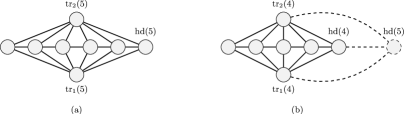
Figure 1. The graph $L_{5}$ and the construction of $L_{5}$ from $L_{4}$. $L_{5}$ is obtained from $L_{4}$ by adding the vertex $\mathrm{hd}(5)$ and its incident edges, and renaming $\mathrm{tr}_{1}(4)$ and $\mathrm{tr}_{2}(4)$ to $\mathrm{tr}_{1}(5)$ and $\mathrm{tr}_{2}(5)$ respectively.

Let $B\sqcup C$ be a partition of the set $\{\mathrm{tr}_{1},\mathrm{tr}_{2},\mathrm{hd}\}$. Let $B(h)$ be the subset of $\{\mathrm{tr}_{1}(h),\mathrm{tr}_{2}(h),\mathrm{hd}(h)\}$ which corresponds to $B$ and let $C(h)$ be defined similarly. We have that $B(h)$ and $C(h)$ form a partition of $\{\mathrm{tr}_{1}(h),\mathrm{tr}_{2}(h),\mathrm{hd}(h)\}$.

Definition 11.

We denote $b_{B,C}(h)=Z(L_{h};B(h),C(h);\mathsf{t},1)$.

The next two lemmas are devoted to computing $b_{B,C}(h)$.

Lemma 12.

$$b_{\{\mathrm{tr}_{1},\mathrm{hd}\},\{\mathrm{tr}_{2}\}}(h) = b_{\{\mathrm{tr}_{2},\mathrm{hd}\},\{\mathrm{tr}_{1}\}}(h)=$$

$$b_{\{\mathrm{tr}_{1}\},\{\mathrm{tr}_{2},\mathrm{hd}\}}(h) = b_{\{\mathrm{tr}_{2}\},\{\mathrm{tr}_{1},\mathrm{hd}\}}(h)=(\mathsf{t}^{2}+\mathsf{t})^{h}\cdot\mathsf{t}\,.$$

Proof.

We have

$$b_{\{\mathrm{tr}_{1},\mathrm{hd}\},\{\mathrm{tr}_{2}\}}(h) = b_{\{\mathrm{tr}_{2},\mathrm{hd}\},\{\mathrm{tr}_{1}\}}(h)=$$

$$b_{\{\mathrm{tr}_{1}\},\{\mathrm{tr}_{2},\mathrm{hd}\}}(h) = b_{\{\mathrm{tr}_{2}\},\{\mathrm{tr}_{1},\mathrm{hd}\}}(h)$$

by symmetry. We compute $b_{\{\mathrm{tr}_{1},\mathrm{hd}\},\{\mathrm{tr}_{2}\}}(h)$ by finding a simple linear recurrence relation which it satisfies and solving it. We divide the sum $b_{\{\mathrm{tr}_{1},\mathrm{hd}\},\{\mathrm{tr}_{2}\}}(h)$ into two sums,

$$b_{\{\mathrm{tr}_{1},\mathrm{hd}\},\{\mathrm{tr}_{2}\}}(h) = Z(L_{h};\{\mathrm{tr}_{1}(h),\mathrm{hd}(h),\mathrm{hd}(h-1)\},\{\mathrm{tr}_{2}(h)\};\mathsf{t},1)+$$

$$Z(L_{h};\{\mathrm{tr}_{1}(h),\mathrm{hd}(h)\},\{\mathrm{tr}_{2}(h),\mathrm{hd}(h-1)\};\mathsf{t},1)$$

depending on whether $\mathrm{hd}(h-1)$ is in the iteration variable $S$ of the sum $b_{\{\mathrm{tr}_{1},\mathrm{hd}\},\{\mathrm{tr}_{2}\}}(h)$ (as in Definition 6). These two sums can be obtained from $b_{\{\mathrm{tr}_{1},\mathrm{hd}\},\{\mathrm{tr}_{2}\}}(h-1)$ and $b_{\{\mathrm{tr}_{1}\},\{\mathrm{tr}_{2},\mathrm{hd}\}}(h-1)$ by adjusting for the addition of $\mathrm{hd}(h)$ and its incident edges:

• $\mathrm{hd}(h-1)\in S$: adding $\mathrm{hd}(h)$ (to the graph and to $S$) puts two new edges in $E(S)\sqcup E(\bar{S})$, namely $(\mathrm{tr}_{1},\mathrm{hd}(h))$ and $(\mathrm{hd}(h-1),\mathrm{hd}(h))$. Hence,

  $$Z(L_{h};\{\mathrm{tr}_{1}(h),\mathrm{hd}(h),\mathrm{hd}(h-1)\},\{\mathrm{tr}_{2}(h)\};\mathsf{t},1)$$

  $$=b_{\{\mathrm{tr}_{1},\mathrm{hd}\},\{\mathrm{tr}_{2}\}}(h-1)\cdot\mathsf{t}^{2}\,.$$

• $\mathrm{hd}(h-1)\notin S$: adding $\mathrm{hd}(h)$ puts just one new edge in $E(S)\sqcup E(\bar{S})$, namely $(\mathrm{tr}_{1},\mathrm{hd}(h))$. Hence,

  $$Z(L_{h};\{\mathrm{tr}_{1}(h),\mathrm{hd}(h)\},\{\mathrm{tr}_{2}(h),\mathrm{hd}(h-1)\};\mathsf{t},1)$$

  $$=b_{\{\mathrm{tr}_{1}\},\{\mathrm{tr}_{2},\mathrm{hd}\}}(h-1)\cdot\mathsf{t}\,.$$

Using that $b_{\{\mathrm{tr}_{1},\mathrm{hd}\},\{\mathrm{tr}_{2}\}}(h-1)=b_{\{\mathrm{tr}_{1}\},\{\mathrm{tr}_{2},\mathrm{hd}\}}(h-1)$, we get:

(2) $$b_{\{\mathrm{tr}_{1},\mathrm{hd}\},\{\mathrm{tr}_{2}\}}(h)=b_{\{\mathrm{tr}_{1},\mathrm{hd}\},\{\mathrm{tr}_{2}\}}(h-1)\cdot(\mathsf{t}^{2}+\mathsf{t})$$

and the lemma follows since $b_{\{\mathrm{tr}_{1},\mathrm{hd}\},\{\mathrm{tr}_{2}\}}(0)=\mathsf{t}$ (note $L_{0}$ is simply a path of length $3$). ∎

We are left with two distinct cases of $b_{B,C}(h)$ to compute, since by symmetry,

$$b_{\{\mathrm{tr}_{1},\mathrm{tr}_{2},\mathrm{hd}\},\emptyset}(h)=b_{\emptyset,\{\mathrm{tr}_{1},\mathrm{tr}_{2},\mathrm{hd}\}}(h)\mbox{ and }b_{\{\mathrm{tr}_{1},\mathrm{tr}_{2}\},\{\mathrm{hd}\}}(h)=b_{\{\mathrm{hd}\},\{\mathrm{tr}_{1},\mathrm{tr}_{2}\}}(h)\,.$$

Lemma 13.

Let

$$\lambda_{1,2}=\frac{\mathsf{t}}{2}\left(1+\mathsf{t}^{2}\pm\sqrt{5-2\mathsf{t}^{2}+\mathsf{t}^{4}}\right)\,,$$

$$c_{1}=\mathsf{t}^{2}-c_{2}\,,$$

$$c_{2}=\frac{\mathsf{t}\left(-\mathsf{t}^{3}-2+\mathsf{t}+\mathsf{t}\sqrt{5-2\mathsf{t}^{2}+\mathsf{t}^{4}}\right)}{2\sqrt{5-2\mathsf{t}^{2}+\mathsf{t}^{4}}}\,,$$

$$d_{1}=1-d_{2}\,,$$

$$d_{2}=\frac{-1-2\mathsf{t}+\mathsf{t}^{2}+\sqrt{5-2\mathsf{t}^{2}+\mathsf{t}^{4}}}{2\sqrt{5-2\mathsf{t}^{2}+\mathsf{t}^{4}}}\,.$$

$\lambda_{1}$ corresponds to the $+$ case. If $\mathsf{t}\in\mathbb{R}$ then $c_{1},c_{2},d_{1},d_{2},\lambda_{1},\lambda_{2}\in\mathbb{R}$, $\lambda_{1}\not=\lambda_{2}$, and

$$b_{\{\mathrm{tr}_{1},\mathrm{tr}_{2},\mathrm{hd}\},\emptyset}(h)=c_{1}\lambda_{1}^{h}+c_{2}\lambda_{2}^{h}$$

$$b_{\{\mathrm{tr}_{1},\mathrm{tr}_{2}\},\{\mathrm{hd}\}}(h)=d_{1}\lambda_{1}^{h}+d_{2}\lambda_{2}^{h}\,.$$

Proof.

The content of the square root is always strictly positive for $\mathsf{t}\in\mathbb{R}$. Hence, $\lambda_{1}\not=\lambda_{2}$ and $c_{1},c_{2},d_{1},d_{2},\lambda_{1},\lambda_{2}\in\mathbb{R}$.

The sequences $b_{\{\mathrm{tr}_{1},\mathrm{tr}_{2},\mathrm{hd}\},\emptyset}(h)$ and $b_{\{\mathrm{tr}_{1},\mathrm{tr}_{2}\},\{\mathrm{hd}\}}(h)$ satisfy a mutual linear recurrence as follows:

$$b_{\{\mathrm{tr}_{1},\mathrm{tr}_{2},\mathrm{hd}\},\emptyset}(h) = b_{\{\mathrm{tr}_{1},\mathrm{tr}_{2},\mathrm{hd}\},\emptyset}(h-1)\cdot\mathsf{t}^{3}+b_{\{\mathrm{tr}_{1},\mathrm{tr}_{2}\},\{\mathrm{hd}\}}(h-1)\cdot\mathsf{t}^{2}$$

$$b_{\{\mathrm{tr}_{1},\mathrm{tr}_{2}\},\{\mathrm{hd}\}}(h) = b_{\{\mathrm{tr}_{1},\mathrm{tr}_{2},\mathrm{hd}\},\emptyset}(h-1)+b_{\{\mathrm{tr}_{1},\mathrm{tr}_{2}\},\{\mathrm{hd}\}}(h-1)\cdot\mathsf{t}$$

This implies that both $b_{\{\mathrm{tr}_{1},\mathrm{tr}_{2},\mathrm{hd}\},\emptyset}(h)$ and $b_{\{\mathrm{tr}_{1},\mathrm{tr}_{2}\},\{\mathrm{hd}\}}(h)$ satisfy linear recurrence relations with the following initial conditions:

$$b_{\{\mathrm{tr}_{1},\mathrm{tr}_{2},\mathrm{hd}\},\emptyset}(0)=t^{2}\mbox{ and }b_{\{\mathrm{tr}_{1},\mathrm{tr}_{2},\mathrm{hd}\},\emptyset}(1)=t^{5}+t^{2}$$

$$b_{\{\mathrm{tr}_{1},\mathrm{tr}_{2}\},\{\mathrm{hd}\}}(0)=1\mbox{ and }b_{\{\mathrm{tr}_{1},\mathrm{tr}_{2}\},\{\mathrm{hd}\}}(1)=t^{2}+t\,.$$

These recurrences can be calculated and solved using standard methods, see e.g. [11] or [16]. ∎

Using the previous two lemmas, we get:

Lemma 14.

$$Z(L_{h};\{\mathrm{tr}_{1}\},\{\mathrm{tr}_{2}\};\mathsf{t},1) = Z(L_{h};\{\mathrm{tr}_{2}\},\{\mathrm{tr}_{1}\};\mathsf{t},1)=2\mathsf{t}(\mathsf{t}^{2}+\mathsf{t})^{h}$$

$$Z(L_{h};\{\mathrm{tr}_{1},\mathrm{tr}_{2}\},\emptyset;\mathsf{t},1) = Z(L_{h};\emptyset,\{\mathrm{tr}_{1},\mathrm{tr}_{2}\};\mathsf{t},1)=(c_{1}+d_{1})\lambda_{1}^{h}+(c_{2}+d_{2})\lambda_{2}^{h}\,,$$

where $c_{1},c_{2},d_{1},d_{2},\lambda_{1},\lambda_{2}$ are as in Lemma 13.

Proof.

The lemma follows from Lemmas 12 and 13. ∎

Definition 15 (Phi graphs).

Let $\mathcal{H}$ be a finite set of positive integers. We denote by $\Phi_{\mathcal{H}}$ the graph obtained from the disjoint union of the graphs $L_{h}:h\in\mathcal{H}$ as follows. For each $i=1,2$, the vertices $\mathrm{tr}_{i}(h)$, $h\in\mathcal{H}$, are identified into one vertex denoted $\mathrm{tr}_{i}(\mathcal{H})$.

The number of vertices in $\Phi_{\mathcal{H}}$ is $2+\sum_{h\in\mathcal{H}}(h+1)$. Figure 2 shows $\Phi_{\{1,3,4\}}$.

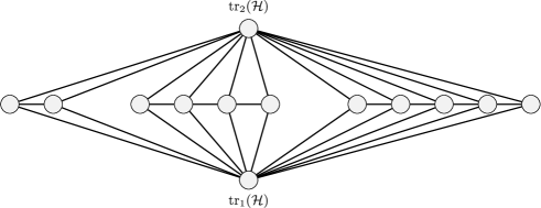
Figure 2. An example of a Phi graph: the graph $\Phi_{\mathcal{H}}$ for $\mathcal{H}=\{1,3,4\}$.

Lemma 16.

Let $\mathcal{H}$ be a finite set of positive integers. Then

$$Z(\Phi_{\mathcal{H}};\{\mathrm{tr}_{1}(\mathcal{H})\},\{\mathrm{tr}_{2}(\mathcal{H})\};\mathsf{t},1)=(2\mathsf{t})^{|\mathcal{H}|}\prod_{h\in\mathcal{H}}(\mathsf{t}^{2}+\mathsf{t})^{h}\,,$$

and

$$Z(\Phi_{\mathcal{H}};\{\mathrm{tr}_{1}(\mathcal{H}),\mathrm{tr}_{2}(\mathcal{H})\},\emptyset;\mathsf{t},1) =$$

$$Z(\Phi_{\mathcal{H}};\emptyset,\{\mathrm{tr}_{1}(\mathcal{H}),\mathrm{tr}_{2}(\mathcal{H})\};\mathsf{t},1) = \prod_{h\in\mathcal{H}}\left((c_{1}+d_{1})\lambda_{1}^{h}+(c_{2}+d_{2})\lambda_{2}^{h}\right)\,.$$

Proof.

It follows from Lemma 14 using that all edges are contained in some $L_{h}$. ∎

We can now define the graphs $G\otimes\mathcal{H}$:

Definition 17 ($G\otimes\mathcal{H}$).

Let $\mathcal{H}$ be a finite set of positive integers. Let $G$ be a graph. For every edge $e=(u_{1},u_{2})\in E(G)$, let $\Phi_{\mathcal{H},e}$ be a new copy of $\Phi_{\mathcal{H}}$, where we denote $\mathrm{tr}_{1}(\mathcal{H})$ and $\mathrm{tr}_{2}(\mathcal{H})$ for $\Phi_{\mathcal{H},e}$ by $\mathrm{tr}_{1}(\mathcal{H},e)$ and $\mathrm{tr}_{2}(\mathcal{H},e)$. Let $G\otimes\Phi_{\mathcal{H}}=G\otimes\mathcal{H}$ be the graph obtained from the disjoint union of the graphs

$$\Phi_{\mathcal{H},e}:e\in E(G)$$

by identifying $\mathrm{tr}_{i}(\mathcal{H},e)$ with $u_{i}$, $i=1,2$, for every edge $e=(u_{1},u_{2})\in E(G)$.

Lemma 18.

Let $\mathcal{H}$ be a finite set of positive integers. Let $f_{\mathsf{t},\mathcal{H}}$ and $g_{p,\mathcal{H}}$ be the following functions:

$$f_{\mathsf{t},\mathcal{H}}(e_{1},e_{2},r_{1},r_{2}) = \prod_{h\in\mathcal{H}}\left(e_{1}r_{1}^{h}+e_{2}r_{2}^{h}\right)$$

$$f_{p,\mathcal{H}}(\mathsf{t}) = \left((2\mathsf{t})^{|\mathcal{H}|}\prod_{h\in\mathcal{H}}(\mathsf{t}^{2}+\mathsf{t})^{h}\right)^{m_{G}}\,.$$

Then

$$Z(G\otimes\mathcal{H};\mathsf{t},1) = f_{p,\mathcal{H}}(\mathsf{t})\cdot Z\left(G;f_{\mathsf{t},\mathcal{H}}\left(\frac{c_{1}+d_{1}}{2t},\frac{c_{2}+d_{2}}{2t},\frac{\lambda_{1}}{\mathsf{t}^{2}+\mathsf{t}},\frac{\lambda_{2}}{\mathsf{t}^{2}+\mathsf{t}}\right),1\right)\,.$$

Proof.

Let $\tilde{G}=G\otimes\mathcal{H}$. By definition,

$$Z(\tilde{G};\mathsf{t},1)=\sum_{S\subseteq V(\tilde{G})}\mathsf{t}^{|E_{\tilde{G}}(S)\sqcup E_{\tilde{G}}(\bar{S})|}\,.$$

We can rewrite this sum as

$$Z(\tilde{G};\mathsf{t},1) = \sum_{S\subseteq V(G)}\left(\prod_{e\in[S,\bar{S}]_{G}}Z(\Phi_{\mathcal{H},e};\{\mathrm{tr}_{1}(\mathcal{H},e)\},\{\mathrm{tr}_{2}(\mathcal{H},e)\};\mathsf{t},1)\right)$$

$$\cdot\left(\prod_{e\in E_{G}(S)\sqcup E_{G}(\bar{S})}Z(\Phi_{\mathcal{H},e};\{\mathrm{tr}_{1}(\mathcal{H},e),\mathrm{tr}_{2}(\mathcal{H},e)\},\emptyset;\mathsf{t},1)\right)\,,$$

since edges only occur within some $\Phi_{\mathcal{H},e}$. Using lemma 16, the sum in the last equation can be written as

$$\sum_{S\subseteq V(G)}\left((2\mathsf{t})^{|\mathcal{H}|}\prod_{h\in\mathcal{H}}(\mathsf{t}^{2}+\mathsf{t})^{h}\right)^{|[S,\bar{S}]_{G}|}\cdot$$

$$\left(\prod_{h\in\mathcal{H}}\left((c_{1}+d_{1})\lambda_{1}^{h}+(c_{2}+d_{2})\lambda_{2}^{h}\right)\right)^{|E_{G}(S)\sqcup E_{G}(\bar{S})|}\,.$$

Since $|[S,\bar{S}]_{G}=m_{G}-|E_{G}(S)\sqcup E_{G}(\bar{S})|$, we can rewrite the last equation as

$$\left((2\mathsf{t})^{|\mathcal{H}|}\prod_{h\in\mathcal{H}}(\mathsf{t}^{2}+\mathsf{t})^{h}\right)^{m_{G}}\cdot$$

$$\sum_{S\subseteq V(G)}\left(\frac{\prod_{h\in\mathcal{H}}\left((c_{1}+d_{1})\lambda_{1}^{h}+(c_{2}+d_{2})\lambda_{2}^{h}\right)}{(2\mathsf{t})^{|\mathcal{H}|}\prod_{h\in\mathcal{H}}(\mathsf{t}^{2}+\mathsf{t})^{h}}\right)^{|E_{G}(S)\sqcup E_{G}(\bar{S})|}\,.$$

The last sum can be rewritten as

$$\sum_{S\subseteq V(G)}\left[\prod_{h\in\mathcal{H}}\left(\frac{c_{1}+d_{1}}{2t}\left(\frac{\lambda_{1}}{\mathsf{t}^{2}+\mathsf{t}}\right)^{h}+\frac{c_{2}+d_{2}}{2t}\left(\frac{\lambda_{2}}{\mathsf{t}^{2}+\mathsf{t}}\right)^{h}\right)\right]^{|E_{G}(S)\sqcup E_{G}(\bar{S})|}$$

and the lemma follows. ∎

The construction described above will be useful to deal with the evaluation of $Z(G;\mathsf{t},\mathsf{y})$ with $\mathsf{y}=-1$ due to the following lemma. For a graph $G$, let $G_{(1)}$ be the graph obtained from $G$ by adding, for each $v\in V(G)$, a new vertex $v^{\prime}$ and an edge $(v,v^{\prime})$. So $v^{\prime}$ is adjacent to $v$ only. $G_{(1)}$ is a graph with $2n_{G}$ vertices.

Lemma 19.

$Z(G;\mathsf{t},1)=(\mathsf{t}-1)^{-n_{G}}Z(G_{(1)};\mathsf{t},-1)$

Proof.

By definition we have

$$Z(G_{(1)};\mathsf{t},-1) = \sum_{S\subseteq V(G_{(1)})}\mathsf{t}^{|E_{G_{(1)}}(S)\sqcup E_{G_{(1)}}(\bar{S})|}(-1)^{|S|}$$

$$= \sum_{S\subseteq V(G)}\mathsf{t}^{|E_{G}(S)\sqcup E_{G}(\bar{S})|}(\mathsf{t}-1)^{|S|}(\mathsf{t}-1)^{n_{G}-|S|}$$

where the last equality is by considering the contribution of $v^{\prime}$ for each $v\in V(G)$: if $v\in S$ then $v^{\prime}$ contributes either $-\mathsf{t}$ or $1$; if $v\notin S$ then $v^{\prime}$ contributes either $\mathsf{t}$ or $-1$. The last expression in the equation above equals

$$(\mathsf{t}-1)^{n_{G}}\sum_{S\subseteq V(G)}\mathsf{t}^{|E_{G}(S)\sqcup E_{G}(\bar{S})|} = (\mathsf{t}-1)^{n_{G}}\cdot Z(G;\mathsf{t},1)\,.$$

∎

3.2. The Ising polynomials of certain trees

We denote be $S_{n}$ the star with $n$ leaves. Let $\mathrm{cent}(S_{n})$ be the central vertex of the star $S_{n}$. A construction based on stars will be used to interpolate the $\mathsf{y}$ indeterminate from $Z(G;\gamma,\delta)$. First, notice the following:

Proposition 20.

For every $n\in\mathbb{N}^{+}$,

$$Z(S_{n};\{\mathrm{cent}(S_{n})\},\emptyset;\mathsf{t},\mathsf{y}) = \mathsf{y}\cdot(\mathsf{y}\mathsf{t}+1)^{n}$$

$$Z(S_{n};\emptyset,\{\mathrm{cent}(S_{n})\};\mathsf{t},\mathsf{y}) = (\mathsf{y}+\mathsf{t})^{n}$$

Proof.

By definition,

$$Z(S_{n};\{\mathrm{cent}{S_{n}}\},\emptyset;\mathsf{t},\mathsf{y}) = \sum_{S:\{\mathrm{cent}(S_{n})\}\subseteq S\subseteq V(S_{n})}\mathsf{t}^{|E_{S_{n}}(S)\sqcup E_{S_{n}}(\bar{S})|}\mathsf{y}^{|S|}$$

$$Z(S_{n};\emptyset,\{\mathrm{cent}{S_{n}}\};\mathsf{t},\mathsf{y}) = \sum_{S\subseteq V(S_{n})\setminus\{\mathrm{cent}(S_{n})\}}\mathsf{t}^{|E_{S_{n}}(S)\sqcup E_{S_{n}}(\bar{S})|}\mathsf{y}^{|S|}$$

Consider a leaf $v$ of $S_{n}$. For $Z(S_{n};\{\mathrm{cent}(S_{n})\},\emptyset;\mathsf{t},\mathsf{y})$, a leaf $v$ has two options: either $v\in S$, in which case it contributes the weight of its incident edge, so its contribution is $\mathsf{y}\mathsf{t}$; or $v\not\in S$, in which case it contributes $1$. For $Z(S_{n};\emptyset,\{\mathrm{cent}(S_{n})\};\mathsf{t},\mathsf{y})$, $v$ has two options: either $v\in S$, in which case it does not contribute the weight of its edge, so its contribution is $\mathsf{y}$; or $v\not\in S$, in which case its edge contributes $\mathsf{t}$. ∎

Definition 21 (The graph $S_{\mathcal{H}}$).

Let $\mathcal{H}$ be a set of positive integers. The graph $S_{\mathcal{H}}$ is obtained from the disjoint union of $S_{n}:n\in\mathcal{H}$ and a new vertex $\mathrm{cent}(\mathcal{H})$ by adding edges between $\mathrm{cent}(\mathcal{H})$ and the centers $\mathrm{cent}(S_{n})$ of all the stars $S_{n}:n\in\mathcal{H}$.

See Figure 3(a) for an example.

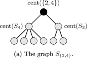
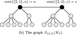
Figure 3. Examples of $S_{\mathcal{H}}$ and $S_{\mathcal{H}}(G)$. In (b), the black vertices $u,v$ are the vertices of $K_{2}$. They are also denoted $\mathrm{cent}(\mathcal{H},u)$ and $\mathrm{cent}(\mathcal{H},v)$ respectively.

Proposition 22.

Let $\mathcal{H}$ be a set of positive integers. Then,

$$Z(S_{\mathcal{H}};\{\mathrm{cent}(\mathcal{H})\},\emptyset;\mathsf{t},\mathsf{y}) =\mathsf{y}\cdot\displaystyle{\prod_{h\in\mathcal{H}}} \big{(}\mathsf{y}\mathsf{t}\cdot(\mathsf{y}\mathsf{t}+1)^{h}+(\mathsf{y}+\mathsf{t})^{h}\big{)}$$

$$Z(S_{\mathcal{H}};\emptyset,\{\mathrm{cent}(\mathcal{H})\};\mathsf{t},\mathsf{y}) =\displaystyle{\prod_{h\in\mathcal{H}}} \big{(}\mathsf{y}\cdot(\mathsf{y}\mathsf{t}+1)^{h}+\mathsf{t}\cdot(\mathsf{y}+\mathsf{t})^{h}\big{)}$$

Proof.

We have

$$Z(S_{\mathcal{H}};\{\mathrm{cent}(\mathcal{H})\},\emptyset;\mathsf{t},\mathsf{y}) =\mathsf{y}\cdot\displaystyle{\prod_{h\in\mathcal{H}}} \big{(}\mathsf{t}\cdot Z(S_{h};\{\mathrm{cent}(S_{h})\},\emptyset;\mathsf{t},\mathsf{y})$$

$$\ +Z(S_{h};\emptyset,\{\mathrm{cent}(S_{h})\};\mathsf{t},\mathsf{y})\big{)}$$

$$Z(S_{\mathcal{H}};\emptyset,\{\mathrm{cent}(\mathcal{H})\};\mathsf{t},\mathsf{y}) =\displaystyle{\prod_{h\in\mathcal{H}}} \big{(}Z(S_{h};\{\mathrm{cent}(S_{h})\},\emptyset;\mathsf{t},\mathsf{y})$$

$$\ +\mathsf{t}\cdot Z(S_{h};\emptyset,\{\mathrm{cent}(S_{h})\};\mathsf{t},\mathsf{y})\big{)}$$

and by Proposition 20, the claim follows. ∎

Definition 23 (The graph $S_{\mathcal{H}}(G)$).

Let $\mathcal{H}$ be a set of positive integers and let $G$ be a graph. For every vertex $v$ of $G$, let $S_{\mathcal{H},v}(G)$ be a new copy of $S_{\mathcal{H}}$. We denote the center of each such copy of $S_{\mathcal{H}}$ by $\mathrm{cent}(\mathcal{H},v)$. Let $S_{\mathcal{H}}(G)$ be the graph obtained from the disjoint union of the graphs in the set

$$\{G\}\cup\{S_{\mathcal{H},v}:v\in V(G)\}$$

by identifying the pairs of vertices $v$ and $\mathrm{cent}(\mathcal{H},v)$.

In other words, $S_{\mathcal{H}}(G)$ is the rooted product of $G$ and $\left(S_{\mathcal{H}},\mathrm{cent}(\mathcal{H})\right)$. See Figure 3(b) for an example.

Proposition 24.

Let $\mathcal{H}$ be a set of positive integers. Let

$$g_{p,\mathcal{H}}(\mathsf{t},\mathsf{y}) = \left(\displaystyle{\prod_{h\in\mathcal{H}}}\big{(}\mathsf{y}\cdot(\mathsf{y}\mathsf{t}+1)^{h}+\mathsf{t}\cdot(\mathsf{y}+\mathsf{t})^{h}\big{)}\right)^{|V(G)}$$

$$g_{\mathsf{y},\mathcal{H}}(\mathsf{t},\mathsf{y}) = \mathsf{y}\displaystyle{\prod_{h\in\mathcal{H}}}\frac{\mathsf{y}\mathsf{t}\cdot(\mathsf{y}\mathsf{t}+1)^{h}+(\mathsf{y}+\mathsf{t})^{h}}{\mathsf{y}\cdot(\mathsf{y}\mathsf{t}+1)^{h}+\mathsf{t}\cdot(\mathsf{y}+\mathsf{t})^{h}}$$

Then

$$Z(S_{\mathcal{H}}(G);\mathsf{t},\mathsf{y})=g_{p,\mathcal{H}}(\mathsf{t},\mathsf{y})\cdot Z(G;\mathsf{t},g_{\mathsf{y},\mathcal{H}}(\mathsf{t},\mathsf{y}))\,.$$

Proof.

By definition

$$Z(S_{\mathcal{H}}(G);\mathsf{t},\mathsf{y})=\sum_{S\subseteq V(S_{\mathcal{H}}(G))}\mathsf{t}^{|E_{S_{\mathcal{H}}(G)}(S)\sqcup E_{S_{\mathcal{H}}(G)}(\bar{S})|}\mathsf{y}^{|S|}\,.$$

We would like to rewrite this sum as a sum over $S\subseteq V(G)$. By the structure of $S_{\mathcal{H}}(G)$,

$$Z(S_{\mathcal{H}}(G);\mathsf{t},\mathsf{y}) = \sum_{S\subseteq V(G)}\mathsf{t}^{|E_{G}(S)\sqcup E_{G}(\bar{S})|}$$

$$\left(\prod_{v\in S}Z(S_{\mathcal{H},v};\{\mathrm{cent}(\mathcal{H},v)\},\emptyset;\mathsf{t},\mathsf{y})+\right.$$

$$\ \ \left.\prod_{v\in\bar{S}}Z(S_{\mathcal{H},v};\emptyset,\{\mathrm{cent}(\mathcal{H},v)\};\mathsf{t},\mathsf{y})\right)$$

By Proposition 22,

$$Z(S_{\mathcal{H}}(G);\mathsf{t},\mathsf{y}) = \sum_{S\subseteq V(G)}\mathsf{t}^{|E_{G}(S)\sqcup E_{G}(\bar{S})|}$$

$$\left(\left(\mathsf{y}\cdot\displaystyle{\prod_{h\in\mathcal{H}}}\big{(}\mathsf{y}\mathsf{t}\cdot(\mathsf{y}\mathsf{t}+1)^{h}+(\mathsf{y}+\mathsf{t})^{h}\big{)}\right)^{|S|}\right.$$

$$\ \ \left.\left(\displaystyle{\prod_{h\in\mathcal{H}}}\big{(}\mathsf{y}\cdot(\mathsf{y}\mathsf{t}+1)^{h}+\mathsf{t}\cdot(\mathsf{y}+\mathsf{t})^{h}\big{)}\right)^{|V(G)\setminus|S|}\right)$$

and the claim follows.

∎

The following propositions will be useful:

Proposition 25.

Let $g_{\mathsf{y},\mathcal{H}}(\mathsf{t},\mathsf{y})$ be as in Proposition 24. Let $h_{\mathsf{y},\mathcal{H}}$ be the function given by

$$h_{\mathsf{y},\mathcal{H}}(e_{1},e_{2},r)=\displaystyle{\prod_{h\in\mathcal{H}}}\left(1+\frac{1}{e_{1}+e_{2}\cdot r^{h}}\right)\,.$$

Let $\gamma,\delta\notin\{-1,0,1\}$ such that $\gamma\not=-\delta$. There exist constants $h_{1},u_{1},u_{2},w$ (which depend on $\gamma$ and $\delta$) such that for every two finite sets of positive even numbers $\mathcal{H}_{1}$ and $\mathcal{H}_{2}$ which satisfy

• $|\mathcal{H}_{1}|=|\mathcal{H}_{2}|$, and $\mathcal{H}_{1},\mathcal{H}_{2}\subseteq\mathbb{N}^{+}\setminus\{1,\ldots,h_{1}\}$,

we have

1. $g_{\mathsf{y},\mathcal{H}_{1}}(\gamma,\delta),g_{\mathsf{y},\mathcal{H}_{1}}(\gamma,\delta),h_{\mathsf{y},\mathcal{H}_{1}}(u_{1},u_{2},w),h_{\mathsf{y},\mathcal{H}_{2}}(u_{1},u_{2},w)\in\mathbb{R}\setminus\{0\}$, and

2. $g_{\mathsf{y},\mathcal{H}_{1}}(\gamma,\delta)=g_{\mathsf{y},\mathcal{H}_{2}}(\gamma,\delta)$ iff $h_{\mathsf{y},\mathcal{H}_{1}}(u_{1},u_{2},w)=h_{\mathsf{y},\mathcal{H}_{2}}(u_{1},u_{2},w)$

Furthermore, $u_{1}$ and $u_{2}$ are non-zero and $w\notin\{-1,0,1\}$.

Proof.

It cannot hold that $|\delta\gamma+1|=|\delta+\gamma|$. Furthermore we know that $\gamma,\delta\not=0$. Hence, there is $h_{1}$ such that for every even $h>h_{1}$,the sequences $\delta(\delta\gamma+1)^{h}+\gamma\cdot(\delta+\gamma)^{h}$ and $\delta\gamma(\delta\gamma+1)^{h}+(\delta+\gamma)^{h}$ are strictly ascending or descending, and in particular, are non-zero. Therefore we have $g_{\mathsf{y},\mathcal{H}_{1}}(\gamma,\delta),g_{\mathsf{y},\mathcal{H}_{1}}(\gamma,\delta)\in\mathbb{R}\setminus\{0\}$.

We have for $i=1,2$

$$g_{\mathsf{y},\mathcal{H}_{i}}(\gamma,\delta) = \delta\displaystyle{\prod_{h\in\mathcal{H}_{i}}}\frac{\delta\gamma\cdot(\delta\gamma+1)^{h}+(\delta+\gamma)^{h}}{\delta(\delta\gamma+1)^{h}+\gamma\cdot(\delta+\gamma)^{h}}$$

$$= \frac{\delta}{\gamma^{|\mathcal{H}_{i}|}}\displaystyle{\prod_{h\in\mathcal{H}_{i}}}\frac{\delta\gamma^{2}\cdot(\delta\gamma+1)^{h}+\gamma\cdot(\delta+\gamma)^{h}}{\delta(\delta\gamma+1)^{h}+\gamma\cdot(\delta+\gamma)^{h}}$$

$$= \frac{\delta}{\gamma^{|\mathcal{H}_{i}|}}\displaystyle{\prod_{h\in\mathcal{H}_{i}}}\left(1+\frac{\delta(\gamma^{2}-1)\cdot(\delta\gamma+1)^{h}}{\delta(\delta\gamma+1)^{h}+\gamma\cdot(\delta+\gamma)^{h}}\right)$$

$$= \frac{\delta}{\gamma^{|\mathcal{H}_{i}|}}\displaystyle{\prod_{h\in\mathcal{H}_{i}}}\left(1+\frac{1}{\frac{1}{\gamma^{2}-1}+\frac{\gamma}{\delta(\gamma^{2}-1)}\cdot\left(\frac{\delta+\gamma}{\delta\gamma+1}\right)^{h}}\right)$$

Let $u_{1}=\frac{1}{\gamma^{2}-1}$, $u_{2}=\frac{\gamma}{\delta(\gamma^{2}-1)}$ and $w=\frac{\delta+\gamma}{\delta\gamma+1}$. We have $u_{1},u_{2},w\in\mathbb{R}\setminus\{0\}$ and $w\notin\{-1,1\}$. Hence, we can take $h_{1}$ to be large enough so that $u_{1}+u_{2}+w^{h}$ non-zero. Since $u_{1}+u_{2}+w^{h}$ is strictly ascending or descending for even $h$, we have $h_{\mathsf{y},\mathcal{H}_{1}}(u_{1},u_{2},w),h_{\mathsf{y},\mathcal{H}_{2}}(u_{1},u_{2},w)\in\mathbb{R}\setminus\{0\}$ for large enough values of $h$. ∎

Proposition 26.

Let $\gamma,\delta\notin\{-1,0,1\}$ and $\gamma\not=-\delta$. Let $\mathcal{H}$ be a set of positive even integers. Let $g_{p,\mathcal{H}}(\mathsf{t},\mathsf{y}))$ be from Proposition 24. Then there exists $h_{2}$ such that if $\mathcal{H}\subseteq\mathbb{N}^{+}\setminus\{1,\ldots,h_{2}\}$ then $g_{p,\mathcal{H}}(\gamma,\delta))\not=0$.

Proof.

Recall

$$g_{p,\mathcal{H}}(\gamma,\delta))=\left(\displaystyle{\prod_{h\in\mathcal{H}}}\big{(}\delta(\delta\gamma+1)^{h}+\gamma\cdot(\delta+\gamma)^{h}\big{)}\right)^{|V(G)|}\,.$$

We have that $\delta+\gamma$ is non-zero. If $\delta\gamma+1=0$ then the claim holds even for $h_{2}=0$. Otherwise, using that $|\delta\gamma+1|\not=|\delta+\gamma|$, at least one of $(\delta\gamma+1)^{h},(\delta+\gamma)^{h}$ becomes strictly larger in absolute value than the other for large enough $h$. ∎

3.3. Proof of Theorem 1

The following lemma is a variation of Lemma 4 in [7].

For any $\mathcal{H}$, let $\sigma(\mathcal{H})={\sum_{h\in\mathcal{H}}h}$.

Lemma 27.

Let $\gamma\notin\{-1,0,1\}$, $\delta\not=0$, $e_{1},e_{2}\not=0$ and $r_{1},r_{2}\notin\{-1,0,1\}$ such that $|r_{1}|\not=|r_{2}|$. For every positive integer $q^{\prime}$ there exist $\hat{q}=\Omega(q^{\prime})$ sets of positive even integers $\mathcal{H}_{0},\ldots,\mathcal{H}_{\hat{q}}$ such that

1. $\sigma(\mathcal{H}_{i})=O(\log^{3}q^{\prime})$ for all $i$,

2. $\sigma(\mathcal{H}_{i})=\sigma(\mathcal{H}_{j})$ for all $i\not=j$,

3. $f_{\mathsf{t},\mathcal{H}_{i}}(e_{1},e_{2},r_{1},r_{2})\not=f_{\mathsf{t},\mathcal{H}_{j}}(e_{1},e_{2},r_{1},r_{2})$ for $i\not=j$,

where $f_{\mathsf{t},\mathcal{H}}(e_{1},e_{2},r_{1},r_{2})$ is from Proposition 18. If additionally $\delta\notin\{-1,1\}$ and $\gamma\not=-\delta$, we have

1. $g_{\mathsf{y},\mathcal{H}_{i}}(\gamma,\delta)\not=g_{\mathsf{y},\mathcal{H}_{j}}(\gamma,\delta)$ for $i\not=j$.

2. $g_{p,\mathcal{H}_{i}}(\gamma,\delta)\not=0$,

where $g_{\mathsf{y},\mathcal{H}}(e_{1},e_{2},r_{1})$ is from Proposition 24.

The sets $\mathcal{H}_{i}$ can be computed in polynomial time in $q^{\prime}$.

Proof.

Let $q=q^{\prime}\log^{3}q^{\prime}$. First we define sets $\mathcal{H}_{0}^{\prime},\ldots,\mathcal{H}_{q}^{\prime}$. We will use these sets to define the desired sets $\mathcal{H}_{0},\ldots,\mathcal{H}_{\hat{q}}$.

For $i=0,\ldots,q$, let $i[0],\ldots,i[\ell]\in\{0,1\}$ be the binary expansion of $i$ where $\ell=\lfloor\log q\rfloor$. Let $\Delta$ be a positive even integer to be chosen later. Let $\tau\in\{1,2\}$ be such that $|r_{\tau}|=\max\{|r_{1}|,|r_{2}|\}$. Then $|r_{{3-\tau}}|=\min\{|r_{1}|,|r_{2}|\}$. Let $m_{0}$ be an even integer such that $m_{0}>h_{1}$ from Proposition 25 and $m_{0}>h_{2}$ from Proposition 26. We choose $\mathcal{H}_{i}^{\prime}$ as follows:

$$\mathcal{H}_{i}^{\prime}=\{m_{0}+\Delta\lceil\log q\rceil\cdot(2j+i[j]):0\leq j\leq\ell\}\,.$$

The sets $\mathcal{H}_{i}^{\prime}$ satisfy:

1. they are distinct,

2. they have equal cardinality $\ell$+1,

3. they contain only positive even integers between $m_{0}$
   and $m_{0}+\Delta(\log q+1)(2\log q+1)$, and

4. for $i,j$ and any $a\in\mathcal{H}_{i}^{\prime}$ and $b\in\mathcal{H}_{j}^{\prime}$, either $a=b$ or
   $|a-b|\geq\Delta\log q$.

It is easy to see that $\sigma(\mathcal{H}_{i}^{\prime})=\Omega(\log q)$, $i=0,\ldots,q$. On the other hand, since all the numbers in each of the $\mathcal{H}_{i}^{\prime}$ are bounded by $O(\log^{2}q)$ and the size of each $\mathcal{H}_{i}^{\prime}$ is $O(\log q)$, we get that $\sigma(\mathcal{H}_{i}^{\prime})=O(\log^{3}q)$ for each $i$. From this we get that at least $\hat{q}=\Omega\left(\frac{q^{\prime}\log^{3}q^{\prime}+1}{\log^{3}q^{\prime}}\right)=\Omega(q^{\prime})$ of the sets $\mathcal{H}_{0}^{\prime},\ldots,\mathcal{H}_{q}^{\prime}$ have the same sum value $\sigma(\mathcal{H}_{i}^{\prime})$. Let $\{\mathcal{H}_{0},\ldots,\mathcal{H}_{\hat{q}}\}$ be a subset of $\{\mathcal{H}_{0}^{\prime},\ldots,\mathcal{H}_{q}^{\prime}\}$ such that all the sets in $\{\mathcal{H}_{0},\ldots,\mathcal{H}_{\hat{q}}\}$ have the same sum value $\sigma(\mathcal{H}_{i})$. We have (i), (ii) and (v) for $\mathcal{H}_{0},\ldots,\mathcal{H}_{\hat{q}}$.

We now turn to (iii) and (iv). The proofs of (iii) and (iv) are similar but not identical.

Let $0\leq i\not=j\leq\hat{q}$, $\mathcal{H}_{i\setminus j}=\mathcal{H}_{i}\setminus\mathcal{H}_{j}$ and $\mathcal{H}_{j\setminus i}=\mathcal{H}_{j}\setminus\mathcal{H}_{i}$. Notice $\mathcal{H}_{i\setminus j}\cap\mathcal{H}_{j\setminus i}=\emptyset$.
Let $\sigma=\sigma(\mathcal{H}_{i\setminus j})=\sigma(\mathcal{H}_{j\setminus i})$ and let $d=|\mathcal{H}_{i\setminus j}|=|\mathcal{H}_{j\setminus i}|$.

1. We write $f_{\mathsf{t},\mathcal{H}_{i}}$ for short instead of $f_{\mathsf{t},\mathcal{H}_{i}}(e_{1},e_{2},r_{1},r_{2})$ in this proof. When other parameters are used instead of $e_{1},e_{2},r_{1},r_{2}$ we write them explicitly. Since $f_{\mathsf{t},\mathcal{H}_{i}}=f_{\mathsf{t},\mathcal{H}_{i\setminus j}}\cdot f_{\mathsf{t},\mathcal{H}_{i}\cap\mathcal{H}_{j}}$, $f_{\mathsf{t},\mathcal{H}_{j}}=f_{\mathsf{t},\mathcal{H}_{j\setminus i}}\cdot f_{\mathsf{t},\mathcal{H}_{i}\cap\mathcal{H}_{j}}$ and $f_{\mathsf{t},\mathcal{H}_{i}\cap\mathcal{H}_{j}}\not=0$, it is enough to show that $f_{\mathsf{t},\mathcal{H}_{i\setminus j}}-f_{\mathsf{t},\mathcal{H}_{j\setminus i}}\not=0$.

   Since $\sigma(\mathcal{H}_{i\setminus j})=\sigma(\mathcal{H}_{j\setminus i})$ we have

   $$f_{\mathsf{t},\mathcal{H}_{i\setminus j}}=f_{\mathsf{t},\mathcal{H}_{j\setminus i}}\mbox{ iff }f_{\mathsf{t},\mathcal{H}_{i\setminus j}}(e_{1},e_{2},r_{2}^{-1},r_{1}^{-1})=f_{\mathsf{t},\mathcal{H}_{j\setminus i}}(e_{1},e_{2},r_{2}^{-1},r_{1}^{-1})\,.$$

   Hence we can assume from now on that $|r_{\tau}|>1$ (otherwise we look at $r_{1}^{-1}$ and $r_{2}^{-1}$ instead).

   For every $\mathcal{H}$, $f_{\mathsf{t},\mathcal{H}}$ can be rewritten as follows:

   $$f_{\mathsf{t},\mathcal{H}}=\prod_{h\in\mathcal{H}}(e_{\tau}r_{\tau}^{h}+e_{3-\tau}r_{{3-\tau}}^{h})=e_{3-\tau}^{\ell+1}\sum_{X\subseteq\mathcal{H}}s_{\mathcal{H}}(X)\,,$$

   where

   $$s_{\mathcal{H}}(X)=\left(\frac{e_{\tau}}{e_{3-\tau}}\right)^{|X|}r_{\tau}^{\sigma(X)}r_{3-\tau}^{\sigma(\mathcal{H}\setminus X)}\,.$$

   We think of $h\in X$ (respectively $h\in\mathcal{H}\setminus X)$ as corresponding to $e_{\tau}r_{\tau}^{h}$ (respectively $e_{3-\tau}r_{3-\tau}^{h}$).

   It suffices to show that

   (3) $$\sum_{X_{1}\subseteq\mathcal{H}_{i\setminus j}}s_{\mathcal{H}_{i\setminus j}}(X)-\sum_{X_{2}\subseteq\mathcal{H}_{j\setminus i}}s_{\mathcal{H}_{j\setminus i}}(X)\not=0\,.$$

   It holds that $s_{\mathcal{H}_{i\setminus j}}(\mathcal{H}_{i\setminus j})=s_{\mathcal{H}_{j\setminus i}}(\mathcal{H}_{j\setminus i})=\left(\frac{e_{\tau}}{e_{3-\tau}}\right)^{\ell+1}r_{\tau}^{\sigma}$. Hence, $s_{\mathcal{H}_{i\setminus j}}(\mathcal{H}_{i\setminus j})$ and $s_{\mathcal{H}_{j\setminus i}}(\mathcal{H}_{j\setminus i})$ cancel out in Inequality (3). Similarly, $s_{\mathcal{H}_{i\setminus j}}(\emptyset)=s_{\mathcal{H}_{j\setminus i}}(\emptyset)=r_{{3-\tau}}^{\sigma}$ cancel out. Let $m_{1}$ be the minimal element in $\mathcal{H}_{i\setminus j}\sqcup\mathcal{H}_{j\setminus i}$. Without loss of generality, assume $m_{1}\in\mathcal{H}_{i\setminus j}$. We have

   $$s_{\mathcal{H}_{i\setminus j}}(\mathcal{H}_{i\setminus j}\setminus\{m_{1}\})=\left(\frac{e_{\tau}}{e_{3-\tau}}\right)^{\ell}r_{\tau}^{\sigma-m_{1}}r_{3-\tau}^{m_{1}}\,.$$

   $s_{\mathcal{H}_{i\setminus j}}(\mathcal{H}_{i\setminus j}\setminus\{m_{1}\})$ has the largest exponent of $r_{\tau}$ out of all the monomials in both of the sums in Inequality (3), and any other exponent of $r_{\tau}$ is smaller by at least $\Delta\log q$. We will show that Inequality (3) holds by showing the following:

   (4) $$|s_{\mathcal{H}_{i\setminus j}}(\mathcal{H}_{i\setminus j}\setminus\{m_{1}\})|>\sum_{X\subsetneq\mathcal{H}_{i\setminus j}\setminus\{m_{1}\}}|s_{\mathcal{H}_{i\setminus j}}(X)|+\sum_{X\subsetneq\mathcal{H}_{j\setminus i}}|s_{\mathcal{H}_{j\setminus i}}(X)|\,.$$

   Each of the sums in Inequality (4) has at most $2^{\log q+1}=2q$ monomials corresponding to the subsets of $\mathcal{H}_{i\setminus j}$ and $\mathcal{H}_{j\setminus i}$ respectively. The absolute value of each of these monomials can be bounded from above by $s\cdot|r_{\tau}|^{\sigma-m_{1}-\Delta\log q}|r_{3-\tau}|^{m_{1}+\Delta\log q}$, where $s$ is the maximum of $\left|\frac{e_{\tau}}{e_{3-\tau}}\right|^{\ell}$ and $1$. Hence, the right-hand side of Inequality (4) is at most

   $$4q\cdot s|r_{\tau}|^{\sigma-m_{1}-\Delta\log q}|r_{3-\tau}|^{m_{1}+\Delta\log q}=$$

   $$4qs\left(\frac{e_{\tau}}{e_{3-\tau}}\right)^{-\ell}\cdot\left|\frac{r_{3-\tau}}{r_{\tau}}\right|^{\Delta\log q}|s_{\mathcal{H}_{i\setminus j}}(\mathcal{H}_{i\setminus j}-\{m_{1}\})|\,.$$

   There exists a number $\Delta^{\prime}$ which does not depend on $q$ such that$4qs\left(\frac{e_{\tau}}{e_{3-\tau}}\right)^{-\ell}<(\Delta^{\prime})^{\log q}$ and (iii) follows by setting $\Delta$ large enough so that $\Delta^{\prime}\cdot\left|\frac{r_{3-\tau}}{r_{\tau}}\right|^{\Delta}<1$.

2. By Proposition 25, there exist $u_{1},u_{2}\not=0$ and $w\notin\{-1,0,1\}$ depending on $\gamma,\delta$ for which it is enough to show that $h_{\mathsf{y},\mathcal{H}_{i}}(u_{1},u_{2},w)\not=h_{\mathsf{y},\mathcal{H}_{j}}(u_{1},u_{2},w)$ to get (iv). We write $h_{\mathsf{y},\mathcal{H}_{i}}$ for short instead of $h_{\mathsf{y},\mathcal{H}_{i}}(u_{1},u_{2},w)$ in this proof.

   Since we have $h_{\mathsf{y},\mathcal{H}_{i}}=h_{\mathsf{y},\mathcal{H}_{i\setminus j}}\cdot h_{\mathsf{y},\mathcal{H}_{i}\cap\mathcal{H}_{j}}$, $h_{\mathsf{y},\mathcal{H}_{j}}=h_{\mathsf{y},\mathcal{H}_{j\setminus i}}\cdot h_{\mathsf{y},\mathcal{H}_{i}\cap\mathcal{H}_{j}}$ and $h_{\mathsf{y},\mathcal{H}_{i}\cap\mathcal{H}_{j}}\not=0$, it is enough to show that

   $$h_{\mathsf{y},\mathcal{H}_{i\setminus j}}-h_{\mathsf{y},\mathcal{H}_{j\setminus i}}\not=0\,,$$

   i.e.

   $${\prod_{h\in\mathcal{H}_{i\setminus j}}}\left(1+\frac{1}{u_{1}+u_{2}\cdot w^{h}}\right)-\displaystyle{\prod_{h\in\mathcal{H}_{j\setminus i}}}\left(1+\frac{1}{u_{1}+u_{2}\cdot w^{h}}\right)\not=0\,.$$

   or equivalently,

   (5) $$\displaystyle{\prod_{h\in\mathcal{H}_{i\setminus j}}}\left(u_{1}+u_{2}\cdot w^{h}+1\right)\prod_{h\in\mathcal{H}_{j\setminus i}}\left(u_{1}+u_{2}\cdot w^{h}\right) -$$

   $$\displaystyle{\prod_{h\in\mathcal{H}_{j\setminus i}}}\left(u_{1}+u_{2}\cdot w^{h}+1\right)\prod_{h\in\mathcal{H}_{i\setminus j}}\left(u_{1}+u_{2}\cdot w^{h}\right) \not= 0$$

   Consider a product of the form found in Inequality (5).

   $$\displaystyle{\prod_{h\in\mathcal{H}_{a}}}\left(u_{1}+u_{2}\cdot w^{h}+1\right)\prod_{h\in\mathcal{H}_{b}}\left(u_{1}+u_{2}\cdot w^{h}\right) =$$

   $$\sum_{X\subseteq\mathcal{H}_{a}\cup\mathcal{H}_{b}}(u_{1}+1)^{|\mathcal{H}_{a}\setminus X|}u_{1}^{|\mathcal{H}_{b}\setminus X|}w^{\sigma(X)}u_{2}^{|X|}$$

   Let

   $$p(X) = \left((u_{1}+1)^{|\mathcal{H}_{i\setminus j}\setminus X|}u_{1}^{|\mathcal{H}_{j\setminus i}\setminus X|}-(u_{1}+1)^{|\mathcal{H}_{j\setminus i}\setminus X|}u_{1}^{|\mathcal{H}_{i\setminus j}\setminus X|}\right)$$

   $$\cdot u_{2}^{|X|}w^{\sigma(X)}$$

   It suffices to show that

   (6) $$\sum_{X\subseteq\mathcal{H}_{i\setminus j}\cup\mathcal{H}_{j\setminus i}}p(X)\not=0\,.$$

   We have $p(\emptyset)=p(\mathcal{H}_{i\setminus j}\sqcup\mathcal{H}_{j\setminus i})=0$, using that $|\mathcal{H}_{i\setminus j}|=|\mathcal{H}_{j\setminus i}|$. Let $m_{1}$ be the minimal element in $\mathcal{H}_{i\setminus j}\sqcup\mathcal{H}_{j\setminus i}$. Without loss of generality, assume $m_{1}\in\mathcal{H}_{i\setminus j}$. We have

   $$\left|p(\mathcal{H}_{i\setminus j}\sqcup\mathcal{H}_{j\setminus i}-\{m_{1}\})\right| = \left|u_{2}^{2d-1}w^{2\sigma-m_{1}}\right|$$

   $$\left|p(\{m_{1}\})\right| = \left|((u_{1}+1)u_{1})^{d-1}u_{2}w^{m_{1}}\right|$$

   The largest exponent of $w$ in Inequality (6) is $w^{2\sigma-m_{1}}$. For all other monomials in (6), the power of $w$ is smaller by at least $\Delta\log q$. Similarly, the smallest exponent of $w$ in Inequality (6) is $w^{m_{1}}$. For all other monomials in (6), the power of $w$ is larger by at least $\Delta\log q$.

   Let $X_{0}\subseteq\mathcal{H}_{i\setminus j}\sqcup\mathcal{H}_{j\setminus i})$ be maximal with respect to $|p(X_{0})|$. Since $d\leq\log q+1$, we can choose $\Delta$ large enough so that we have $X_{0}=\mathcal{H}_{i\setminus j}\sqcup\mathcal{H}_{j\setminus i}-\{m_{1}\}$ if $|w|>1$ and $X_{0}=\{m_{1}\}$ if $|w|<1$.

   We have the following:

   (7) $$\left|\sum_{X\subseteq\mathcal{H}_{i\setminus j}\sqcup\mathcal{H}_{j\setminus i}:X\not=X_{0}}p(X)\right|<|p(X_{0})|$$

   implying that Inequality (6) holds. To see that Inequality (7) holds, note that

   $$\left|\sum_{\begin{subarray}{c}X\subseteq\mathcal{H}_{i\setminus j}\sqcup\mathcal{H}_{j\setminus i}:\\ X\not=X_{0}\end{subarray}}p(X)\right|\leq 2^{2\log q+2}\max_{X\subseteq\mathcal{H}_{i\setminus j}\sqcup\mathcal{H}_{j\setminus i}:X\not=X_{0}}|p(X)|$$

   Let

   $$k(d)=\max\left(\left|(u_{1}+1)^{d}\right|,1\right)\cdot\max\left(\left|u_{1}^{d}\right|,1\right)\cdot\max\left(\left|u_{2}^{d}\right|,1\right)\,.$$

   Then

   $$\left|\sum_{\begin{subarray}{c}X\subseteq\mathcal{H}_{i\setminus j}\sqcup\mathcal{H}_{j\setminus i}:\\ X\not=X_{0}\end{subarray}}p(X)\right|\leq\begin{cases}4\cdot 2^{\log q+1}\cdot k(d)\cdot|w|^{2\sigma-m_{1}-\Delta\log q},&|w|>1\\ 4\cdot 2^{\log q+1}\cdot k(d)\cdot|w|^{m_{1}+\Delta\log q},&|w|<1\end{cases}$$

   So, there exists a constant $c>0$ depending on $u_{1},u_{2},w$ such that (for large enough values of $q$),

   $$\left|\sum_{\begin{subarray}{c}X\subseteq\mathcal{H}_{i\setminus j}\sqcup\mathcal{H}_{j\setminus i}:\\ X\not=X_{0}\end{subarray}}p(X)\right|\leq\begin{cases}c^{\log q}|w|^{2\sigma-m_{1}-\Delta\log q},&|w|>1\\ c^{\log q}|w|^{m_{1}+\Delta\log q},&|w|<1\end{cases}$$

   It remains to choose $\Delta$ large enough so that

   $$\begin{cases}\frac{c^{\log q}}{u_{2}^{2d-1}}<|w|^{\Delta\log q},&|w|>1\\ |w|^{\Delta\log q}<\frac{((u_{1}+1)u_{1})^{d-1}}{c^{\log q}},&|w|<1\end{cases}$$

∎

We are now ready to prove Theorems 1.

Theorem 28.

Let $(\gamma,\delta)\in\mathbb{Q}^{2}$. If $\gamma\notin\{-1,0,1\}$ and $\delta\not=0$, then

1. computing $Z(G;\gamma,\delta)$ is $\mathrm{\mathbf{\#P}}$-hard, and

2. unless $\mathrm{\mathbf{\#ETH}}$ fails, computing $Z(G;\gamma,\delta)$ requires exponential time in $\frac{n_{G}}{\log^{6}n_{G}}$.

Otherwise, $Z(G;\gamma,\delta)$ is polynomial-time computable.

Proof.

We set $\mathsf{t}=\gamma$ and $\mathsf{y}=\delta$ with $\gamma\notin\{-1,0,1\}$ and $\delta\not=0$. By abuse of notation we refer to $c_{1},c_{2},d_{1},d_{2},\lambda_{1},\lambda_{2}$ from Lemma 13 as the values they obtain when $\mathsf{t}=\gamma$. Since $\gamma\not=\{-1,0,1\}$, it is easy to verify that the following hold:

1. $c_{1}+d_{1},c_{2}+d_{2}\not=0$,

2. $\lambda_{1},\lambda_{2}\not=0$,

3. $\lambda_{1},\lambda_{2}\not=\pm(\gamma^{2}+\gamma)$, and

4. $\lambda_{1}\not=\pm\lambda_{2}$.

Let $e_{i}=\frac{c_{i}+d_{i}}{2\gamma}$ and $r_{i}=\frac{\lambda_{i}}{\gamma^{2}+\gamma}$ for $i=1,2$. Let $q^{\prime}=n_{G}^{2}$. Let $\mathcal{H}_{0},\ldots,\mathcal{H}_{\hat{q}}$ be the sets guaranteed in Lemma 27 with respect to $q^{\prime},\gamma,\delta,e_{1},e_{2},r_{1},r_{2}$.

First we deal with that case that $\gamma\not=-\delta$. We return to $\gamma=-\delta$ later.

We want to compute the $\hat{q}+1$ values $Z(G\otimes\mathcal{H}_{k};\gamma,1)$. If $\delta=1$ we simply do it using the oracle to $Z$ at $(\gamma,1)$. If $\delta=-1$ we use Lemma 19. Otherwise we proceed as follows.

By Proposition 24, for each $0\leq i,k\leq\hat{q}$,

(8) $$Z(S_{\mathcal{H}_{i}}(G\otimes\mathcal{H}_{k});\gamma,\delta)=g_{p,\mathcal{H}_{i}}(\gamma,\delta)\cdot Z(G\otimes\mathcal{H}_{k};\gamma,g_{\mathsf{y},\mathcal{H}_{i}}(\gamma,\delta))\,.$$

It is guaranteed in Lemma 27 that for $i\not=j$, $g_{\mathsf{y},\mathcal{H}_{i}}(\gamma,\delta)\not=g_{\mathsf{y},\mathcal{H}_{j}}(\gamma,\delta)$.

We want to use Equation (8) to interpolate, for each $0\leq k\leq m_{G}$, the univariate polynomials $Z(G\otimes\mathcal{H}_{k};\gamma,\mathsf{y})$. We use the fact that the sizes of $G\otimes\mathcal{H}_{k}$, and therefore the $\mathsf{y}$-degrees of $Z(G\otimes\mathcal{H}_{k};\gamma,\mathsf{y})$, are at most $O(n_{G}\log^{3}n_{G})$, Since $g_{p,\mathcal{H}_{i}}(\gamma,\delta)$ is non-zero, we can interpolate in polynomial-time, for each $0\leq k\leq m_{G}$, the $m_{G}+1$ polynomials $Z(G\otimes\mathcal{H}_{k};\gamma,\mathsf{y})$.

So, we computed $Z(G\otimes\mathcal{H}_{k};\gamma,1)$ for $0\leq k\leq\hat{q}$. Now we use these values to interpolate $\mathsf{t}$ and get the univariate polynomial $Z(G\otimes\mathcal{H}_{k};\mathsf{t},1)$. By Lemma 18,

$$Z(G;f_{\mathsf{t},\mathcal{H}_{k}}(e_{1},e_{2},r_{1},r_{2}),1)=Z(G\otimes\mathcal{H}_{k};\gamma,1)\cdot\left(f_{p,\mathcal{H}_{k}}(\gamma)\right)^{-1}\,.$$

Since $\gamma\notin\{-1,0,1\}$, $f_{p,\mathcal{H}_{k}}(\gamma)\not=0$. By Lemma 27, $f_{\mathsf{t},\mathcal{H}_{k}}(e_{1},e_{2},r_{1},r_{2})$ are distinct and polynomial time computable. Hence, the univariate polynomial $Z(G;\mathsf{t},1)$ can be interpolated. We get (i) by Proposition 8. Since $Z(-;\gamma,\delta)$ is only queried on graphs $S_{\mathcal{H}_{i}}(G\otimes\mathcal{H}_{k})$ of sizes at most $O(n_{G}\log^{6}n_{G})$, (ii) holds by Proposition 10.

Consider the case $\gamma=-\delta$. By Proposition 24, for every $G$ we have

$$Z(S_{\{1\}}(G);\gamma,\delta)=(\delta\cdot(1-\delta^{2}))^{n_{G}}\cdot Z(G;\gamma,-\delta^{2})\,.$$

and the desired hardness results follow by the corresponding for $Z(G;\gamma,-\delta^{2})$ (using that $\gamma\not=-(-\delta^{2})$, $-\delta^{2}\not\in\{-1,0,1\}$ and that $(\delta\cdot(1-\delta^{2}))^{n_{G}}$ is non-zero).

Now we consider the cases where $\gamma\in\{-1,0,1\}$ or $\delta=0$. Two cases are easily computed, namely $Z(G;1,\delta)=(1+\delta)^{n_{G}}$ and $Z(G;\gamma,0)=1$.

The other two cases follows e.g. from Lemma 6.3 in [14]. In that lemma it is shown in particular that partition functions $Z_{A,D}(G)$ with a matrix $A$ of edge-weights and a diagonal matrix $D$ of vertex weights can be computed in polynomial time if $A$ has rank $1$ or is bipartite with rank $2$. For $\gamma=0$ we have

$$A=\left(\begin{array}[]{cc}0&1\\ 1&0\end{array}\right) D=\left(\begin{array}[]{cc}\delta&0\\ 0&1\end{array}\right)$$

so $A$ is bipartite with rank $2$. For $\gamma=-1$ we have

$$A=\left(\begin{array}[]{cc}-1&1\\ 1&-1\end{array}\right) D=\left(\begin{array}[]{cc}\delta&0\\ 0&1\end{array}\right)$$

so $A$ has rank $1$. Note Lemma 6.3 extends to negative values of $\delta$. We refer the reader to [14] for details. ∎

4. Simple Bipartite Planar Graphs

In this section we show that the evaluations of $Z(G;\mathsf{x},\mathsf{y},\mathsf{z})$ are generally $\mathrm{\mathbf{\#P}}$-hard to compute, even when restricted to simple graphs which are both bipartite and planar. To do so, we use that for $3$-regular graphs, $Z(G;\mathsf{x},\mathsf{y},\mathsf{z})$ is essentially equivalent to $Z(G;\mathsf{t},\mathsf{y})$. We use a two-dimensional graph transformation $R^{\ell,q}(G)$ which in applied to simple $3$-regular bipartite planar graphs and emits simple bipartite planar graphs in order to interpolate $Z(G;\mathsf{t},\mathsf{y})$.

4.1. Definitions

The following is a variation of $k$-thickening for simple graphs:

Definition 29 ($k$-Simple Thickening).

Given $\ell\in\mathbb{N}^{+}$ and a graph $H$, we define a graph $STh^{\ell}(H)$ as follows. For every edge $e=(u,w)$ in $E(H)$, we add $4\ell$ new vertices $v_{e,1},\ldots,v_{e,4\ell}$ to $H$. For each $v_{e,i}$, we add two new edges $(u,v_{e,i})$ and $(w,v_{e,i})$. Finally, we remove the edge $e$ from the graph. Let $N_{\ell}(e)^{+}$ denote the subgraph of $STh^{\ell}(H)$ induced by the set of vertices $\left\{v_{e,1},\ldots,v_{e,4\ell},u,v\right\}$.

The graph transformation used in the hardness proof is the following:

Definition 30 ($R^{\ell,q}(G)$).

Let $G$ be a graph. For each $w\in V(G)$, let $G_{w}^{q}=(V_{w}^{q},E_{w}^{q})$ be a new copy of the star with $2q$ leaves. Denote by $c_{w}$ the center of the star $G_{w}^{q}$. Let $R^{\ell,q}(G)=(V_{R}^{\ell,q},E_{R}^{\ell,q})$ be the graph obtained from the disjoint union of $STh^{\ell}(G)$ and $STh^{\ell}(G_{w}^{q})$ for all $w\in V(G)$ by identifying $w$ and $c_{w}$ for all $w\in V(G)$.

Remarks 31.

1. The construction of $R^{\ell,q}(G)$ can also be described as follows. Given $G$, we attach $2q$ new vertices to each vertex $v$ of $V(G)$ to obtain a new simple graph $G^{\prime}$. Then, $R^{\ell,q}(G)=STh^{\ell}(G^{\prime})$.

2. For every simple planar graph $G$ and $\ell,q\in\mathbb{N}^{+}$, $R^{\ell,q}(G)$ is a simple bipartite planar bipartite graph with $n_{R}$ vertices and $m_{R}$ edges, where $n_{R}=n_{G}(1+2q(1+4\ell))+4\ell m_{G}$ and and $m_{R}=8\ell m_{G}+16\ell qn_{G}$.

Figure 4 shows the graph $R^{1,2}(P_{2})$.

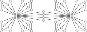
Figure 4. The construction of the graph $R^{\ell,q}(P_{2})$ for $\ell=1$ and $q=2$, where $P_{2}$ is the path with two vertices and one edge.

In the following it is convenient to consider a multivariate version of $Z(G;\mathsf{x},\mathsf{y},\mathsf{z})$ denoted $Z(G;\bar{\mathsf{x}},\bar{\mathsf{y}}.\bar{\mathsf{z}})$. This approach was introduced for the Tutte polynomial by A. Sokal, see [27]. $Z(G;\bar{\mathsf{x}},\bar{\mathsf{y}}.\bar{\mathsf{z}})$ has indeterminates which correspond to every $v\in V(G)$ and every $e\in E(G)$.

Definition 32.

Let $\bar{\mathsf{x}}=\left(\mathsf{x}_{e}:e\in E(G)\right)$, $\bar{\mathsf{y}}=\left(\mathsf{y}_{u}:u\in V(G)\right)$ and $\bar{\mathsf{z}}=\left(\mathsf{z}_{e}:e\in E(G)\right)$ be tuples of distinct indeterminates. Let

$$Z(G;\bar{\mathsf{x}},\bar{\mathsf{y}},\bar{\mathsf{z}})=\sum_{S\subseteq V(G)}\left(\prod_{e\in E_{G}(S)}\mathsf{x}_{e}\right)\left(\prod_{u\in S}\mathsf{y}_{u}\right)\left(\prod_{e\in E_{G}(\bar{S})}\mathsf{z}_{e}\right)\,.$$

We may write $\mathsf{x}_{w,v}$ and $\mathsf{z}_{w,v}$ instead of $\mathsf{x}_{e}$ and $\mathsf{z}_{e}$ for an edge $e=(w,v)$. Clearly, by setting $\mathsf{x}_{e}=\mathsf{x}$ and $\mathsf{z}_{e}=\mathsf{z}$ for every $e\in E(G)$, and $\mathsf{y}_{u}=\mathsf{y}$ for every $u\in V(G)$ we get $Z(G;\bar{\mathsf{x}},\bar{\mathsf{y}},\bar{\mathsf{z}})=Z(G;\mathsf{x},\mathsf{y},\mathsf{z})$.

We furthermore define a variation of $Z(G;\bar{\mathsf{x}},\bar{\mathsf{y}},\bar{\mathsf{z}})$ obtained by restricting the range of the summation variable as follows:

Definition 33.

Given a graph $H$ and $B,C\subseteq V(H)$ with $B$ and $C$ disjoint, let

(11) $$Z(H,B,C;\bar{\mathsf{x}},\bar{\mathsf{y}},\bar{\mathsf{z}})=$$

$$\sum_{A\,:\,B\subseteq A\subseteq V(H)\,,\,A\cap C=\emptyset}\left(\prod_{e\in E_{G}(A)}\mathsf{x}_{e}\right)\left(\prod_{u\in A\setminus B}\mathsf{y}_{u}\right)\left(\prod_{e\in E_{G}(\bar{A})}\mathsf{z}_{e}\right)$$

where the summation is over all $A\subseteq V(H)$, such that $A$ contains $B$ and is disjoint from $C$.

We have $Z(H,\emptyset,\emptyset;\bar{\mathsf{x}},\bar{\mathsf{y}},\bar{\mathsf{z}})=Z(H;\bar{\mathsf{x}},\bar{\mathsf{y}},\bar{\mathsf{z}})$.

4.2. Lemmas, statement of Theorem 2 and its proof

For every edge $e\in E(G)$ between $u$ and $v$, let

$$\omega_{1}(e,S)=Z(N_{\ell}(e)^{+},S\cap\{u,v\},\{u,v\}\setminus S;\bar{\mathsf{x}},\bar{\mathsf{y}},\bar{\mathsf{z}})\,,$$

and for every vertex $w\in V$, let

$$\omega_{2}(w,S)=Z(STh^{\ell}(G_{w}^{q}),S\cap\{w\},\{w\}\setminus S;\bar{\mathsf{x}},\bar{\mathsf{y}},\bar{\mathsf{z}})\,.$$

Let

$$\omega_{1}(S)=\prod_{e\in E(G)}\omega_{1}(e,S)\mbox{\ \ \ and \ \ \ }\omega_{2}(S)=\prod_{w\in V(G)}\omega_{2}(w,S)\,.$$

Let $\omega_{i,\mathrm{\mathrm{triv}}}(S)$ for $i=1,2$ be the polynomials in $\mathsf{x}$, $\mathsf{y}$ and $\mathsf{z}$ obtained from $\omega_{i}(S)$ by setting $\mathsf{x}_{e}=\mathsf{x}$ and $\mathsf{z}_{e}=\mathsf{z}$ for every $e\in E^{\ell,q}$ and $\mathsf{y}_{v}=\mathsf{y}$ for every $v\in V^{\ell,q}_{R}$.

Lemma 34.

$$Z(R^{\ell,q}(G);\mathsf{x}.\mathsf{y}.\mathsf{z})=\sum_{S\subseteq V(G)}\omega_{1,\mathrm{triv}}(S)\cdot\omega_{2,\mathrm{\mathrm{triv}}}(S)\cdot\mathsf{y}^{|S|}\,.$$

Proof.

Each edge of $R^{\ell,q}(G)$ is either contained in some $N_{\ell}(e)^{+}$ for $e\in E(G)$, or in some $STh^{\ell}(G_{w}^{q})$ for $w\in V(G)$. Hence, by the definitions of $Z(R^{\ell,q}(G);\bar{\mathsf{x}},\bar{\mathsf{y}},\bar{\mathsf{z}})$, $\omega_{1}(S)$ and $\omega_{2}(S)$,

$$Z(R^{\ell,q}(G);\bar{\mathsf{x}},\bar{\mathsf{y}},\bar{\mathsf{z}})=\sum_{S\subseteq V(G)}\omega_{1}(S)\cdot\omega_{2}(S)\cdot\prod_{w\in S}\mathsf{y}_{w}$$

holds and the lemma follows. ∎

Lemma 35.

Let $e=(u,w)$ be an edge of $G$. Then

$$\omega_{1,\mathrm{triv}}(e,S)=\begin{cases}(\mathsf{y}+\mathsf{z}^{2})^{4\ell}&|\{u,v\}\cap S|=0\\ (\mathsf{x}\mathsf{y}+\mathsf{z})^{4\ell}&|\{u,v\}\cap S|=1\\ (\mathsf{y}\mathsf{x}^{2}+1)^{4\ell}&|\{u,v\}\cap S|=2\end{cases}$$

Proof.

The value of $\omega_{1}(e,S)$ depends only on whether $u,w\in S$. Consider $A\subseteq V(N_{\ell}(e)^{+})$ which satisfies the summation conditions in Equation (11) for $Z(N_{\ell}(e)^{+},S\cap\{u,w\},\{u,w\}\setminus S;\mathsf{x},\mathsf{y},\mathsf{z})$.

1. If $w\in S$ and $u\notin S$: Exactly one edge $e^{\prime}$ incident to $v_{e,i}$ crosses the cut $[A,\bar{A}]_{N_{\ell}(e)^{+}}$. The other edge $e^{\prime\prime}$ incident to $v_{e,i}$ belongs to $E(A)$ or $E(\bar{A})$, depending on whether $v_{e,i}\in A$. We get:

   $$\omega_{1}(e,S)=\prod_{i=1}^{4\ell}(\mathsf{x}_{v_{e,i},w}\mathsf{y}_{v_{e,i}}+\mathsf{z}_{v_{e,i},u})\,.$$

2. If $w\notin S$ and $u\in S$: this case is similar to the previous case, and we get

   $$\omega_{1}(e,S)=\prod_{i=1}^{4\ell}(\mathsf{x}_{v_{e,i},u}\mathsf{y}_{v_{e,i}}+\mathsf{z}_{v_{e,i},w})\,.$$

3. If $w,u\in S$: For each $v_{e,i}$, either $v_{e,i}\in A$, in which case both edges $(v_{e,i},w)$ and $(v_{e,i},u)$ are in $E(A)$, or $v_{e,i}\notin S$, and both edges $(v_{e,i},w)$ and $(v_{e,i},u)$ cross the cut. We get:

   $$\omega_{1}(e,S)=\prod_{i=1}^{4\ell}(\mathsf{y}_{v_{e,i}}\mathsf{x}_{v_{e,i},u}\mathsf{x}_{v_{e,i},w}+1)\,.$$

4. If $w,u\notin S$: For each $v_{e,i}$, either $v_{e,i}\in S$ and then both edges incident to $v_{e,i}$ cross the cut, or $v_{e,i}\notin S$ and none of the two edges cross the cut. We get:

   $$\omega_{1}(e,S)=\prod_{i=1}^{4\ell}(\mathsf{y}_{v_{e,i}}+\mathsf{z}_{v_{e,i},w}\mathsf{z}_{v_{e,i},u})\,.$$

The lemma follows by setting $\mathsf{x}_{e}=\mathsf{x}$ and $\mathsf{z}_{e}=\mathsf{z}$ for every edge $e$ and $\mathsf{y}_{u}=\mathsf{y}$ for every vertex $u$. ∎

Lemma 36.

Let

$$g_{\ell,q}(\mathsf{x},\mathsf{y},\mathsf{z}) = \mathsf{y}\cdot\left(\mathsf{y}\mathsf{x}^{2}+1\right)^{4\ell}+\left(\mathsf{y}\mathsf{x}+\mathsf{z}\right)^{4\ell}$$

$$h_{\ell,q}(\mathsf{x},\mathsf{y},\mathsf{z}) = \left(\mathsf{y}+\mathsf{z}^{2}\right)^{4\ell}+\mathsf{y}\cdot\left(\mathsf{y}\mathsf{x}+\mathsf{z}\right)^{4\ell}\,.$$

Let $w$ be a vertex of $G$. Then

$$\omega_{2,\mathrm{triv}}(w,S) = \begin{cases}\left(g_{\ell,q}(\mathsf{x},\mathsf{y},\mathsf{z})\right)^{2q}&w\in S\\ \left(h_{\ell,q}(\mathsf{x},\mathsf{y},\mathsf{z})\right)^{2q}&w\notin S\end{cases}$$

Proof.

Consider $A$ which satisfies the summation conditions in Equation (11) for $Z(STh^{\ell}(G_{w}^{q}),S\cap\{w\},\{w\}\setminus S;\bar{\mathsf{x}},\bar{\mathsf{y}},\bar{\mathsf{z}})$.

1. If $w\in S$ (or, equivalently, $c_{w}\in A$): Let $u\in V_{w}^{q}\setminus\left\{c_{w}\right\}$ and $e=\{u,c_{w}\}$. If $u\in A$, then the vertices $u$ and $v_{e,1},\ldots,v_{e,4\ell}$ contribute

   $$\mathsf{y}_{u}\prod_{i=1}^{4\ell}(\mathsf{y}_{v_{e,i}}\mathsf{x}_{v_{e,i},w}\mathsf{x}_{v_{e,i},u}+1)\,.$$

   Otherwise, if $u\notin A$, then the vertices $u$ and $v_{e,1},\ldots,v_{e,4\ell}$ contribute

   $$\prod_{i=1}^{4\ell}(\mathsf{y}_{v_{e,i}}\mathsf{x}_{v_{e,i},w}+\mathsf{z}_{v_{e,i},u})\,.$$

   Hence, $\omega_{2}(w,S)$ equals in this case

   $$\prod_{u\in V^{q}_{w}}\left(\mathsf{y}_{u}\prod_{i=1}^{4\ell}(\mathsf{y}_{v_{e,i}}\mathsf{x}_{v_{e,i},w}\mathsf{x}_{v_{e,i},u}+1)+\prod_{i=1}^{4\ell}(\mathsf{y}_{v_{e,i}}\mathsf{x}_{v_{e,i},w}+\mathsf{z}_{v_{e,i},u})\right)\,.$$

2. If $w\not\in S$ (or, equivalently, $c_{w}\notin A$): Let $u\in V_{w}^{q}\setminus\left\{c_{w}\right\}$ and $e=\{u,c_{w}\}$. If $u\in A$, then the vertices $u$ and $v_{e,1},\ldots,v_{e,4\ell}$ contribute

   $$\mathsf{y}_{u}\prod_{i=1}^{4\ell}(\mathsf{y}_{v_{e,i}}\mathsf{x}_{v_{e,i},u}+\mathsf{z}_{v_{e,i},w})\,.$$

   Otherwise, if $u\notin A$, then the vertices $u$ and $v_{e,1},\ldots,v_{e,4\ell}$ contribute

   $$\prod_{i=1}^{4\ell}(\mathsf{y}_{v_{e,i}}+\mathsf{z}_{v_{e,i},w}\mathsf{z}_{v_{e,i},u})\,.$$

   Hence, $\omega_{2}(w,S)$ equals in this case

   $$\prod_{u\in V^{q}_{w}}\left(\prod_{i=1}^{4\ell}(\mathsf{y}_{v_{e,i}}\mathsf{x}_{v_{e,i},u}+\mathsf{z}_{v_{e,i},w})+\prod_{i=1}^{4\ell}(\mathsf{y}_{v_{e,i}}+\mathsf{z}_{v_{e,i},w}\mathsf{z}_{v_{e,i},u})\right)\,.$$

The lemma follows by setting $\mathsf{x}_{e}=\mathsf{x}$ and $\mathsf{z}_{e}=\mathsf{z}$ for every edge $e$ and $\mathsf{y}_{u}=\mathsf{y}$ for every vertex $u$. ∎

Lemma 37.

If $G$ is $d-$regular, then

$$f_{p,R}(\mathsf{x},\mathsf{y},\mathsf{z},\ell,q)\cdot Z(G;f_{\mathsf{t},R}(\mathsf{x},\mathsf{y},\mathsf{z},\ell),f_{\mathsf{y},R}(\mathsf{x},\mathsf{y},\mathsf{z},\ell,q))=Z(R^{\ell,q}(G);\mathsf{x},\mathsf{y},\mathsf{z})$$

where

$$f_{p,R}(\mathsf{x},\mathsf{y},\mathsf{z},\ell,q) = \left(h_{\ell,q}(\mathsf{x},\mathsf{y},\mathsf{z})\right)^{2qn_{G}}(\mathsf{y}+\mathsf{z}^{2})^{2\ell dn_{G}}\,,$$

$$f_{\mathsf{t},R}(\mathsf{x},\mathsf{y},\mathsf{z},\ell) = \left(\frac{(\mathsf{y}\mathsf{x}+\mathsf{z})^{2}}{(\mathsf{y}\mathsf{x}^{2}+1)(\mathsf{y}+\mathsf{z}^{2})}\right)^{2\ell}\,,$$

$$f_{\mathsf{y},R}(\mathsf{x},\mathsf{y},\mathsf{z},\ell,q) = \mathsf{y}\cdot\left(\frac{\mathsf{y}\mathsf{x}^{2}+1}{\mathsf{y}+\mathsf{z}^{2}}\right)^{2\ell d}\left(\frac{g_{\ell,q}(\mathsf{x},\mathsf{y},\mathsf{z})}{h_{\ell,q}(\mathsf{x},\mathsf{y},\mathsf{z})}\right)^{2q}\,.$$

Proof.

We want to rewrite $Z(R^{\ell,q}(G);\bar{\mathsf{x}},\bar{\mathsf{y}},\bar{\mathsf{z}})$ as a sum over subsets $S$ of vertices of $G$. Using Lemma 34, in order to compute $Z(R^{\ell,q}(G);\mathsf{x},\mathsf{y},\mathsf{z})$ we first need to find $\omega_{1,\mathrm{triv}}(S)$ and $\omega_{2,\mathrm{triv}}(S)$. Using Lemma 36, $\omega_{2,\mathrm{triv}}(S)$ is given by

$$\omega_{2,\mathrm{triv}}(S)=\left(g_{\ell,q}(\mathsf{x},\mathsf{y},\mathsf{z})\right)^{2q|S|}\cdot\left(h_{\ell,q}(\mathsf{x},\mathsf{y},\mathsf{z})\right)^{2qn_{G}-2q|S|}\,.$$

In order to compute $\omega_{1,\mathrm{triv}}(S)$, consider $S\subseteq V(G)$. Since $G$ is $d$-regular, the number of edges contained in $S$ is $\frac{1}{2}(d\cdot|S|-|[S,\bar{S}]_{G}|)$, and the number of edges contained in $\bar{S}$ is $\frac{1}{2}(dn_{G}-d\cdot|S|-|[S,\bar{S}]_{G}|)$. Hence, by Lemma 35, $\omega_{1,\mathrm{triv}}(S)$ is given by

$$\omega_{1,\mathrm{triv}}(S)=(\mathsf{x}\mathsf{y}+\mathsf{z})^{4\ell|[S,\bar{S}]_{G}|}(\mathsf{y}\mathsf{x}^{2}+1)^{4\ell\cdot\frac{d\cdot|S|-|[S,\bar{S}]_{G}|}{2}}(\mathsf{y}+\mathsf{z}^{2})^{4\ell\cdot\frac{dn_{G}-d\cdot|S|-|[S,\bar{S}]_{G}|}{2}}\,.$$

Using Lemma 34,

$$Z(R^{\ell,q}(G);\mathsf{x},\mathsf{y},\mathsf{z})=\sum_{S\subseteq V(G)}\omega_{1,\mathrm{triv}}(S)\cdot\omega_{2,\mathrm{triv}}(S)\cdot\mathsf{y}^{|S|}$$

which is equal to $(\mathsf{y}+\mathsf{z}^{2})^{4\ell\cdot\frac{dn_{G}}{2}}$ times

(12) $$\sum_{S\subseteq V(G)}\left(\frac{(\mathsf{y}\mathsf{x}+\mathsf{z})^{2}}{(\mathsf{y}\mathsf{x}^{2}+1)(\mathsf{y}+\mathsf{z}^{2})}\right)^{2\ell|[S,\bar{S}]_{G}|}\left(\mathsf{y}\cdot\left(\frac{\mathsf{y}\mathsf{x}^{2}+1}{\mathsf{y}+\mathsf{z}^{2}}\right)^{2\ell d}\right)^{|S|}\cdot\omega_{2,\mathrm{triv}}(S)\,.$$

Plugging the expression for $\omega_{2,\mathrm{triv}}(S)$ in Equation (12), we get that $Z(R^{\ell,q}(G);\mathsf{x},\mathsf{y},\mathsf{z})$ equals $f_{p,R}(\mathsf{x},\mathsf{y},\mathsf{z},\ell,q)$ times

$$\sum_{S\subseteq V(G)}\left(\frac{(\mathsf{y}\mathsf{x}+\mathsf{z})^{2}}{(\mathsf{y}\mathsf{x}^{2}+1)(\mathsf{y}+\mathsf{z}^{2})}\right)^{2\ell|[S,\bar{S}]_{G}|}\left(\mathsf{y}\cdot\left(\frac{\mathsf{y}\mathsf{x}^{2}+1}{\mathsf{y}+\mathsf{z}^{2}}\right)^{2\ell d}\left(\frac{g_{\ell,q}(\mathsf{x},\mathsf{y},\mathsf{z})}{h_{\ell,q}(\mathsf{x},\mathsf{y},\mathsf{z})}\right)^{2q}\right)^{|S|}$$

and the lemma follows. ∎

Lemma 38.

Let $e\in\mathbb{Q}\backslash\left\{-1,0,1\right\}$ and let $a,b,c>0$ and $b\not=c$. Then there is $c_{1}\in\mathbb{N}$ for which the sequence

(13) $$h(\ell)=\frac{e\cdot b^{\ell}+a^{\ell}}{c^{\ell}+e\cdot a^{\ell}}$$

is strictly monotone increasing or decreasing for $\ell\geq c_{1}$.

Proof.

$h(\ell)$ can be rewritten as

$$h(\ell) = \frac{e\cdot{\tilde{b}}^{\ell}+1}{{\tilde{c}}^{\ell}+e}$$

by dividing both the numerator and the denominator of the right-hand side of Equation (13) by $a^{\ell}$ and setting ${\tilde{b}}=\frac{b}{a}$ and ${\tilde{c}}=\frac{c}{a}$. We have ${\tilde{b}}\not={\tilde{c}}$ and ${\tilde{b}},{\tilde{c}}>0$.

Let $h(x)=\frac{e\cdot{\tilde{b}}^{x}+1}{{\tilde{c}}^{x}+e}$. The derivative of $h(x)$ is given by

(14) $$h^{\prime}(x) = \frac{e\ln{\tilde{b}}\cdot{\tilde{b}}^{x}\left({\tilde{c}}^{x}+e\right)-\ln{\tilde{c}}\cdot{\tilde{c}}^{x}\left(e\cdot{\tilde{b}}^{x}+1\right)}{({\tilde{c}}^{x}+e)^{2}}$$

$$= \frac{e^{2}\ln{\tilde{b}}\cdot{\tilde{b}}^{x}-\ln{\tilde{c}}\cdot{\tilde{c}}^{x}+e(\ln{\tilde{b}}-\ln{\tilde{c}}){\tilde{b}}^{x}{\tilde{c}}^{x}}{({\tilde{c}}^{x}+e)^{2}}$$

The denominator of $h^{\prime}(x)$ is non-zero for large enough $x$. Therefore, there exists $x_{0}$ such that $h^{\prime}(x)$ is continuous on $[x_{0},\infty)$, so it is enough to show that $h^{\prime}(x)\not=0$ for all large enough $x$ to get the desired result.

If ${\tilde{b}}=1$ then $({\tilde{c}}^{x}+e)^{2}h^{\prime}(x)=-(1+e)\ln{\tilde{c}}\cdot{\tilde{c}}^{x}$, and if ${\tilde{c}}=1$ then $({\tilde{c}}^{x}+e)^{2}h^{\prime}(x)=(e^{2}+e)\ln{\tilde{b}}\cdot{\tilde{b}}^{x}$. In both cases $h^{\prime}(x)$ is non-zero, using that ${\tilde{b}}\not={\tilde{c}}$ and ${\tilde{b}},{\tilde{c}}>0$.

Otherwise, ${\tilde{b}}$, ${\tilde{c}}$ and ${\tilde{b}}{\tilde{c}}$ are distinct. Let $A_{1}=\{{\tilde{b}}^{x},{\tilde{c}}^{x},{\tilde{b}}^{x}{\tilde{c}}^{x}\}$. Let $A_{2}$ be the subset of $A_{1}$ which contains the functions of $A_{1}$ which have non-zero coefficients in Equation (14). Note ${\tilde{b}}^{x}{\tilde{c}}^{x}$ belongs of $A_{2}$. There is a function in $A_{2}$ which dominates the other functions of $A_{2}$. This implies that $h^{\prime}(x)$ is non-zero for large enough values of $x$. ∎

Theorem 2 is now given precisely and proved:

Theorem 39.

For all $(\gamma,\delta,\varepsilon)\in\mathbb{Q}^{3}$ such that

1. $\delta\not=\{-1,0,1\}$,

2. $\delta+\varepsilon^{2}\notin\{-1,0,1\}$,

3. $\delta+\varepsilon^{2}\not=\pm(\delta\gamma^{2}+1)$,

4. $\delta\gamma^{2}+1\not=0$,

5. $\gamma\delta+\varepsilon\not=0$, and

6. $(\gamma\delta+\varepsilon)^{4}\not=\left(\delta\gamma^{2}+1\right)^{2}\left(\delta+\varepsilon^{2}\right)^{2}$.

$Z(-;\gamma,\delta,\varepsilon)$ is $\mathrm{\mathbf{\#P}}$-hard on simple bipartite planar graphs.

Proof.

We will show that, on $3-$regular bipartite planar graphs $G$, the polynomial $Z(G;\mathsf{t},\mathsf{y})$ is polynomial-time computable using oracle calls to $Z(-;\gamma,\delta,\varepsilon)$. The oracle is only queried with input of simple bipartite planar graphs. Using Proposition 8, computing $Z(G;\mathsf{t},\mathsf{y})$ is $\mathrm{\mathbf{\#P}}$-hard on $3$-regular bipartite planar graphs.

Using (i) and (ii) it can be verified that there exists $c_{0}\in\mathbb{N}^{+}$ such that for all $\ell\geq c_{0}$ and $q\in\mathbb{N}^{+}$, $f_{p,R}(\gamma,\delta,\varepsilon,2\ell,q)\not=0$. We can use Lemma 37 to manufacture, in polynomial-time, evaluations of $Z(G;\mathsf{t},\mathsf{y})$ that will be used to interpolate $Z(G;\mathsf{t},\mathsf{y})$.

Let $\ell\geq c_{0}$ and let

$$E_{\mathsf{y},1}=\frac{\delta\gamma^{2}+1}{\delta+\varepsilon^{2}}\mbox{\ \ \ and \ \ \ }E_{\mathsf{y},2,\ell}=\frac{\delta(\delta\gamma^{2}+1)^{4\ell}+(\gamma\delta+\varepsilon)^{4\ell}}{(\delta+\varepsilon^{2})^{4\ell}+\delta(\gamma\delta+\varepsilon)^{4\ell}}\,.$$

We have that $f_{\mathsf{y},R}(\gamma,\delta,\varepsilon,\ell,q)=\delta\left(E_{\mathsf{y},1}\right)^{2d\ell}\left(E_{\mathsf{y},2,\ell}\right)^{2q}$. Using (iv) we have $E_{\mathsf{y},1}\not=0$.

Look at $E_{\mathsf{y},2,\ell}$ as a function of $\ell$. Using (i), (ii), (iii) and (iv) and Lemma 38 with $a=(\gamma\delta+\varepsilon)^{4}$, $b=(\delta\gamma^{2}+1)^{4}$, $c=(\delta+\varepsilon^{2})^{4}$ and $e=\delta$, there exists $c_{1}$ such that $E_{\mathsf{y},2,\ell}$ is strictly monotone increasing or decreasing. Hence, there exists $c_{2}\geq c_{1}$ such that, for every $\ell\geq c_{2}$, $E_{\mathsf{y},2,\ell}\notin\{-1,0,1\}$. Moreover, $c_{2}=c_{2}(\gamma,\delta,\varepsilon)$ is a function of $\gamma$, $\delta$ and $\varepsilon$.

We get that for $q_{1}\not=q_{2}\in[n_{G}+1]$ and $\ell>c_{2}$, $\left(E_{\mathsf{y},2,\ell}\right)^{2q_{1}}\not=\left(E_{\mathsf{y},2,\ell}\right)^{2q_{2}}$. Since $\delta\left(E_{y,1}\right)^{2d\ell}$ is not equal to $0$ and does not depend on $q$, we get that for $q_{1}\not=q_{2}\in[n_{G}+1]$, $f_{\mathsf{y},R}(\gamma,\delta,\varepsilon,\ell,q_{1})\not=f_{\mathsf{y},R}(\gamma,\delta,\varepsilon,\ell,q_{2})$.

For every $\ell\in[m_{G}+c_{2}+1]\setminus[c_{2}]$, we can interpolate in polynomial-time the univariate polynomial $Z(G;f_{\mathsf{t},R}(\gamma,\delta,\varepsilon,\ell),\mathsf{y})$. Then, we can use the polynomial $Z(G;f_{\mathsf{t},R}(\gamma,\delta,\varepsilon,\ell),\mathsf{y})$ to compute $Z(G;f_{\mathsf{t},R}(\gamma,\delta,\varepsilon,\ell),j)$ for every $\ell\in[m_{G}+c_{2}+1]\setminus[c_{2}]$ and every $j\in[n_{G}+1]$. Let

$$E_{\mathsf{t}}=\left(\frac{(\gamma\delta+\varepsilon)^{2}}{(\delta\gamma^{2}+1)(\delta+\varepsilon^{2})}\right)^{2}$$

and it holds that $f_{\mathsf{t},R}(\gamma,\delta,\varepsilon,\ell,q)=\left(E_{\mathsf{t}}\right)^{\ell}$. Clearly, $E_{\mathsf{t}}\not=-1$ and, by (v) and (vi), $E_{\mathsf{t}}\notin\{0,1\}$. Hence, for every $\ell_{1}\not=\ell_{2}\in\mathbb{N}^{+}$ we have $f_{\mathsf{t},R}(\gamma,\delta,\varepsilon,\ell_{1})\not=f_{\mathsf{t},R}(\gamma,\delta,\varepsilon,\ell_{2})$. Therefore, we can compute the value of the bivariate polynomial $Z(G;\mathsf{t},\mathsf{y})$ on a grid of points of size $(m_{G}+1)\times(n_{G}+1)$ in polynomial-time using the oracle, and use them to interpolate $Z(G;\mathsf{t},\mathsf{y})$.
  ∎

5. Computation on Graphs of Bounded Clique-width

In this section we prove Theorem 3. Let $G$ be a graph and let $cw(G)$ be its clique-width. As discussed in Section 2.3, a $k$-expression $t(G)$ for $G$ with $k\leq 2^{3cw(G)+2}-1$ can be computed in $\mathrm{\mathbf{FPT}}$-time. Let $\bar{c}=(c_{v}:v\in V(G))$ be the labels from $[k]$ associated with the vertices of $G$ by $t(G)$. We will show how to compute a multivariate polynomial $Z_{\mathrm{labeled}}(G,\bar{c};\bar{\mathsf{x}},\bar{\mathsf{y}},\bar{\mathsf{z}})$ with indeterminate set

$$\left\{\mathsf{x}_{\{i,j\}},\mathsf{y}_{i},\mathsf{z}_{\{i,j\}}\mid i,j\in[k]\right\}$$

to be defined below. Note it is not the same multivariate polynomial as in Section 4. For simplicity of notation we write e.g. $\mathsf{x}_{i,j}$ or $\mathsf{x}_{j,i}$ for $\mathsf{x}_{\{i,j\}}$. The multivariate polynomial $Z_{\mathrm{labeled}}(G,\bar{c};\bar{\mathsf{x}},\bar{\mathsf{y}},\bar{\mathsf{z}})$ is defined as

(15) $$\sum_{S\subseteq V(G)}\,\left(\prod_{v\in S}\mathsf{y}_{c_{v}}\right)\left(\prod_{(u,v)\in E_{G}(S)}\mathsf{x}_{c_{u},c_{v}}\right)\left(\prod_{(u,v)\in E_{G}(\bar{S})}\mathsf{z}_{c_{u},c_{v}}\right)\,.$$

The left-most product in Equation (15) is over all vertices $v$ in $S$. The two other products are over all edges in $E_{G}(S)$ and $E_{G}(\bar{S})$ respectively. It is not hard to see that $Z(G;\mathsf{x},\mathsf{y},\mathsf{z})$ is obtained from $Z_{\mathrm{labeled}}(G,\bar{c};\bar{\mathsf{x}},\bar{\mathsf{y}},\bar{\mathsf{z}})$ by substituting all the indeterminates $\mathsf{x}_{i,j}$, $\mathsf{y}_{i}$ and $\mathsf{z}_{i,j}$ by three indeterminates, $\mathsf{x}$, $\mathsf{y}$ and $\mathsf{z}$, respectively.

Given tuples of natural numbers $\bar{\mathpzc{a}}=(\mathpzc{a}_{i}\,:\,i\in[k])$, $\bar{\mathpzc{b}}=(\mathpzc{b}_{i,j}\,:\,i,j\in[k])$ and $\bar{\mathpzc{c}}=(\mathpzc{c}_{i,j}\,:\,i,j\in[k])$, we denote by $t_{\bar{\mathpzc{a}},\bar{\mathpzc{b}},\bar{\mathpzc{c}}}(G)$ the coefficient of the monomial

$$\prod_{i\in[k]}\mathsf{y}_{i}^{\mathpzc{a}_{i}}\prod_{i,j\in k}\mathsf{x}_{i,j}^{\mathpzc{b}_{i,j}}\mathsf{z}_{i,j}^{\mathpzc{c}_{i,j}}$$

in $Z_{\mathrm{labeled}}(G;\bar{\mathsf{x}},\bar{\mathsf{y}},\bar{\mathsf{z}})$. We call a triple $(\bar{\mathpzc{a}},\bar{\mathpzc{b}},\bar{\mathpzc{c}})$ valid if $\mathpzc{a}_{1}+\ldots+\mathpzc{a}_{k}\leq n_{G}$ and, for all $i,j\in[k]$, $\mathpzc{b}_{i,j},\mathpzc{c}_{i,j}\leq m_{G}$. If $(\bar{\mathpzc{a}},\bar{\mathpzc{b}},\bar{\mathpzc{c}})$ is not valid, then $t_{\bar{\mathpzc{a}},\bar{\mathpzc{b}},\bar{\mathpzc{c}}}(G)=0$. Therefore, to determine the polynomial $Z_{\mathrm{labeled}}(G;\bar{\mathsf{x}},\bar{\mathsf{y}},\bar{\mathsf{z}})$ we need only to find $t_{\bar{\mathpzc{a}},\bar{\mathpzc{b}},\bar{\mathpzc{c}}}(G)$ for all valid triples $(\bar{\mathpzc{a}},\bar{\mathpzc{b}},\bar{\mathpzc{c}})$.

The $t_{\bar{\mathpzc{a}},\bar{\mathpzc{b}},\bar{\mathpzc{c}}}(G)$ form an $\left(k+2k^{2}\right)$-dimensional array with $\left(\max\left\{n_{G},m_{G}\right\}\right)^{k+2k^{2}}$ integer entries. Each entry in this table can be bounded from above by $2^{n_{G}}$ and thus can be written in polynomial space, so the size of the table is of the form $n_{G}{}^{p_{1}(cw(G))}$, where $p_{1}$ is a function of $cw(G)$ which does not depend on $n_{G}$.

We compute $Z_{\mathrm{labeled}}(G,\bar{c};\bar{\mathsf{x}},\bar{\mathsf{y}},\bar{\mathsf{z}})$ of $G$ by dynamic programming on the structure of the $k$-expression of $G$.

Algorithm 40.

1. If $(G,i)$ is a singleton of any color $i$, $Z_{\mathrm{labeled}}(G,\bar{c};\bar{\mathsf{x}},\bar{\mathsf{y}},\bar{\mathsf{z}})=1+\mathsf{y}_{i}$.

2. If $(G,\bar{c})$ is the disjoint union of $(H,\bar{c}_{H_{1}})$ and $(H_{2},\bar{c}_{H_{2}})$, then

   $$Z_{\mathrm{labeled}}(G,\bar{c};\bar{\mathsf{x}},\bar{\mathsf{y}},\bar{\mathsf{z}})=Z_{\mathrm{labeled}}(H_{1},\bar{c}_{H_{1}};\bar{\mathsf{x}},\bar{\mathsf{y}},\bar{z})\cdot Z_{\mathrm{labeled}}(H_{2},\bar{c}_{H_{2}};\bar{\mathsf{x}},\bar{\mathsf{y}},\bar{z})\,.$$

3. If $(G,\bar{c})=\eta_{p,r}(H,\bar{c}_{H})$: let $\mathpzc{d}_{r}$ and $\mathpzc{d}_{p}$ be the number of vertices of colors $r$ and $p$ in $H$, respectively.

   1. For every valid $(\bar{\mathpzc{a}},\bar{\mathpzc{b}},\bar{\mathpzc{c}})$, if

      (16) $$\mathpzc{b}_{p,r}=\begin{cases}\mathpzc{a}_{p}\cdot\mathpzc{a}_{r}&p\not=r\\ \binom{\mathpzc{a}_{p}}{2}&p=r\end{cases}\mbox{\ \ \ and \ \ \ }\mathpzc{c}_{p,r}=\begin{cases}(\mathpzc{d}_{p}-\mathpzc{a}_{p})\cdot(\mathpzc{d}_{r}-\mathpzc{a}_{r})&p\not=r\\ \binom{\mathpzc{d}_{p}-\mathpzc{a}_{p}}{2}&p=r\end{cases}$$

      set

      $$t_{\bar{\mathpzc{a}},\bar{\mathpzc{b}},\bar{\mathpzc{c}}}(G)=\sum_{\bar{\mathpzc{b}^{\prime}},\bar{\mathpzc{c}^{\prime}}}t_{\bar{\mathpzc{a}},\bar{\mathpzc{b}^{\prime}},\bar{\mathpzc{c}^{\prime}}}(H)$$

      where the summation is over all valid tuples $\bar{\mathpzc{b}}^{\prime}=(\mathpzc{b}_{i,j}^{\prime}\,:\,i,j\in[k])$ and $\bar{\mathpzc{c}}^{\prime}=(\mathpzc{c}_{i,j}^{\prime}\,:\,i,j\in[k])$ such that $\mathpzc{b}_{i,j}^{\prime}=\mathpzc{b}_{i,j}$ and $\mathpzc{c}_{i,j}^{\prime}=\mathpzc{c}_{i,j}$ if $\{i,j\}\not=\{p,r\}$.

   2. For every valid $(\bar{\mathpzc{a}},\bar{\mathpzc{b}},\bar{\mathpzc{c}})$, if Equation (16) does not hold, set $t_{\bar{\mathpzc{a}},\bar{\mathpzc{b}},\bar{\mathpzc{c}}}(G)=0$.

4. If $(G,\bar{c})=\rho_{p\to r}(H,\bar{c}_{H})$:

   1. For every valid $(\bar{\mathpzc{a}},\bar{\mathpzc{b}},\bar{\mathpzc{c}})$ if $\mathpzc{a}_{p}=0$, set

      $$t_{\bar{\mathpzc{a}},\bar{\mathpzc{b}},\bar{\mathpzc{c}}}(G)=\sum_{\bar{\mathpzc{a}}^{\prime},\bar{\mathpzc{b}}^{\prime},\bar{\mathpzc{c}}^{\prime}}t_{\bar{\mathpzc{a}}^{\prime},\bar{\mathpzc{b}}^{\prime},\bar{\mathpzc{c}}^{\prime}}(H)$$

      where the summation is over all valid tuples $\bar{\mathpzc{a}}^{\prime}=(\mathpzc{a}_{i}^{\prime}\,:\,i\in[k])$, $\bar{\mathpzc{b}}^{\prime}=(\mathpzc{b}_{i,j}^{\prime}\,:\,i,j\in[k])$ and $\bar{\mathpzc{c}}^{\prime}=(\mathpzc{c}_{i,j}^{\prime}\,:\,i,j\in[k])$ such that

      • $\mathpzc{a}_{r}=\mathpzc{a}_{p}^{\prime}+\mathpzc{a}_{r}^{\prime}$,

      • $\mathpzc{a}_{i}=\mathpzc{a}_{i}^{\prime}$ for all $i\notin\{p,r\}$,

      • for all $j\in[k]\setminus\{p\}$,

        $$\mathpzc{b}_{j,r}=\begin{cases}\mathpzc{b}_{j,p}^{\prime}+\mathpzc{b}_{j,r}^{\prime}&\mbox{ if }j\not=r\\ \mathpzc{b}_{r,r}^{\prime}+\mathpzc{b}_{p,r}^{\prime}+\mathpzc{b}_{p,p}^{\prime}&\mbox{ if }j=r\end{cases}\mbox{\ \ \ and \ \ \ }\mathpzc{c}_{j,r}=\begin{cases}\mathpzc{c}_{j,p}^{\prime}+\mathpzc{c}_{j,r}^{\prime}&\mbox{ if }j\not=r\\ \mathpzc{c}_{r,r}^{\prime}+\mathpzc{c}_{p,r}^{\prime}+\mathpzc{c}_{p,p}^{\prime}&\mbox{ if }j=r\end{cases}$$

        and

      • for all $i,j\in[k]\setminus\{p,r\}$, $\mathpzc{b}_{i,j}=\mathpzc{b}_{i,j}^{\prime}$ and $\mathpzc{c}_{i,j}=\mathpzc{c}_{i,j}^{\prime}$.

   2. For every For every valid $(\bar{\mathpzc{a}},\bar{\mathpzc{b}},\bar{\mathpzc{c}})$ if $\mathpzc{a}_{p}\not=0$, set $t_{\bar{\mathpzc{a}},\bar{\mathpzc{b}},\bar{\mathpzc{c}}}(G)=0$.

Correctness:

1. By direct computation.

2. Proved in [2] for $Z(G;\mathsf{t},\mathsf{y})$. The trivariate case is similar.

3. $G=\eta_{p,r}(H)$: Let $S$ be a subset of vertices of $V(G)=V(H)$ with $\mathpzc{a}_{p}$ and $\mathpzc{a}_{r}$ vertices of colors $p$ and $r$ respectively. After adding all possible edges between vertices of color $p$ and of color $r$ in $S$, the number of edges between such vertices in $E_{G}(S)$ is $\mathpzc{a}_{p}\cdot\mathpzc{a}_{r}$ if $r\not=p$ and $\binom{\mathpzc{a}_{p}}{2}$ if $p=r$. Similarly, the number of edges between vertices colored $p$ and $r$ in $E_{G}(\bar{S})$ is $(\mathpzc{d}_{p}-\mathpzc{a}_{p})\cdot(\mathpzc{d}_{r}-\mathpzc{a}_{r})$ if $r\not=p$ and $\binom{\mathpzc{d}_{p}-\mathpzc{a}_{p}}{2}$ if $p=r$.

4. $G=\rho_{p\to r}(H)$: Let $S$ be a subset of vertices of $V(G)=V(H)$. After recoloring every vertex of color $p$ in $S$ to color $r$, we have $\mathpzc{a}_{p}=0$. Every edge between a vertex colored $p$ to any other vertex lies after the recoloring between a vertex colored $r$ and another vertex. There is one special case, which is the edges that lie between vertices colored $r$ after the recoloring. Before the recoloring these edges were incident to vertices colored any combination of $p$ and $r$.

Running Time:

The size of the $(2^{3cw(G)+2}-1)$-expression is bounded by $n^{c}\cdot f_{1}(k)$ for some constant $c$, which does not depend on $cw(G)$, and for some function $f_{1}$ of $cw(G)$. Now we look at the possible operations performed by Algorithm 40:

1. The time does not depend on $n$ since $G$ is of size $O(1)$.

2. The time can be bounded by the size of the table $t_{\bar{\mathpzc{a}},\bar{\mathpzc{b}},\bar{\mathpzc{c}}}$ to the power of $3$, i.e. $n^{3p_{1}(cw(G))}$.

3. For $\mu_{p,r}$, the algorithm loops over all the values in the table $t_{\bar{\mathpzc{a}},\bar{\mathpzc{b}},\bar{\mathpzc{c}}}$, and for each entry possibly compute a sum over at most $m_{G}$ elements. Then, the algorithm loops over all the values again and performs $O(1)$ operations.

4. For $\rho_{p\to r}$, the algorithm loops over all the values in the table $t_{\bar{\mathpzc{a}},\bar{\mathpzc{b}},\bar{\mathpzc{c}}}$, and for each entry possibly compute a sum over elements of the table $t_{\bar{\mathpzc{a}},\bar{\mathpzc{b}},\bar{\mathpzc{c}}}$. Then, the algorithm loops over all the values again and performs $O(1)$ operations.

Hence, Algorithm 40 runs in time $O\left(n_{G}^{f(cw(G))}\right)$ for some function $f$.

6. Conclusion and Open Problems

Applying the reductions used in the proof of Theorem 1 to planar graphs gives again planar graphs. Combining Theorem 1 and its proof with Lemma 37, a hardness result for the trivariate Ising polynomial on planar graphs analogous to Theorem 2 follows. However, both Theorem 2 and the analog for planar graphs are not dichotomy theorems since each of them leaves an exceptional set of low dimension unresolved. Theorem 2 serves mainly to suggest the existence of a dichotomy theorem for $Z(G;\mathsf{x},\mathsf{y},\mathsf{z})$ on bipartite planar graphs.

Another open problem which arises from the paper is whether $Z(G;\mathsf{x},\mathsf{y},\mathsf{z})$ requires exponential time to compute in general under $\mathrm{\mathbf{\#ETH}}$. One approach to the latter problem would be to prove that, say, the permanent or the number of maximum cuts require exponential time under $\mathrm{\mathbf{\#ETH}}$ even when restricted to regular graphs.

References

- [1]
- [2] D. Andrén and K. Markström. The bivariate Ising polynomial of a graph. Discrete Applied Mathematics, 157(11):2515–2524, 2009.
- [3] A. Andrzejak. An algorithm for the Tutte polynomials of graphs of bounded treewidth. DMATH: Discrete Mathematics, 190, 1998.
- [4] A.A. Bulatov and M. Grohe. The complexity of partition functions. Theoretical Computer Science, 348(2–3):148–186, 2005.
- [5] J. Cai, X. Chen, and P. Lu. Graph homomorphisms with complex values: A dichotomy theorem. In ICALP (1), volume 6198 of Lecture Notes in Computer Science, pages 275–286. Springer, 2010.
- [6] B. Courcelle and S. Olariu. Upper bounds to the clique width of graphs. Discrete Applied Mathematics, 101(1-3):77–114, 2000.
- [7] H. Dell, T. Husfeldt, and M. Wahlen. Exponential time complexity of the permanent and the Tutte polynomial. In S. Abramsky, C. Gavoille, C. Kirchner, F. Meyer auf der Heide, and P.G. Spirakis, editors, ICALP (1), volume 6198 of LNCS, pages 426–437. Springer, 2010.
- [8] M. Dyer and C. Greenhill. The complexity of counting graph homomorphisms. Random Structures & Algorithms, 17(3–4):260–289, 2000.
- [9] D. L. Vertigan F. Jaeger and D. J. A. Welsh. On the computational complexity of the Jones and Tutte polynomials. Mathematical Proceedings of the Cambridge Philosophical Society, 108:35–53, 1990.
- [10] M.E. Fisher. On the dimer solution of planar ising models. J. Math. Phys., 7:1776–1781, 1966.
- [11] P. Flajolet and R. Sedgewick. Analytic Combinatorics. Cambridge University Press, 2009.
- [12] F.V. Fomin, P.A. Golovach, D. Lokshtanov, and S. Saurabh. Algorithmic lower bounds for problems parameterized with clique-width. In M. Charikar, editor, SODA, pages 493–502. SIAM, 2010.
- [13] O. Giménez, P. Hlinený, and M. Noy. Computing the Tutte polynomial on graphs of bounded clique-width. SIAM J. Discrete Math, 20(4):932–946, 2006.
- [14] L.A. Goldberg, M. Grohe, M. Jerrum, and M. Thurley. A complexity dichotomy for partition functions with mixed signs. SIAM Journal on Computing, 39(7):3336–3402, 2010.
- [15] L.A. Goldberg, M. Jerrum, and M. Paterson. The computational complexity of two-state spin systems. Random Struct. Algorithms, 23(2):133–154, 2003.
- [16] R.L. Graham, D. E. Knuth, and O. Patashnik. Concrete Mathematics. Addison-Wesley, second edition, 1994.
- [17] R. Impagliazzo and R. Paturi. Complexity of k-SAT. In Proceedings of the 14th Annual IEEE Conference on Computational Complexity (CCC-99), pages 237–240, Los Alamitos, May 4–6 1999. IEEE Computer Society.
- [18] M. Jerrum and A. Sinclair. Polynomial-time approximation algorithms for the Ising model. SICOMP: SIAM Journal on Computing, 22, 1993.
- [19] P.W. Kasteleyn. Graph theory and crystal physics. Graph Theory and Theoretical Physics, pages 43–110, 1967.
- [20] J.A. Makowsky. Algorithmic uses of the Feferman-Vaught theorem. Annals of Pure and Applied Logic, 126(1-3):159–213, 2004.
- [21] J.A. Makowsky, U. Rotics, I. Averbouch, and Benny Godlin. Computing graph polynomials on graphs of bounded clique-width. In F.V. Fomin, editor, WG, volume 4271 of Lecture Notes in Computer Science, pages 191–204. Springer, 2006.
- [22] S.D. Noble. Evaluating the Tutte polynomial for graphs of bounded tree-width. In Combinatorics, Probability and Computing, Cambridge University Press, volume 7. 1998.
- [23] S.D. Noble. Evaluating a weighted graph polynomial for graphs of bounded tree-width. Electron, J. Combin., 16(1), 2009.
- [24] S. Oum. Approximating rank-width and clique-width quickly. In D. Kratsch, editor, WG, volume 3787 of Lecture Notes in Computer Science, pages 49–58. Springer, 2005.
- [25] S. Oum and P. Seymour. Approximating clique-width and branch-width. JCTB: Journal of Combinatorial Theory, Series B, 96, 2006.
- [26] A. Sinclair, P. Srivastava, and M. Thurley. Approximation algorithms for two-state anti-ferromagnetic spin systems on bounded degree graphs, July 13 2011.
- [27] A.D. Sokal. The multivariate Tutte polynomial (alias Potts model) for graphs and matroids. In B.S. Webb, editor, Surveys in Combinatorics, volume 327 of London Mathematical Society Lecture Note Series, pages 173–226. Cambridge University Press, 2005.
- [28] M. Thurley. The Complexity of Partition Functions. PhD thesis, Humboldt Universität zu Berlin.
- [29] B.L. van der Waerden. Die lange reichweite der regelmässigen atomanordnung in mischkristallen. Zeitschrift für Physik, 118:573–479, 1941.
- [30] D. Vertigan. The computational complexity of tutte invariants for planar graphs. SICOMP: SIAM Journal on Computing, 35, 2006.
- [31] D. Vertigan and D.J.A. Welsh. The computational complexity of the Tutte plane: the bipartite case. Combinatorics, Probability & Computing, 1:181–187, 1992.
- [32] M. Xia, P. Zhang, and W. Zhao. Computational complexity of counting problems on 3-regular planar graphs. Theoretical Computer Science, 384(1):111–125, 2007.
- [33] J. Zhang, H. Liang, and F. Bai. Approximating partition functions of the two-state spin system. Inf. Process. Lett., 111(14):702–710, 2011.