Shapes of Tight Composite Knots

Abstract

We present new computations of tight shapes obtained using the constrained gradient descent code ridgerunner for 544 composite knots with 12 and fewer crossings, expanding our dataset to 943 knots and links. We use the new data set to analyze two outstanding conjectures about tight knots, namely that the ropelengths of composite knots are at least $4\pi-4$ less than the sums of the prime factors and that the writhes of composite knots are the sums of the writhes of the prime factors.

Keywords: ropelength, tight knots, ideal knots, constrained gradient descent, sparse non-negative least squares problem (snnls), knot-tightening

1 Introduction

When people are given a piece of rope, they almost instinctively tie it into a knot and pull it tight. But what, exactly, is the structure of that tight knot? The last decade has seen great progress in analyzing tight configurations. Researchers have focused on mathematical knots, that is closed loops forming different topological knot types, with the rope modeled as a non self-intersecting tube about a smooth (usually $C^{2}$ or $C^{1,1}$) space curve. One can then define the ropelength of the curve to be the quotient of its length and the maximal radius (or thickness) of a non self-intersecting tube about the curve. Alternately, the ropelength is the minimal centerline length of a unit radius tube without self-intersections forming the given knot type.

Configurations that minimize the ropelength within a given knot type are called tight or ideal. These configurations have been used to predict the relative speed of DNA knots under gel electrophoresis [1], the pitch of double helical DNA [2], the average values of different spatial measurements of random knots [3], and the breaking points of knots [4]. They also provide a model for the structure of a class of subatomic particles known as glueballs [5]. Another way to think about the tight knot problem is to see it as a packing problem akin to Kepler’s Conjecture. In this version, instead of packing individual spheres into a volume, we are packing an entangled tube into a small volume.

Finding analytical solutions to the tight knot problem is difficult; we know the tight configurations for only some specialized classes of links [6]. For even the simplest non-trivial knot, the trefoil $3_{1}$, there is no analytic solution for the tight configuration. Instead, researchers rely on computer simulations to approximate tight configurations by polygons minimizing an appropriately discretized version of ropelength [7, 8]. Such calculations yield upper bounds for the minimal ropelength of knots and links. Combining computer simulations with theoretical work, we know that the minimal ropelength of the trefoil is between $31.32$ [9] and $32.74317$ [10].

The quality of computer approximations of tight knots has increased immensely over time. Originally, simple techniques such as simulated annealing were used to determine approximately tight configurations [1, 11]. Later, Píeranski wrote the SONO (Shrink On No Overlaps) software [12, 13, 14, 15], implementing a gradient-like algorithm that shortens the length of the polygon and then pushes pairs of vertices apart when they create self-intersections in a tube about the polygon. Maddocks’s group has used a different approach, implementing simulated annealing on biarc curves to minimize the ropelength of smooth curves directly [16, 17].

Over the past few years, our group has developed the knot-tightening code ridgerunner, which implements a constrained gradient-descent algorithm that minimizes the length of a polygon subject to a family of constraints which define an embedded tube around the polygon [18]. The algorithm projects the gradient of the length of the polygon onto the subspace of motions that preserve the integrity of the unit-radius embedded tube about the polygon; we prove in [18] that a polygon is ropelength-critical when this projection vanishes. We use this fact to define a quality measure for approximately tight configurations: the residual of such a configuration is the fraction of the ($L^{2}$) norm of the gradient of length after projection onto the constraint.

Since tight knot configurations are so useful in the sciences, it is desirable to have a complete catalogue of tight knot shapes. The first step is to assemble a table of knot types. Knot tabulation has a long history, stretching back to the 19th century knot tables of Tait and Kirkman [19, 20] and very large tables of knots have been generated by computer [21, 22]. Using such tables, we have computed approximately tight shapes for 379 knots and links with 10 and fewer crossings [18]. However, these tables are incomplete in a certain sense: they only contain “prime” knots. To understand primeness for knots, consider the knot “product” defined by splicing two knots $K_{1}$ and $K_{2}$ together. This is called the connect sum of the knots and denoted $K_{1}\#K_{2}$. We say that $K$ is prime if $K=K_{1}\#K_{2}$ only when $K_{1}$ or $K_{2}$ is an unknotted loop in analogy to the idea of primality for natural numbers, where $n$ is prime if and only $n=km$ implies $k$ or $m$ is equal to $1$. The standard knot tables, and our work in [18] include only prime knots.

But while prime knots and links are mathematically convenient, there is no reason to expect that the knots and links which occur in scientific applications will be prime. For this reason, we have continued our work to tabulate and tighten composite knots. In this paper, we present the results of a large-scale computation of approximately tight shapes for composite knots with 12 and fewer crossings, covering 544 knot types. We report the ropelengths of these shapes in Tables 5-10 on pages 5–10. We computed these shapes with ridgerunner, generating starting configurations by splicing together the approximately tight configurations of prime knots from [18]. It is an open problem whether the crossing number of a composite knot is the sum of the crossing numbers of its prime factors; if this is true, our list of composite knots covers all the composites with 12 and fewer crossings. The quality of these computations is measured by their resolution (the number of vertices per unit ropelength) and their residual (the fraction of the tightening force which is not balanced by contact forces on the tube). All of our knots have resolution at least 8, and almost all of our knots have residuals between 0.01 and 0.001. The residual for each shape is reported in Tables 11–16 on pages 11–16. Together with our earlier work, this brings the total number of computed approximately tight shapes to 943 knot and link types.

Katritch, Olsen, Pieranski, Dubochet and Stasiak made the first computations of tight composite knots, reported in Nature in 1997 [23]. In that paper, they observed several interesting phenomena. First, they noticed that the 3D average writhing number of tight configurations appeared to be additive under connect sum: $\operatorname{Wr}(K_{1})+\operatorname{Wr}(K_{2})=\operatorname{Wr}(K_{1}\#K_{2})$. This was a particularly striking observation since the writhe is a shape invariant and not a topological invariant and there is no reason to believe that the tight shapes of $K_{1}$ and $K_{2}$ would be exactly repeated in the tight configuration of $K_{1}\#K_{2}$. We find that for the vast majority of knots, this conjectured equation holds to a remarkable degree of accuracy. However, we have found a small number of anomalous composites where the conjecture seems to fail.

Another phenomenon noted in [23] was that the ropelength of the tight configuration of $K_{1}\#K_{2}$ was shorter than the sum of the minimum ropelengths of $K_{1}$ and $K_{2}$: intuitively, one could save a certain amount of rope by splicing. They conjectured that the amount of rope saved was at least $4\pi-4$ (this is true for the links in [6]). Our computations support this conjecture, although we find many cases where the amount of rope saved is very close to the conjectured $4\pi-4$.

2 Methodology

2.1 Tabulation of composite knots

It is a classical theorem of Schubert [24] that every composite knot has a unique decomposition into an unordered list of prime summands. From this perspective, it would seem that tabulating composite knots must be easy: one should take a knot table and form all subsets of the table (allowing repeats). Unfortunately, the situation is not quite this simple. The traditional tables of prime knots are computed only up to symmetry. For each entry in the tables, there are actually one, two, or four distinct knot types associated with $K$, depending on the symmetry properties of $K$.

It is easiest to see this with respect to chirality, a topic of great familiarity in the sciences. The trefoil knot $3_{1}$, for example, is chiral in that one cannot deform a “right-handed” trefoil to its mirror image. Thus the mirror image of the trefoil is actually a member of a different knot type, denoted $3_{1}^{m}$ and called the “left-handed” trefoil. On the other hand, the figure-8 knot $4_{1}$ can be deformed to its mirror image, so it is called amphichiral. Most knots are chiral so they are not topologically equivalent to their mirror images, but some are amphichiral (for example, 20 of the 249 prime knots with 10 or fewer crossings are amphichiral).

A reversible knot type is one that can be deformed to itself but with the opposite orientation along the curve. A symmetric configuration of the trefoil, for instance, can be reversed by rotating it by 180 degrees. Only 36 of the 249 prime knots with 10 or fewer crossings are non-reversible (note that the ratio of non-reversible to reversible knot types increases with crossing number), the simplest of which is the $8_{17}$ knot. We denote the reverse of a knot type $K$ by $K^{r}$, so the reverse of the $8_{17}$ knot is $8_{17}^{r}$. From a physical standpoint, the reversibility of a knot type could be as important as its chirality, for instance when the knot represents a flux tube or strand of DNA and thus has a natural orientation.

As a result, there are four obvious classes of knots: chiral/non-reversible (no symmetry), chiral/reversible (invertible symmetry, although Conway [25] calls this reversible symmetry), amphichiral/non-reversible ((+) amphichiral symmetry, although Conway [25] calls this invertible symmetry), and amphichiral/reversible (full symmetry). In addition, there is a class of negative amphichiral knot types which are not equivalent to either their reverses or their mirror images, but are equivalent to the reverse of their mirror images. This symmetry type does not fit neatly into the classification above. Luckily, these knots are rare among knots of low crossing number. A summary of the five different knot symmetries are given in Table 1.

Class	Amphichiral	Reversible	Isotopy Types	Example(s)
No symmetry	No	No	4	$9_{32},9_{33}$
(-) amphichiral symmetry	-	-	2	$12_{427}$
invertible symmetry	No	Yes	2	$3_{1}$
(+) amphichiral symmetry	Yes	No	2	$8_{17}$
full symmetry	Yes	Yes	1	$4_{1}$

Table 1: The five standard symmetry types for a knot type.

For tightening computations on prime knots, these fine distinctions are usually immaterial. For instance, although the trefoil knot ($3_{1}$) is not isotopic to the mirror trefoil ($3_{1}^{m}$) we know that any tight configuration of $3_{1}$ is a rigid reflection of a tight configuration of $3_{1}^{m}$. Hence both of these knot types have the same minimum ropelength. We note that other geometric invariants which are sensitive to chirality, such as the average writhing number, will be different for the tight configuration of each knot type.

However, when considering composites, symmetries make a real difference in the shapes of tight knots. The connect sum of two trefoils $3_{1}\#3_{1}$ (called the granny knot) is not only a different knot type from the connect sum $3_{1}\#3_{1}^{m}$ (the square knot) but it also has a different minimum ropelength. On the other hand, the mirror granny knot $3_{1}^{m}\#3_{1}^{m}$ is a different knot type than the granny knot $3_{1}\#3_{1}$ but has the same minimum ropelength, while the knot mirror square knot $3_{1}^{m}\#3_{1}$ has the same knot type, and thus the same minimum ropelength, as the square knot $3_{1}\#3_{1}^{m}$. It turns out there are various possibilities when one takes the connect sum of two knots depending on their symmetry types, with a further simplification when the summands are related to one another by a symmetry (such as in the case above). These possibilities are summarized in Table 2.

$\#$	None	(-) Amphichiral	Reversible	(+) Amphichiral	Full
None	16 (4)
(-) Amphichiral	12 (2)	9 (2)
Reversible	8 (2)	6 (1)	4 (2)
(+) Amphichiral	8 (2)	6 (1)	4 (1)	4 (2)
Full	4 (1)	3 (1)	2 (1)	2 (1)	1 (1)

Table 2: The number of knot types and (in parentheses) the number of possible distinct ropelength values which can be obtained by taking a connect sum of two knots of given symmetry types, assuming that the two summand knots are not related by a symmetry. For example, the connect sum of a $3_{1}$ knot (reversible) with a $4_{1}$ knot (full symmetry) yields two knot types: $3_{1}\#4_{1}$ and $3_{1}^{m}\#4_{1}$, but only one ropelength value since these knot types are related by a mirror symmetry. On the other hand, the connect sum of a $3_{1}$ knot with a $(+)$ amphichiral $8_{17}$ knot yields four possible knot types: $3_{1}\#8_{17}$, $3_{1}\#8_{17}^{r}$, $3_{1}^{m}\#8_{17}$, $3_{1}^{m}\#8_{17}^{r}$ but again only one ropelength value since the last three types are related to the first by a reverse, mirror, or mirror-reverse symmetry respectively. On the other hand, the sum of a $3_{1}$ knot with a (reversible) $5_{1}$ knot yields four knot types: $3_{1}\#5_{1}$, $3_{1}^{m}\#5_{1}$, $3_{1}\#5_{1}^{m}$, and $3_{1}^{m}\#5_{1}^{m}$ with two potentially different ropelength values, one for $3_{1}\#5_{1}$ and $3_{1}^{m}\#5_{1}^{m}$ (whose tight configurations are related by a mirror symmetry) and one for $3_{1}^{m}\#5_{1}$ and $3_{1}\#5_{1}^{m}$ (where again the tight configurations are related by a mirror symmetry). The tight configurations of the knots $3_{1}\#5_{1}$ and $3_{1}^{m}\#5_{1}$ do not seem to be related by a rigid motion and have ropelength values $71.544$ and $71.579$, respectively.

We compiled symmetry data for prime knots of 9 and fewer crossings from Henry/Weeks [26] and Kodama/Sakuma [27]. For a given prime knot “base” type, we denoted the mirror, reversal, and reverse-mirror of the knot (when they are not isotopic to the base) by the tags $m$, $r$ or $rm$. We then ordered the list by crossing number, index in the Rolfsen table of knots [28], and symmetry type, so that $K<K^{m}<K^{r}<K^{rm}$. For composite knots involving two factors, we used the calculation summarized in Table 2 to enumerate the different knot types possible for the connect sum in terms of the symmetries of the summands. There were a few cases where we had more than two summands; these were checked by hand. In our tables, each composite knot type appears once, labeled with the summands in sorted order. For example, the label $3_{1}\#3_{1}^{m}\#5_{1}$ appears in our list, but the labels $3_{1}^{m}\#3_{1}\#5_{1}$ and $5_{1}\#3_{1}\#3_{1}^{m}$ do not. Mastin [29] provides a general algorithm for enumerating composites with any number of prime factors and determining their symmetry types based on the JSJ-decomposition of composite knots. Tabulating composite links is a considerably more difficult problem, treated in [30].

2.2 Algorithms

We minimized polygonal ropelength using the ridgerunner code described in [18]. Recall that we define the residual of an approximately tight polygon to be the fraction of the gradient of length remaining after projection and that the knot is critical when this residual vanishes. For 520 of the 544 tightened composite knots, the residual values were below $0.01$ (i.e. over $99\%$ of the gradient is resolved against the constraints).

Since the minimum length of our composite knots varies considerably over our table, we did not choose the same number of edges for each knot. Instead, we choose to keep constant the “resolution” of each polygon, defined as the quotient of the number of edges and the ropelength of the curve. All of our final configurations have resolution at least $8$ (from several hundred to around a thousand vertices).

For each configuration, we give a ropelength upper bound which is given by carefully numerically approximating the length of a piecewise $C^{2}$ curve constructed by splicing short circle arcs into our polygons. This bound is a rigorous upper bound on the minimum ropelength of the given knot type, the details of which appear in [18].

2.3 Initial configurations

The ridgerunner algorithm requires an initial configuration of each knot type. Since the software proceeds by constrained gradient descent, it is designed to stop at local minima of the ropelength function. As a practical matter, it is impossible to know at present whether any given ropelength critical knot is a global minimum over its knot type (rigorous, sharp lower bounds are not known for any knot type, and the configuration space of polygonal curves is far too large to attempt any kind of exhaustive search). However, we tried to reduce the probability of false local minima in our dataset in two ways.

First, splicing two given polygons $P_{1}$ and $P_{2}$ together requires a choice of arcs on $P_{1}$ and $P_{2}$ to cut out and splice. It is clear that the shape of the resulting tight composite probably depends on these choices. To avoid this problem, we took “all” connect sums of $P_{1}$ and $P_{2}$ using the following algorithm.

1. Identify all arcs of $P_{1}$ and $P_{2}$ lying on their convex hulls, i.e. lying on the “outside” of the configuration.

2. For each pair of arcs, choose an edge on each arc.

3. Translate and rotate the polygons to align the selected edges, delete the edges, and splice the polygons together. Repeat this process for all pairs of arcs to form an ensemble of composite polygons.

For the prime summands, we used the approximately tight configurations from [18]. After splicing the polygons together, we then smoothed each of these connect sums and scaled them up, allowing them to retighten from a position with larger thickness. The winning configurations were selected for further runs at higher resolution.

Second, we explored the configuration space of each of our knots using a new version of the ridgerunner core called “mangle mode”. In this form, rather than attempting to minimize the length of a polygon subject to the constraints describing the tube, the software applies a randomly chosen toroidal force field to the knot and resolves the resulting motion against the tube constraints. This has the effect of turning the knots “inside out”, while preserving the tube around the knot. In practice, using this method to generate twenty alternate start configurations and minimizing ropelength from each position was an effective method of discovering alternate local minima for ropelength.

2.4 Hardware

We minimized our knots on the ACCRE cluster at Vanderbilt University and on a 72 core cluster at the University of St. Thomas, running computations for most of the year 2010 as we experimented with different start positions and run parameters for the knots. In total, we ran more than 20,000 configurations, distributed among our 544 composite knot types.

3 Results

We report the ropelengths of our tight shapes in Tables 5-10 on pages 5–10, and their residuals in Tables 11–16 on pages 11–16. As in [18], our data for these composite knots includes both self-contact sets and measures of the compression force on the contacts. We hope that these conformations will inspire other groups to refine them and further investigate them. All of our data, including the vertices of our approximately tight conformations, are freely available on Cantarella and Rawdon’s web pages.

3.1 Writhe of composite knots

Katritch et al. [23] conjectured that the average writhing number of a composite knot should obey the relation $\operatorname{Wr}(K_{1}\#K_{2})=\operatorname{Wr}(K_{1})+\operatorname{Wr}(K_{2})$. This was a surprising conjecture since the writhing number generally depends on the entire shape of a curve. Laing and Sumners [31] showed that given two knots $K_{1}$ and $K_{2}$ which intersect in an arc, the conformation of $K_{1}\#K_{2}$ given by deleting the common arc has writhe equal to $\operatorname{Wr}(K_{1})+\operatorname{Wr}(K_{2})$, but there is no guarantee that the tight configuration of $K_{1}\#K_{2}$ should be constructed in such a way. Nonetheless in the vast majority of the conformations we computed, it seems that the two prime summands appear almost unchanged in the tight composite and the writhes do obey this sum property to a high degree of numerical accuracy.

However, in a number of cases, we could not verify the conjecture even after trying a large number of start configurations. A collection of these are summarized in Table 3. Piotr Pieranski and Sylwek Przybyl have graciously spot-checked the writhe and tightening computations in this table using their knot-tightening and writhe computation codes [32]. These checks revealed no significant difference in writhes, although they were able to tighten the knots somewhat more using SONO and Przybyl’s FEM-based knot tightener. Although it is possible that we have failed to find the true minimizer in the cases presented, we think this data presents a significant challenge to the conjecture and requires explanation. Figure 1 shows a typical example of this phenomenon.

.

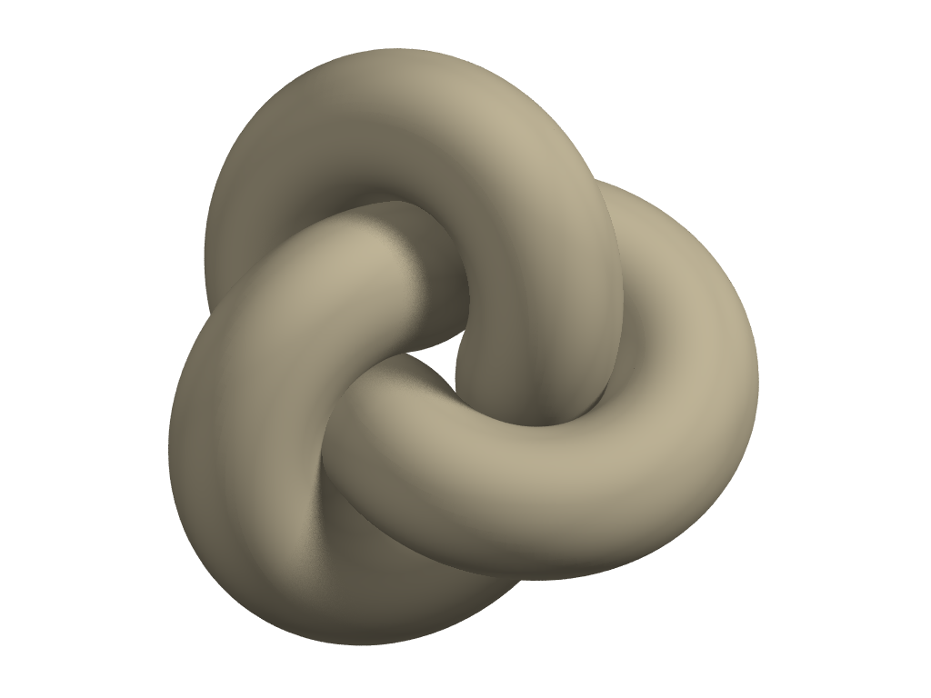
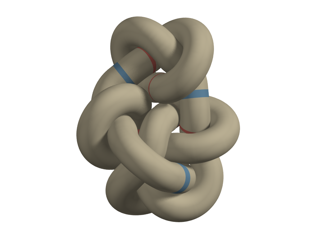
Figure 1: Tight configurations of $3_{1}$, $9_{48}^{m}$ and their connect sum $3_{1}\#9_{48}^{m}$. The sum of the writhes of the tight $3_{1}$ and $9_{48}^{m}$ configurations is $0.523$ while the writhe of the tight composite $3_{1}\#9_{48}^{m}$ is $0.625$. The difference is easily explained by looking at the pictures; in the connect sum, the lower left arc of the trefoil is spliced to the upper right arc of the $9_{48}^{m}$ shown above. The extra loop of the trefoil pushes the remainder of the knot out of its tight shape, changing the writhe of the overall composite. The other examples in our database look similar; in each case it seems that taking the connect sum and then tightening distorts one or both summands. Each of these configurations shows kinks (highlighted in red) and straight segments (highlighted in blue).

Composite knots which appear to violate the writhe conjecture

Knot	$\operatorname{Wr}(K_{1}\#K_{2})$	$\operatorname{Wr}(K_{1})+\operatorname{Wr}(K_{2})$	Difference (%)	# Start Positions
$3_{1}\#9_{48}^{m}$	0.523	0.625	19.412 %	13 (16,25)
$4_{1}\#7_{7}$	-0.534	-0.632	18.359 %	55 (25,331)
$3_{1}\#8_{14}^{m}$	0.556	0.634	14.127 %	50 (16,26)
$3_{1}\#8_{11}$	0.609	0.526	13.688 %	38 (16,21)
$3_{1}\#6_{2}^{m}$	-0.564	-0.632	12.000 %	17 (16,27)
$3_{1}\#8_{16}^{m}$	-0.576	-0.632	9.610 %	73 (16,23)
$3_{1}\#9_{45}^{m}$	1.711	1.865	8.979 %	16 (16,27)
$3_{1}\#9_{22}^{m}$	-1.123	-1.223	8.936 %	42 (16,24)
$5_{1}\#7_{2}$	-0.557	-0.606	8.810 %	109 (14,24)
$3_{1}\#9_{42}^{m}$	-2.197	-2.022	7.950 %	12 (16,24)
$3_{1}\#9_{21}^{m}$	1.197	1.110	7.236 %	92 (16,23)
$3_{1}\#8_{6}^{m}$	0.615	0.572	6.981 %	17 (16,22)
$3_{1}\#9_{12}^{m}$	1.171	1.092	6.782 %	83 (16,29)
$4_{1}\#8_{13}$	-1.116	-1.189	6.542 %	105 (25,21)
$5_{2}\#7_{4}^{m}$	1.170	1.234	5.420 %	21 (27,28)
$3_{1}\#5_{2}^{m}$	1.183	1.134	4.200 %	16 (16,27)
$5_{2}\#7_{5}^{m}$	2.771	2.886	4.130 %	98 (27,27)

Table 3: This table shows a selection of cases where the writhe conjecture is not supported by our data. The table shows the knot type, writhe of composite, sum of writhes of summands, absolute percentage difference between these numbers, and the number of start configurations tried for the composite (and in parentheses, the two summands). These are not the only cases where we are unable to verify the conjecture, but we have chosen not to show cases with more than two summands (because these more complicated knots simply may not be fully tightened), where the percentage difference was less than $4\%$, and where the writhe of the composite was less than $0.1$ (because in these cases a small absolute difference between writhes close to zero leads to huge percentage differences).

3.2 Ropelength of composite knots

Figure 2 shows a scatterplot of the ropelength of each of our composites ($x$-axis) plotted against the sum of the ropelengths of their prime summands. Katritch et al. [23] conjectured that the ropelength of the composite should be at least $4\pi-4$ less than the sum of the ropelength of the summands. This has become informally known as the connect sum conjecture for ropelength. The intuition behind the conjecture is easy to understand. When two pairs of linked rings (each with ropelength $8\pi$) are connect-summed to form a three link chain, the two rings which have been spliced together shrink to form a stadium curve with ropelength $4\pi+4$. The difference between the original ropelength of the rings ($8\pi$) and the ropelength of the stadium curve ($4\pi+4$) is the amount of rope saved in the splicing procedure: $4\pi-4$. For more complicated knots, it is somewhat surprising that the same amount of rope should be “exposed” to a connect sum. If this conjecture holds for very complicated knots, the principle at work would seem to be very different.

However, in this range of composite knots, our data suggests that the conjecture is quite plausible. In our dataset there are only 44 knots where our best conformation of the composite is very slightly longer than the conjecture predicts. In the most significant example of this phenomenon, the tightest $5_{1}^{m}\#7_{1}$ has ropelength $100.427$ while the conjecture predicts that there should be a conformation with ropelength $0.38\%$ lower ($\leq 100.042$).

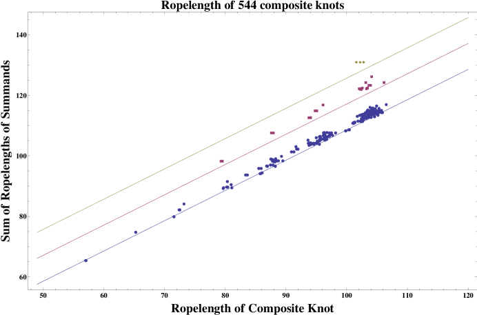
Figure 2: This scatterplot shows pairs $(x,y)$ where $x$ is the minimum ropelength we have found for a composite knot and $y$ is the sum of the minimum ropelengths we have found for its prime summands. On the plot, knots with two prime summands are plotted with blue circles, knots with three prime summands are plotted with red squares, and knots with four prime summands are plotted with yellow diamonds. According to the connect sum conjecture of [23], $y-x$ is at least $(N-1)(4\pi-4)$, where $N$ is the number of prime summands of the knot. This conjecture is shown by lines $y-x=4\pi-4$, $y-x=8\pi-8$, and $y-x=12\pi-12$. As one can see from the plot, all our data are very close to obeying the bounds predicted by the conjecture.

3.3 Other Observations about Tight Configurations

Table 4 shows the longest and shortest knots by crossing number for both prime and composite knots. We can see that the range of ropelengths for composite knots is smaller than the range for all knots of the same crossing number. One might expect composite knots to generally be longer than prime knots of the same crossing number since composites are separated in two pieces and have less opportunity to nest together and save rope. But it is mildly surprising that the longest knots of each crossing number are not composite. It will be interesting to see if this effect persists through higher crossing numbers.

Composite Knots

Prime Knots

$\operatorname{Cr}$ $\operatorname{Rop}$ Links $6$ $[57.042,57.073]$ $3_{1}\#3_{1}$, $3_{1}\#3_{1}^{m}$ $7$ $[65.240,65.240]$ $3_{1}\#4_{1}$, $3_{1}\#4_{1}$ $8$ $[71.544,73.193]$ $3_{1}\#5_{1}$, $4_{1}\#4_{1}$ $9$ $[79.329,81.088]$ $3_{1}\#3_{1}\#3_{1}$, $3_{1}\#6_{1}$ $10$ $[85.758,89.472]$ $3_{1}\#7_{1}$, $3_{1}\#7_{7}$ $11$ $[83.372,98.171]$ $3_{1}\#8_{19}^{m}$, $3_{1}\#8_{18}$ $12$ $[90.905,106.508]$ $3_{1}\#9_{46}$, $4_{1}\#8_{18}$

$\operatorname{Cr}$ $\operatorname{Rop}$ Knots $6$ $[56.7058,57.8392]$ $6_{1}$, $6_{3}$ $7$ $[61.4067,65.6924]$ $7_{1}$, $7_{6}$ $8$ $[60.9858,74.9063]$ $8_{19}$, $8_{18}$ $9$ $[68.6169,82.2803]$ $9_{46}$, $9_{33}$ $10$ $[71.0739,92.3565]$ $10_{124}$, $10_{123}$ $11$ (no data) $12$ (no data)

Table 4: Longest and shortest knots of a given crossing number for prime and composite knots. It is interesting to see that the longest and shortest knots of each crossing number are prime.

The embedded tube constraint is controlled by both tube-to-tube contacts (“struts”) and an upper bound on the curvature of the core polygon (“kinks”) [18, 33, 34]. It is a theorem (under some mild regularity assumptions) that no closed ropelength-critical curve can fail to have a strut [35], but kinks seem to be optional. However, in our data, tight configurations with kinks seem to be extremely common, occurring in 542 of our 544 composite configurations (although we expect that the two configurations without kinks have not fully converged). Another theorem is that sections of a ropelength-critical curve without struts or kinks are straight segments (see [35, 36] for different versions of this theorem). Gonzalez conjectured this phenomenon should occur in all tight composite knots with a mirror symmetry (such as the square knot in Figure 3). We find this phenomenon in 534 of the 544 composite knots with crossing number at most 12.

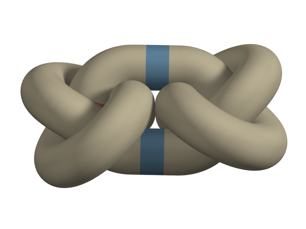
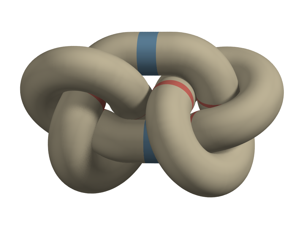
Figure 3: Two examples of tight composite knots. The left knot is an approximately tight configuration of the square knot $3_{1}\#3_{1}^{m}$ which shows the expected straight segments joining the two summands highlighted in blue. It is interesting that our tight configuration does not have a perfect geometric mirror symmetry (even though a critical configuration with this symmetry surely exists; see [37] for a discussion of symmetric criticality). The right knot is the approximately right granny knot $3_{1}\#3_{1}$. The ropelengths are $57.09$ and $57.05$, respectively.

4 Future Directions

Our publicly available dataset of tight knots and links, now including tight prime knots to 10 crossings, tight prime links to 9 crossings, and (with this paper) tight composite knots to 12 crossings should provide a substantial starting point for physicists, biologists, and mathematicians interested in the geometry of knotted configurations. We intend to expand the dataset to assemble tight configurations of all prime and composite knots and links to 12 crossings. This is a substantial undertaking even for prime knots and links, but the hardest part is certainly composite links. The problem is that composite links remain untabulated (it is still a challenging open problem to come up with an algorithm for tabulating composite links; see [30]).

It is certainly interesting that so many of our configurations exhibit “kinked” sections of maximum curvature. An excellent confirmation of this phenomenon would be to rerun our configurations with the curvature constraint removed to see whether we can achieve shorter lengths. In addition, the FEM techniques of Pieranski and Przybyl show great promise in computing at very high resolutions (up to tens of thousands of vertices). We intend to collaborate with this group for our next set of computations, using ridgerunner as a medium-resolution search tool to explore the configuration space of curves of a given knot type and then switching to FEM for the final tightening.

Acknowledgements. We are grateful to all the members of the UGA Geometry VIGRE group who contributed their time and effort towards this project. In particular, we would like to acknowledge the contributions of graduate students Ted Ashton and Steve Lane, who compiled the original table of composite knots, and Michael Piatek, who cowrote ridgerunner. We would also like to thank Piotr Pieranski and Sylwek Przybyl for checking our calculations. Our work was supported by the UGA VIGRE grants DMS-07-38586 and DMS-00-89927, UGA REU site grant DMS-06-49242, and NSF grants DMS-06-21903, DMS-08-10415, and DMS-11-15722 (to Rawdon).

References

Ropelength Tables

The pages that follow contain two sets of tables of ropelength data. The first set, Tables 5-10 on pages 5–10, show the polygonal ropelength ($\operatorname{Rop}_{p}$) and ropelength upper bounds ($\operatorname{Rop}$) that we have obtained for each of the composite knot types that we have considered. The composite knots are organized by dictionary order on their summands, with the primary order coming from position in Rolfsen’s table [28], with the knot $X^{y}_{z}$ being the $z$-th example of a prime $X$-crossing link of $y$ components in the table. Knots with the same Rolfsen position are ordered by symmetry type, with the convention $K<K^{m}<K^{r}<K^{rm}$. To aid the reader in making sense of the table, we insert lines where the crossing number changes and spaces where the base types of the summands change.

The second set of tables, Tables 11–16 on pages 11–16 give the residual of each of our computed configurations. The low residuals show that they are close to critical. We include this data as a measure of the relative quality of each of our minimized configurations.

Table 5: Ropelengths of Tight Knots by Knot Type, Part 1 of 6

Knot	$\operatorname{Rop}_{p}$	$\operatorname{Rop}$
$3_{1}\#3_{1}$	$57.05$	$57.04$
$3_{1}\#3_{1}^{m}$	$57.09$	$57.07$
$3_{1}^{m}\#3_{1}^{m}$	$57.05$	$57.04$
$3_{1}\#4_{1}$	$65.26$	$65.24$
$3_{1}^{m}\#4_{1}$	$65.26$	$65.24$
$3_{1}\#5_{1}$	$71.56$	$71.54$
$3_{1}\#5_{1}^{m}$	$71.59$	$71.58$
$3_{1}^{m}\#5_{1}$	$71.59$	$71.58$
$3_{1}^{m}\#5_{1}^{m}$	$71.56$	$71.54$
$3_{1}\#5_{2}$	$72.43$	$72.41$
$3_{1}\#5_{2}^{m}$	$72.55$	$72.53$
$3_{1}^{m}\#5_{2}$	$72.55$	$72.53$
$3_{1}^{m}\#5_{2}^{m}$	$72.43$	$72.41$
$4_{1}\#4_{1}$	$73.20$	$73.19$
$3_{1}\#6_{1}$	$81.10$	$81.09$
$3_{1}\#6_{1}^{m}$	$79.73$	$79.72$
$3_{1}^{m}\#6_{1}$	$79.73$	$79.72$
$3_{1}^{m}\#6_{1}^{m}$	$81.10$	$81.09$
$3_{1}\#6_{2}$	$80.27$	$80.25$
$3_{1}\#6_{2}^{m}$	$80.43$	$80.42$
$3_{1}^{m}\#6_{2}$	$80.43$	$80.42$
$3_{1}^{m}\#6_{2}^{m}$	$80.27$	$80.25$
$3_{1}\#6_{3}$	$81.02$	$81.00$
$3_{1}^{m}\#6_{3}$	$81.02$	$81.00$
$4_{1}\#5_{1}$	$79.67$	$79.65$
$4_{1}\#5_{1}^{m}$	$79.67$	$79.65$
$4_{1}\#5_{2}$	$80.36$	$80.34$
$4_{1}\#5_{2}^{m}$	$80.36$	$80.34$

Knot	$\operatorname{Rop}_{p}$	$\operatorname{Rop}$
$3_{1}\#3_{1}\#3_{1}$	$79.35$	$79.33$
$3_{1}\#3_{1}\#3_{1}^{m}$	$79.57$	$79.56$
$3_{1}\#3_{1}^{m}\#3_{1}^{m}$	$79.57$	$79.56$
$3_{1}^{m}\#3_{1}^{m}\#3_{1}^{m}$	$79.35$	$79.33$
$3_{1}\#7_{1}$	$85.78$	$85.76$
$3_{1}\#7_{1}^{m}$	$85.82$	$85.80$
$3_{1}^{m}\#7_{1}$	$85.82$	$85.80$
$3_{1}^{m}\#7_{1}^{m}$	$85.78$	$85.76$
$3_{1}\#7_{2}$	$86.98$	$86.96$
$3_{1}\#7_{2}^{m}$	$88.24$	$88.22$
$3_{1}^{m}\#7_{2}$	$88.24$	$88.22$
$3_{1}^{m}\#7_{2}^{m}$	$86.98$	$86.96$
$3_{1}\#7_{3}$	$88.27$	$88.25$
$3_{1}\#7_{3}^{m}$	$86.94$	$86.92$
$3_{1}^{m}\#7_{3}$	$86.94$	$86.92$
$3_{1}^{m}\#7_{3}^{m}$	$88.27$	$88.25$
$3_{1}\#7_{4}$	$87.85$	$87.84$
$3_{1}\#7_{4}^{m}$	$87.48$	$87.46$
$3_{1}^{m}\#7_{4}$	$87.48$	$87.46$
$3_{1}^{m}\#7_{4}^{m}$	$87.85$	$87.84$
$3_{1}\#7_{5}$	$88.22$	$88.20$
$3_{1}\#7_{5}^{m}$	$88.09$	$88.07$
$3_{1}^{m}\#7_{5}$	$88.09$	$88.07$
$3_{1}^{m}\#7_{5}^{m}$	$88.22$	$88.20$
$3_{1}\#7_{6}$	$88.57$	$88.55$
$3_{1}\#7_{6}^{m}$	$88.45$	$88.43$
$3_{1}^{m}\#7_{6}$	$88.45$	$88.43$
$3_{1}^{m}\#7_{6}^{m}$	$88.57$	$88.55$
$3_{1}\#7_{7}$	$89.49$	$89.47$
$3_{1}\#7_{7}^{m}$	$88.77$	$88.75$
$3_{1}^{m}\#7_{7}$	$88.77$	$88.75$

Knot	$\operatorname{Rop}_{p}$	$\operatorname{Rop}$
$3_{1}^{m}\#7_{7}^{m}$	$89.49$	$89.47$
$4_{1}\#6_{1}$	$87.88$	$87.86$
$4_{1}\#6_{1}^{m}$	$87.88$	$87.86$
$4_{1}\#6_{2}$	$88.31$	$88.29$
$4_{1}\#6_{2}^{m}$	$88.31$	$88.29$
$4_{1}\#6_{3}$	$89.31$	$89.29$
$5_{1}\#5_{1}$	$86.06$	$86.03$
$5_{1}\#5_{1}^{m}$	$86.11$	$86.09$
$5_{1}^{m}\#5_{1}^{m}$	$86.06$	$86.03$
$5_{1}\#5_{2}$	$86.82$	$86.80$
$5_{1}\#5_{2}^{m}$	$86.97$	$86.95$
$5_{1}^{m}\#5_{2}$	$86.97$	$86.95$
$5_{1}^{m}\#5_{2}^{m}$	$86.82$	$86.80$
$5_{2}\#5_{2}$	$87.52$	$87.51$
$5_{2}\#5_{2}^{m}$	$87.61$	$87.60$
$5_{2}^{m}\#5_{2}^{m}$	$87.52$	$87.51$
$3_{1}\#3_{1}\#4_{1}$	$87.63$	$87.61$
$3_{1}\#3_{1}^{m}\#4_{1}$	$87.94$	$87.92$
$3_{1}^{m}\#3_{1}^{m}\#4_{1}$	$87.63$	$87.61$
$3_{1}\#8_{1}$	$93.92$	$93.90$
$3_{1}\#8_{1}^{m}$	$94.06$	$94.04$
$3_{1}^{m}\#8_{1}$	$94.06$	$94.04$
$3_{1}^{m}\#8_{1}^{m}$	$93.92$	$93.90$
$3_{1}\#8_{2}$	$94.42$	$94.40$
$3_{1}\#8_{2}^{m}$	$94.68$	$94.66$
$3_{1}^{m}\#8_{2}$	$94.68$	$94.66$
$3_{1}^{m}\#8_{2}^{m}$	$94.42$	$94.40$
$3_{1}\#8_{3}$	$95.53$	$95.50$
$3_{1}^{m}\#8_{3}$	$95.53$	$95.50$

Table 6: Ropelengths of Tight Knots by Knot Type, Part 2 of 6

Knot	$\operatorname{Rop}_{p}$	$\operatorname{Rop}$
$3_{1}\#8_{4}$	$94.63$	$94.61$
$3_{1}\#8_{4}^{m}$	$94.98$	$94.96$
$3_{1}^{m}\#8_{4}$	$94.98$	$94.96$
$3_{1}^{m}\#8_{4}^{m}$	$94.63$	$94.61$
$3_{1}\#8_{5}$	$95.20$	$95.18$
$3_{1}\#8_{5}^{m}$	$95.40$	$95.38$
$3_{1}^{m}\#8_{5}$	$95.40$	$95.38$
$3_{1}^{m}\#8_{5}^{m}$	$95.20$	$95.18$
$3_{1}\#8_{6}$	$95.62$	$95.59$
$3_{1}\#8_{6}^{m}$	$95.64$	$95.62$
$3_{1}^{m}\#8_{6}$	$95.64$	$95.62$
$3_{1}^{m}\#8_{6}^{m}$	$95.62$	$95.59$
$3_{1}\#8_{7}$	$95.48$	$95.47$
$3_{1}\#8_{7}^{m}$	$95.62$	$95.59$
$3_{1}^{m}\#8_{7}$	$95.62$	$95.59$
$3_{1}^{m}\#8_{7}^{m}$	$95.48$	$95.47$
$3_{1}\#8_{8}$	$96.94$	$96.69$
$3_{1}\#8_{8}^{m}$	$95.58$	$95.56$
$3_{1}^{m}\#8_{8}$	$95.58$	$95.56$
$3_{1}^{m}\#8_{8}^{m}$	$96.94$	$96.69$
$3_{1}\#8_{9}$	$96.47$	$96.45$
$3_{1}^{m}\#8_{9}$	$96.47$	$96.45$
$3_{1}\#8_{10}$	$96.22$	$96.20$
$3_{1}\#8_{10}^{m}$	$96.65$	$96.63$
$3_{1}^{m}\#8_{10}$	$96.65$	$96.63$
$3_{1}^{m}\#8_{10}^{m}$	$96.22$	$96.20$
$3_{1}\#8_{11}$	$95.70$	$95.68$
$3_{1}\#8_{11}^{m}$	$95.64$	$95.62$
$3_{1}^{m}\#8_{11}$	$95.64$	$95.62$
$3_{1}^{m}\#8_{11}^{m}$	$95.70$	$95.68$
$3_{1}\#8_{12}$	$96.48$	$96.47$

Knot	$\operatorname{Rop}_{p}$	$\operatorname{Rop}$
$3_{1}^{m}\#8_{12}$	$96.48$	$96.47$
$3_{1}\#8_{13}$	$96.44$	$96.42$
$3_{1}\#8_{13}^{m}$	$96.02$	$95.99$
$3_{1}^{m}\#8_{13}$	$96.02$	$95.99$
$3_{1}^{m}\#8_{13}^{m}$	$96.44$	$96.42$
$3_{1}\#8_{14}$	$97.19$	$97.17$
$3_{1}\#8_{14}^{m}$	$97.03$	$97.00$
$3_{1}^{m}\#8_{14}$	$97.03$	$97.00$
$3_{1}^{m}\#8_{14}^{m}$	$97.19$	$97.17$
$3_{1}\#8_{15}$	$96.54$	$96.52$
$3_{1}\#8_{15}^{m}$	$96.33$	$96.31$
$3_{1}^{m}\#8_{15}$	$96.33$	$96.31$
$3_{1}^{m}\#8_{15}^{m}$	$96.54$	$96.52$
$3_{1}\#8_{16}$	$96.51$	$96.50$
$3_{1}\#8_{16}^{m}$	$96.84$	$96.82$
$3_{1}^{m}\#8_{16}$	$96.84$	$96.82$
$3_{1}^{m}\#8_{16}^{m}$	$96.51$	$96.50$
$3_{1}\#8_{17}$	$97.44$	$97.41$
$3_{1}\#8_{17}^{r}$	$97.44$	$97.41$
$3_{1}^{m}\#8_{17}$	$97.44$	$97.41$
$3_{1}^{m}\#8_{17}^{r}$	$97.44$	$97.41$
$3_{1}\#8_{18}$	$98.19$	$98.17$
$3_{1}^{m}\#8_{18}$	$98.19$	$98.17$
$3_{1}\#8_{19}$	$83.68$	$83.67$
$3_{1}\#8_{19}^{m}$	$83.39$	$83.37$
$3_{1}^{m}\#8_{19}$	$83.39$	$83.37$
$3_{1}^{m}\#8_{19}^{m}$	$83.68$	$83.67$
$3_{1}\#8_{20}$	$85.55$	$85.53$
$3_{1}\#8_{20}^{m}$	$85.95$	$85.94$
$3_{1}^{m}\#8_{20}$	$85.95$	$85.94$
$3_{1}^{m}\#8_{20}^{m}$	$85.55$	$85.53$

Knot	$\operatorname{Rop}_{p}$	$\operatorname{Rop}$
$3_{1}\#8_{21}$	$87.81$	$87.79$
$3_{1}\#8_{21}^{m}$	$88.01$	$87.99$
$3_{1}^{m}\#8_{21}$	$88.01$	$87.99$
$3_{1}^{m}\#8_{21}^{m}$	$87.81$	$87.79$
$4_{1}\#7_{1}$	$93.83$	$93.81$
$4_{1}\#7_{1}^{m}$	$93.83$	$93.81$
$4_{1}\#7_{2}$	$96.31$	$96.29$
$4_{1}\#7_{2}^{m}$	$96.31$	$96.29$
$4_{1}\#7_{3}$	$95.04$	$95.02$
$4_{1}\#7_{3}^{m}$	$95.04$	$95.02$
$4_{1}\#7_{4}$	$95.56$	$95.54$
$4_{1}\#7_{4}^{m}$	$95.56$	$95.54$
$4_{1}\#7_{5}$	$96.37$	$96.35$
$4_{1}\#7_{5}^{m}$	$96.37$	$96.35$
$4_{1}\#7_{6}$	$96.35$	$96.33$
$4_{1}\#7_{6}^{m}$	$96.35$	$96.33$
$4_{1}\#7_{7}$	$96.76$	$96.75$
$4_{1}\#7_{7}^{m}$	$96.76$	$96.75$
$5_{1}\#6_{1}$	$94.62$	$94.61$
$5_{1}\#6_{1}^{m}$	$94.17$	$94.14$
$5_{1}^{m}\#6_{1}$	$94.17$	$94.14$
$5_{1}^{m}\#6_{1}^{m}$	$94.62$	$94.61$
$5_{1}\#6_{2}$	$94.58$	$94.56$
$5_{1}\#6_{2}^{m}$	$95.19$	$95.17$
$5_{1}^{m}\#6_{2}$	$95.19$	$95.17$
$5_{1}^{m}\#6_{2}^{m}$	$94.58$	$94.56$
$5_{1}\#6_{3}$	$95.43$	$95.41$
$5_{1}^{m}\#6_{3}$	$95.43$	$95.41$
$5_{2}\#6_{1}$	$95.73$	$95.71$
$5_{2}\#6_{1}^{m}$	$96.36$	$96.34$

Table 7: Ropelengths of Tight Knots by Knot Type, Part 3 of 6

Knot	$\operatorname{Rop}_{p}$	$\operatorname{Rop}$
$5_{2}^{m}\#6_{1}$	$96.36$	$96.34$
$5_{2}^{m}\#6_{1}^{m}$	$95.73$	$95.71$
$5_{2}\#6_{2}$	$96.56$	$96.55$
$5_{2}\#6_{2}^{m}$	$95.64$	$95.62$
$5_{2}^{m}\#6_{2}$	$95.64$	$95.62$
$5_{2}^{m}\#6_{2}^{m}$	$96.56$	$96.55$
$5_{2}\#6_{3}$	$96.32$	$96.30$
$5_{2}^{m}\#6_{3}$	$96.32$	$96.30$
$3_{1}\#3_{1}\#5_{1}$	$93.79$	$93.77$
$3_{1}\#3_{1}\#5_{1}^{m}$	$94.12$	$94.10$
$3_{1}\#3_{1}^{m}\#5_{1}$	$94.08$	$94.06$
$3_{1}\#3_{1}^{m}\#5_{1}^{m}$	$94.08$	$94.06$
$3_{1}^{m}\#3_{1}^{m}\#5_{1}$	$94.12$	$94.10$
$3_{1}^{m}\#3_{1}^{m}\#5_{1}^{m}$	$93.79$	$93.77$
$3_{1}\#3_{1}\#5_{2}$	$94.81$	$94.79$
$3_{1}\#3_{1}\#5_{2}^{m}$	$95.04$	$95.02$
$3_{1}\#3_{1}^{m}\#5_{2}$	$95.13$	$95.08$
$3_{1}\#3_{1}^{m}\#5_{2}^{m}$	$95.13$	$95.08$
$3_{1}^{m}\#3_{1}^{m}\#5_{2}$	$95.04$	$95.02$
$3_{1}^{m}\#3_{1}^{m}\#5_{2}^{m}$	$94.81$	$94.79$
$3_{1}\#4_{1}\#4_{1}$	$96.15$	$96.13$
$3_{1}^{m}\#4_{1}\#4_{1}$	$96.15$	$96.13$
$3_{1}\#9_{1}$	$99.88$	$99.86$
$3_{1}\#9_{1}^{m}$	$99.90$	$99.88$
$3_{1}^{m}\#9_{1}$	$99.90$	$99.88$
$3_{1}^{m}\#9_{1}^{m}$	$99.88$	$99.86$
$3_{1}\#9_{2}$	$101.10$	$101.08$
$3_{1}\#9_{2}^{m}$	$101.20$	$101.17$
$3_{1}^{m}\#9_{2}$	$101.20$	$101.17$
$3_{1}^{m}\#9_{2}^{m}$	$101.10$	$101.08$

Knot	$\operatorname{Rop}_{p}$	$\operatorname{Rop}$
$3_{1}\#9_{3}$	$101.23$	$101.21$
$3_{1}\#9_{3}^{m}$	$101.27$	$101.25$
$3_{1}^{m}\#9_{3}$	$101.27$	$101.25$
$3_{1}^{m}\#9_{3}^{m}$	$101.23$	$101.21$
$3_{1}\#9_{4}$	$101.32$	$101.30$
$3_{1}\#9_{4}^{m}$	$101.36$	$101.34$
$3_{1}^{m}\#9_{4}$	$101.36$	$101.34$
$3_{1}^{m}\#9_{4}^{m}$	$101.32$	$101.30$
$3_{1}\#9_{5}$	$102.61$	$102.58$
$3_{1}\#9_{5}^{m}$	$102.40$	$102.37$
$3_{1}^{m}\#9_{5}$	$102.40$	$102.37$
$3_{1}^{m}\#9_{5}^{m}$	$102.61$	$102.58$
$3_{1}\#9_{6}$	$102.48$	$102.45$
$3_{1}\#9_{6}^{m}$	$102.64$	$102.61$
$3_{1}^{m}\#9_{6}$	$102.64$	$102.61$
$3_{1}^{m}\#9_{6}^{m}$	$102.48$	$102.45$
$3_{1}\#9_{7}$	$103.28$	$103.26$
$3_{1}\#9_{7}^{m}$	$102.67$	$102.65$
$3_{1}^{m}\#9_{7}$	$102.67$	$102.65$
$3_{1}^{m}\#9_{7}^{m}$	$103.28$	$103.26$
$3_{1}\#9_{8}$	$102.80$	$102.78$
$3_{1}\#9_{8}^{m}$	$103.00$	$102.98$
$3_{1}^{m}\#9_{8}$	$103.00$	$102.98$
$3_{1}^{m}\#9_{8}^{m}$	$102.80$	$102.78$
$3_{1}\#9_{9}$	$102.66$	$102.63$
$3_{1}\#9_{9}^{m}$	$102.78$	$102.75$
$3_{1}^{m}\#9_{9}$	$102.78$	$102.75$
$3_{1}^{m}\#9_{9}^{m}$	$102.66$	$102.63$
$3_{1}\#9_{10}$	$102.82$	$102.79$
$3_{1}\#9_{10}^{m}$	$103.05$	$103.03$
$3_{1}^{m}\#9_{10}$	$103.05$	$103.03$

Knot	$\operatorname{Rop}_{p}$	$\operatorname{Rop}$
$3_{1}^{m}\#9_{10}^{m}$	$102.82$	$102.79$
$3_{1}\#9_{11}$	$102.92$	$102.90$
$3_{1}\#9_{11}^{m}$	$102.81$	$102.78$
$3_{1}^{m}\#9_{11}$	$102.81$	$102.78$
$3_{1}^{m}\#9_{11}^{m}$	$102.92$	$102.90$
$3_{1}\#9_{12}$	$103.70$	$103.67$
$3_{1}\#9_{12}^{m}$	$102.93$	$102.91$
$3_{1}^{m}\#9_{12}$	$102.93$	$102.91$
$3_{1}^{m}\#9_{12}^{m}$	$103.70$	$103.67$
$3_{1}\#9_{13}$	$104.61$	$104.59$
$3_{1}\#9_{13}^{m}$	$104.59$	$104.57$
$3_{1}^{m}\#9_{13}$	$104.59$	$104.57$
$3_{1}^{m}\#9_{13}^{m}$	$104.61$	$104.59$
$3_{1}\#9_{14}$	$103.58$	$103.56$
$3_{1}\#9_{14}^{m}$	$103.21$	$103.19$
$3_{1}^{m}\#9_{14}$	$103.21$	$103.19$
$3_{1}^{m}\#9_{14}^{m}$	$103.58$	$103.56$
$3_{1}\#9_{15}$	$103.61$	$103.58$
$3_{1}\#9_{15}^{m}$	$103.56$	$103.54$
$3_{1}^{m}\#9_{15}$	$103.56$	$103.54$
$3_{1}^{m}\#9_{15}^{m}$	$103.61$	$103.58$
$3_{1}\#9_{16}$	$103.32$	$103.29$
$3_{1}\#9_{16}^{m}$	$103.87$	$103.85$
$3_{1}^{m}\#9_{16}$	$103.87$	$103.85$
$3_{1}^{m}\#9_{16}^{m}$	$103.32$	$103.29$
$3_{1}\#9_{17}$	$103.02$	$103.00$
$3_{1}\#9_{17}^{m}$	$103.65$	$103.62$
$3_{1}^{m}\#9_{17}$	$103.65$	$103.62$
$3_{1}^{m}\#9_{17}^{m}$	$103.02$	$103.00$
$3_{1}\#9_{18}$	$103.77$	$103.75$
$3_{1}\#9_{18}^{m}$	$103.83$	$103.80$

Table 8: Ropelengths of Tight Knots by Knot Type, Part 4 of 6

Knot	$\operatorname{Rop}_{p}$	$\operatorname{Rop}$
$3_{1}^{m}\#9_{18}$	$103.83$	$103.80$
$3_{1}^{m}\#9_{18}^{m}$	$103.77$	$103.75$
$3_{1}\#9_{19}$	$103.57$	$103.55$
$3_{1}\#9_{19}^{m}$	$104.08$	$104.06$
$3_{1}^{m}\#9_{19}$	$104.08$	$104.06$
$3_{1}^{m}\#9_{19}^{m}$	$103.57$	$103.55$
$3_{1}\#9_{20}$	$103.67$	$103.65$
$3_{1}\#9_{20}^{m}$	$103.42$	$103.39$
$3_{1}^{m}\#9_{20}$	$103.42$	$103.39$
$3_{1}^{m}\#9_{20}^{m}$	$103.67$	$103.65$
$3_{1}\#9_{21}$	$103.83$	$103.81$
$3_{1}\#9_{21}^{m}$	$103.84$	$103.82$
$3_{1}^{m}\#9_{21}$	$103.84$	$103.82$
$3_{1}^{m}\#9_{21}^{m}$	$103.83$	$103.81$
$3_{1}\#9_{22}$	$103.97$	$103.94$
$3_{1}\#9_{22}^{m}$	$104.12$	$104.09$
$3_{1}^{m}\#9_{22}$	$104.12$	$104.09$
$3_{1}^{m}\#9_{22}^{m}$	$103.97$	$103.94$
$3_{1}\#9_{23}$	$104.59$	$104.56$
$3_{1}\#9_{23}^{m}$	$104.20$	$104.18$
$3_{1}^{m}\#9_{23}$	$104.20$	$104.18$
$3_{1}^{m}\#9_{23}^{m}$	$104.59$	$104.56$
$3_{1}\#9_{24}$	$104.50$	$104.48$
$3_{1}\#9_{24}^{m}$	$103.93$	$103.91$
$3_{1}^{m}\#9_{24}$	$103.93$	$103.91$
$3_{1}^{m}\#9_{24}^{m}$	$104.50$	$104.48$
$3_{1}\#9_{25}$	$104.13$	$104.11$
$3_{1}\#9_{25}^{m}$	$103.94$	$103.92$
$3_{1}^{m}\#9_{25}$	$103.94$	$103.92$
$3_{1}^{m}\#9_{25}^{m}$	$104.13$	$104.11$
$3_{1}\#9_{26}$	$104.28$	$104.25$

Knot	$\operatorname{Rop}_{p}$	$\operatorname{Rop}$
$3_{1}\#9_{26}^{m}$	$104.21$	$104.18$
$3_{1}^{m}\#9_{26}$	$104.21$	$104.18$
$3_{1}^{m}\#9_{26}^{m}$	$104.28$	$104.25$
$3_{1}\#9_{27}$	$104.98$	$104.95$
$3_{1}\#9_{27}^{m}$	$104.47$	$104.44$
$3_{1}^{m}\#9_{27}$	$104.47$	$104.44$
$3_{1}^{m}\#9_{27}^{m}$	$104.98$	$104.95$
$3_{1}\#9_{28}$	$104.25$	$104.23$
$3_{1}\#9_{28}^{m}$	$104.52$	$104.50$
$3_{1}^{m}\#9_{28}$	$104.52$	$104.50$
$3_{1}^{m}\#9_{28}^{m}$	$104.25$	$104.23$
$3_{1}\#9_{29}$	$104.13$	$104.11$
$3_{1}\#9_{29}^{m}$	$104.97$	$104.94$
$3_{1}^{m}\#9_{29}$	$104.97$	$104.94$
$3_{1}^{m}\#9_{29}^{m}$	$104.13$	$104.11$
$3_{1}\#9_{30}$	$104.39$	$104.36$
$3_{1}\#9_{30}^{m}$	$104.20$	$104.18$
$3_{1}^{m}\#9_{30}$	$104.20$	$104.18$
$3_{1}^{m}\#9_{30}^{m}$	$104.39$	$104.36$
$3_{1}\#9_{31}$	$104.80$	$104.78$
$3_{1}\#9_{31}^{m}$	$105.35$	$105.33$
$3_{1}^{m}\#9_{31}$	$105.35$	$105.33$
$3_{1}^{m}\#9_{31}^{m}$	$104.80$	$104.78$
$3_{1}\#9_{32}$	$104.64$	$104.62$
$3_{1}\#9_{32}^{r}$	$104.64$	$104.62$
$3_{1}\#9_{32}^{m}$	$104.60$	$104.58$
$3_{1}\#9_{32}^{rm}$	$104.60$	$104.58$
$3_{1}^{m}\#9_{32}$	$104.60$	$104.58$
$3_{1}^{m}\#9_{32}^{r}$	$104.60$	$104.58$
$3_{1}^{m}\#9_{32}^{m}$	$104.64$	$104.62$
$3_{1}^{m}\#9_{32}^{rm}$	$104.64$	$104.62$

Knot	$\operatorname{Rop}_{p}$	$\operatorname{Rop}$
$3_{1}\#9_{33}$	$105.77$	$105.74$
$3_{1}\#9_{33}^{r}$	$105.77$	$105.74$
$3_{1}\#9_{33}^{m}$	$104.86$	$104.83$
$3_{1}\#9_{33}^{rm}$	$104.86$	$104.83$
$3_{1}^{m}\#9_{33}$	$104.86$	$104.83$
$3_{1}^{m}\#9_{33}^{r}$	$104.86$	$104.83$
$3_{1}^{m}\#9_{33}^{m}$	$105.77$	$105.74$
$3_{1}^{m}\#9_{33}^{rm}$	$105.77$	$105.74$
$3_{1}\#9_{34}$	$105.07$	$105.05$
$3_{1}\#9_{34}^{m}$	$105.62$	$105.60$
$3_{1}^{m}\#9_{34}$	$105.62$	$105.60$
$3_{1}^{m}\#9_{34}^{m}$	$105.07$	$105.05$
$3_{1}\#9_{35}$	$102.44$	$102.42$
$3_{1}\#9_{35}^{m}$	$102.82$	$102.80$
$3_{1}^{m}\#9_{35}$	$102.82$	$102.80$
$3_{1}^{m}\#9_{35}^{m}$	$102.44$	$102.42$
$3_{1}\#9_{36}$	$103.90$	$103.87$
$3_{1}\#9_{36}^{m}$	$103.40$	$103.38$
$3_{1}^{m}\#9_{36}$	$103.40$	$103.38$
$3_{1}^{m}\#9_{36}^{m}$	$103.90$	$103.87$
$3_{1}\#9_{37}$	$103.54$	$103.52$
$3_{1}\#9_{37}^{m}$	$103.75$	$103.73$
$3_{1}^{m}\#9_{37}$	$103.75$	$103.73$
$3_{1}^{m}\#9_{37}^{m}$	$103.54$	$103.52$
$3_{1}\#9_{38}$	$104.63$	$104.61$
$3_{1}\#9_{38}^{m}$	$104.76$	$104.74$
$3_{1}^{m}\#9_{38}$	$104.76$	$104.74$
$3_{1}^{m}\#9_{38}^{m}$	$104.63$	$104.61$
$3_{1}\#9_{39}$	$104.53$	$104.51$
$3_{1}\#9_{39}^{m}$	$104.85$	$104.83$
$3_{1}^{m}\#9_{39}$	$104.85$	$104.83$

Table 9: Ropelengths of Tight Knots by Knot Type, Part 5 of 6

Knot	$\operatorname{Rop}_{p}$	$\operatorname{Rop}$
$3_{1}^{m}\#9_{39}^{m}$	$104.53$	$104.51$
$3_{1}\#9_{40}$	$105.91$	$105.89$
$3_{1}\#9_{40}^{m}$	$105.76$	$105.74$
$3_{1}^{m}\#9_{40}$	$105.76$	$105.74$
$3_{1}^{m}\#9_{40}^{m}$	$105.91$	$105.89$
$3_{1}\#9_{41}$	$104.67$	$104.65$
$3_{1}\#9_{41}^{m}$	$104.39$	$104.37$
$3_{1}^{m}\#9_{41}$	$104.39$	$104.37$
$3_{1}^{m}\#9_{41}^{m}$	$104.67$	$104.65$
$3_{1}\#9_{42}$	$92.02$	$92.00$
$3_{1}\#9_{42}^{m}$	$91.79$	$91.77$
$3_{1}^{m}\#9_{42}$	$91.79$	$91.77$
$3_{1}^{m}\#9_{42}^{m}$	$92.02$	$92.00$
$3_{1}\#9_{43}$	$93.70$	$93.69$
$3_{1}\#9_{43}^{m}$	$93.81$	$93.78$
$3_{1}^{m}\#9_{43}$	$93.81$	$93.78$
$3_{1}^{m}\#9_{43}^{m}$	$93.70$	$93.69$
$3_{1}\#9_{44}$	$93.86$	$93.84$
$3_{1}\#9_{44}^{m}$	$94.10$	$94.08$
$3_{1}^{m}\#9_{44}$	$94.10$	$94.08$
$3_{1}^{m}\#9_{44}^{m}$	$93.86$	$93.84$
$3_{1}\#9_{45}$	$97.26$	$97.24$
$3_{1}\#9_{45}^{m}$	$97.71$	$97.69$
$3_{1}^{m}\#9_{45}$	$97.71$	$97.69$
$3_{1}^{m}\#9_{45}^{m}$	$97.26$	$97.24$
$3_{1}\#9_{46}$	$90.93$	$90.91$
$3_{1}\#9_{46}^{m}$	$91.33$	$91.31$
$3_{1}^{m}\#9_{46}$	$91.33$	$91.31$
$3_{1}^{m}\#9_{46}^{m}$	$90.93$	$90.91$
$3_{1}\#9_{47}$	$97.55$	$97.51$
$3_{1}\#9_{47}^{m}$	$97.17$	$97.15$

Knot	$\operatorname{Rop}_{p}$	$\operatorname{Rop}$
$3_{1}^{m}\#9_{47}$	$97.17$	$97.15$
$3_{1}^{m}\#9_{47}^{m}$	$97.55$	$97.51$
$3_{1}\#9_{48}$	$97.13$	$97.11$
$3_{1}\#9_{48}^{m}$	$96.50$	$96.47$
$3_{1}^{m}\#9_{48}$	$96.50$	$96.47$
$3_{1}^{m}\#9_{48}^{m}$	$97.13$	$97.11$
$3_{1}\#9_{49}$	$96.29$	$96.27$
$3_{1}\#9_{49}^{m}$	$96.17$	$96.16$
$3_{1}^{m}\#9_{49}$	$96.17$	$96.16$
$3_{1}^{m}\#9_{49}^{m}$	$96.29$	$96.27$
$4_{1}\#8_{1}$	$101.81$	$101.78$
$4_{1}\#8_{1}^{m}$	$101.81$	$101.78$
$4_{1}\#8_{2}$	$102.44$	$102.42$
$4_{1}\#8_{2}^{m}$	$102.44$	$102.42$
$4_{1}\#8_{3}$	$103.69$	$103.67$
$4_{1}\#8_{4}$	$102.78$	$102.76$
$4_{1}\#8_{4}^{m}$	$102.78$	$102.76$
$4_{1}\#8_{5}$	$103.09$	$103.07$
$4_{1}\#8_{5}^{m}$	$103.09$	$103.07$
$4_{1}\#8_{6}$	$103.47$	$103.45$
$4_{1}\#8_{6}^{m}$	$103.47$	$103.45$
$4_{1}\#8_{7}$	$103.55$	$103.53$
$4_{1}\#8_{7}^{m}$	$103.55$	$103.53$
$4_{1}\#8_{8}$	$103.50$	$103.48$
$4_{1}\#8_{8}^{m}$	$103.50$	$103.48$
$4_{1}\#8_{9}$	$103.94$	$103.93$
$4_{1}\#8_{10}$	$104.42$	$104.40$
$4_{1}\#8_{10}^{m}$	$104.42$	$104.40$
$4_{1}\#8_{11}$	$103.76$	$103.74$

Knot	$\operatorname{Rop}_{p}$	$\operatorname{Rop}$
$4_{1}\#8_{11}^{m}$	$103.76$	$103.74$
$4_{1}\#8_{12}$	$103.87$	$103.84$
$4_{1}\#8_{13}$	$104.19$	$104.17$
$4_{1}\#8_{13}^{m}$	$104.19$	$104.17$
$4_{1}\#8_{14}$	$104.33$	$104.30$
$4_{1}\#8_{14}^{m}$	$104.33$	$104.30$
$4_{1}\#8_{15}$	$104.23$	$104.21$
$4_{1}\#8_{15}^{m}$	$104.23$	$104.21$
$4_{1}\#8_{16}$	$104.74$	$104.71$
$4_{1}\#8_{16}^{m}$	$104.74$	$104.71$
$4_{1}\#8_{17}$	$104.96$	$104.94$
$4_{1}\#8_{17}^{r}$	$104.96$	$104.94$
$4_{1}\#8_{18}$	$106.53$	$106.51$
$4_{1}\#8_{19}$	$91.64$	$91.62$
$4_{1}\#8_{19}^{m}$	$91.64$	$91.62$
$4_{1}\#8_{20}$	$93.64$	$93.62$
$4_{1}\#8_{20}^{m}$	$93.64$	$93.62$
$4_{1}\#8_{21}$	$96.20$	$96.19$
$4_{1}\#8_{21}^{m}$	$96.20$	$96.19$
$5_{1}\#7_{1}$	$100.38$	$100.36$
$5_{1}\#7_{1}^{m}$	$100.45$	$100.43$
$5_{1}^{m}\#7_{1}$	$100.45$	$100.43$
$5_{1}^{m}\#7_{1}^{m}$	$100.38$	$100.36$
$5_{1}\#7_{2}$	$101.30$	$101.27$
$5_{1}\#7_{2}^{m}$	$101.14$	$101.12$
$5_{1}^{m}\#7_{2}$	$101.14$	$101.12$
$5_{1}^{m}\#7_{2}^{m}$	$101.30$	$101.27$
$5_{1}\#7_{3}$	$101.36$	$101.34$
$5_{1}\#7_{3}^{m}$	$101.32$	$101.30$

Table 10: Ropelengths of Tight Knots by Knot Type, Part 6 of 6

Knot	$\operatorname{Rop}_{p}$	$\operatorname{Rop}$
$5_{1}^{m}\#7_{3}$	$101.32$	$101.30$
$5_{1}^{m}\#7_{3}^{m}$	$101.36$	$101.34$
$5_{1}\#7_{4}$	$102.29$	$102.27$
$5_{1}\#7_{4}^{m}$	$101.88$	$101.86$
$5_{1}^{m}\#7_{4}$	$101.88$	$101.86$
$5_{1}^{m}\#7_{4}^{m}$	$102.29$	$102.27$
$5_{1}\#7_{5}$	$102.61$	$102.59$
$5_{1}\#7_{5}^{m}$	$102.79$	$102.77$
$5_{1}^{m}\#7_{5}$	$102.79$	$102.77$
$5_{1}^{m}\#7_{5}^{m}$	$102.61$	$102.59$
$5_{1}\#7_{6}$	$102.97$	$102.95$
$5_{1}\#7_{6}^{m}$	$102.80$	$102.78$
$5_{1}^{m}\#7_{6}$	$102.80$	$102.78$
$5_{1}^{m}\#7_{6}^{m}$	$102.97$	$102.95$
$5_{1}\#7_{7}$	$104.03$	$104.00$
$5_{1}\#7_{7}^{m}$	$103.14$	$103.12$
$5_{1}^{m}\#7_{7}$	$103.14$	$103.12$
$5_{1}^{m}\#7_{7}^{m}$	$104.03$	$104.00$
$5_{2}\#7_{1}$	$101.01$	$100.99$
$5_{2}\#7_{1}^{m}$	$101.19$	$101.16$
$5_{2}^{m}\#7_{1}$	$101.19$	$101.16$
$5_{2}^{m}\#7_{1}^{m}$	$101.01$	$100.99$
$5_{2}\#7_{2}$	$102.55$	$102.53$
$5_{2}\#7_{2}^{m}$	$103.66$	$103.64$
$5_{2}^{m}\#7_{2}$	$103.66$	$103.64$
$5_{2}^{m}\#7_{2}^{m}$	$102.55$	$102.53$
$5_{2}\#7_{3}$	$102.22$	$102.21$
$5_{2}\#7_{3}^{m}$	$102.19$	$102.17$
$5_{2}^{m}\#7_{3}$	$102.19$	$102.17$
$5_{2}^{m}\#7_{3}^{m}$	$102.22$	$102.21$
$5_{2}\#7_{4}$	$102.96$	$102.94$

Knot	$\operatorname{Rop}_{p}$	$\operatorname{Rop}$
$5_{2}\#7_{4}^{m}$	$102.76$	$102.74$
$5_{2}^{m}\#7_{4}$	$102.76$	$102.74$
$5_{2}^{m}\#7_{4}^{m}$	$102.96$	$102.94$
$5_{2}\#7_{5}$	$103.39$	$103.36$
$5_{2}\#7_{5}^{m}$	$103.36$	$103.34$
$5_{2}^{m}\#7_{5}$	$103.36$	$103.34$
$5_{2}^{m}\#7_{5}^{m}$	$103.39$	$103.36$
$5_{2}\#7_{6}$	$103.57$	$103.55$
$5_{2}\#7_{6}^{m}$	$103.51$	$103.49$
$5_{2}^{m}\#7_{6}$	$103.51$	$103.49$
$5_{2}^{m}\#7_{6}^{m}$	$103.57$	$103.55$
$5_{2}\#7_{7}$	$105.36$	$105.34$
$5_{2}\#7_{7}^{m}$	$103.93$	$103.91$
$5_{2}^{m}\#7_{7}$	$103.93$	$103.91$
$5_{2}^{m}\#7_{7}^{m}$	$105.36$	$105.34$
$6_{1}\#6_{1}$	$102.44$	$102.42$
$6_{1}\#6_{1}^{m}$	$105.16$	$105.14$
$6_{1}^{m}\#6_{1}^{m}$	$102.44$	$102.42$
$6_{1}\#6_{2}$	$102.53$	$102.51$
$6_{1}\#6_{2}^{m}$	$104.19$	$104.17$
$6_{1}^{m}\#6_{2}$	$104.19$	$104.17$
$6_{1}^{m}\#6_{2}^{m}$	$102.53$	$102.51$
$6_{1}\#6_{3}$	$103.57$	$103.54$
$6_{1}^{m}\#6_{3}$	$103.57$	$103.54$
$6_{2}\#6_{2}$	$103.17$	$103.14$
$6_{2}\#6_{2}^{m}$	$103.73$	$103.71$
$6_{2}^{m}\#6_{2}^{m}$	$103.17$	$103.14$
$6_{2}\#6_{3}$	$103.80$	$103.77$
$6_{2}^{m}\#6_{3}$	$103.80$	$103.77$
$6_{3}\#6_{3}$	$105.35$	$105.33$

Knot	$\operatorname{Rop}_{p}$	$\operatorname{Rop}$
$3_{1}\#3_{1}\#6_{1}$	$102.09$	$102.06$
$3_{1}\#3_{1}\#6_{1}^{m}$	$103.30$	$103.28$
$3_{1}\#3_{1}^{m}\#6_{1}$	$102.27$	$102.24$
$3_{1}\#3_{1}^{m}\#6_{1}^{m}$	$102.27$	$102.24$
$3_{1}^{m}\#3_{1}^{m}\#6_{1}$	$103.30$	$103.28$
$3_{1}^{m}\#3_{1}^{m}\#6_{1}^{m}$	$102.09$	$102.06$
$3_{1}\#3_{1}\#6_{2}$	$102.61$	$102.58$
$3_{1}\#3_{1}\#6_{2}^{m}$	$103.50$	$103.47$
$3_{1}\#3_{1}^{m}\#6_{2}$	$103.48$	$103.46$
$3_{1}\#3_{1}^{m}\#6_{2}^{m}$	$103.48$	$103.46$
$3_{1}^{m}\#3_{1}^{m}\#6_{2}$	$103.50$	$103.47$
$3_{1}^{m}\#3_{1}^{m}\#6_{2}^{m}$	$102.61$	$102.58$
$3_{1}\#3_{1}\#6_{3}$	$103.69$	$103.67$
$3_{1}\#3_{1}^{m}\#6_{3}$	$104.01$	$103.98$
$3_{1}^{m}\#3_{1}^{m}\#6_{3}$	$103.69$	$103.67$
$3_{1}\#4_{1}\#5_{1}$	$102.42$	$102.40$
$3_{1}\#4_{1}\#5_{1}^{m}$	$102.34$	$102.31$
$3_{1}^{m}\#4_{1}\#5_{1}$	$102.34$	$102.31$
$3_{1}^{m}\#4_{1}\#5_{1}^{m}$	$102.42$	$102.40$
$3_{1}\#4_{1}\#5_{2}$	$106.20$	$106.18$
$3_{1}\#4_{1}\#5_{2}^{m}$	$103.21$	$103.19$
$3_{1}^{m}\#4_{1}\#5_{2}$	$103.21$	$103.19$
$3_{1}^{m}\#4_{1}\#5_{2}^{m}$	$106.20$	$106.18$
$4_{1}\#4_{1}\#4_{1}$	$104.16$	$104.14$
$3_{1}\#3_{1}\#3_{1}\#3_{1}$	$101.60$	$101.58$
$3_{1}\#3_{1}\#3_{1}\#3_{1}^{m}$	$102.80$	$102.78$
$3_{1}\#3_{1}\#3_{1}^{m}\#3_{1}^{m}$	$102.24$	$102.22$
$3_{1}\#3_{1}^{m}\#3_{1}^{m}\#3_{1}^{m}$	$102.80$	$102.78$
$3_{1}^{m}\#3_{1}^{m}\#3_{1}^{m}\#3_{1}^{m}$	$101.60$	$101.58$

Table 11: Residuals of Tight Knots by Knot Type, Part 1 of 6

Knot	Residual
$3_{1}\#3_{1}$	$0.98\times 10^{-3}$
$3_{1}\#3_{1}^{m}$	$2.70\times 10^{-3}$
$3_{1}^{m}\#3_{1}^{m}$	$0.98\times 10^{-3}$
$3_{1}\#4_{1}$	$0.75\times 10^{-3}$
$3_{1}^{m}\#4_{1}$	$0.75\times 10^{-3}$
$3_{1}\#5_{1}$	$0.98\times 10^{-3}$
$3_{1}\#5_{1}^{m}$	$2.63\times 10^{-3}$
$3_{1}^{m}\#5_{1}$	$2.63\times 10^{-3}$
$3_{1}^{m}\#5_{1}^{m}$	$0.98\times 10^{-3}$
$3_{1}\#5_{2}$	$0.98\times 10^{-3}$
$3_{1}\#5_{2}^{m}$	$0.75\times 10^{-3}$
$3_{1}^{m}\#5_{2}$	$0.75\times 10^{-3}$
$3_{1}^{m}\#5_{2}^{m}$	$0.98\times 10^{-3}$
$4_{1}\#4_{1}$	$0.75\times 10^{-3}$
$3_{1}\#6_{1}$	$4.38\times 10^{-3}$
$3_{1}\#6_{1}^{m}$	$1.12\times 10^{-3}$
$3_{1}^{m}\#6_{1}$	$1.12\times 10^{-3}$
$3_{1}^{m}\#6_{1}^{m}$	$4.38\times 10^{-3}$
$3_{1}\#6_{2}$	$18.72\times 10^{-3}$
$3_{1}\#6_{2}^{m}$	$2.19\times 10^{-3}$
$3_{1}^{m}\#6_{2}$	$2.19\times 10^{-3}$
$3_{1}^{m}\#6_{2}^{m}$	$18.72\times 10^{-3}$
$3_{1}\#6_{3}$	$0.75\times 10^{-3}$
$3_{1}^{m}\#6_{3}$	$0.75\times 10^{-3}$
$4_{1}\#5_{1}$	$0.75\times 10^{-3}$
$4_{1}\#5_{1}^{m}$	$0.75\times 10^{-3}$
$4_{1}\#5_{2}$	$0.75\times 10^{-3}$
$4_{1}\#5_{2}^{m}$	$0.75\times 10^{-3}$

Knot	Residual
$3_{1}\#3_{1}\#3_{1}$	$0.75\times 10^{-3}$
$3_{1}\#3_{1}\#3_{1}^{m}$	$126.45\times 10^{-3}$
$3_{1}\#3_{1}^{m}\#3_{1}^{m}$	$126.45\times 10^{-3}$
$3_{1}^{m}\#3_{1}^{m}\#3_{1}^{m}$	$0.75\times 10^{-3}$
$3_{1}\#7_{1}$	$0.98\times 10^{-3}$
$3_{1}\#7_{1}^{m}$	$2.29\times 10^{-3}$
$3_{1}^{m}\#7_{1}$	$2.29\times 10^{-3}$
$3_{1}^{m}\#7_{1}^{m}$	$0.98\times 10^{-3}$
$3_{1}\#7_{2}$	$0.75\times 10^{-3}$
$3_{1}\#7_{2}^{m}$	$1.02\times 10^{-3}$
$3_{1}^{m}\#7_{2}$	$1.02\times 10^{-3}$
$3_{1}^{m}\#7_{2}^{m}$	$0.75\times 10^{-3}$
$3_{1}\#7_{3}$	$0.98\times 10^{-3}$
$3_{1}\#7_{3}^{m}$	$0.75\times 10^{-3}$
$3_{1}^{m}\#7_{3}$	$0.75\times 10^{-3}$
$3_{1}^{m}\#7_{3}^{m}$	$0.98\times 10^{-3}$
$3_{1}\#7_{4}$	$8.47\times 10^{-3}$
$3_{1}\#7_{4}^{m}$	$7.50\times 10^{-3}$
$3_{1}^{m}\#7_{4}$	$7.50\times 10^{-3}$
$3_{1}^{m}\#7_{4}^{m}$	$8.47\times 10^{-3}$
$3_{1}\#7_{5}$	$0.75\times 10^{-3}$
$3_{1}\#7_{5}^{m}$	$0.75\times 10^{-3}$
$3_{1}^{m}\#7_{5}$	$0.75\times 10^{-3}$
$3_{1}^{m}\#7_{5}^{m}$	$0.75\times 10^{-3}$
$3_{1}\#7_{6}$	$2.89\times 10^{-3}$
$3_{1}\#7_{6}^{m}$	$0.75\times 10^{-3}$
$3_{1}^{m}\#7_{6}$	$0.75\times 10^{-3}$
$3_{1}^{m}\#7_{6}^{m}$	$2.89\times 10^{-3}$
$3_{1}\#7_{7}$	$3.65\times 10^{-3}$
$3_{1}\#7_{7}^{m}$	$2.71\times 10^{-3}$
$3_{1}^{m}\#7_{7}$	$2.71\times 10^{-3}$

Knot	Residual
$3_{1}^{m}\#7_{7}^{m}$	$3.65\times 10^{-3}$
$4_{1}\#6_{1}$	$0.75\times 10^{-3}$
$4_{1}\#6_{1}^{m}$	$0.75\times 10^{-3}$
$4_{1}\#6_{2}$	$0.75\times 10^{-3}$
$4_{1}\#6_{2}^{m}$	$0.75\times 10^{-3}$
$4_{1}\#6_{3}$	$0.75\times 10^{-3}$
$5_{1}\#5_{1}$	$0.98\times 10^{-3}$
$5_{1}\#5_{1}^{m}$	$0.98\times 10^{-3}$
$5_{1}^{m}\#5_{1}^{m}$	$0.98\times 10^{-3}$
$5_{1}\#5_{2}$	$0.75\times 10^{-3}$
$5_{1}\#5_{2}^{m}$	$0.75\times 10^{-3}$
$5_{1}^{m}\#5_{2}$	$0.75\times 10^{-3}$
$5_{1}^{m}\#5_{2}^{m}$	$0.75\times 10^{-3}$
$5_{2}\#5_{2}$	$0.75\times 10^{-3}$
$5_{2}\#5_{2}^{m}$	$0.75\times 10^{-3}$
$5_{2}^{m}\#5_{2}^{m}$	$0.75\times 10^{-3}$
$3_{1}\#3_{1}\#4_{1}$	$0.75\times 10^{-3}$
$3_{1}\#3_{1}^{m}\#4_{1}$	$7.55\times 10^{-3}$
$3_{1}^{m}\#3_{1}^{m}\#4_{1}$	$0.75\times 10^{-3}$
$3_{1}\#8_{1}$	$7.49\times 10^{-3}$
$3_{1}\#8_{1}^{m}$	$2.74\times 10^{-3}$
$3_{1}^{m}\#8_{1}$	$2.74\times 10^{-3}$
$3_{1}^{m}\#8_{1}^{m}$	$7.49\times 10^{-3}$
$3_{1}\#8_{2}$	$9.62\times 10^{-3}$
$3_{1}\#8_{2}^{m}$	$26.84\times 10^{-3}$
$3_{1}^{m}\#8_{2}$	$26.84\times 10^{-3}$
$3_{1}^{m}\#8_{2}^{m}$	$9.62\times 10^{-3}$
$3_{1}\#8_{3}$	$7.50\times 10^{-3}$
$3_{1}^{m}\#8_{3}$	$7.50\times 10^{-3}$

Table 12: Residuals of Tight Knots by Knot Type, Part 2 of 6

Knot	Residual
$3_{1}\#8_{4}$	$0.75\times 10^{-3}$
$3_{1}\#8_{4}^{m}$	$2.70\times 10^{-3}$
$3_{1}^{m}\#8_{4}$	$2.70\times 10^{-3}$
$3_{1}^{m}\#8_{4}^{m}$	$0.75\times 10^{-3}$
$3_{1}\#8_{5}$	$0.75\times 10^{-3}$
$3_{1}\#8_{5}^{m}$	$7.50\times 10^{-3}$
$3_{1}^{m}\#8_{5}$	$7.50\times 10^{-3}$
$3_{1}^{m}\#8_{5}^{m}$	$0.75\times 10^{-3}$
$3_{1}\#8_{6}$	$0.75\times 10^{-3}$
$3_{1}\#8_{6}^{m}$	$0.75\times 10^{-3}$
$3_{1}^{m}\#8_{6}$	$0.75\times 10^{-3}$
$3_{1}^{m}\#8_{6}^{m}$	$0.75\times 10^{-3}$
$3_{1}\#8_{7}$	$0.75\times 10^{-3}$
$3_{1}\#8_{7}^{m}$	$0.98\times 10^{-3}$
$3_{1}^{m}\#8_{7}$	$0.98\times 10^{-3}$
$3_{1}^{m}\#8_{7}^{m}$	$0.75\times 10^{-3}$
$3_{1}\#8_{8}$	$7.46\times 10^{-3}$
$3_{1}\#8_{8}^{m}$	$0.75\times 10^{-3}$
$3_{1}^{m}\#8_{8}$	$0.75\times 10^{-3}$
$3_{1}^{m}\#8_{8}^{m}$	$7.46\times 10^{-3}$
$3_{1}\#8_{9}$	$7.27\times 10^{-3}$
$3_{1}^{m}\#8_{9}$	$7.27\times 10^{-3}$
$3_{1}\#8_{10}$	$3.58\times 10^{-3}$
$3_{1}\#8_{10}^{m}$	$7.50\times 10^{-3}$
$3_{1}^{m}\#8_{10}$	$7.50\times 10^{-3}$
$3_{1}^{m}\#8_{10}^{m}$	$3.58\times 10^{-3}$
$3_{1}\#8_{11}$	$0.75\times 10^{-3}$
$3_{1}\#8_{11}^{m}$	$7.50\times 10^{-3}$
$3_{1}^{m}\#8_{11}$	$7.50\times 10^{-3}$
$3_{1}^{m}\#8_{11}^{m}$	$0.75\times 10^{-3}$
$3_{1}\#8_{12}$	$4.36\times 10^{-3}$

Knot	Residual
$3_{1}^{m}\#8_{12}$	$4.36\times 10^{-3}$
$3_{1}\#8_{13}$	$7.50\times 10^{-3}$
$3_{1}\#8_{13}^{m}$	$0.75\times 10^{-3}$
$3_{1}^{m}\#8_{13}$	$0.75\times 10^{-3}$
$3_{1}^{m}\#8_{13}^{m}$	$7.50\times 10^{-3}$
$3_{1}\#8_{14}$	$7.50\times 10^{-3}$
$3_{1}\#8_{14}^{m}$	$0.75\times 10^{-3}$
$3_{1}^{m}\#8_{14}$	$0.75\times 10^{-3}$
$3_{1}^{m}\#8_{14}^{m}$	$7.50\times 10^{-3}$
$3_{1}\#8_{15}$	$2.64\times 10^{-3}$
$3_{1}\#8_{15}^{m}$	$0.75\times 10^{-3}$
$3_{1}^{m}\#8_{15}$	$0.75\times 10^{-3}$
$3_{1}^{m}\#8_{15}^{m}$	$2.64\times 10^{-3}$
$3_{1}\#8_{16}$	$0.75\times 10^{-3}$
$3_{1}\#8_{16}^{m}$	$0.75\times 10^{-3}$
$3_{1}^{m}\#8_{16}$	$0.75\times 10^{-3}$
$3_{1}^{m}\#8_{16}^{m}$	$0.75\times 10^{-3}$
$3_{1}\#8_{17}$	$0.75\times 10^{-3}$
$3_{1}\#8_{17}^{r}$	$0.75\times 10^{-3}$
$3_{1}^{m}\#8_{17}$	$0.75\times 10^{-3}$
$3_{1}^{m}\#8_{17}^{r}$	$0.75\times 10^{-3}$
$3_{1}\#8_{18}$	$0.75\times 10^{-3}$
$3_{1}^{m}\#8_{18}$	$0.75\times 10^{-3}$
$3_{1}\#8_{19}$	$5.59\times 10^{-3}$
$3_{1}\#8_{19}^{m}$	$1.78\times 10^{-3}$
$3_{1}^{m}\#8_{19}$	$1.78\times 10^{-3}$
$3_{1}^{m}\#8_{19}^{m}$	$5.59\times 10^{-3}$
$3_{1}\#8_{20}$	$0.98\times 10^{-3}$
$3_{1}\#8_{20}^{m}$	$2.06\times 10^{-3}$
$3_{1}^{m}\#8_{20}$	$2.06\times 10^{-3}$
$3_{1}^{m}\#8_{20}^{m}$	$0.98\times 10^{-3}$

Knot	Residual
$3_{1}\#8_{21}$	$0.75\times 10^{-3}$
$3_{1}\#8_{21}^{m}$	$0.75\times 10^{-3}$
$3_{1}^{m}\#8_{21}$	$0.75\times 10^{-3}$
$3_{1}^{m}\#8_{21}^{m}$	$0.75\times 10^{-3}$
$4_{1}\#7_{1}$	$0.75\times 10^{-3}$
$4_{1}\#7_{1}^{m}$	$0.75\times 10^{-3}$
$4_{1}\#7_{2}$	$0.75\times 10^{-3}$
$4_{1}\#7_{2}^{m}$	$0.75\times 10^{-3}$
$4_{1}\#7_{3}$	$0.75\times 10^{-3}$
$4_{1}\#7_{3}^{m}$	$0.75\times 10^{-3}$
$4_{1}\#7_{4}$	$1.38\times 10^{-3}$
$4_{1}\#7_{4}^{m}$	$1.38\times 10^{-3}$
$4_{1}\#7_{5}$	$2.31\times 10^{-3}$
$4_{1}\#7_{5}^{m}$	$2.31\times 10^{-3}$
$4_{1}\#7_{6}$	$2.56\times 10^{-3}$
$4_{1}\#7_{6}^{m}$	$2.56\times 10^{-3}$
$4_{1}\#7_{7}$	$0.75\times 10^{-3}$
$4_{1}\#7_{7}^{m}$	$0.75\times 10^{-3}$
$5_{1}\#6_{1}$	$0.75\times 10^{-3}$
$5_{1}\#6_{1}^{m}$	$5.50\times 10^{-3}$
$5_{1}^{m}\#6_{1}$	$5.50\times 10^{-3}$
$5_{1}^{m}\#6_{1}^{m}$	$0.75\times 10^{-3}$
$5_{1}\#6_{2}$	$3.14\times 10^{-3}$
$5_{1}\#6_{2}^{m}$	$3.30\times 10^{-3}$
$5_{1}^{m}\#6_{2}$	$3.30\times 10^{-3}$
$5_{1}^{m}\#6_{2}^{m}$	$3.14\times 10^{-3}$
$5_{1}\#6_{3}$	$0.75\times 10^{-3}$
$5_{1}^{m}\#6_{3}$	$0.75\times 10^{-3}$
$5_{2}\#6_{1}$	$7.50\times 10^{-3}$
$5_{2}\#6_{1}^{m}$	$7.50\times 10^{-3}$

Table 13: Residuals of Tight Knots by Knot Type, Part 3 of 6

Knot	Residual
$5_{2}^{m}\#6_{1}$	$7.50\times 10^{-3}$
$5_{2}^{m}\#6_{1}^{m}$	$7.50\times 10^{-3}$
$5_{2}\#6_{2}$	$0.75\times 10^{-3}$
$5_{2}\#6_{2}^{m}$	$0.75\times 10^{-3}$
$5_{2}^{m}\#6_{2}$	$0.75\times 10^{-3}$
$5_{2}^{m}\#6_{2}^{m}$	$0.75\times 10^{-3}$
$5_{2}\#6_{3}$	$0.75\times 10^{-3}$
$5_{2}^{m}\#6_{3}$	$0.75\times 10^{-3}$
$3_{1}\#3_{1}\#5_{1}$	$0.98\times 10^{-3}$
$3_{1}\#3_{1}\#5_{1}^{m}$	$5.55\times 10^{-3}$
$3_{1}\#3_{1}^{m}\#5_{1}$	$7.50\times 10^{-3}$
$3_{1}\#3_{1}^{m}\#5_{1}^{m}$	$7.50\times 10^{-3}$
$3_{1}^{m}\#3_{1}^{m}\#5_{1}$	$5.55\times 10^{-3}$
$3_{1}^{m}\#3_{1}^{m}\#5_{1}^{m}$	$0.98\times 10^{-3}$
$3_{1}\#3_{1}\#5_{2}$	$3.01\times 10^{-3}$
$3_{1}\#3_{1}\#5_{2}^{m}$	$1.05\times 10^{-3}$
$3_{1}\#3_{1}^{m}\#5_{2}$	$10.02\times 10^{-3}$
$3_{1}\#3_{1}^{m}\#5_{2}^{m}$	$10.02\times 10^{-3}$
$3_{1}^{m}\#3_{1}^{m}\#5_{2}$	$1.05\times 10^{-3}$
$3_{1}^{m}\#3_{1}^{m}\#5_{2}^{m}$	$3.01\times 10^{-3}$
$3_{1}\#4_{1}\#4_{1}$	$5.50\times 10^{-3}$
$3_{1}^{m}\#4_{1}\#4_{1}$	$5.50\times 10^{-3}$
$3_{1}\#9_{1}$	$6.11\times 10^{-3}$
$3_{1}\#9_{1}^{m}$	$1.92\times 10^{-3}$
$3_{1}^{m}\#9_{1}$	$1.92\times 10^{-3}$
$3_{1}^{m}\#9_{1}^{m}$	$6.11\times 10^{-3}$
$3_{1}\#9_{2}$	$7.50\times 10^{-3}$
$3_{1}\#9_{2}^{m}$	$2.10\times 10^{-3}$
$3_{1}^{m}\#9_{2}$	$2.10\times 10^{-3}$
$3_{1}^{m}\#9_{2}^{m}$	$7.50\times 10^{-3}$

Knot	Residual
$3_{1}\#9_{3}$	$0.75\times 10^{-3}$
$3_{1}\#9_{3}^{m}$	$2.95\times 10^{-3}$
$3_{1}^{m}\#9_{3}$	$2.95\times 10^{-3}$
$3_{1}^{m}\#9_{3}^{m}$	$0.75\times 10^{-3}$
$3_{1}\#9_{4}$	$15.25\times 10^{-3}$
$3_{1}\#9_{4}^{m}$	$0.75\times 10^{-3}$
$3_{1}^{m}\#9_{4}$	$0.75\times 10^{-3}$
$3_{1}^{m}\#9_{4}^{m}$	$15.25\times 10^{-3}$
$3_{1}\#9_{5}$	$0.75\times 10^{-3}$
$3_{1}\#9_{5}^{m}$	$7.82\times 10^{-3}$
$3_{1}^{m}\#9_{5}$	$7.82\times 10^{-3}$
$3_{1}^{m}\#9_{5}^{m}$	$0.75\times 10^{-3}$
$3_{1}\#9_{6}$	$3.43\times 10^{-3}$
$3_{1}\#9_{6}^{m}$	$0.75\times 10^{-3}$
$3_{1}^{m}\#9_{6}$	$0.75\times 10^{-3}$
$3_{1}^{m}\#9_{6}^{m}$	$3.43\times 10^{-3}$
$3_{1}\#9_{7}$	$75.58\times 10^{-3}$
$3_{1}\#9_{7}^{m}$	$0.75\times 10^{-3}$
$3_{1}^{m}\#9_{7}$	$0.75\times 10^{-3}$
$3_{1}^{m}\#9_{7}^{m}$	$75.58\times 10^{-3}$
$3_{1}\#9_{8}$	$7.50\times 10^{-3}$
$3_{1}\#9_{8}^{m}$	$2.44\times 10^{-3}$
$3_{1}^{m}\#9_{8}$	$2.44\times 10^{-3}$
$3_{1}^{m}\#9_{8}^{m}$	$7.50\times 10^{-3}$
$3_{1}\#9_{9}$	$0.98\times 10^{-3}$
$3_{1}\#9_{9}^{m}$	$7.50\times 10^{-3}$
$3_{1}^{m}\#9_{9}$	$7.50\times 10^{-3}$
$3_{1}^{m}\#9_{9}^{m}$	$0.98\times 10^{-3}$
$3_{1}\#9_{10}$	$4.10\times 10^{-3}$
$3_{1}\#9_{10}^{m}$	$0.75\times 10^{-3}$
$3_{1}^{m}\#9_{10}$	$0.75\times 10^{-3}$

Knot	Residual
$3_{1}^{m}\#9_{10}^{m}$	$4.10\times 10^{-3}$
$3_{1}\#9_{11}$	$7.49\times 10^{-3}$
$3_{1}\#9_{11}^{m}$	$0.75\times 10^{-3}$
$3_{1}^{m}\#9_{11}$	$0.75\times 10^{-3}$
$3_{1}^{m}\#9_{11}^{m}$	$7.49\times 10^{-3}$
$3_{1}\#9_{12}$	$2.59\times 10^{-3}$
$3_{1}\#9_{12}^{m}$	$0.75\times 10^{-3}$
$3_{1}^{m}\#9_{12}$	$0.75\times 10^{-3}$
$3_{1}^{m}\#9_{12}^{m}$	$2.59\times 10^{-3}$
$3_{1}\#9_{13}$	$2.11\times 10^{-3}$
$3_{1}\#9_{13}^{m}$	$1.30\times 10^{-3}$
$3_{1}^{m}\#9_{13}$	$1.30\times 10^{-3}$
$3_{1}^{m}\#9_{13}^{m}$	$2.11\times 10^{-3}$
$3_{1}\#9_{14}$	$7.49\times 10^{-3}$
$3_{1}\#9_{14}^{m}$	$0.75\times 10^{-3}$
$3_{1}^{m}\#9_{14}$	$0.75\times 10^{-3}$
$3_{1}^{m}\#9_{14}^{m}$	$7.49\times 10^{-3}$
$3_{1}\#9_{15}$	$0.75\times 10^{-3}$
$3_{1}\#9_{15}^{m}$	$2.57\times 10^{-3}$
$3_{1}^{m}\#9_{15}$	$2.57\times 10^{-3}$
$3_{1}^{m}\#9_{15}^{m}$	$0.75\times 10^{-3}$
$3_{1}\#9_{16}$	$6.15\times 10^{-3}$
$3_{1}\#9_{16}^{m}$	$7.50\times 10^{-3}$
$3_{1}^{m}\#9_{16}$	$7.50\times 10^{-3}$
$3_{1}^{m}\#9_{16}^{m}$	$6.15\times 10^{-3}$
$3_{1}\#9_{17}$	$2.17\times 10^{-3}$
$3_{1}\#9_{17}^{m}$	$7.50\times 10^{-3}$
$3_{1}^{m}\#9_{17}$	$7.50\times 10^{-3}$
$3_{1}^{m}\#9_{17}^{m}$	$2.17\times 10^{-3}$
$3_{1}\#9_{18}$	$7.50\times 10^{-3}$
$3_{1}\#9_{18}^{m}$	$2.19\times 10^{-3}$

Table 14: Residuals of Tight Knots by Knot Type, Part 4 of 6

Knot	Residual
$3_{1}^{m}\#9_{18}$	$2.19\times 10^{-3}$
$3_{1}^{m}\#9_{18}^{m}$	$7.50\times 10^{-3}$
$3_{1}\#9_{19}$	$0.75\times 10^{-3}$
$3_{1}\#9_{19}^{m}$	$7.49\times 10^{-3}$
$3_{1}^{m}\#9_{19}$	$7.49\times 10^{-3}$
$3_{1}^{m}\#9_{19}^{m}$	$0.75\times 10^{-3}$
$3_{1}\#9_{20}$	$51.57\times 10^{-3}$
$3_{1}\#9_{20}^{m}$	$8.80\times 10^{-3}$
$3_{1}^{m}\#9_{20}$	$8.80\times 10^{-3}$
$3_{1}^{m}\#9_{20}^{m}$	$51.57\times 10^{-3}$
$3_{1}\#9_{21}$	$7.50\times 10^{-3}$
$3_{1}\#9_{21}^{m}$	$5.85\times 10^{-3}$
$3_{1}^{m}\#9_{21}$	$5.85\times 10^{-3}$
$3_{1}^{m}\#9_{21}^{m}$	$7.50\times 10^{-3}$
$3_{1}\#9_{22}$	$0.75\times 10^{-3}$
$3_{1}\#9_{22}^{m}$	$7.50\times 10^{-3}$
$3_{1}^{m}\#9_{22}$	$7.50\times 10^{-3}$
$3_{1}^{m}\#9_{22}^{m}$	$0.75\times 10^{-3}$
$3_{1}\#9_{23}$	$7.50\times 10^{-3}$
$3_{1}\#9_{23}^{m}$	$0.75\times 10^{-3}$
$3_{1}^{m}\#9_{23}$	$0.75\times 10^{-3}$
$3_{1}^{m}\#9_{23}^{m}$	$7.50\times 10^{-3}$
$3_{1}\#9_{24}$	$13.64\times 10^{-3}$
$3_{1}\#9_{24}^{m}$	$0.75\times 10^{-3}$
$3_{1}^{m}\#9_{24}$	$0.75\times 10^{-3}$
$3_{1}^{m}\#9_{24}^{m}$	$13.64\times 10^{-3}$
$3_{1}\#9_{25}$	$1.67\times 10^{-3}$
$3_{1}\#9_{25}^{m}$	$0.75\times 10^{-3}$
$3_{1}^{m}\#9_{25}$	$0.75\times 10^{-3}$
$3_{1}^{m}\#9_{25}^{m}$	$1.67\times 10^{-3}$
$3_{1}\#9_{26}$	$2.43\times 10^{-3}$

Knot	Residual
$3_{1}\#9_{26}^{m}$	$0.75\times 10^{-3}$
$3_{1}^{m}\#9_{26}$	$0.75\times 10^{-3}$
$3_{1}^{m}\#9_{26}^{m}$	$2.43\times 10^{-3}$
$3_{1}\#9_{27}$	$0.98\times 10^{-3}$
$3_{1}\#9_{27}^{m}$	$7.50\times 10^{-3}$
$3_{1}^{m}\#9_{27}$	$7.50\times 10^{-3}$
$3_{1}^{m}\#9_{27}^{m}$	$0.98\times 10^{-3}$
$3_{1}\#9_{28}$	$7.50\times 10^{-3}$
$3_{1}\#9_{28}^{m}$	$7.50\times 10^{-3}$
$3_{1}^{m}\#9_{28}$	$7.50\times 10^{-3}$
$3_{1}^{m}\#9_{28}^{m}$	$7.50\times 10^{-3}$
$3_{1}\#9_{29}$	$3.24\times 10^{-3}$
$3_{1}\#9_{29}^{m}$	$1.71\times 10^{-3}$
$3_{1}^{m}\#9_{29}$	$1.71\times 10^{-3}$
$3_{1}^{m}\#9_{29}^{m}$	$3.24\times 10^{-3}$
$3_{1}\#9_{30}$	$7.50\times 10^{-3}$
$3_{1}\#9_{30}^{m}$	$0.75\times 10^{-3}$
$3_{1}^{m}\#9_{30}$	$0.75\times 10^{-3}$
$3_{1}^{m}\#9_{30}^{m}$	$7.50\times 10^{-3}$
$3_{1}\#9_{31}$	$2.71\times 10^{-3}$
$3_{1}\#9_{31}^{m}$	$7.50\times 10^{-3}$
$3_{1}^{m}\#9_{31}$	$7.50\times 10^{-3}$
$3_{1}^{m}\#9_{31}^{m}$	$2.71\times 10^{-3}$
$3_{1}\#9_{32}$	$7.50\times 10^{-3}$
$3_{1}\#9_{32}^{r}$	$7.50\times 10^{-3}$
$3_{1}\#9_{32}^{m}$	$1.04\times 10^{-3}$
$3_{1}\#9_{32}^{rm}$	$1.04\times 10^{-3}$
$3_{1}^{m}\#9_{32}$	$1.04\times 10^{-3}$
$3_{1}^{m}\#9_{32}^{r}$	$1.04\times 10^{-3}$
$3_{1}^{m}\#9_{32}^{m}$	$7.50\times 10^{-3}$
$3_{1}^{m}\#9_{32}^{rm}$	$7.50\times 10^{-3}$

Knot	Residual
$3_{1}\#9_{33}$	$7.50\times 10^{-3}$
$3_{1}\#9_{33}^{r}$	$7.50\times 10^{-3}$
$3_{1}\#9_{33}^{m}$	$4.62\times 10^{-3}$
$3_{1}\#9_{33}^{rm}$	$4.62\times 10^{-3}$
$3_{1}^{m}\#9_{33}$	$4.62\times 10^{-3}$
$3_{1}^{m}\#9_{33}^{r}$	$4.62\times 10^{-3}$
$3_{1}^{m}\#9_{33}^{m}$	$7.50\times 10^{-3}$
$3_{1}^{m}\#9_{33}^{rm}$	$7.50\times 10^{-3}$
$3_{1}\#9_{34}$	$15.60\times 10^{-3}$
$3_{1}\#9_{34}^{m}$	$3.63\times 10^{-3}$
$3_{1}^{m}\#9_{34}$	$3.63\times 10^{-3}$
$3_{1}^{m}\#9_{34}^{m}$	$15.60\times 10^{-3}$
$3_{1}\#9_{35}$	$21.62\times 10^{-3}$
$3_{1}\#9_{35}^{m}$	$3.16\times 10^{-3}$
$3_{1}^{m}\#9_{35}$	$3.16\times 10^{-3}$
$3_{1}^{m}\#9_{35}^{m}$	$21.62\times 10^{-3}$
$3_{1}\#9_{36}$	$0.75\times 10^{-3}$
$3_{1}\#9_{36}^{m}$	$7.49\times 10^{-3}$
$3_{1}^{m}\#9_{36}$	$7.49\times 10^{-3}$
$3_{1}^{m}\#9_{36}^{m}$	$0.75\times 10^{-3}$
$3_{1}\#9_{37}$	$6.63\times 10^{-3}$
$3_{1}\#9_{37}^{m}$	$1.37\times 10^{-3}$
$3_{1}^{m}\#9_{37}$	$1.37\times 10^{-3}$
$3_{1}^{m}\#9_{37}^{m}$	$6.63\times 10^{-3}$
$3_{1}\#9_{38}$	$0.96\times 10^{-3}$
$3_{1}\#9_{38}^{m}$	$1.07\times 10^{-3}$
$3_{1}^{m}\#9_{38}$	$1.07\times 10^{-3}$
$3_{1}^{m}\#9_{38}^{m}$	$0.96\times 10^{-3}$
$3_{1}\#9_{39}$	$0.88\times 10^{-3}$
$3_{1}\#9_{39}^{m}$	$7.50\times 10^{-3}$
$3_{1}^{m}\#9_{39}$	$7.50\times 10^{-3}$

Table 15: Residuals of Tight Knots by Knot Type, Part 5 of 6

Knot	Residual
$3_{1}^{m}\#9_{39}^{m}$	$0.88\times 10^{-3}$
$3_{1}\#9_{40}$	$7.49\times 10^{-3}$
$3_{1}\#9_{40}^{m}$	$2.59\times 10^{-3}$
$3_{1}^{m}\#9_{40}$	$2.59\times 10^{-3}$
$3_{1}^{m}\#9_{40}^{m}$	$7.49\times 10^{-3}$
$3_{1}\#9_{41}$	$0.75\times 10^{-3}$
$3_{1}\#9_{41}^{m}$	$5.36\times 10^{-3}$
$3_{1}^{m}\#9_{41}$	$5.36\times 10^{-3}$
$3_{1}^{m}\#9_{41}^{m}$	$0.75\times 10^{-3}$
$3_{1}\#9_{42}$	$7.49\times 10^{-3}$
$3_{1}\#9_{42}^{m}$	$2.93\times 10^{-3}$
$3_{1}^{m}\#9_{42}$	$2.93\times 10^{-3}$
$3_{1}^{m}\#9_{42}^{m}$	$7.49\times 10^{-3}$
$3_{1}\#9_{43}$	$8.25\times 10^{-3}$
$3_{1}\#9_{43}^{m}$	$0.75\times 10^{-3}$
$3_{1}^{m}\#9_{43}$	$0.75\times 10^{-3}$
$3_{1}^{m}\#9_{43}^{m}$	$8.25\times 10^{-3}$
$3_{1}\#9_{44}$	$7.19\times 10^{-3}$
$3_{1}\#9_{44}^{m}$	$7.50\times 10^{-3}$
$3_{1}^{m}\#9_{44}$	$7.50\times 10^{-3}$
$3_{1}^{m}\#9_{44}^{m}$	$7.19\times 10^{-3}$
$3_{1}\#9_{45}$	$1.38\times 10^{-3}$
$3_{1}\#9_{45}^{m}$	$4.15\times 10^{-3}$
$3_{1}^{m}\#9_{45}$	$4.15\times 10^{-3}$
$3_{1}^{m}\#9_{45}^{m}$	$1.38\times 10^{-3}$
$3_{1}\#9_{46}$	$6.09\times 10^{-3}$
$3_{1}\#9_{46}^{m}$	$7.50\times 10^{-3}$
$3_{1}^{m}\#9_{46}$	$7.50\times 10^{-3}$
$3_{1}^{m}\#9_{46}^{m}$	$6.09\times 10^{-3}$
$3_{1}\#9_{47}$	$7.47\times 10^{-3}$
$3_{1}\#9_{47}^{m}$	$0.75\times 10^{-3}$

Knot	Residual
$3_{1}^{m}\#9_{47}$	$0.75\times 10^{-3}$
$3_{1}^{m}\#9_{47}^{m}$	$7.47\times 10^{-3}$
$3_{1}\#9_{48}$	$4.03\times 10^{-3}$
$3_{1}\#9_{48}^{m}$	$7.50\times 10^{-3}$
$3_{1}^{m}\#9_{48}$	$7.50\times 10^{-3}$
$3_{1}^{m}\#9_{48}^{m}$	$4.03\times 10^{-3}$
$3_{1}\#9_{49}$	$2.10\times 10^{-3}$
$3_{1}\#9_{49}^{m}$	$0.98\times 10^{-3}$
$3_{1}^{m}\#9_{49}$	$0.98\times 10^{-3}$
$3_{1}^{m}\#9_{49}^{m}$	$2.10\times 10^{-3}$
$4_{1}\#8_{1}$	$2.68\times 10^{-3}$
$4_{1}\#8_{1}^{m}$	$2.68\times 10^{-3}$
$4_{1}\#8_{2}$	$0.75\times 10^{-3}$
$4_{1}\#8_{2}^{m}$	$0.75\times 10^{-3}$
$4_{1}\#8_{3}$	$7.49\times 10^{-3}$
$4_{1}\#8_{4}$	$0.75\times 10^{-3}$
$4_{1}\#8_{4}^{m}$	$0.75\times 10^{-3}$
$4_{1}\#8_{5}$	$0.75\times 10^{-3}$
$4_{1}\#8_{5}^{m}$	$0.75\times 10^{-3}$
$4_{1}\#8_{6}$	$1.46\times 10^{-3}$
$4_{1}\#8_{6}^{m}$	$1.46\times 10^{-3}$
$4_{1}\#8_{7}$	$2.78\times 10^{-3}$
$4_{1}\#8_{7}^{m}$	$2.78\times 10^{-3}$
$4_{1}\#8_{8}$	$7.50\times 10^{-3}$
$4_{1}\#8_{8}^{m}$	$7.50\times 10^{-3}$
$4_{1}\#8_{9}$	$0.75\times 10^{-3}$
$4_{1}\#8_{10}$	$7.49\times 10^{-3}$
$4_{1}\#8_{10}^{m}$	$7.49\times 10^{-3}$
$4_{1}\#8_{11}$	$4.67\times 10^{-3}$

Knot	Residual
$4_{1}\#8_{11}^{m}$	$4.67\times 10^{-3}$
$4_{1}\#8_{12}$	$2.39\times 10^{-3}$
$4_{1}\#8_{13}$	$0.75\times 10^{-3}$
$4_{1}\#8_{13}^{m}$	$0.75\times 10^{-3}$
$4_{1}\#8_{14}$	$4.13\times 10^{-3}$
$4_{1}\#8_{14}^{m}$	$4.13\times 10^{-3}$
$4_{1}\#8_{15}$	$0.92\times 10^{-3}$
$4_{1}\#8_{15}^{m}$	$0.92\times 10^{-3}$
$4_{1}\#8_{16}$	$6.05\times 10^{-3}$
$4_{1}\#8_{16}^{m}$	$6.05\times 10^{-3}$
$4_{1}\#8_{17}$	$0.75\times 10^{-3}$
$4_{1}\#8_{17}^{r}$	$0.75\times 10^{-3}$
$4_{1}\#8_{18}$	$0.75\times 10^{-3}$
$4_{1}\#8_{19}$	$2.51\times 10^{-3}$
$4_{1}\#8_{19}^{m}$	$2.51\times 10^{-3}$
$4_{1}\#8_{20}$	$7.52\times 10^{-3}$
$4_{1}\#8_{20}^{m}$	$7.52\times 10^{-3}$
$4_{1}\#8_{21}$	$3.05\times 10^{-3}$
$4_{1}\#8_{21}^{m}$	$3.05\times 10^{-3}$
$5_{1}\#7_{1}$	$0.75\times 10^{-3}$
$5_{1}\#7_{1}^{m}$	$5.23\times 10^{-3}$
$5_{1}^{m}\#7_{1}$	$5.23\times 10^{-3}$
$5_{1}^{m}\#7_{1}^{m}$	$0.75\times 10^{-3}$
$5_{1}\#7_{2}$	$0.75\times 10^{-3}$
$5_{1}\#7_{2}^{m}$	$0.75\times 10^{-3}$
$5_{1}^{m}\#7_{2}$	$0.75\times 10^{-3}$
$5_{1}^{m}\#7_{2}^{m}$	$0.75\times 10^{-3}$
$5_{1}\#7_{3}$	$0.75\times 10^{-3}$
$5_{1}\#7_{3}^{m}$	$3.56\times 10^{-3}$

Table 16: Residuals of Tight Knots by Knot Type, Part 6 of 6

Knot	Residual
$5_{1}^{m}\#7_{3}$	$3.56\times 10^{-3}$
$5_{1}^{m}\#7_{3}^{m}$	$0.75\times 10^{-3}$
$5_{1}\#7_{4}$	$4.74\times 10^{-3}$
$5_{1}\#7_{4}^{m}$	$4.81\times 10^{-3}$
$5_{1}^{m}\#7_{4}$	$4.81\times 10^{-3}$
$5_{1}^{m}\#7_{4}^{m}$	$4.74\times 10^{-3}$
$5_{1}\#7_{5}$	$7.46\times 10^{-3}$
$5_{1}\#7_{5}^{m}$	$2.71\times 10^{-3}$
$5_{1}^{m}\#7_{5}$	$2.71\times 10^{-3}$
$5_{1}^{m}\#7_{5}^{m}$	$7.46\times 10^{-3}$
$5_{1}\#7_{6}$	$7.50\times 10^{-3}$
$5_{1}\#7_{6}^{m}$	$0.75\times 10^{-3}$
$5_{1}^{m}\#7_{6}$	$0.75\times 10^{-3}$
$5_{1}^{m}\#7_{6}^{m}$	$7.50\times 10^{-3}$
$5_{1}\#7_{7}$	$7.50\times 10^{-3}$
$5_{1}\#7_{7}^{m}$	$0.75\times 10^{-3}$
$5_{1}^{m}\#7_{7}$	$0.75\times 10^{-3}$
$5_{1}^{m}\#7_{7}^{m}$	$7.50\times 10^{-3}$
$5_{2}\#7_{1}$	$7.50\times 10^{-3}$
$5_{2}\#7_{1}^{m}$	$7.50\times 10^{-3}$
$5_{2}^{m}\#7_{1}$	$7.50\times 10^{-3}$
$5_{2}^{m}\#7_{1}^{m}$	$7.50\times 10^{-3}$
$5_{2}\#7_{2}$	$0.75\times 10^{-3}$
$5_{2}\#7_{2}^{m}$	$5.05\times 10^{-3}$
$5_{2}^{m}\#7_{2}$	$5.05\times 10^{-3}$
$5_{2}^{m}\#7_{2}^{m}$	$0.75\times 10^{-3}$
$5_{2}\#7_{3}$	$0.75\times 10^{-3}$
$5_{2}\#7_{3}^{m}$	$0.75\times 10^{-3}$
$5_{2}^{m}\#7_{3}$	$0.75\times 10^{-3}$
$5_{2}^{m}\#7_{3}^{m}$	$0.75\times 10^{-3}$
$5_{2}\#7_{4}$	$1.81\times 10^{-3}$

Knot	Residual
$5_{2}\#7_{4}^{m}$	$0.75\times 10^{-3}$
$5_{2}^{m}\#7_{4}$	$0.75\times 10^{-3}$
$5_{2}^{m}\#7_{4}^{m}$	$1.81\times 10^{-3}$
$5_{2}\#7_{5}$	$7.50\times 10^{-3}$
$5_{2}\#7_{5}^{m}$	$0.75\times 10^{-3}$
$5_{2}^{m}\#7_{5}$	$0.75\times 10^{-3}$
$5_{2}^{m}\#7_{5}^{m}$	$7.50\times 10^{-3}$
$5_{2}\#7_{6}$	$0.98\times 10^{-3}$
$5_{2}\#7_{6}^{m}$	$8.58\times 10^{-3}$
$5_{2}^{m}\#7_{6}$	$8.58\times 10^{-3}$
$5_{2}^{m}\#7_{6}^{m}$	$0.98\times 10^{-3}$
$5_{2}\#7_{7}$	$7.50\times 10^{-3}$
$5_{2}\#7_{7}^{m}$	$0.75\times 10^{-3}$
$5_{2}^{m}\#7_{7}$	$0.75\times 10^{-3}$
$5_{2}^{m}\#7_{7}^{m}$	$7.50\times 10^{-3}$
$6_{1}\#6_{1}$	$7.49\times 10^{-3}$
$6_{1}\#6_{1}^{m}$	$8.67\times 10^{-3}$
$6_{1}^{m}\#6_{1}^{m}$	$7.49\times 10^{-3}$
$6_{1}\#6_{2}$	$7.50\times 10^{-3}$
$6_{1}\#6_{2}^{m}$	$7.50\times 10^{-3}$
$6_{1}^{m}\#6_{2}$	$7.50\times 10^{-3}$
$6_{1}^{m}\#6_{2}^{m}$	$7.50\times 10^{-3}$
$6_{1}\#6_{3}$	$0.75\times 10^{-3}$
$6_{1}^{m}\#6_{3}$	$0.75\times 10^{-3}$
$6_{2}\#6_{2}$	$0.75\times 10^{-3}$
$6_{2}\#6_{2}^{m}$	$7.69\times 10^{-3}$
$6_{2}^{m}\#6_{2}^{m}$	$0.75\times 10^{-3}$
$6_{2}\#6_{3}$	$0.75\times 10^{-3}$
$6_{2}^{m}\#6_{3}$	$0.75\times 10^{-3}$
$6_{3}\#6_{3}$	$7.49\times 10^{-3}$

Knot	Residual
$3_{1}\#3_{1}\#6_{1}$	$20.30\times 10^{-3}$
$3_{1}\#3_{1}\#6_{1}^{m}$	$0.98\times 10^{-3}$
$3_{1}\#3_{1}^{m}\#6_{1}$	$7.48\times 10^{-3}$
$3_{1}\#3_{1}^{m}\#6_{1}^{m}$	$7.48\times 10^{-3}$
$3_{1}^{m}\#3_{1}^{m}\#6_{1}$	$0.98\times 10^{-3}$
$3_{1}^{m}\#3_{1}^{m}\#6_{1}^{m}$	$20.30\times 10^{-3}$
$3_{1}\#3_{1}\#6_{2}$	$0.75\times 10^{-3}$
$3_{1}\#3_{1}\#6_{2}^{m}$	$7.50\times 10^{-3}$
$3_{1}\#3_{1}^{m}\#6_{2}$	$0.75\times 10^{-3}$
$3_{1}\#3_{1}^{m}\#6_{2}^{m}$	$0.75\times 10^{-3}$
$3_{1}^{m}\#3_{1}^{m}\#6_{2}$	$7.50\times 10^{-3}$
$3_{1}^{m}\#3_{1}^{m}\#6_{2}^{m}$	$0.75\times 10^{-3}$
$3_{1}\#3_{1}\#6_{3}$	$7.50\times 10^{-3}$
$3_{1}\#3_{1}^{m}\#6_{3}$	$7.50\times 10^{-3}$
$3_{1}^{m}\#3_{1}^{m}\#6_{3}$	$7.50\times 10^{-3}$
$3_{1}\#4_{1}\#5_{1}$	$5.70\times 10^{-3}$
$3_{1}\#4_{1}\#5_{1}^{m}$	$7.45\times 10^{-3}$
$3_{1}^{m}\#4_{1}\#5_{1}$	$7.45\times 10^{-3}$
$3_{1}^{m}\#4_{1}\#5_{1}^{m}$	$5.70\times 10^{-3}$
$3_{1}\#4_{1}\#5_{2}$	$7.50\times 10^{-3}$
$3_{1}\#4_{1}\#5_{2}^{m}$	$10.20\times 10^{-3}$
$3_{1}^{m}\#4_{1}\#5_{2}$	$10.20\times 10^{-3}$
$3_{1}^{m}\#4_{1}\#5_{2}^{m}$	$7.50\times 10^{-3}$
$4_{1}\#4_{1}\#4_{1}$	$7.50\times 10^{-3}$
$3_{1}\#3_{1}\#3_{1}\#3_{1}$	$0.75\times 10^{-3}$
$3_{1}\#3_{1}\#3_{1}\#3_{1}^{m}$	$11.15\times 10^{-3}$
$3_{1}\#3_{1}\#3_{1}^{m}\#3_{1}^{m}$	$7.79\times 10^{-3}$
$3_{1}\#3_{1}^{m}\#3_{1}^{m}\#3_{1}^{m}$	$11.15\times 10^{-3}$
$3_{1}^{m}\#3_{1}^{m}\#3_{1}^{m}\#3_{1}^{m}$	$0.75\times 10^{-3}$

References

- [1] Vsevolod Katritch, Jan Bednar, Didier Michoud, Robert G. Scharein, Jacques Dubochet, and Andrzej Stasiak. Geometry and physics of knots. Nature, 384(6605):142–145, 1996.
- [2] Cristian Micheletti, Jaynath Banavar, Amos Maritan, and F. Seno. Protein structures and optimal folding from a geometric variational principle. Physical Review Letters, 82:3372–3375, 1999.
- [3] Akos Dobay, Jacques Dubochet, Kenneth Millett, Pierre-Edouard Sottas, and Andrzej Stasiak. Scaling behavior of random knots. Proc. Natl. Acad. Sci. USA, 100(10):5611–5615 (electronic), 2003.
- [4] Piotr Pieranski, Sandor Kasas, Giovanni Dietler, Jacques Dubochet, and Andrzej Stasiak. Localization of breakage points in knotted strings. New Journal of Physics, 3:10, 2001.
- [5] Roman V. Buniy and Thomas W. Kephart. A model of glueballs. Phys. Lett., B576:127–134, 2003.
- [6] Jason Cantarella, Robert B. Kusner, and John M. Sullivan. On the minimum ropelength of knots and links. Invent. Math., 150(2):257–286, 2002.
- [7] Eric Rawdon. The Thickness of Polygonal Knots. PhD thesis, The University of Iowa, 1997.
- [8] Eric J. Rawdon. Approximating smooth thickness. J. Knot Theory Ramifications, 9(1):113–145, 2000.
- [9] Elizabeth Denne, Yuanan Diao, and John M. Sullivan. Quadrisecants give new lower bounds for the ropelength of a knot. Geom. Topol., 10:1–26 (electronic), 2006.
- [10] J. Baranska, S. Przybyl, and P. Pieranski. Curvature and torsion of the tight closed trefoil knot. Eur. Phys. J. B, 66(4):547–556, 2008.
- [11] Eric J. Rawdon. Can computers discover ideal knots? Experiment. Math., 12(3):287–302, 2003.
- [12] Andrzej Stasiak, Jacques Dubochet, Vsevolod Katritch, and Piotr Pieranski. Ideal knots and their relation to the physics of real knots. In Ideal knots, volume 19 of Ser. Knots Everything, pages 1–19. World Sci. Publishing, River Edge, NJ, 1998.
- [13] Piotr Pieranski, Sylwester Przybyl, and Eric Rawdon. Tight open knots. The European Physical Journal E - Soft Matter, 6:123–128, 2001.
- [14] Justyna Baranska, Piotr Pieranski, Sylwester Przybyl, and Eric J. Rawdon. Length of the tightest trefoil knot. Physical Review E (Statistical, Nonlinear, and Soft Matter Physics), 70(5):051810, 2004.
- [15] P. Pieranski, S. Przybyl, and A. Stasiak. Gordian unknots. arXiv: physics/0103080, 2004.
- [16] Jana Smutny. Global Radii of Curvature, and the Biarc Approximation of Space Curves: In Pursuit of Ideal Knot Shapes. PhD thesis, Ecole Polytechnique Fédérale de Lausanne, 2004.
- [17] Mathias Carlen, Ben Laurie, John H. Maddocks, and Jana Smutny. Biarcs, global radius of curvature, and the computation of ideal knot shapes. In Physical and Numerical Models in Knot Theory, volume 36 of Ser. Knots Everything, pages 75–108. World Sci. Publishing, Singapore, 2005.
- [18] Ted Ashton, Jason Cantarella, Michael Piatek, and Eric J. Rawdon. Knot tightening by constrained gradient descent. Experimental Mathematics, 20(1):57–90, 2011.
- [19] Peter Guthrie Tait. Sevenfold knottiness. Proc. Royal Soc. Edinburgh, 9(98):363–366, 1876-7.
- [20] Kirkman. The enumeration, description, and construction of knots of fewer than 10 crossings. Trans. Roy. Soc. Edinburgh, 32:281–309, 1883-4.
- [21] Slavik V. Jablan. New knot tables. Filomat, (15):141–152, 2001.
- [22] Jim Hoste, Morwen Thistlethwaite, and Jeff Weeks. The first 1,701,936 knots. Math. Intelligencer, 20(4):33–48, 1998.
- [23] Vsevolod Katritch, Wilma Olson, Piotr Pieranski, Jacques Dubochet, and Andrzej Stasiak. Properties of ideal composite knots. Nature, 388(6638):148–151, 1997.
- [24] Horst Schubert. Die eindeutige Zerlegbarkeit eines Knotens in Primknoten. S.-B. Heidelberger Akad. Wiss. Math.-Nat. Kl., 1949(3):57–104, 1949.
- [25] J. H. Conway. An enumeration of knots and links, and some of their algebraic properties. In Computational Problems in Abstract Algebra (Proc. Conf., Oxford, 1967), pages 329–358. Pergamon, Oxford, 1970.
- [26] Shawn R. Henry and Jeffrey R. Weeks. Symmetry groups of hyperbolic knots and links. J. Knot Theory Ramifications, 1(2):185–201, 1992.
- [27] Kouzi Kodama and Makoto Sakuma. Symmetry groups of prime knots up to crossings. In Knots 90 (Osaka, 1990), pages 323–340. de Gruyter, Berlin, 1992.
- [28] Dale Rolfsen. Knots and links. Publish or Perish Inc., Berkeley, Calif., 1976. Mathematics Lecture Series, No. 7.
- [29] Matt Mastin. Composite knots and their symmetries. In preparation.
- [30] Jason Cantarella, Jason Parsley, and Matt Mastin. Symmetries and tabulation of composite links. In preparation.
- [31] Christian Laing, Renzo Ricca, and De Witt Sumners. Writhe, helicity and vortex reconnection. in preparation.
- [32] Piotr Pieranski and Sylwek Przybyl. personal communication.
- [33] Eric J. Rawdon. Approximating smooth thickness. J. Knot Theory Ramifications, 9(1):113–145, 2000.
- [34] R. A. Litherland, J. Simon, O. Durumeric, and E. Rawdon. Thickness of knots. Topology Appl., 91(3):233–244, 1999.
- [35] J. Cantarella, J. H. G. Fu, R. Kusner, and J. M. Sullivan. Ropelength Criticality. ArXiv e-prints, February 2011.
- [36] Oscar Gonzalez and John H. Maddocks. Global curvature, thickness, and the ideal shapes of knots. Proc. Nat. Acad. Sci. (USA), 96:4769–4773, 1999.
- [37] Jennifer Belton, Jason Cantarella, Joseph H.G. Fu, , and Matt Mastin. Symmetric Criticality for Tight Knots. In preparation.