Modelling the impact of human activity on nitrogen dioxide concentrations in Europe.

Abstract

Ambient concentrations of many pollutants are associated with emissions due to human activity, such as road transport and other combustion sources. In this paper we consider air pollution as a multi–level phenomenon within a Bayesian hierarchical model. We examine different scales of variation in pollution concentrations ranging from large scale transboundary effects to more localised effects which are directly related to human activity. Specifically, in the first stage of the model, we isolate underlying patterns in pollution concentrations due to global factors such as underlying climate and topography, which are modelled together with spatial structure. At this stage measurements from monitoring sites located within rural areas are used which, as far as possible, are chosen to reflect background concentrations. Having isolated these global effects, in the second stage we assess the effects of human activity on pollution in urban areas. The proposed model was applied to concentrations of nitrogen dioxide measured throughout the EU for which significant increases are found to be associated with human activity in urban areas. The approach proposed here provides valuable information that could be used in performing health impact assessments and to inform policy.

math.PR/0000000

, and

1 Introduction

Modern research into, and management of, air pollution began in the middle of the twentieth century when serious concern arose about the possible effects of air pollution on health. To a large extent, this was driven by a series of high profile air pollution episodes, such as those in the Meuse River Valley, Belgium in 1930 (Heimann, 1961; Ayres et al., 1972; Pope et al., 1995; Anderson, 2009) and Donora Pennsylvania in 1948 (Anderson, 1967; Snyder, 1994; Chew et al., 1999). In 1952 episodes of smog in London were associated with over 4000 deaths, resulting in the passing of the Clean Air Act (Brimblecombe, 1987; Giussani et al., 1994; Brunekreef and Holgate, 2002; Stone, 2002). In the U.S. problems of air pollution gradually rose together with urbanization and led to the first federal air pollution legislation in 1955. Early air pollution control legislation was focused on setting restrictions on the use of smoke-producing fuels and smoke-producing equipment (Garner and Crow, 1969; Stern et al., 1973). More recently, air quality standards such those issued by the WHO relate to a specific pollutants, such as particulate matter (PM), ozone (O₃), sulphur dioxide (SO₂), carbon dioxide (CO) and nitrogen dioxide (NO₂) (WHO, 2005).

Despite decreasing levels of air pollution since regulation, many epidemiological studies have reported associations between air pollution and adverse health outcomes at relatively low levels. The majority of studies have shown relationships between short-term effects of air pollution and health and recently there have been a number of large multi-city studies including Air Pollution and Health: A European Approach (APHEA I and II, Katsouyanni et al. (1997, 2001)) in Europe and the National Morbidity, Mortality and Air Pollution Study (NMMAPS, Dominici et al. (2002)) in the U.S. A smaller number of studies have investigated possible longer-term effects, including Abbey et al. (1999); Hoek et al. (2002); Nafstad et al. (2003); Finkelstein et al. (2003); Jerrett et al. (2005); Rosenlund et al. (2006); Elliott et al. (2007). More recent quality standards, for pollutants such as PM, O₃ and NO₂ are specifically intended to protect the public from the possible health effects of pollution (WHO, 2005).

The term air pollution in its general form represents a complex mixture of many different components with individual pollutants classified as either primary or secondary. Primary pollutants are those emitted directly from a source, whereas secondary pollutants are formed in the atmosphere through chemical reactions. Ambient concentrations of many pollutants, for example NO₂ and CO, are associated with human activity, such as road transport and other combustion sources, and would be expected to be higher in urban areas. Conversely, ozone is almost entirely a secondary pollutant, but is subject to scavenging by nitrogen oxides, so tends to reach its highest concentrations in rural areas remote from major traffic sources.

When modelling concentrations of air pollution, it is useful to recognise three components of variation in the monitored concentrations, operating at different spatial scales. In most cases we would expect to find some degree of broad–scale variation or trend that can perhaps be represented by a relatively simple, global surface. Superimposed on this we would expect to find more local variation, associated perhaps with the distribution of emission sources and the effects of local topography or land cover. At an even more local level, we can expect to find short-range variation (e.g. from one side of a street to another) which is probably beyond the resolution of the data considered here, but which may occur as noise in the monitored data. Measurement errors, differences in monitoring methods and in sampling times may also contribute to this noise.

In this paper, we aim to investigate these different components of variation within levels of NO₂ throughout the EU. The approach essentially comprises two stages, firstly we attempt to identify monitoring sites in rural locations which, as far as possible, might be expected to reflect background levels of pollution and to use these to isolate underlying global effects. In all but the most remote of locations there will still be emissions due to human activity which needs to be acknowledged when trying to estimate the effects of topography and climate. This is achieved by using covariate information based on land–use, roads and population density as proxies to represent the intensity of human activities within the first stage of a Bayesian hierarchical model which also incorporates spatial structure.

At the global scale, we use altitude and the distance from the sea which have been shown to be associated with levels of NO₂ (Briggs, 2005; Madsen et al., 2007; Ross et al., 2005; Hoek et al., 2008) together with meteorological factors such as temperature and wind. It is assumed that although human activity may affect some factors such as local temperature it will have little effect on global climate over a wider region, e.g. annual average temperature for both rural and urban areas is still dominated by climate. When modelling local variation, we consider covariates such as traffic density and population, which have been shown to have strong relationships with NO₂ (Briggs et al., 1997; Henderson et al., 2007; Gilbert et al., 2005; Briggs et al., 2000; Carr et al., 2002; Briggs, 2005; Ross et al., 2005).

The second stage of the process is to assess the affects of human activity within urban areas. Using estimates of the global effects from the first stage together with the spatial structure, we make predictions at the locations of monitoring sites in urban areas based purely on their topography and climate, i.e. as if there was no human activity. By comparing these predictions with the observed concentrations, we aim to identify to which levels of NO₂ can be attributed to urban human activity as represented by a set of urban level covariates.

The remainder of this paper is as follows, in Section 2 we give details of NO₂ concentrations measured at background and urban locations within Europe, Section 3 provides details of the structure of the Bayesian hierarchical model and Section 4 presents the results of applying the models. Finally, Section 5 contains a discussion and details of potential future developments.

2 Data

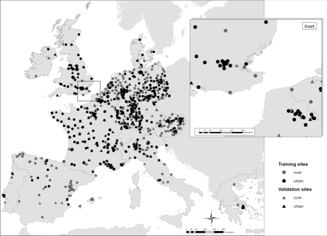
Figure 1: Locations of nitrogen dioxide monitoring sites at rural (circles) and urban (triangles) locations.

The study area comprises the EU-15 countries; Austria, Belgium, Denmark, France, Germany, Greece, Ireland, Italy, Luxembourg, The Netherlands, Portugal, Spain and the United Kingdom. However Finland and Sweden are excluded due to lack of data. Annual averages of NO₂ for 934 background monitoring sites in 2001 with $\geq$75% data capture were extracted from the Airbase database (www.eea.europa.eu/themes/air/airbase). Monitoring sites are distinguished according to site type; traffic, industrial and background and station location (urban, suburban and rural). At the time of study, these classifications were found to be incomplete and inconsistent across countries. To address this a contextually based classification, derived on the basis of discriminant analysis with consistent EU-wide land cover, was used to identify background monitoring sites. These background sites were further classified as either rural or urban (Vienneau et al., 2009). This GIS based contextual rural/urban classification also enabled classification of areas (1 km cells) across the study area, which is necessary for prediction and mapping purposes. The set of background monitoring sites were randomly allocated to either a training or validation set (comprising 75% and 25% of sites respectively), stratified by rural/urban status and country . The training and validation datasets comprise 250 rural, 458 urban and 86 rural, 140 urban sites respectively. The locations of the rural and urban training sites can be seen in Figure 1.

INSERT FIGURE 1 HERE

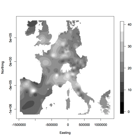
Figure 2: Smoothed plot of concentrations of NO₂ at background sites in rural locations.

A summary of the concentrations from the different locations can be seen in Table 1. As might be expected, the levels recorded at urban locations are higher than those at background locations with more variability being observed within the urban locations. Figure 2 shows the concentrations of NO₂ at the background monitoring sites located in rural areas, smoothed using multi-level B-splines Lee et al. (1997). Although these sites were chosen to ideally reflect background concentrations the effects of human activity are clearly observable particularly when rural areas are in close proximity to large cities.

INSERT TABLE 1 HERE

INSERT FIGURE 2 HERE

Covariate data were obtained from a number of sources, including CORINE (land cover), TOPO30 (topographical information), AND (transport networks), MARS (meteorology) and SIRE (population) databases and was compiled on a 1 km grid. The geographical information system (GIS) database is fully detailed in Beelen et al. (2009) and briefly summarised here. Covariates were computed at different spatial scales with the aim of representing different scales of variation: local (the immediate 1 km square within which the monitoring site lies), zonal (within the surrounding 5km neighbourhood) and regional (within the surrounding 21 km area). In each case, covariates were computed by defining a circular window around the centre of the target grid cell, and calculating the area-weighted total or average for that measure within the window. In the case of roads the value is the total length within the area and for land–use variables it is the percentage of the area attributed to that use. In the modelling it is assumed that there is a linear relationship between covariates and air pollution concentrations and so transformations were considered. For both altitude and distance to sea, the following transformation was used to address non-linear relationships; $\sqrt{x^{\prime}/max(x^{\prime})}$, where $x^{\prime}=x-min(x)$.

Here, the covariates are classified into three groups; global, rural and urban.Global level variables are those based on climate and topography and include altitude, distance to sea and meteorological variables; seasonal temperatures, wind speed, days of calm and annual radiation (9 variables). Due to the high levels of collinearity observed in these climate variables, principal component analysis was used to produce five factors, which accounted for 97% of the total variation. These five climate factors represent areas which (1) are hot year round and windy, (2) have hot summers, cooler winters, (3) are cool year round, wet and calm, (4) are cool year round, dry and calm and (5) have cold calm winters and warm windy summers. Rural and urban level covariates are based on land–use, roads and population density and are used as proxies to represent the intensity of human activities.

INSERT TABLE 2 HERE

Table 2 gives the three sets of covariates; global, rural and urban together with the scale at which they are calculated and the mean levels for rural and urban sites. Of the global variables, which will be used in both the models for rural and urban sites, it can be seen that there is little difference between rural and urban monitoring sites in terms of the climate variables and distance to sea but that the altitude of the rural sites are on average over twice that of the urban ones. Rural and urban variables are used in modelling concentrations at rural and urban sites respectively.

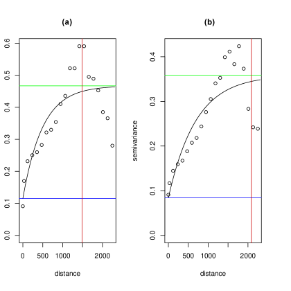
Figure 3: Variogram for (a) log values of Nitrogen Dioxide (NO₂); (b) residuals after fitting model with global and rural covariates. Lines show fitted exponential curve (black), nugget (blue), partial sill (green) and effective range at which correlation falls to 0.05 (red).

INSERT FIGURE 3 HERE

The plot of concentrations at rural locations presented in Figure 2 indicates the presence of spatial auto–correlation. Figure 3 shows the empirical variogram for measurements on the log scale from the rural sites (in the left panel) and for residuals from a multiple linear regression model using global covariates (right panel). Evidence of spatial correlation is apparent from this figure, the variogram increases from approximately 0.1 up to 0.45 corresponding to a strong correlation between close locations and then variogram levels off from 1500 km as the correlation decays to zero. The decrease of the nugget (from above 0.1 to less than 0.1) and maximum value (from ca. 4.5 to ca. 0.36) of the variogram in the right panel indicates the introduction of covariates reduces the overall spatial variation in the residuals (compared with what is essentially a model with just an intercept term). From these figures, it is suggested that there is is evidence of spatial structure in the data which should be incorporated in the model.

3 Bayesian hierarchical model

The Bayesian hierarchical model developed here has three main levels; (i) a global model which relates concentrations at rural monitoring sites to sets of global and rural covariates together with residual spatial structure, (ii) prediction using the global and spatial effects at urban locations and (iii) estimation of the effect of urban covariates using the subsequent differences in predicted and observed concentrations. In addition, a fourth level defines the hyperpriors which are required for any Bayesian analysis.

Ott (1990) has suggested that a log transformation is appropriate for modelling pollution concentrations, because in addition to the desirable properties of right-skew and non-negativity, there is justification in terms of the physical explanation of atmospheric chemistry and so the logs of the annual means at the monitoring locations are used throughout, with transformation back to the original scale for the presentation of a selection of the results.

3.1 Stage one: global level model

The aim of this stage of the model is to estimate the global effects which are then used to predict at urban locations in the next stage, allowing for the effect of the rural covariates.

Let $Y_{i}$ represent the log transformation of the annual average NO₂ concentration measured at rural sites, $i$,

$$Y_{i}=\beta_{0}+\sum^{G}_{k=1}\beta_{k}X_{i}+\sum^{p}_{k=G+1}\beta_{k}X_{i}+m_{i}+\nu_{i}$$ (1)

where $i=1,...n$. The overall mean is denoted by $\beta_{0}$ and the global and rural covariates at rural locations by the $n\times p$ matrix $X$ which is partitioned into $(X^{G},X^{R})$ denoting the G global covariates and R rural covariates. The associated regression parameters are $\beta_{1},...,\beta_{p}$. The random error terms, $\nu_{i}$, are assumed i.i.d. $N(0,\sigma^{2}_{\nu})$ with $m_{i}$. A set of spatial effects, $\mathbf{m}=(m_{1},...,m_{n})$ are assumed to arise from the multivariate normal distribution, $MVN(0_{S},\sigma^{2}_{m}\Sigma_{m})$, where $0_{S}$ is an $S\times 1$ vector of zeros, $\sigma^{2}_{m}$ the between-site variance and $\sum_{m}$ is the $S\times S$ correlation matrix. The correlation between sites is related to the distance between them and takes the form $f(d_{i,j},\phi)=\exp{(-\phi d_{i,j})}$ where $\phi>0$ describes the strength of the correlation–distance relationship, which results in a isotropic and stationary spatial model.

3.2 Stage two: prediction at urban locations

In this fully Bayesian framework, estimation of the covariate effects in the global level model and prediction at the urban locations is performed simultaneously. The uncertainty in estimating the coefficients of the global model is therefore acknowledged and ‘fed through’ the model to the predictions (this stage) and further to the estimation of the coefficients in the urban model (stage 3). However it is noted that feedback is ‘cut’ between the third and second stages (Spiegelhalter et al., 1998). It is not intended that the urban sites should inform the estimation of the global effects which should be based on data from the rural sites which are intended to provide information on background concentrations.

If the random error terms, $\nu_{j}$, in (1) are uncorrelated, then a prediction at a new location, $j$ will take the form

$$\hat{Y}_{j}=\hat{\beta}_{0}+\sum^{G}_{k=1}\hat{\beta}_{k}X_{j}+\hat{m}_{s^{{}^{\prime}}}$$ (2)

This can be viewed as two separate process; the first predicting covariate effects at new locations, using values of the global covariates at the urban locations with the values of the rural covariates which are related to human activities set to zero, and the second predicting the spatial effect. The spatial component is calculated using properties of the multivariate normal distribution. If $\mathbf{m}=(m_{1},..,m_{n})^{\prime}$ are the observed values at the monitoring locations, then the conditional distribution of $m_{j}|\mathbf{m}$ at a new location, $j$, will be normally distributed with mean and variance given by

$$E[m_{j}|\mathbf{m}]=\sigma^{-2}_{m}\mathbf{\delta}_{j}^{\prime}\Sigma^{-1}_{m}\mathbf{m},$$ (3)

and

$$var(m_{j}|\mathbf{m})=\sigma_{m}^{2}(1-\mathbf{\delta}_{j}^{\prime}\Sigma^{-1}_{m}\mathbf{\delta}_{j}),$$ (4)

respectively, where $\delta_{j}$ is the vector of distances between the new location and the monitoring sites and $\delta_{ij}=f(d_{ij},\phi)$.

3.3 Stage three: estimating urban effects

The residuals from the predictions using the global model at the urban locations are then regressed against the urban level covariates with the uncertainty from the previous stage being propagated through the model.

$$(Z_{j}-\hat{Y}_{j})=\gamma_{0}+\sum^{q}_{l=1}\gamma_{k}W_{j}+\omega_{j},$$ (5)

where $Z_{j}$ is the log transformation of the annual average measured at urban locations, $j=1,...,m$, $\gamma_{1}$ represents the overall difference between the predicted and observed levels. Urban covariates are denoted by the $m\times q$ matrix $W$ with associated regression parameters, $\gamma_{1},...,\gamma_{p}$ and $\omega_{j}$ are random error terms at urban locations which are assumed i.i.d. $N(0,\sigma^{2}_{\omega})$.

3.4 Stage four: hyperpriors

Prior distributions were assigned to all random variables, e.g. covariate effects, site effects and variances. Vague normal priors are assumed for the intercept and covariate terms, $\beta_{0},\gamma_{0},\beta_{j}$ and $\gamma_{k}\sim N(0,1000)$ with the precisions of the error terms $\nu^{-2},\omega^{-2}$ assumed to be Gamma distributed, $Ga(1,0.01)$. A uniform prior is used for the strength of the correlation–distance relationship with the limits of $\phi$ being based on beliefs about the relationship between correlation and distance. For example, the distance, $d$, at which the correlation, $\rho$, between two sites might be expected to fall to a particular level would be $d=-\log(\rho)/\phi$. Vague normal (as above) prior distributions are also assigned to the predictions at the urban locations which are in essence treated as unknown parameters with inference on the parameters of interest, i.e. the urban coefficients, being performed via averaging over the distributions of these predictions.

3.5 Inference

The joint distribution of the parameters is:

$$p(\beta,\gamma,m,\phi,\sigma^{2}_{\nu},\sigma^{2}_{\omega}\sigma^{2}_{m}|y,z) \propto p(y|\beta,m,\sigma^{2}_{\nu})$$ (6)

$$p(z|\gamma,\sigma^{2}_{\omega},\beta,m)$$

$$p(m|\phi,\sigma^{2}_{m})$$

$$p(\gamma)p(\beta)p(\sigma^{2}_{\nu})p(\phi)p(\sigma^{2}_{m})$$

which is analytically intractable but samples from this distribution may be generated in a straightforward fashion using Markov Chain Monte Carlo (MCMC) (Smith and Roberts, 1993). The prior distribution for $\beta$, $\sigma^{2}_{\nu}$ and $\sigma^{2}_{m}$ are chosen to be conjugate and Gibbs sampling can be used for all parameters, with the exception being $\phi$ which has a uniform prior and thus the full conditional is not available in closed form, requiring a Metropolis–within–Gibbs step. This was performed using the WinBUGS software (Spiegelhalter et al. (1998)).

4 Results

For each of the models presented two MCMC chains were run (for each parameter) with a minimum of 40,000 iterations as burn-in and at least a further 10,000 samples per chain used to calculate summaries of the posterior distributions. Convergence was assessed both visually and by use of the Gelman-Rubin statistic (Gelman and Rubin, 1992), which measures the ratio of the between and within chain variances. All parameters achieved convergence, although it is noted that the spatial correlation–distance parameter, $\phi$, generally took longer to converge that the other parameters.

In fitting the models vague normal priors $N(0,0.001)$ were assigned to the covariate effects and intercept terms, while for the precisions of the random error and spatial terms $Ga(1,0.01)$ were assumed. For the distance–correlation parameter, $\phi$, in the global model the limits were chosen to represent a drop to 0.01 at 25km and 2000km, i.e. representing strong and weak decays in correlation over distance respectively.

4.1 Isolating global effects

Table 3 gives the results of fitting models to data from the rural sites The most significant effect was a decrease in levels of NO₂ with increasing altitude and (in the model with both global and rural covariates) a significant positive effect was observed in relation to the fifth climate factor. When comparing a model with global level covariates with one without covariates, there is a reduction in the spatial variance, $\sigma^{2}_{m}$ indicating that much of the spatial variation in global NO₂ can be explained by the covariates, leaving less unexplained variation to be ‘mopped up’ by the spatial residual term as indicated by the variograms (Figure 3). Their inclusion also results in a reduction in the decay of correlation over distance, meaning that correlations will be greater once covariate effects have been accounted for. As an example, the correlation at 100km is 0.01 without covariates and 0.44 when they are included.

INSERT TABLE 3 HERE

The covariates also improve the model’s ability to predict at the validation locations. Calculating summary functions such as the root mean squared error (RMSE) at each iteration of MCMC simulation results in a posterior distribution as it is a simple function of other parameters being estimated. In this case, the median of the posterior distribution of the RMSE reduces from 12.9 to 9.5 when global and rural covariates are added to the model with a corresponding increase in R² from 17.5 to 44.8%. Of the 86 rural validation sites the vast majority (86%, 74/86) of the observed values lie within the 95% credible intervals for the predictions. Again this is an improvement over a model with just global covariates where the corresponding value is 58%, indicating that there is a component of levels of pollution at rural background locations which is still related to emissions from human activity which needs to be accounted for before the global effects can be examined.

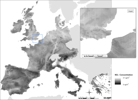
Figure 4: Predicted concentrations of NO₂ using global effects.

Figure 4 shows predicted concentrations of NO₂ throughout the EU using estimates of the global effects, i.e. based purely on their topography and climate. In comparison with Figure 2 which showed the measured concentrations, there is an overall reduction in levels of NO₂ with the effect of the urban areas close to the rural monitoring sites being markedly reduced.

INSERT FIGURE 4 HERE

4.2 Assessing the effects of human activity

The results of predicting at the urban locations using just the global and spatial effects can be seen in Figure 5. The predictions are, as expected, much lower than the observed values with the median difference being 18.7 $\mu gm^{-3}$ (IQR, 13.1 - 25.4) and this difference will be examined in relation to urban factors.

INSERT FIGURE 5 HERE

Table 4 gives the results of fitting models to data from the urban sites, where differences between observed urban NO₂ concentration and that predicted as though they were background locations are explained by the effects of urban covariates. In a model without covariates the intercept term, representing the urban increment, is 3.294 representing an (significant) overall increase of 27 $\mu$g$m^{-3}$. In the model including urban covariates, there is again a positive (significant) urban intercept term with all the urban level covariates show further positive associations with levels of NO₂, except for urban greenery. Major roads has the largest significant effect with an relative increase of 1.06 $\mu$gm^-3 (=exp(0.0623)) associated with an increase of 1 km of road length (in the surrounding 1 km area) with high density residential also having a significant association.

INSERT TABLE 4 HERE

5 Discussion

In this paper we consider air pollution as a multi–level phenomenon within a Bayesian hierarchical model. Different scales of variation are considered ranging from large scale transboundary effects to more localised effects which are related to human activity. The aim of the first stage of the model is to isolate underlying patterns in pollution concentrations due to global factors, such as underlying climate and topography, from those arising from land use and traffic. At this stage monitoring sites located within rural areas were used which, as much as is possible, were chosen to reflect background concentrations. However, in all but the most remote of areas there will still be some effect of human activity on levels of pollution and so carefully selected covariates representing emission sources, such as land cover or road density, were used at either zonal or regional levels (representing the surrounding 5km and 21km respectively) to isolate global effects together with long-range spatial structure.

Having isolated these effects, in the second stage of the model we assess the effects of human activity on levels of pollution in urban areas where such activity will be greatest. We found a significant increase in levels of NO₂ in urban areas compared to that which might be expected based on global effects alone. The estimated increase from the second stage of the model was 27.0 $\mu$gm^-3 (95% CI 26.1 – 27.9) which is considerably greater than the difference observed between the means of the concentrations observed at rural and urban sites (13 $\mu$gm^-3). This is because the concentrations observed at the majority of rural locations will inevitably include some component which is due to human activity in the surrounding area. They therefore cannot be assumed to give a true reflection of background concentrations without accounting for the resulting emissions as we have attempted to do here in the first stage of the model.

We assume that pollution varies smoothly on a global scale and that urban areas are embedded in an overall spatial surface. Here, this global spatial structure in the first stage of the model is assumed to be isotropic and stationary. The assumption of isotropy can to some extent be assessed by constructing variograms in different directions, which in this case showed little evidence of ansitropy (not shown). The assumption of stationarity might be tenable for the global scale, after adjustment for covariate effects, whereas using a such a model to address finer scale variation over a large number of urban areas might be less reasonable. The ability of a spatial model to provide accurate predictions can to some extent be assessed by validation, but there may be underlying problems based on the availability of data over the entire study area. For example, (i) the covariates may not fully reflect the areas in which the pollution is measured, i.e. other important covariates may have been excluded or are not available; (ii) the spatial structure in the model is sufficiently flexible to be able to accurately reflect complexity of air pollution process and (iii) the location of monitoring sites may not fully represent the spatial pattern of pollution over the study region, i.e. the monitoring sites are unevenly distributed over the region and are not able to represent the underlying spatial process.

The approach used here is similar in concept to the two step regression modelling strategy of Beelen et al. (2009), although the specific aim of that paper was to perform mapping. Their two step procedure involved fitting two separate models and using the prediction from the first as a fixed covariate for the second, thus ignoring the fact that the prediction is an estimate based on the first regression and is thus subject to uncertainty. By performing both models simultaneously within a Bayesian hierarchical framework, this uncertainty is acknowledged and correctly ‘fed through’ the model. We performed a comparative analysis using a two-stage approach in which uncertainty was not fed though the model and found the confidence intervals were much narrower. For example, in the case of the estimate of the effect of major roads the width of the credible interval reduced from 0.115 to 0.056 (data not shown).

An alternative approach would have been to combine the rural and urban sites in a single model, however that would lead to high–levels of collinearity between measurements at different scales, or to fit global and urban effects together using data from urban locations. However, the influence of human activity on concentrations of pollution in urban locations is so strong that, even after covariate adjustment, they cannot be used to represent background levels. In practice, this means that the urban covariates are likely to dominate the global ones to such an extent that interpreting the global part of the model would be very difficult. In performing such an analysis we found, for example, that the effect of altitude was positive which is entirely counter intuitive for NO₂. In contrast, the approach used in this paper allows us to combine data from both rural and urban sites, to estimate background concentrations and therefore quantify the contribution to air pollution attributable to human activity within a coherent modelling framework.

The models proposed here provide valuable information that could be used in performing health impact assessments and to inform policy. For example, further research could utilise the the differences in urban and background concentrations in order to assess the health risk of air pollution that is attributable to human activity.

Table 1: Summary of NO₂ concentrations by site location; annual means for 2001

Location	Mean	SD	Median	IQR	Min-Max
All	24	12	23	(16-31)	2-74
Rural	16	9	14	(9-21)	2-43
Urban	29	10	27	(21-35)	8-74

Table 2: Summary (means) of covariates at locations of NO₂ monitoring sites (training set) at all, rural and urban locations. See text for descriptions of the covariates and the resolution at which they are computed.

Covariate	All sites	Backgound	Urban
Global
Altitude (m)	220	360	145
Distance to sea (m)	202	198	205
Climate factor 1	0.83	0.71	0.90
Climate factor 2	-0.42	-0.20	-0.55
Climate factor 3	0.25	0.26	0.24
Climate factor 4	0.05	-0.02	0.08
Climate factor 5	-0.03	-0.03	-0.03
Rural
Major roads (5 km)	10.85	0.65	14.64
Minor roads (5 km)	35.59	2.42	42.70
High density residential (5 km)	5.74	0.57	8.56
Low density residential (5 km)	26.14	6.05	37.10
Agriculture (5 km)	45.95	50.5	44.60
Non-rural built up (21 km)	3.72	1.30	5.04
Forestry (21 km)	19.84	27.05	15.90
Urban
Major roads (1km)	0.65	0.25	0.87
Minor roads (1km)	2.42	1.32	3.02
High density residential (1 km)	11.00	0.64	16.70
Low density residential (1 km)	38.8	7.54	55.9
Industry (1 km)	6.12	1.08	8.86
Transport (1 km)	0.93	0.05	1.41
Sea port (1 km)	0.30	0.03	0.48
Air port (1 km)	0.20	0.07	0.45
Construction (1 km)	0.56	0.36	0.67
Urban Greenery (1 km)	2.24	0.18	3.36

Table 3: Rural monitoring sites: Summaries of posterior distributions of parameters; medians and 95% credible intervals for models with and without covariates. Models are fit with (i) intercept term, (ii) global covariates and (iii) global and rural covariates.

	(i)			(ii)			(iii)
	Median	$2.5\%$	$97.5\%$	Median	$2.5\%$	$97.5\%$	Median	$2.5\%$	$97.5\%$
Intercept	2.5830	2.4660	3.1790	3.2110	2.6640	3.8160	2.4150	1.8440	3.1000
Altitude				-3.5580	-4.3720	-2.8000	-1.9970	-2.9720	-1.0870
Dist. sea				0.6367	-0.1733	1.3480	0.2754	-0.4621	0.8936
Climate factor 1				-0.1725	-0.3591	-0.0147	-0.1159	-0.2991	0.0283
Climate factor 2				0.0296	-0.0933	0.1023	0.0140	-0.0664	0.0771
Climate factor 3				-0.0930	-0.2523	0.0850	-0.0475	-0.2309	0.0942
Climate factor 4				-0.1839	-0.3424	-0.0294	-0.1213	-0.2744	0.0185
Climate factor 5				0.3096	-0.0190	0.6182	0.2880	0.0090	0.5467
Major road							0.0181	0.0031	0.0329
Minor road							0.0082	0.0012	0.0153
High density res.							0.1925	0.0221	0.3666
Low density res.							0.0070	-0.0024	0.0164
Agriculture							0.0039	0.0009	0.0069
Non-rural built up							0.0383	0.0071	0.0690
Forestry							0.0005	-0.0044	0.0054
$\phi$	0.0437	0.0284	0.0726	0.0075	0.0029	0.0252	0.0106	0.0030	0.1431
$\sigma_{m}$	0.6382	0.5760	0.7062	0.5057	0.3739	0.7265	0.4108	0.2859	0.5366

Table 4: Model for examining human activity on NO₂ concentration: the difference between concentrations measured at urban locations and predictions based on global variables. Models are fit with (i) intercept term, (ii) urban covariates.

	(i)			(ii)
	Median	$2.5\%$	$97.5\%$	Median	$2.5\%$	$97.5\%$
Intercept (urban)	3.2940	3.2630	3.3270	0.8369	0.4291	1.2570
Major road				0.0623	0.0036	0.1186
Minor road				0.0266	-0.0171	0.0653
High density residential				0.0041	0.0003	0.0088
Low density residential				0.0013	-0.0025	0.0051
Industrial				0.0016	-0.0029	0.0064
Transport				0.0069	-0.0031	0.0173
Sea port				0.0072	-0.0129	0.0245
Air port				0.0001	-0.0135	0.0154
Construction				0.0058	-0.0044	0.0154
Urban greenery				-0.0022	-0.0115	0.0058

Figure 5: Comparison of the observed concentrations at the urban locations with predictions from model using only global effects. Left hand panel (a) shows plot of predicted versus observed concentrations, right hand panel (b) shows a histogram of the differences.

References

- Abbey et al. (1999) Abbey, D., N. Nishino, W. McDonnel, and et al. (1999). Long-term inhalable particles and other air pollutants related to mortality in nonsmokers. Am. J. Respir. Crit. Care Med. 159, 373–82.
- Anderson (1967) Anderson, D. (1967). The effects of air contamination on health. I. Canadian Medical Association Journal 97(10), 528.
- Anderson (2009) Anderson, H. (2009). Air pollution and mortality: A history. Atmospheric Environment 43(1), 142–152.
- Ayres et al. (1972) Ayres, S., R. Evans, and M. Buehler (1972). Air pollution: A major public health problem. Critical Reviews in Clinical Laboratory Sciences 3(1), 1–40.
- Beelen et al. (2009) Beelen, R., G. Hoek, E. Pebesma, D. Vienneau, K. de Hoogh, and D. Briggs (2009). Mapping of background air pollution at a fine spatial scale across the European Union. Science of the Total Environment 407(6), 1852–1867.
- Briggs (2005) Briggs, D. (2005). The role of GIS: coping with space (and time) in air pollution exposure assessment. Journal of Toxicology and Environmental Health, Part A 68(13), 1243–1261.
- Briggs et al. (1997) Briggs, D., S. Collins, P. Elliott, P. Fischer, S. Kingham, E. Lebret, K. Pryl, H. Van Reeuwijk, K. Smallbone, and A. Van Der Veen (1997). Mapping urban air pollution using GIS: a regression-based approach. International Journal of Geographical Information Science 11(7), 699–718.
- Briggs et al. (2000) Briggs, D., C. de Hoogh, J. Gulliver, J. Wills, P. Elliott, S. Kingham, and K. Smallbone (2000). A regression-based method for mapping traffic-related air pollution: application and testing in four contrasting urban environments. The science of the total environment 253(1-3), 151–167.
- Brimblecombe (1987) Brimblecombe, P. (1987). The big smoke: a history of air pollution in London since medieval times. Routledge Kegan & Paul.
- Brunekreef and Holgate (2002) Brunekreef, B. and S. Holgate (2002). Air pollution and health. The Lancet 360(9341), 1233–1242.
- Carr et al. (2002) Carr, D., O. von Ehrenstein, S. Weiland, C. Wagner, O. Wellie, T. Nicolai, and E. von Mutius (2002). Modeling annual benzene, toluene, NO2, and soot concentrations on the basis of road traffic characteristics. Environmental research 90(2), 111–118.
- Chew et al. (1999) Chew, F., D. Goh, B. Ooi, R. Saharom, J. Hui, and B. Lee (1999). Association of ambient air-pollution levels with acute asthma exacerbation among children in Singapore. Allergy 54(4), 320–329.
- Dominici et al. (2002) Dominici, F., M. Daniels, S. Zeger, and J. Samet (2002). Air pollution and mortality. Journal of the American Statistical Association 97(457), 100–111.
- Elliott et al. (2007) Elliott, P., G. Shaddick, J. Wakefield, C. Hoogh, and D. Briggs (2007). Long-term associations of outdoor air pollution with mortality in Great Britain. Thorax 62(12), 1088.
- Finkelstein et al. (2003) Finkelstein, M., M. Jerrett, P. Deluca, and et al. (2003). Relation between income, air pollution and mortality: a cohort study. CMAJ. 169, 397–402.
- Garner and Crow (1969) Garner, J. and R. Crow (1969). Clean Air-Law and Practice. Shaw and Sons Ltd.
- Gelman and Rubin (1992) Gelman, A. and D. Rubin (1992). Inference from iterative simulation using multiple sequences. Statistical science 7(4), 457–472.
- Gilbert et al. (2005) Gilbert, N., M. Goldberg, B. Beckerman, J. Brook, and M. Jerretft (2005). Assessing spatial variability of ambient nitrogen dioxide in Montreal, Canada, with a land-use regression model. Journal of the Air & Waste Management Association 55(8), 1059–1063.
- Giussani et al. (1994) Giussani, V., C. for Social, and E. R. on the Global Environment (1994). The UK clean air act 1956: an empirical investigation. CSERGE Norwich.
- Heimann (1961) Heimann, H. (1961). Effects of air pollution on human health. Air pollution, 159–220.
- Henderson et al. (2007) Henderson, S., B. Beckerman, M. Jerrett, and M. Brauer (2007). Application of land use regression to estimate long-term concentrations of traffic-related nitrogen oxides and fine particulate matter. Environ. Sci. Technol 41(7), 2422–2428.
- Hoek et al. (2008) Hoek, G., R. Beelen, K. de Hoogh, D. Vienneau, J. Gulliver, P. Fischer, and D. Briggs (2008). A review of land-use regression models to assess spatial variation of outdoor air pollution. Atmospheric environment 42(33), 7561–7578.
- Hoek et al. (2002) Hoek, G., B. Brunekreef, S. Goldbohm, and et al. (2002). Association between mortality and indicators of traffic-related air pollution in the Netherlands: a cohort study. Lancet. 360, 1203–9.
- Jerrett et al. (2005) Jerrett, M., R. Burnett, R. Ma, and et al. (2005). Spatial analysis of air pollution and mortality in Los Angeles. Epidemiology. 16, 727–36.
- Katsouyanni et al. (2001) Katsouyanni, K., G. Touloumi, E. Samoli, A. Gryparis, A. Le Tertre, Y. Monopolis, G. Rossi, D. Zmirou, F. Ballester, A. Boumghar, et al. (2001). Confounding and effect modification in the short-term effects of ambient particles on total mortality: results from 29 European cities within the APHEA2 project. Epidemiology 12(5), 521.
- Katsouyanni et al. (1997) Katsouyanni, K., G. Touloumi, C. Spix, J. Schwartz, F. Balducci, S. Medina, G. Rossi, B. Wojtyniak, J. Sunyer, L. Bacharova, et al. (1997). Short term effects of ambient sulphur dioxide and particulate matter on mortality in 12 European cities: results from time series data from the APHEA project. British Medical Journal 314(7095), 1658.
- Lee et al. (1997) Lee, S., G. Wolberg, and S. Shin (1997). Scattered data interpolation with multilevel b-splines. Visualization and Computer Graphics, IEEE Transactions on 3(3), 228–244.
- Madsen et al. (2007) Madsen, C., K. Carlsen, G. Hoek, B. Oftedal, P. Nafstad, K. Meliefste, R. Jacobsen, W. Nystad, K. Carlsen, and B. Brunekreef (2007). Modeling the intra-urban variability of outdoor traffic pollution in Oslo, Norway–A GA2LEN project. Atmospheric Environment 41(35), 7500–7511.
- Nafstad et al. (2003) Nafstad, P., L. Haheim, B. Oftedal, F. Gram, I. Holme, I. Hjermann, and P. Leren (2003). Lung cancer and air pollution: a 27 year follow up of 16209 Norwegian men. Thorax 58(12), 1071.
- Ott (1990) Ott, W. (1990). A Physical Explanation of the Lognormality of Pollutant Concentrations. Journal of the Air Waste Management Association 40, 1378–1383.
- Pope et al. (1995) Pope, C., D. Dockery, and J. Schwartz (1995). Review of epidemiological evidence of health effects of particulate air pollution. Inhalation Toxicology 7(1), 1–18.
- Rosenlund et al. (2006) Rosenlund, M., N. Berglind, G. Pershagen, and et al. (2006). Long-term exposure to urban air pollution and myocardial infarction. Epidemiology 17, 383–90.
- Ross et al. (2005) Ross, Z., P. English, R. Scalf, R. Gunier, S. Smorodinsky, S. Wall, and M. Jerrett (2005). Nitrogen dioxide prediction in Southern California using land use regression modeling: potential for environmental health analyses. Journal of Exposure Science and Environmental Epidemiology 16(2), 106–114.
- Smith and Roberts (1993) Smith, A. and G. Roberts (1993). Bayesian computation via the Gibbs sampler and other related Markov chain Monte Carlo methods. Journal of the Royal Statistical Society series B 55, 3–23.
- Snyder (1994) Snyder, L. (1994). The Death-Dealing Smog over Donora, Pennsylvania”: Industrial Air Pollution, Public Health Policy, and the Politics of Expertise, 1948-1949. Environmental History Review 18(1), 117–139.
- Spiegelhalter et al. (1998) Spiegelhalter, D., A. Thomas, and N. Best (1998). WinBUGS user manual, version 1.1. 1. Cambridge, UK.
- Stern et al. (1973) Stern, A., H. Wohlers, R. Boubel, and W. Lowry (1973). Fundamentals of Air Pollution. Academic Press.
- Stone (2002) Stone, R. (2002). AIR POLLUTION: Counting the Cost of London’s Killer Smog. Science 298(5601), 2106.
- Vienneau et al. (2009) Vienneau, D., K. De Hoogh, and D. Briggs (2009). A gis-based method for modelling air pollution exposures across europe. Science of the Total Environment 408(2), 255–266.
- WHO (2005) WHO (2005). Air quality guidelines: Global update 2005. World Health Organization, Bonn, Germany.