TTK-11-51
SFB/CPP-11-56
October 14, 2011

$B$ meson distribution amplitude from $B\to\gamma\ell\nu$

M. Beneke and J. Rohrwild

Institut für Theoretische Teilchenphysik und Kosmologie,
RWTH Aachen University,
D-52074 Aachen, Germany

Abstract
We reconsider the utility of the radiative decay $B\to\gamma\ell\nu$ with an energetic photon in the final state for determining parameters of the $B$-meson light-cone distribution amplitude. Including $1/m_{b}$ power corrections and radiative corrections at next-to-leading logarithmic order, we perform an improved analysis of the existing BABAR data. We find a provisional lower limit on the inverse moment of the $B$ meson distribution amplitude, $\lambda_{B}$, which, due to the inclusion of radiative and power corrections, is significantly lower than the previous result. More data with large photon energy is, however, required to obtain reliable results, as should become available in the future from SuperB factories.

1 Introduction

The decay of the charged $B$ meson into a photon, lepton and neutrino is sometimes perceived as an unwanted background to the purely leptonic decay process $B^{-}\to\ell\bar{\nu}$ [1], which allows for a determination of $V_{ub}$. Still, the radiative leptonic decay is of interest in itself for the theory of heavy meson decays, especially when the energy $E_{\gamma}$ of the photon is of order of the bottom quark mass, $m_{b}$. Its factorization properties have been studied at leading order in the heavy-quark expansion [2, 3, 4, 5] and it has been shown that the decay amplitude can be calculated in terms of the inverse and inverse-logarithmic moments of the $B$-meson light-cone distribution amplitude [7, 6, 8].

The branching fraction of the radiative decay depends very strongly on the inverse moment $\lambda_{B}$, where $1/\lambda_{B}=\int_{0}^{\infty}\!{\rm d}\omega\,\Phi_{B+}(\omega)/\omega$. It therefore seems very well suited as an observable to measure $\lambda_{B}$, which is an important parameter in the QCD factorization approach to non-leptonic $B$ decays [7], but is very difficult to obtain reliably by theoretical methods, the most advanced being QCD sum rules [9]. We are aware of only two analyses by the BABAR collaboration that set limits on the $B^{-}\to\gamma\ell\bar{\nu}$ branching fraction and $\lambda_{B}$ [10, 11]. The first reports $\lambda_{B}>669\,\mbox{MeV}\,(591\,\mbox{MeV})$ (depending on the treatment of priors), while the second, published analysis concludes the significantly weaker limit $\lambda_{B}>300\,\mbox{MeV}$. The first result would be rather troublesome for non-leptonic $B$ decay phenomenology, which needs $\lambda_{B}\approx 200\,\mbox{MeV}$ to achieve a satisfactory description of color-suppressed decay modes [12, 13, 14].

The BABAR analyses should be taken with a grain of salt, since, presumably in order not to sacrifice statistics, they do not require the photons to be sufficiently energetic for the theoretical calculation to be valid. This can certainly be improved in the future, in particular with the high statistics foreseen at the SuperB experiments. They also do not include radiative corrections, which is one of our concerns in this note. We show that after including next-to-leading logarithmically resummed corrections, and after correcting an error in the literature in the leading $1/m_{b}$ correction, the predicted branching fraction is significantly smaller. This reduces the lower limit on $\lambda_{B}$ considerably.

The outline this paper is as follows. In Sec. 2 and the Appendix we briefly review the theoretical background and summarize the expression for the $B\to\gamma\ell\nu$ amplitude. Sec. 3 discusses the size and stability of radiative corrections and the $B\to\gamma$ form factors themselves. In Sec. 4 we repeat the BABAR analysis in order to demonstrate the impact of our results on the bound on $\lambda_{B}$. We conclude in Section 5.

2 Theory summary of $B\to\gamma\ell\nu$ decay

We consider the decay of a $B$ meson with mass $m_{B}$ and momentum $p^{\mu}=m_{B}v^{\mu}$ into a photon with momentum $q$, a neutrino with momentum $p_{\nu}$ and a lepton (momentum $p_{\ell}$). The lepton and neutrino are assumed to be massless, which restricts us to $\ell=e,\mu$. In the $B$ meson rest frame the photon energy satisfies $E_{\gamma}\leq m_{B}/2$. We introduce the abbreviations $x_{i}=\frac{2E_{i}}{m_{B}}$ where $i$ can be either $\gamma$, $\ell$ or $\nu$. We have $0\leq x_{i}\leq 1$ and $x_{\gamma}+x_{\ell}+x_{\nu}=2$. The amplitude for the decay $B\to\gamma\ell\nu$ can be written as

$$\mathcal{A}(B^{-}\to\gamma\ell\bar{\nu})=\frac{G_{F}V_{ub}}{\sqrt{2}}\,\langle{\ell\bar{\nu}\gamma}|\bar{\ell}\gamma^{\mu}(1-\gamma_{5})\nu\cdot\overline{u}\gamma^{\mu}(1-\gamma_{5})b|{B^{-}}\rangle\;.$$ (2.1)

The photon can be emitted either from the final-state lepton or from one of the constituents of the $B$ meson. This can be made explicit by rewriting the matrix element using the electromagnetic current $j^{\mu}_{\rm em}=\sum_{q}Q_{q}\overline{q}\gamma_{\mu}q+Q_{\ell}\bar{\ell}\gamma_{\mu}\ell$. To first order in electromagnetic and to all orders in the strong interaction, we have

$$\langle{\ell\bar{\nu}\gamma}|\overline{\ell}\gamma^{\mu}(1-\gamma_{5})\nu\cdot\overline{u}\gamma_{\mu}(1-\gamma_{5})b|{B^{-}}\rangle=$$

$$\hskip 28.45274pt=-ie\epsilon^{\star}_{\nu}\left[\langle{\ell\bar{\nu}}|\bar{\ell}\gamma^{\mu}(1-\gamma_{5})\nu)|{0}\rangle\cdot\int\!{\rm d}^{4}x\,e^{iqx}\langle{0}|{\rm T}\{j_{\rm em}^{\nu}(x)(\overline{u}\gamma_{\mu}(1-\gamma_{5})b)(0)\}|{B^{-}}\rangle\right.\qquad$$

$$\hskip 28.45274pt\left.\qquad\qquad+\int\!{\rm d}^{4}x\,e^{iqx}\langle{\ell\bar{\nu}}|{\rm T}\{j_{\rm em}^{\nu}(x)(\bar{\ell}\gamma^{\mu}(1-\gamma_{5})\nu)(0)\}|{0}\rangle\cdot\langle{0}|\overline{u}\gamma_{\mu}(1-\gamma_{5})b|{B^{-}}\rangle\right]$$

$$\hskip 28.45274pt=e\epsilon^{\star}_{\nu}\,\bar{u}_{\ell}\gamma_{\mu}(1-\gamma_{5})u_{\nu}\cdot T^{\nu\mu}(p,q)-ieQ_{\ell}f_{B}\cdot\bar{u}_{\ell}\not{\epsilon}^{\star}(1-\gamma_{5})u_{\nu}\,.$$ (2.2)

Note that we use $iD^{\mu}=i\partial^{\mu}-Q_{\psi}eA^{\mu}_{em}$ for the QED covariant derivative with $e$ the charge of the positron, and $Q_{\psi}$ the electric charge of fermion $\psi$ in units of $e$. The first term in the above equation corresponds to the emission from the meson constituents whereas the second term describes the emission from the lepton, and can be calculated exactly using

$$\langle{0}|\overline{u}\gamma^{\mu}(1-\gamma_{5})b|{B^{-}(p)}\rangle=-if_{B}p^{\mu}\,.$$ (2.3)

The hadronic tensor can be parameterized as

$$T_{\nu\mu}(p,q) = (-i)\int\!{\rm d}^{4}x\,e^{iqx}\langle{0}|{\rm T}\{j_{\nu,\rm em}(x)(\overline{u}\gamma_{\mu}(1-\gamma_{5})b)(0)\}|{B^{-}}\rangle$$ (2.4)

$$=\,(-i)\left[i\epsilon_{\mu\nu\rho\sigma}v^{\rho}q^{\sigma}\,F_{V}(E_{\gamma})+(g_{\mu\nu}v\cdot q-v_{\nu}q_{\mu})\,\hat{F}_{A}(E_{\gamma})+\frac{v_{\nu}v_{\mu}}{v\cdot q}\,f_{B}m_{B}+q_{\nu}\mbox{-terms}\right].\qquad$$

The terms proportional to $q_{\nu}$ are irrelevant, since $\epsilon^{\star}\cdot q=0$. The $v_{\nu}v_{\mu}$ structure is often referred to as “contact term”. Its coefficient is fixed by the electromagnetic current conservation Ward identity $q_{\nu}T^{\nu\mu}=-if_{B}p^{\mu}$ [15]. The remainder consists of two form factors. In the following we shall describe the QCD calculation of these form factors for photon energies of order (but not necessarily near) $m_{B}/2$.

With the help of $(p-q)^{\mu}\,\bar{u}_{\ell}\gamma_{\mu}(1-\gamma_{5})u_{\nu}=0$, valid for massless leptons, we may replace

$$(g_{\mu\nu}v\cdot q-v_{\nu}q_{\mu})\,\hat{F}_{A}(E_{\gamma})+\frac{v_{\nu}v_{\mu}}{v\cdot q}\,f_{B}m_{B}\to(g_{\mu\nu}v\cdot q-v_{\nu}q_{\mu})\,F_{A}(E_{\gamma})+g_{\mu\nu}f_{B}$$ (2.5)

in (2.4), where the new axial form factor is defined as

$$F_{A}=\hat{F}_{A}+\frac{Q_{\ell}f_{B}}{E_{\gamma}}\,.$$ (2.6)

In this form the $g_{\mu\nu}f_{B}$ term in (2.5) cancels precisely the last term in (2.2) from photon emission off the lepton, and the amplitude (2.1) is expressed entirely in terms of the two form factors $F_{V,A}$. We use this convention below. However, the decomposition (2.4) is useful for calculations, since it allows us to assume that the indices $\mu,\nu$ are transverse relative to the four-vectors $v$ and $q$, such that $F_{V}$ and $\hat{F}_{A}$ can be extracted from the $\epsilon_{\mu\nu\rho\sigma}$ and $g_{\mu\nu}$ structures of the hadronic tensor, respectively.

Squaring the amplitude, the doubly differential decay width in the $B$ rest frame reads

$$\frac{\!{\rm d}^{2}\Gamma}{\!{\rm d}E_{\gamma}\,\!{\rm d}E_{\ell}}=\frac{\alpha_{\rm em}G_{F}^{2}|V_{ub}|^{2}}{16\pi^{2}}m_{B}^{3}(1-x_{\gamma})\left[(1-x_{\nu})^{2}(F_{A}+F_{V})^{2}+(1-x_{\ell})^{2}(F_{A}-F_{V})^{2}\right],$$ (2.7)

where $E_{\ell}+E_{\gamma}\geq m_{B}/2$, and the form factors depend on $E_{\gamma}$ but not on the lepton energy $E_{\ell}$. Further integration results in

$$\frac{\!{\rm d}\Gamma}{\!{\rm d}E_{\gamma}}=\frac{\alpha_{\rm em}G_{F}^{2}|V_{ub}|^{2}}{48\pi^{2}}m_{B}^{4}(1-x_{\gamma})x_{\gamma}^{3}\left[F_{A}^{2}+F_{V}^{2}\right].$$ (2.8)

For energetic photons, the form factors are given by

$$F_{V}(E_{\gamma}) = \frac{Q_{u}m_{B}f_{B}}{2E_{\gamma}\lambda_{B}(\mu)}\,R(E_{\gamma},\mu)+\left[\xi(E_{\gamma})+\frac{Q_{b}m_{B}f_{B}}{2E_{\gamma}m_{b}}+\frac{Q_{u}m_{B}f_{B}}{(2E_{\gamma})^{2}}\right],$$

$$F_{A}(E_{\gamma}) = \frac{Q_{u}m_{B}f_{B}}{2E_{\gamma}\lambda_{B}(\mu)}\,R(E_{\gamma},\mu)+\left[\xi(E_{\gamma})-\frac{Q_{b}m_{B}f_{B}}{2E_{\gamma}m_{b}}-\frac{Q_{u}m_{B}f_{B}}{(2E_{\gamma})^{2}}+\frac{Q_{\ell}f_{B}}{E_{\gamma}}\right].\quad$$ (2.9)

The first term represents the leading-power contribution in the heavy-quark expansion with $R(E_{\gamma},\mu)$ a radiative correction factor that equals one at tree level. Note that this term is the same for the vector and axial form factor [2, 3, 4, 5]. The terms in square brackets are $1/m_{b}$ power corrections relative to the leading term. They consist of a term $\xi(E_{\gamma})$ that is common to both form factors (“symmetry-preserving”) and other terms of a simple form that differ (“symmetry-breaking”). We do not include perturbative radiative corrections to the power-suppressed terms.

We note that $(F_{V}-F_{A})/(F_{V}+F_{A})\sim\Lambda_{\rm QCD}/m_{b}$ is suppressed in the heavy-quark limit due to helicity conservation. The second term proportional to $(1-x_{\ell})^{2}$ in (2.7) is therefore suppressed.

Radiative corrections

Radiative corrections to the $B^{-}\to\gamma\ell\bar{\nu}$ process were first calculated in a $k_{t}$-dependent approach [2]; see [16] for an extended analysis of the decay in this approach. However, there is no need not to integrate over $k_{t}$. The all-order factorization formula [4, 5] refers to this situation. The one-loop radiative corrections in collinear factorization have been computed some time ago [3, 4, 5] and we summarize them here. Our improvement consists in completing the next-to-leading logarithmic (NLL) summation of logarithms of $m_{b}/\Lambda_{\rm QCD}$, since the two-loop anomalous dimension of the heavy-light current is now known.

The radiative correction can be written as a product of several factors,

$$R(E_{\gamma},\mu)=C(E_{\gamma},\mu_{h1})K^{-1}(\mu_{h2})\times U(E_{\gamma},\mu_{h1},\mu_{h2},\mu)\times J(E_{\gamma},\mu),$$ (2.10)

which come from the different scales contributing to the process. The multiplicative structure becomes transparent if the decay is analyzed in soft-collinear effective theory (SCET) [21, 22, 23, 24] as done in [4, 5]. The first factor arises from the hard scale $m_{b}$ when the QCD heavy-to-light current is matched to the corresponding SCET current:

$$\overline{u}\gamma_{\mu_{\perp}}(1-\gamma_{5})b=C(E_{\gamma},\mu)\,\bar{\xi}W_{c}\gamma_{\mu_{\perp}}(1-\gamma_{5})h_{v}+\ldots$$ (2.11)

with [21]

$$C(E_{\gamma},\mu)=1+\frac{\alpha_{s}C_{F}}{4\pi}\left(-2\ln^{2}\frac{2E_{\gamma}}{\mu}+5\ln\frac{2E_{\gamma}}{\mu}-\frac{3-2x}{1-x}\ln x-2{\rm Li}_{2}(1-x)-6-\frac{\pi^{2}}{12}\right)$$ (2.12)

and $x=2E_{\gamma}/m_{b}$. The two-loop correction is also known [17, 18, 19, 20], but at NLL accuracy we only need the one-loop term and two-loop anomalous dimension of the SCET current, which can be inferred from [17, 18, 19, 20]. After inserting (2.11) into (2.4), the hadronic tensor factorizes into a hard-collinear contribution from the scale $(m_{b}\Lambda_{\rm QCD})^{1/2}$ and moments of the non-perturbative light-cone distribution amplitude (LCDA) of the $B$ meson. We define these moments as

$$\frac{1}{\lambda_{B}(\mu)}=\int_{0}^{\infty}\frac{\!{\rm d}\omega}{\omega}\,\Phi_{B+}(\omega,\mu),\qquad\sigma_{n}(\mu)=\lambda_{B}(\mu)\int_{0}^{\infty}\frac{\!{\rm d}\omega}{\omega}\,\ln^{n}\frac{\mu_{0}}{\omega}\,\Phi_{B+}(\omega,\mu)$$ (2.13)

where $\mu_{0}=1\,\mbox{GeV}$ is a fixed reference scale which is part of the definition of the inverse-logarithmic moments. The hard-collinear radiative correction reads [4, 5]

$$J(E_{\gamma},\mu)=1+\frac{\alpha_{s}C_{F}}{4\pi}\left(\ln^{2}\frac{2E_{\gamma}\mu_{0}}{\mu^{2}}-2\sigma_{1}(\mu)\ln\frac{2E_{\gamma}\mu_{0}}{\mu^{2}}-1-\frac{\pi^{2}}{6}+\sigma_{2}(\mu)\right).$$ (2.14)

Since the SCET current in (2.11) uses the static heavy-quark field $h_{v}$, we encounter the static $B$ meson decay constant when taking the matrix element. We re-express this in terms of the QCD decay constant $f_{B}$, which introduces the conversion factor

$$K(\mu)=1+\frac{\alpha_{s}C_{F}}{4\pi}\left(\frac{3}{2}\ln\frac{m_{b}^{2}}{\mu^{2}}-2\right).$$ (2.15)

Inspecting (2.12), (2.14) and (2.15) shows that there is no common value of $\mu$ that avoids parametrically large logarithms of order $\ln m_{b}/\mu_{0}$. These logarithms can be summed to all orders by solving a renormalization group equation [5], which introduces the evolution factor $U(E_{\gamma},\mu_{h1},\mu_{h2},\mu)$ into (2.10). Its explicit expression is given in the appendix. The hard scales $\mu_{h1},\mu_{h2}$ can (and should) now be taken ${\cal O}(m_{b})$, the hard-collinear scale $\mu\sim{\cal O}(m_{b}\Lambda_{\rm QCD})^{1/2}$. Eqs. (2.12) and (2.15) suggest that the hard scale $\mu_{h1}$ is $2E_{\gamma}$ rather than $m_{b}$, while $\mu_{h2}\sim m_{b}$, which motivates keeping the two hard scales distinct in the general expressions. However, we might also set them equal, which is the conventional procedure.

Power corrections

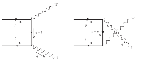
Figure 1: Leading-order diagrams. The left graph shows the leading-power contribution from photon emission from the up anti-quark. Emission from the heavy $b$-quark (right) is power suppressed.

For phenomenology $1/m_{b}$ corrections are presumably important. Power corrections are notoriously difficult for factorization approaches, but $B\to\gamma\ell\nu$ is arguably the simplest environment to study them. Here we explain the origin of the “tree-level” $1/m_{b}$-suppressed terms in (2.9), which are the most relevant to phenomenology, and defer the general discussion of $1/m_{b}$ power corrections to future work [26].

The two diagrams for the tree-level $b\bar{u}\to\gamma W^{*}$ amplitude are shown in Fig. 1. Since the spectator-quark momentum $l\sim\Lambda_{\rm QCD}$ is soft, the propagator joining the $W$ and $\gamma$ lines has hard-collinear virtuality $(q-l)^{2}=2q\cdot l\sim m_{b}\Lambda_{\rm QCD}$, when the photon is emitted from the up anti-quark (left), but hard virtuality $(p-q)^{2}\sim m_{b}^{2}$ in case of emission from the heavy quark (right). For this reason only emission from the light anti-quark is responsible for the leading-power contribution in (2.9). The emission from the heavy quark can easily by calculated and results in the power-suppressed term proportional to the bottom-quark charge $Q_{b}$ in (2.9). The term proportional to $Q_{\ell}$ present only in $F_{A}$ is the contribution from emission off the lepton, see (2.6).

The remaining two terms in square brackets in (2.9) come from power corrections to the emission off the light anti-quark. To understand the form of these terms, we consider the intermediate light-quark propagator (see figure)

$$\frac{i(\not{q}-\not{l})}{(q-l)^{2}}=-\frac{i\not{q}}{2q\cdot l}+\underbrace{\frac{i\not{l}}{2q\cdot l}}_{\text{power suppressed}}=-\frac{i\not{n}_{-}}{4l_{-}}+\left[\frac{il_{+}\not{n}_{-}}{4E_{\gamma}l_{-}}+\frac{i\not{l}_{\perp}}{2E_{\gamma}l_{-}}+\frac{i\not{n}_{+}}{4E_{\gamma}}\right],$$ (2.16)

using $q^{2}=l^{2}=0$. We also express $q^{\mu}=E_{\gamma}n_{-}^{\mu}$, $l^{\mu}=l_{+}n_{-}^{\mu}/2+l_{-}n_{+}^{\mu}/2+l_{\perp}^{\mu}$ in terms of two light-like vectors $n_{\pm}^{\mu}$ with $n_{+}\cdot n_{-}=2$, spanning the plane of $q$ and $v$. The first two terms in square brackets are non-local. Before integrating out the hard-collinear scale they are exactly reproduced by time-ordered products of currents with SCET interactions. They may be matched to sub-leading $B$-meson distribution amplitudes, but it is not evident that this can be done without encountering endpoint divergences [25]. The important point here is that it can be shown [26] that these terms are symmetry-preserving, i.e. they contribute equally to the vector and axial form factors. Hence we introduce a function $\xi(E_{\gamma})$ in (2.9) to parameterize this unknown contribution. The last term in (2.16) is a local term that contributes with opposite sign to the two form factors. Being local, it can be expressed through $f_{B}$ and yields the remaining term proportional to $Q_{u}$ in (2.9). Numerically, this contribution is larger than emission from the heavy quark, due to its enhancement for smaller photon energies and the larger electric charge of the up quark.

Tree-level power corrections have been computed previously [2], but the emission from the lepton and the sub-leading term from emission from the light anti-quark have been missed in this work. Also the contribution from emission from the heavy quark to $F_{V}$ has an incorrect sign, and appears as symmetry-preserving rather than -breaking. The difference is important numerically.

3 Impact of radiative and power corrections

parameter	value	parameter	value
$G_{F}$	$1.16637\cdot 10^{-5}\,{\rm GeV}^{-2}$	$\tau_{B_{d}}$	$1.64\cdot 10^{-12}\,\rm s$
$\alpha_{em}$	$1/129$	$f_{B}\,[\mbox{MeV}]$	$195\pm 10$
$\Lambda_{\overline{\rm MS}}^{n_{f}=4}$	$289.9\,\mbox{MeV}$	$m_{b}\,[\mbox{GeV}]$	$4.8\pm 0.1$
$m_{B}$	$5279\,\rm MeV$	$\lambda_{B}(1\,\mbox{GeV})$	$350\,\mbox{MeV}$
$|V_{ub}|_{\,\text{incl.}}$	$4.27\cdot 10^{-3}$	$\sigma_{1}(1\,\mbox{GeV})$	$1.5\pm 1$
$|V_{ub}|_{\,\text{excl.}}$	$3.38\cdot 10^{-3}$	$\sigma_{2}(1\,\mbox{GeV})$	$3\pm 2$

Table 1: Central values and ranges of the input parameters. The four-flavour $\Lambda$ parameter corresponds to $\alpha_{s}(M_{Z})=0.1185$ with decoupling of the bottom quark at the scale $m_{b}$.

In this section we discuss the size of radiative and power corrections and the theoretical uncertainty attached to the form-factor calculation. The Standard Model and $B$-meson parameters that we use here and below in the computation of the differential branching fraction are listed in Tab. 1.

The radiative corrections encoded in $R(E_{\gamma},\mu)$ are important, reducing the leading-order amplitude by $20-25\%$. To judge the accuracy of the NLL computation, we show the residual dependence on the hard-collinear scale $\mu$ in Fig. 2. We plot $[\lambda_{B}(1\,\mbox{GeV})/\lambda_{B}(\mu)]\times R(E_{\gamma},\mu)$ for $E_{\gamma}=2.0\,{\rm GeV}$, which is the quantity that should be scale-independent, if the radiative corrections were known with infinite precision. The scale dependence of the prefactor follows from the evolution equation of the $B$-meson LCDA [27] and is given by

$$\frac{\lambda_{B}(\mu_{0})}{\lambda_{B}(\mu)}=1+\frac{\alpha_{s}(\mu_{0})C_{F}}{4\pi}\ln\frac{\mu}{\mu_{0}}\left[2-2\ln\frac{\mu}{\mu_{0}}-4\sigma_{1}(\mu_{0})\right].$$ (3.1)

Note that we do not sum logarithms of $\mu/\mu_{0}$, since $\mu_{0}=1\,\mbox{GeV}$, though formally a hadronic scale of few $\times\Lambda_{\rm QCD}$, is quite close to the hard-collinear scale $\mu\approx 1.5\,\mbox{GeV}$. In the numerical evaluation of $R(E_{\gamma},\mu)$ we multiply out all $(1+\mbox{const.}\times\alpha_{s})$ factors that originate from the NLO matching coefficients and evolution factors, but not the one from (3.1), and drop ${\cal O}(\alpha_{s}^{2})$ terms, which are beyond the NLL approximation. We also set the hard-matching scales to $\mu_{h1}=\mu_{h2}=m_{b}$.

Fig. 2 (left panel) shows that the residual scale-dependence of the NLL approximation (solid line) is quite small. Recalling that $R(E_{\gamma},\mu)$ equals 1 in the absence of any radiative correction, we see that the LL correction (dashed) is small; the main radiative effect arises from the NLO correction to the matching coefficients (2.12) and (2.14) rather than the summation of logarithms. However, comparing the NLL result to the unresummed NLO calculation (dotted, obtained from setting $\mu_{h1}=\mu_{h2}=\mu$), we note that renormalization group improvement stabilizes the scale-dependence at low $\mu$ and hence improves the accuracy of the result. An analysis of the residual dependence on the hard matching scales shows that it is of similar size as the hard-collinear scale dependence.

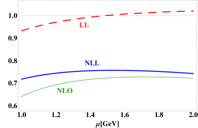
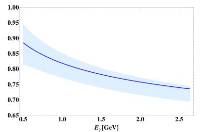
Figure 2: Left: Hard-collinear scale dependence of the radiative correction factor $[\lambda_{B}(1\,\mbox{GeV})/\lambda_{B}(\mu)]\times R(E_{\gamma},\mu)$ for $E_{\gamma}=2.0\,{\rm GeV}$. Right: Energy dependence with uncertainty band due to residual scale dependence.

The photon-energy dependence of the radiative correction factor is shown in the right panel of Fig. 2. The shaded band represents the theoretical uncertainty estimated from varying the hard-collinear scale in the interval $[1,2]\,\mbox{GeV}$ around the default value $\mu=1.5\,$GeV and the hard scales $\mu_{h1}=\mu_{h2}$ in $[m_{b}/2,2m_{b}]$ around $m_{b}$. The uncertainties from each variation are added in quadrature. We conclude that radiative corrections reduce the $B\to\gamma\ell\nu$ amplitude over the entire energy range, and more significantly at high photon energies.

Figure 3: Form factors $F_{V}(E_{\gamma})$, $F_{A}(E_{\gamma})$ and their difference. The bands show the total theoretical uncertainty, for fixed $\lambda_{B}(\mu_{0})=0.35\,$GeV.

The key quantities for the computation of differential decay distributions are the two form factors $F_{V}$, $F_{A}$ given in (2.9). We display them in Fig. 3, which summarizes our main theoretical result. To obtain the form factors we need an ansatz for the size and energy dependence of the symmetry-conserving form factor $\xi(E_{\gamma})$. The only information available is that it is a power correction of order $1/m_{b}$ to the leading term. We propose the form

$$\xi(E_{\gamma})=c\cdot\frac{f_{B}}{2E_{\gamma}}\,,$$ (3.2)

which features the same dependence on $E_{\gamma}$ as the leading term with $Q_{u}/\lambda_{B}$ replaced by $1/m_{b}$. The constant $c$ will be varied between $-1$ and $+1$. Fig. 3 displays $F_{V}$, $F_{A}$ and their difference including the theoretical uncertainty from adding in quadrature the scale uncertainty (as discussed above), the parameter $c$ and the input parameters from Tab. 1, except $\lambda_{B}$. We do not include the $\lambda_{B}$ variation into the error here, since we intend to use $B\to\gamma\ell\nu$ to determine $\lambda_{B}$. How well this can be done depends on the theoretical uncertainty in $F_{V}$, $F_{A}$ due to all other parameters. For comparison we also show in Fig. 3 the predicted form factors, when the hard scale $\mu_{h1}$ in the SCET matching coefficient is set to $2E_{\gamma}$ (dashed lines). The difference to the standard choice $\mu_{h1}=m_{b}$ becomes significant only at very small photon energies. Since the factorization approach requires $2E_{\gamma}\sim m_{b}$ the calculation of the form factors below photon energies of $1\,$GeV should certainly be considered unsafe.

Recall that both form factors are exactly equal at leading order in the heavy-quark expansion. The difference between the two curves referring to $F_{V}$ and $F_{A}$ is therefore a direct measure of the magnitude of power corrections, which indeed rises at smaller photon energies, where the calculation breaks down. It is interesting to note that $F_{V}$ is predicted to rise faster than $F_{A}$ towards small energies, which is compatible with a pole dominance ansatz to model the low-energy regime [1]. The uncertainties of $F_{V}$ and $F_{A}$ are highly correlated. This is seen explicitly when plotting the difference $F_{V}-F_{A}$ (lowest band in Fig. 3), which has a very small uncertainty. In fact, from (2.9) we obtain the definite prediction

$$F_{A}(E_{\gamma})-F_{V}(E_{\gamma})=\frac{f_{B}}{E_{\gamma}}\left[Q_{\ell}-\frac{Q_{b}m_{B}}{m_{b}}-\frac{Q_{u}m_{B}}{2E_{\gamma}}\right]$$ (3.3)

up to corrections of order $\alpha_{s}$. Thus, the form-factor difference depends only on $f_{B}$. It would be very interesting to test this prediction of a power-suppressed effect experimentally. Looking at (2.7) we see that this can be done by selecting events with $x_{\nu}\approx 1$, i.e. where the neutrino has nearly maximal energy and recoils against the lepton and the photon. Requiring a minimum separation angle between the lepton and the photon removes the non-radiative $B^{-}\to\ell\bar{\nu}$ contribution, which is, however, very small for the electron final state. Since $F_{V}-F_{A}$ is suppressed relative to $F_{V}+F_{A}$ the loss of statistics does not allow this test to be performed presently, but it should be within reach of the SuperB factories.

As $F_{V/A}\propto 1/\lambda_{B}$ approximately, a measurement of the two form factors through $B\to\gamma\ell\nu$ can easily be turned into a determination of $\lambda_{B}$, within the uncertainties of the theoretical prediction shown in Fig. 3. At present only upper limits exist on the branching fraction, resulting in lower bounds on $\lambda_{B}$ rather than a determination. We discuss the present limits and the dependence of partial branching fractions on $\lambda_{B}$ in the following.

4 Bound on $\lambda_{B}$ from (partial) branching fractions

Experimental studies of the radiative leptonic decay have been performed by the CLEO Collaboration [28] and, more recently, by the BABAR Collaboration [10, 11]. The BABAR analyses make use of partial branching fractions

$$\Delta\mathcal{B}=\tau_{B_{d}}\int\limits_{\text{PS-Cuts}}\!\!\!{\rm d}E_{\gamma}\;\!{\rm d}E_{\ell}\;\;\frac{\!{\rm d}^{2}\Gamma}{\!{\rm d}E_{\gamma}\;\!{\rm d}E_{\ell}}\,.$$ (4.1)

The first analysis [10] employs the cuts $E_{\ell}\in(1.875,2.64)\,{\rm GeV}$, $E_{\gamma}\in({0.45},2.35)\,{\rm GeV}$, $\cos\theta(\ell,\gamma)<-0.36$ in the cms frame of the $e^{+}e^{-}$ collision, and quotes $\Delta\mathcal{B}_{1}<1.7\,(2.3)\times 10^{-6}$ at 90% CL for flat priors on the amplitude (branching fraction). The second, published analysis [11] imposes only $E_{\gamma}<1\,\mbox{GeV}$ and yet finds the much weaker limit $\Delta\mathcal{B}_{2}<14\times 10^{-6}$. However, both analyses compare to a theoretical prediction that omits radiative corrections and contains an incorrect and numerically rather different expression for the $1/m_{b}$ power corrections. In Fig. 4, left panel, we show our prediction for $\Delta\mathcal{B}_{1}$ including uncertainties (solid, with band) for given $\lambda_{B}$, and compare it to the approximation without power corrections (NLL, dashed) and further omitting radiative corrections (LO, dot-dashed). Both effects together reduce $\Delta\mathcal{B}_{1}$ by more than a factor of two.

We first revisit the analysis of [10]. In this work $f_{B}=216\,$MeV and the rather large value $|V_{ub}|=0.00431$ are used, which further magnifies the theoretical prediction. In our analysis we adopt $|V_{ub}|_{\,\rm excl.}$ given in Tab. 1, since all exclusive decays except $B\to\tau\nu$ tend to favor this smaller value. In Fig. 4 we show the two BABAR limits on $\Delta\mathcal{B}_{1}$ (straight lines). The lower limit on $\lambda_{B}\equiv\lambda_{B}(1\,\mbox{GeV})$ follows from intersecting the lower end of the theoretical prediction with the straight lines. We then find that $\lambda_{B}>310\,(274)\,\mbox{MeV}$ at $90\%$ CL compared to $\lambda_{B}>669\,(591)\,\mbox{MeV}$ given in [10]. With the larger value of $|V_{ub}|_{\,\rm incl.}$ derived from inclusive semi-leptonic decays given in Tab. 1 we obtain $\lambda_{B}>372\,(331)\,\mbox{MeV}$, which is still significantly smaller that the previous values, and illustrates the importance of radiative and power corrections. The definition of $\Delta\mathcal{B}_{1}$ is far from ideal from the theoretical point of view, since it includes photons with energies down to $0.45\,$GeV, where the theoretical prediction is not valid. The above limits should therefore be taken with a grain of salt. In this respect, $\Delta\mathcal{B}_{2}$ is somewhat better suited, but the weak experimental limit [11] results in the rather weak limit $\lambda_{B}>115\,\mbox{MeV}$.

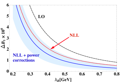
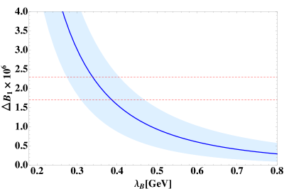
Figure 4: Dependence of the partial branching fraction $\Delta\mathcal{B}_{1}$ on $\lambda_{B}$. Left: LO (dot-dashed), NLL without (with) power corrections (dotted, solid). Right: Theoretical prediction compared to BABAR limits [10].

We conclude that present data does not yet allow us to put significant constraints on $\lambda_{B}$. However, the theoretical prediction of the form factors is sufficiently accurate such that $B\to\gamma\ell\nu$ holds great promise for the future. In Fig. 5 we show the inclusive branching fraction for a photon-energy cut $E_{\gamma}>1\,$GeV (upper band, equal to $\Delta\mathcal{B}_{2}$) and $E_{\gamma}>1.7\,$GeV, the latter being on more solid grounds theoretically. We see that a hypothetical measurement of $\mbox{Br}\,(B^{-}\to\gamma\ell\bar{\nu},E_{\gamma}>1.7\,\mbox{GeV})=2.0\times 10^{-6}$ with a 20% error would constrain $\lambda_{B}$ to $[167,304]\,$MeV with a central value of $228\,$MeV.

Can this be improved? The dominant theoretical errors arise from $\xi(E_{\gamma})$, and the inverse-logarithmic moments $\sigma_{1}$, $\sigma_{2}$. It is hard to conceive of theoretical tools that would determine these quantities without providing $\lambda_{B}$ itself, rendering the present analysis superfluous. From (2.14) we see that $\sigma_{1}$ influences the shape of the normalized photon-energy spectrum. But this dependence is rather weak when the photon-energy cut is large enough to be solidly in the perturbative regime, making an extraction of $\sigma_{1}$ difficult. We should mention though, that our error bands are based on rather conservative error ranges. For instance, we increased the error on $\sigma_{1}$ given in [9] by a factor of 2.5, since this is the only attempt to estimate $\sigma_{1}$ up to now.

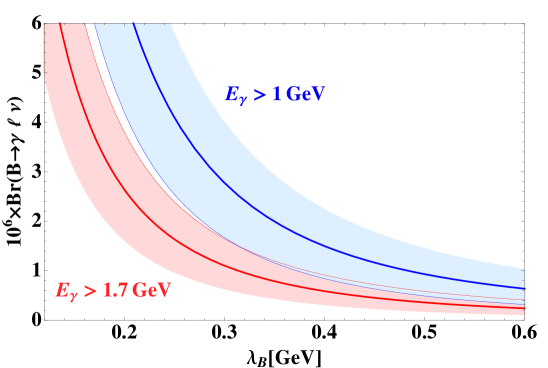
Figure 5: The partial branching fractions $\mbox{Br}\,(B^{-}\!\to\gamma\ell\bar{\nu},E_{\gamma}>E_{\rm cut})$ for $E_{\rm cut}=1\,$GeV (upper band) and $1.7\,$GeV (lower band).

5 Conclusion

We analyzed the radiative leptonic $B^{-}\to\gamma\ell\bar{\nu}$ decay with respect to its utility for determining the $B$ meson light-cone distribution amplitude, in particular its inverse moment, $\lambda_{B}$. We presented predictions for the form factors $F_{V}$, $F_{A}$ governing this decay, including for the first time radiative corrections and the leading-power corrections, and detailed uncertainty estimates. Corrections to the leading-order prediction reduce the branching fraction significantly. The BABAR upper limits on $B^{-}\to\gamma\ell\bar{\nu}$ therefore presently do not allow to put stringent constraints on $\lambda_{B}$. We also showed that the power-suppressed difference of the two form factors can be predicted at leading order. The hundred-fold increase in statistics available to future $B$ factories therefore makes $B^{-}\to\gamma\ell\bar{\nu}$ an interesting process for determining $\lambda_{B}$ and testing the theory of power corrections in hard, exclusive $B$ decays.

Acknowledgements

We thank S. Jäger for helpful comments. This work is supported in part by the DFG Sonderforschungsbereich/Transregio 9 “Computergestützte Theoretische Teilchenphysik”.

Appendix A Renormalization group evolution factor

The summation of formally large logarithms from the hard-to-hard-collinear scale ratio is accomplished by the renormalization group equation for the hard matching coefficients, or, equivalently the evolution factor $U(E_{\gamma},\mu_{h1},\mu_{h2},\mu)=U_{1}(E_{\gamma},\mu_{h1},\mu)U_{2}(\mu_{h2},\mu)^{-1}$. The first factor is associated with the running of the SCET current $\bar{\xi}W_{c}\gamma_{\mu_{\perp}}h_{v}$ and satisfies [5]

$$\mu\frac{d}{d\mu}\,U_{1}(E_{\gamma},\mu_{h},\mu)=\left(\Gamma_{\rm cusp}(\alpha_{s})\,\ln\frac{\mu}{2E_{\gamma}}+\gamma(\alpha_{s})\right)U_{1}(E_{\gamma},\mu_{h},\mu)$$ (A.1)

with initial condition $U_{1}(\mu,\mu)=1$. We expand the anomalous dimension and the QCD beta-function according to

$$\gamma(\alpha_{s})=\sum_{n=0}\gamma_{n}\left(\frac{\alpha_{s}}{4\pi}\right)^{n+1}\,\qquad\beta(\alpha_{s})=\mu\frac{d\alpha_{s}}{d\mu}=-2\alpha_{s}\sum_{n=0}\beta_{n}\left(\frac{\alpha_{s}}{4\pi}\right)^{n+1}$$ (A.2)

(similarly for $\Gamma_{\rm cusp}$). The solution to (A.1) is

$$U_{1}(E_{\gamma},\mu_{h},\mu) = \exp\left(\,\int_{\alpha_{s}(\mu_{h})}^{\alpha_{s}(\mu)}d\alpha_{s}\,\left[\frac{\gamma(\alpha_{s})}{\beta(\alpha_{s})}+\frac{\Gamma_{\rm cusp}(\alpha_{s})}{\beta(\alpha_{s})}\left(\ln\frac{2E_{\gamma}}{\mu_{h}}-\int_{\alpha_{s}(\mu_{h})}^{\alpha_{s}}\frac{d\alpha_{s}^{\prime}}{\beta(\alpha_{s}^{\prime})}\right)\right]\right)$$ (A.3)

$$=\,\exp\left(\,-\frac{\Gamma_{0}}{4\beta_{0}^{2}}\left(\frac{4\pi}{\alpha_{s}(\mu_{h})}\left[\ln r-1+\frac{1}{r}\right]-\frac{\beta_{1}}{2\beta_{0}}\,\ln^{2}r+\left(\frac{\Gamma_{1}}{\Gamma_{0}}-\frac{\beta_{1}}{\beta_{0}}\right)\left[r-1-\ln r\right]\right)\right)$$

$$\times\,\left(\frac{2E_{\gamma}}{\mu_{h}}\right)^{-\frac{\Gamma_{0}}{2\beta_{0}}\ln r}r^{-\frac{\gamma_{0}}{2\beta_{0}}}\times\Bigg{[}1-\frac{\alpha_{s}(\mu_{h})}{4\pi}\,\frac{\Gamma_{0}}{4\beta_{0}^{2}}\,\bigg{(}\frac{\Gamma_{2}}{2\Gamma_{0}}\left[1-r\right]^{2}+\frac{\beta_{2}}{2\beta_{0}}\left[1-r^{2}+2\ln r\right]$$

$$-\,\frac{\Gamma_{1}\beta_{1}}{2\Gamma_{0}\beta_{0}}\left[3-4r+r^{2}+2r\ln r\right]+\frac{\beta_{1}^{2}}{2\beta_{0}^{2}}\left[1-r\right]\left[1-r-2\ln r\right]\bigg{)}$$

$$+\,\frac{\alpha_{s}(\mu_{h})}{4\pi}\left(\ln\frac{2E_{\gamma}}{\mu_{h}}\left(\frac{\Gamma_{1}}{2\beta_{0}}-\frac{\Gamma_{0}\beta_{1}}{2\beta_{0}^{2}}\right)+\frac{\gamma_{1}}{2\beta_{0}}-\frac{\gamma_{0}\beta_{1}}{2\beta_{0}^{2}}\right)\left[1-r\right]+{\cal O}(\alpha_{s}^{2})\Bigg{]}$$

with $r=\alpha_{s}(\mu)/\alpha_{s}(\mu_{h})$. After the second equality the exact solution has been expanded to NLL. At this order the cusp anomalous dimension enters at the three-loop order [29]. Its series coefficients are

$$\Gamma_{0}=4C_{F},\qquad\Gamma_{1}=C_{F}\left[\frac{268}{3}-4\pi^{2}-\frac{40}{9}n_{l}\right],$$ (A.4)

$$\Gamma_{2}=C_{F}\left[1470-\frac{536\pi^{2}}{3}+\frac{44\pi^{4}}{5}+264\zeta(3)+n_{l}\left(-\frac{1276}{9}+\frac{80\pi^{2}}{9}-\frac{208}{3}\zeta(3)\right)-\frac{16}{27}n_{l}^{2}\right],$$

where $n_{l}=4$ is the number of light fermion flavours (the charm quark is treated as massless), and $C_{F}=4/3$ the quadratic Casimir of the fundamental SU(3) representation. The remaining anomalous dimension of the SCET heavy-light current is needed at two loops, and given by

$$\gamma_{0}=-5C_{F},\qquad\gamma_{1}=C_{F}\left[-\frac{1585}{18}-\frac{5\pi^{2}}{6}+34\zeta(3)+n_{l}\left(\frac{125}{27}+\frac{\pi^{2}}{3}\right)\right]\,.$$ (A.5)

The two-loop expression is given explicitly in [18, 20] confirming an earlier conjecture [30].

The second evolution factor $U_{2}(\mu_{h2},\mu)$ arises from the matching of the $B$ meson decay constants in QCD and heavy-quark effective theory (HQET). Its expression follows from the ones given above by setting the cusp anomalous dimension to zero, and by replacing $\gamma_{i}$ by the anomalous dimension of the heavy-light current in HQET, $\gamma_{i,\rm hl}$, given to two loops by [31, 32]

$$\gamma_{0,\rm hl}=-3C_{F},\qquad\gamma_{1,\rm hl}=C_{F}\left[-\frac{127}{6}-\frac{14\pi^{2}}{9}+\frac{5}{3}n_{l}\right]\,.$$ (A.6)

The three-loop evolution of the strong coupling in the $\overline{\rm MS}$ scheme is computed from

$$\alpha_{s}(\mu) = \frac{4\pi}{\beta_{0}\ln(\mu^{2}/\Lambda^{2})}\Bigg{[}1-\frac{\beta_{1}}{\beta_{0}^{2}}\frac{\ln\ln(\mu^{2}/\Lambda^{2})}{\ln(\mu^{2}/\Lambda^{2})}+\frac{\beta_{1}^{2}}{\beta_{0}^{4}\ln^{2}(\mu^{2}/\Lambda^{2})}$$ (A.7)

$$\times\,\left(\left(\ln\ln(\mu^{2}/\Lambda^{2})-\frac{1}{2}\right)^{2}+\frac{\beta_{2}\beta_{0}}{\beta_{1}^{2}}-\frac{5}{4}\right)\Bigg{]}$$

with

$$\beta_{0}=11-\frac{2n_{l}}{3},\qquad\beta_{1}=102-\frac{38n_{l}}{3}\,\qquad\beta_{2}=\frac{2857}{2}-\frac{5033}{18}n_{l}+\frac{325}{54}n_{l}^{2}.$$ (A.8)

References

- [1] D. Becirevic, B. Haas, E. Kou, Phys. Lett. B681 (2009) 257-263, arXiv:0907.1845 [hep-ph].
- [2] G. P. Korchemsky, D. Pirjol, T. -M. Yan, Phys. Rev. D61 (2000) 114510, hep-ph/9911427.
- [3] S. Descotes-Genon, C. T. Sachrajda, Nucl. Phys. B650 (2003) 356-390, hep-ph/0209216.
- [4] E. Lunghi, D. Pirjol, D. Wyler, Nucl. Phys. B649 (2003) 349-364, hep-ph/0210091.
- [5] S. W. Bosch, R. J. Hill, B. O. Lange, M. Neubert, Phys. Rev. D67 (2003) 094014, hep-ph/0301123.
- [6] A. G. Grozin, M. Neubert, Phys. Rev. D55 (1997) 272-290, hep-ph/9607366.
- [7] M. Beneke, G. Buchalla, M. Neubert, C. T. Sachrajda, Phys. Rev. Lett. 83 (1999) 1914-1917, hep-ph/9905312; Nucl. Phys. B591 (2000) 313-418, hep-ph/0006124.
- [8] M. Beneke, T. Feldmann, Nucl. Phys. B592 (2001) 3-34, hep-ph/0008255.
- [9] V. M. Braun, D. Yu. Ivanov, G. P. Korchemsky, Phys. Rev. D69 (2004) 034014, hep-ph/0309330.
- [10] B. Aubert et al. [ BABAR Collaboration ], arXiv:0704.1478 [hep-ex].
- [11] B. Aubert et al. [ BABAR Collaboration ], Phys. Rev. D80 (2009) 111105, arXiv:0907.1681 [hep-ex].
- [12] M. Beneke, S. Jäger, Nucl. Phys. B751 (2006) 160-185, hep-ph/0512351.
- [13] G. Bell, V. Pilipp, Phys. Rev. D80 (2009) 054024, arXiv:0907.1016 [hep-ph].
- [14] M. Beneke, T. Huber, X. -Q. Li, Nucl. Phys. B832 (2010) 109-151, arXiv:0911.3655 [hep-ph].
- [15] A. Khodjamirian, D. Wyler, In *Gurzadyan, V.G. (ed.) et al.: From integrable models to gauge theories* 227-241, hep-ph/0111249.
- [16] Y. -Y. Charng, H. -n. Li, Phys. Rev. D72 (2005) 014003, hep-ph/0505045.
- [17] R. Bonciani, A. Ferroglia, JHEP 0811 (2008) 065, arXiv:0809.4687 [hep-ph].
- [18] H. M. Asatrian, C. Greub, B. D. Pecjak, Phys. Rev. D78 (2008) 114028, arXiv:0810.0987 [hep-ph].
- [19] M. Beneke, T. Huber, X. -Q. Li, Nucl. Phys. B811 (2009) 77-97, arXiv:0810.1230 [hep-ph].
- [20] G. Bell, Nucl. Phys. B812 (2009) 264-289, arXiv:0810.5695 [hep-ph].
- [21] C. W. Bauer, S. Fleming, D. Pirjol, I. W. Stewart, Phys. Rev. D63 (2001) 114020, hep-ph/0011336.
- [22] C. W. Bauer, D. Pirjol, I. W. Stewart, Phys. Rev. D65 (2002) 054022, hep-ph/0109045.
- [23] M. Beneke, A. P. Chapovsky, M. Diehl, T. Feldmann, Nucl. Phys. B643, 431-476 (2002) 431-476, hep-ph/0206152.
- [24] M. Beneke, T. Feldmann, Phys. Lett. B553 (2003) 267-276, hep-ph/0211358.
- [25] M. Beneke, T. Feldmann, Nucl. Phys. B685 (2004) 249-296, hep-ph/0311335.
- [26] M. Beneke, C. Hellmann, J. Rohrwild, work in progress.
- [27] B. O. Lange, M. Neubert, Phys. Rev. Lett. 91 (2003) 102001, hep-ph/0303082.
- [28] T. E. Browder et al. [ CLEO Collaboration ], Phys. Rev. D56 (1997) 11-16.
- [29] S. Moch, J. A. M. Vermaseren, A. Vogt, Nucl. Phys. B688 (2004) 101-134, hep-ph/0403192.
- [30] M. Neubert, Eur. Phys. J. C40 (2005) 165-186, hep-ph/0408179.
- [31] X. -D. Ji, M. J. Musolf, Phys. Lett. B257 (1991) 409-413.
- [32] D. J. Broadhurst, A. G. Grozin, Phys. Lett. B267 (1991) 105-110, hep-ph/9908362.