Plumes in kinetic transport: how the simple random walk can be too simple

Abstract.

We consider a discrete time particle model for kinetic transport on the two dimensional integer lattice. The particle can move due to advection in the $x$-direction and due to dispersion. This happens when the particle is free, but it can also be adsorbed and then does not move. When the dispersion of the particle is modeled by simple random walk, strange phenomena occur. In the second half of the paper, we resolve these problems and give expressions for the shape of the plume consisting of many particles.

Key words. simple random walk, conditional variance, reactive transport, kinetic adsorption, double-peak.

MSC: 60J20, 60J10

1. Introduction

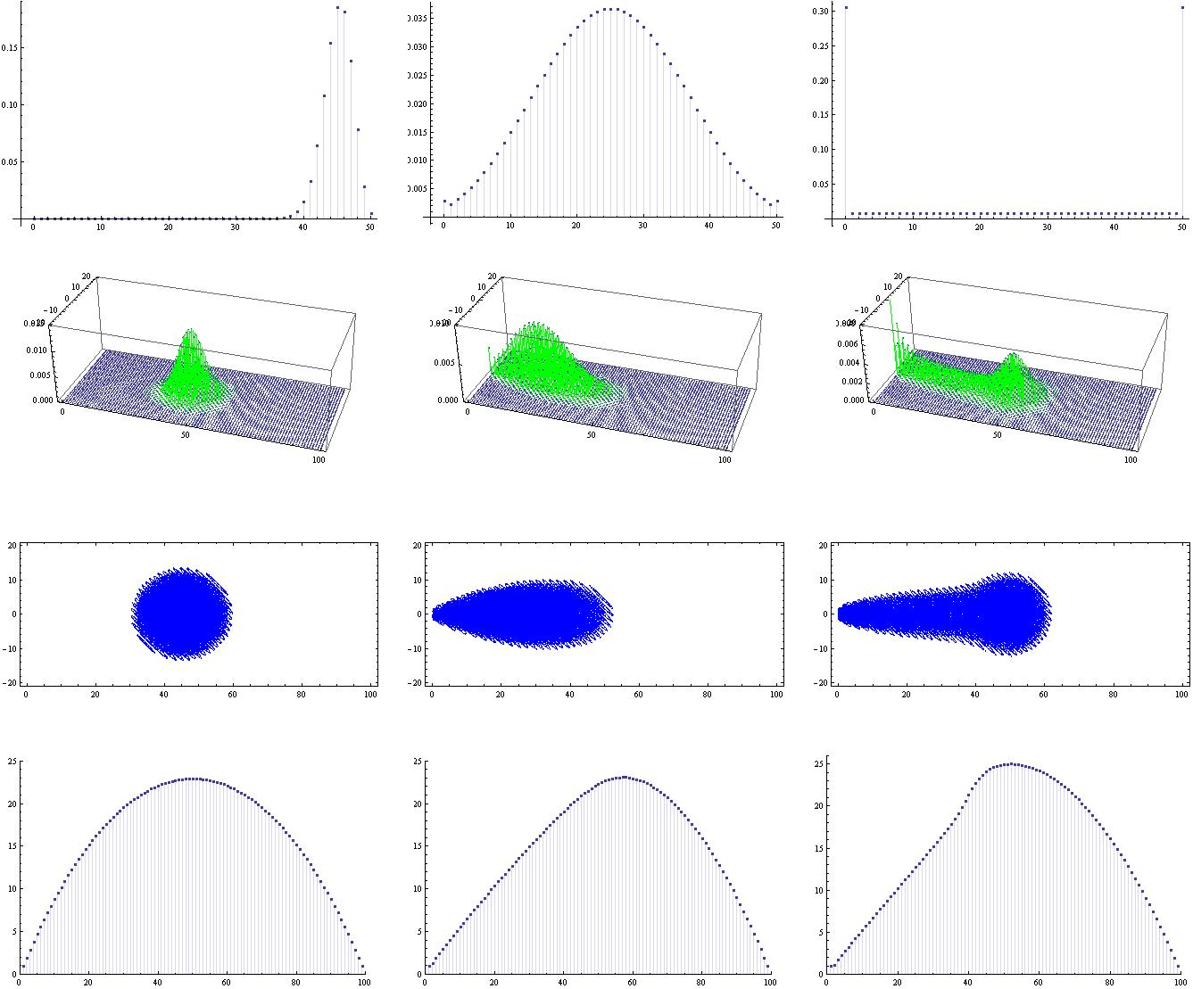
We consider a discrete time two dimensional stochastic kinetic transport model, which is described by a two dimensional random walk with a drift in the $x$ direction. Here the kinetics refers to the possibility that the particle may be adsorbed and released at random times, slowing down the movement of the particle. Let $S(n)=(S_{X}(n),S_{Y}(n))$ be the position of the particle at time $n=0,1,\dots$. In the engineering literature (see e.g. [3]) simulations are performed with a large number of particles independently performing such a slowed down random walk. This results in a plume of particles, and there is interest in the shape of this plume. One of the remarkable phenomena is that level sets of the concentration function of the plume need not be convex (see Figure 1, last column).

A natural quantitative way to measure the lateral spread of the plume at position $x$ at time $n$ is to consider $\sigma^{2}_{x}={\rm Var}\left(S_{Y}(n)~{}|~{}S_{X}(n)=x\right)$. The goal of our paper is to compute this conditional variance, and to discuss its properties. Intuitively, $\sigma^{2}_{x}$ should be increasing in $x$. However, if we model the random walk with the natural choice: the simple symmetric random walk on the 2D integer lattice, then (see Figure 1, bottom row) this is not the case, as we prove in Section 3. A second strange phenomenon that we observe here is that there is symmetry (i.e., $\sigma^{2}_{x}=\sigma^{2}_{2n-x}$) when the total number of times the particle has been free follows a binomial distribution (see Figure 1, bottom left). The background for this is a symmetry property of the asymmetric 2D simple random walk, as we show in Section 4.

In Section 5 we get rid of the strange behaviour caused by the simple random walk by tilting the steps. We also show that this choice is ‘right’, as we obtain the same behaviour in the case of Gaussian distributions for the random walk.

For related work lying at the basis of the present paper, see [5].

Figure 1. The probability mass function $f_{50}$ of $K_{50}$, the probability mass function of $S(50)$, a list contour plot of its mass function and the conditional variance ${\rm Var}\left(S_{Y}(50)~{}|~{}S_{X}(50)=x\right)$ with $\nu=\pi,\alpha=\beta=1/4$. In the first column $a=0.1,b=0.9$; in the second column $a=b=0.1$; in the last column $a=b=0.01$. See Section 2 and Example 3.1 for further explanations.

2. A discrete time stochastic model for kinetic transport

The kinetic transport model is built out of two independent processes: a 2D random walk $\{(X_{k},Y_{k}),\,k\geq 1\}$, and a two-state Markov chain $\{Z_{k},\,k\geq 1\}$ (see [2] for the 1D case). We denote by $\rm{P}$ the probability measure on a large enough space to accomodate both processes. The two processes describe the behavior of a single particle that in each unit time interval can only be in one of two states: ‘free’ or ‘adsorbed’, coded by the letters F and A. The particle can only move when it is ‘free’, and in this case its displacement has two components: dispersion and advection.

Let $(X_{k},Y_{k})$ be the displacement of the particle due to the dispersion the $k$th time that it is ‘free’. We model the $(X_{k},Y_{k})$ as independent identically distributed random vectors satisfying

(1) $${\rm P}\left((X_{k},Y_{k})=(j,0)\right)=\alpha,\quad{\rm P}\left((X_{k},Y_{k})=(0,j)\right)=\beta\quad\textrm{for}~{}j=\pm 1$$

where $\alpha,\beta\geq 0,\;\alpha+\beta=1/2$. This means that the particle moves one unit to the left or the right with the same probability $\alpha$, and moves one unit up or down with the same probability $\beta$. When the particle is free, the displacement during a unit time interval due to advection is given by one unit in the $x$ direction.

The kinetics, i.e., the movement from ‘free’ to ‘adsorbed’ and vice versa, is modeled by a Markov chain $\{Z_{k},k\geq 1\}$ on the two states $\{{\textsc{F}},{\textsc{A}}\}$ with initial distribution $\nu=(\nu_{\textsc{F}},\nu_{\textsc{A}})$ and transition matrix

(2) $$\left[{\begin{array}[]{*{20}c}{p_{{\textsc{F}},{\textsc{F}}}}&{p_{{\textsc{F}},{\textsc{A}}}}\\ {p_{{\textsc{A}},{\textsc{F}}}}&{p_{{\textsc{A}},{\textsc{A}}}}\\ \end{array}}\right]=\left[{\begin{array}[]{*{20}c}1-a&a\\ b&{1-b}\\ \end{array}}\right].$$

Clearly the stationary distribution $\pi=(\pi_{\textsc{F}},\pi_{\textsc{A}})$ of the Markov chain $\{Z_{k}\}$ is given by $\pi_{\textsc{F}}=b/(a+b)$ and $\pi_{\textsc{A}}=a/(a+b).$ Let $K_{n}$ be the occupation time of the process $\{Z_{k}\}$ in state F up to time $n$, i.e.,

$$K_{n}=\sum_{k=1}^{n}{\bf 1}_{\{Z_{k}={\textsc{F}}\}}.$$

Then the distribution of $K_{n}$ is well known, and is called a Markov binomial distribution (see, e.g., [1, 4]). Let $f_{n}$ be its distribution, i.e., $f_{n}(k)={\rm P}\left(K_{n}=k\right)$ for $0\leq k\leq n$. Then it is easy to calculate $f_{n}(k)$ by the following recurrence equation

$$f_{n+2}(k+1)=(1-b)f_{n+1}(k+1)+(1-a)f_{n+1}(k)-(1-a-b)f_{n}(k)$$

with initial conditions

$$\begin{split}f_{1}(0)=\nu_{\textsc{A}},~{}f_{1}(1)=\nu_{\textsc{F}},~{}f_{2}(0)=\nu_{\textsc{A}}(1-b),~{}f_{2}(1)=\nu_{\textsc{A}}b+\nu_{\textsc{F}}a,~{}f_{2}(2)=\nu_{\textsc{F}}(1-a).\end{split}$$

Now let $S(n)$ be the position of the particle at time $n$, where $S(0)=(0,0)$. Then by the above we can write $S(n)$ for $n\geq 1$ as

$$S(n)=(S_{X}(n),S_{Y}(n))=\sum_{k=1}^{K_{n}}(X_{k}+1,Y_{k}).$$

3. Conditional variance

In this section we are interested in the conditional variance of $S_{Y}(n)$ given $S_{X}(n)=x$. For a real number $c\in\mathbb{R}$, let $\lfloor c\rfloor$ be the largest integer less than or equal to $c$, and $\lceil c\rceil$ be the least integer greater than or equal to $c$. For two real numbers $c$ and $d$, let $c\vee d:=\max\{c,d\}$ and $c\wedge d:=\min\{c,d\}.$

Proposition 3.1.

For $n\geq 1$, and $0\leq x\leq 2n,-n\leq y\leq n$, we have for $x\equiv y\mod{2}$

$$\begin{split}{\rm P}\left(S(n)=(x,y)\right)=\sum_{k=\lceil x/2\rceil}^{n}f_{n}(k)\sum_{j=0\vee(x-k)}^{\frac{x+y}{2}\wedge\frac{x-y}{2}}\frac{k!\;\;\alpha^{2j+k-x}\beta^{x-2j}}{j!\,(j+k-x)!\,((x+y)/2-j)!\,((x-y)/2-j)!},\end{split}$$

and ${\rm P}\left(S(n)=(x,y)\right)=0$ for $x\not\equiv y\mod 2$.

Proof.

For $0\leq x\leq 2n$ and $-n\leq y\leq n$, we consider the probability of the particle being at position $(x,y)$ at time $n$, conditioned on $K_{n}=k$. Let $\overline{x}\,(\underline{x},\,\overline{y},\,\underline{y})$ be the number of rightwards (leftwards, upwards, downwards) steps of the random walk $S_{k}=(X_{1}+\cdots+X_{k}+k,Y_{1}+\cdots+Y_{k})$. Suppose the walk makes $\overline{x}=j$ steps to the right. On the event $\{S_{k}=(x,y)\}$ we then have

$$\left\{\begin{array}[]{l}\overline{x}=j\\ \overline{x}-\underline{x}=x-k\\ \overline{y}-\underline{y}=y\\ \overline{x}+\underline{x}+\overline{y}+\underline{y}=k\end{array}\right.\quad\Longrightarrow\quad\left\{\begin{array}[]{l}\overline{x}=j\\ \underline{x}=j+k-x\\ \overline{y}=(x+y)/2-j\\ \underline{y}=(x-y)/2-j.\end{array}\right.$$

Necessarily, $x\equiv y\mod 2$. Since $\overline{x},\,\underline{x},\,\overline{y},\,\underline{y}\geq 0$, it immediately follows that

$$\max\{0,x-k\}\leq j\leq\min\Big{\{}\frac{x+y}{2},\frac{x-y}{2}\Big{\}}.$$

By a standard combinatorial analysis, and using Equation (1) we see that

$$\begin{split}{\rm P}\left(S(n)=(x,y)~{}|~{}K_{n}=k\right)&={\rm P}\left(S_{k}=(x,y)\right)\\ &=\sum_{0\vee(x-k)}^{\frac{x+y}{2}\wedge\frac{x-y}{2}}\frac{k!\;\;\alpha^{2j+k-x}\beta^{x-2j}}{j!\,(j+k-x)!\,((x+y)/2-j)!\,((x-y)/2-j)!}.\end{split}$$

Clearly $x\leq 2k$, yielding that $k\geq\lceil x/2\rceil$. Multiplying by $f_{n}(k)$, and adding over $k$ ranging from $\lceil x/2\rceil$ to $n$, completes the proof of the proposition. ∎

Proposition 3.2.

For $n\geq 1$ and $0\leq x\leq 2n$, the conditional variance is given by

$$\begin{split}{\rm Var}\left(S_{Y}(n)~{}|~{}S_{X}(n)=x\right)=\frac{\sum\limits_{k=\lceil x/2\rceil}^{n}f_{n}(k)\sum\limits_{j=0\vee(x-k)}^{\lfloor x/2\rfloor}(x-2j)\binom{k}{j,j+k-x,x-2j}\alpha^{2j+k-x}(2\beta)^{x-2j}}{\sum\limits_{k=\lceil x/2\rceil}^{n}f_{n}(k)\sum\limits_{j=0\vee(x-k)}^{\lfloor x/2\rfloor}\binom{k}{j,j+k-x,x-2j}\alpha^{2j+k-x}(2\beta)^{x-2j}}.\end{split}$$

where $\binom{m}{\ell,s,m-\ell-s}=\frac{m!}{\ell!\,s!\,(m-\ell-s)!}$ denotes a trinomial coefficient.

Proof.

In a similar way as in Proposition 3.1, we obtain that

$$\begin{split}{\rm P}\left(S_{X}(n)=x\right)&=\sum_{k=0}^{n}f_{n}(k){\rm P}\left(S_{X}(n)=x~{}|~{}K_{n}=k\right)\\ &=\sum_{k=\lceil x/2\rceil}^{n}f_{n}(k)\sum_{j=0\vee(x-k)}^{\lfloor x/2\rfloor}\frac{k!}{j!\,(j+k-x)!\,(x-2j)!}\alpha^{2j+k-x}(2\beta)^{x-2j}.\end{split}$$

By symmetry ${\rm E}\!\left[S_{Y}(n)~{}|~{}S_{X}(n)=x\right]=0$. So

$$\begin{split}{\rm Var}\left(S_{Y}(n)~{}|~{}S_{X}(n)=x\right)=\sum_{\stackrel{{\scriptstyle y\equiv x\mod 2}}{{-n\leq y\leq n}}}y^{2}{\rm P}\left(S_{Y}(n)=y~{}|~{}S_{X}(n)=x\right),\end{split}$$

and the proposition follows by using Proposition 3.1 in the following calculation

$$\begin{split}&\sum_{\stackrel{{\scriptstyle y\equiv x\mod 2}}{{-n\leq y\leq n}}}y^{2}{\rm P}\left(S(n)=(x,y)\right)\\ =&~{}\sum\limits_{k=\lceil x/2\rceil}^{n}f_{n}(k)\sum\limits_{j=0\vee(x-k)}^{\lfloor x/2\rfloor}\frac{k!}{j!\,(j+k-x)!\,(x-2j)!}\alpha^{2j+k-x}\beta^{x-2j}\sum_{\stackrel{{\scriptstyle y\equiv x\mod 2}}{{-n\leq y\leq n}}}y^{2}\binom{x-2j}{\frac{x-y}{2}-j}\\ =&~{}\sum\limits_{k=\lceil x/2\rceil}^{n}f_{n}(k)\sum\limits_{j=0\vee(x-k)}^{\lfloor x/2\rfloor}\frac{k!}{j!\,(j+k-x)!\,(x-2j)!}\alpha^{2j+k-x}\beta^{x-2j}\sum_{s=0}^{x-2j}(x-2j-2s)^{2}\binom{x-2j}{s}\\ =&~{}\sum\limits_{k=\lceil x/2\rceil}^{n}f_{n}(k)\sum\limits_{j=0\vee(x-k)}^{\lfloor x/2\rfloor}(x-2j)\frac{k!}{j!\,(j+k-x)!\,(x-2j)!}\alpha^{2j+k-x}(2\beta)^{x-2j},\end{split}$$

where the first equality follows from the usual convention $\binom{m}{\ell}=0$ for $\ell<0$ or $\ell>m$. ∎

Example 3.1.

Let $n=50,\alpha=\beta=1/4$, and the initial distribution $\nu=\pi.$ See Figure 1.

Note that the last column of Figure 1 shows that two peaks appear in the probability mass function of $S(n)$ when both $a$ and $b$ are small. This double peaking can be explained (see [2]) by the multimodality of the Markov binomial distribution, i.e., $\{f_{n}(k)\}_{k=0}^{n}$ can be bimodal or even trimodal when both $a$ and $b$ are small (see [1]).

4. A symmetry property of asymmetric random walk

The first column of Figure 1 suggests that when $a+b=1$ the conditional variance is symmetric. This is the content of the next proposition.

Proposition 4.1.

For $n\geq 1$ and $0\leq x\leq n$, if $\nu=\pi$ and $a+b=1$, we have

$${\rm Var}\left(S_{Y}(n)~{}|~{}S_{X}(n)=n+x\right)={\rm Var}\left(S_{Y}(n)~{}|~{}S_{X}(n)=n-x\right).$$

Proof.

For $\nu=\pi$ and $a+b=1$, the Markov chain $\{Z_{k}\}$ is trivial in the sense that $\{Z_{k}\}$ is independent identically distributed. Then the behavior of the particle is a random walk starting at position $(0,0)$ with the following transition probabilities for $k=0,1,\cdots,n-1,$

$$\begin{split}&{\rm P}\left(S(k+1)=S(k)+(2,0)\right)=b\alpha,\quad{\rm P}\left(S(k+1)=S(k)+(0,0)\right)=b\alpha+a,\\ &{\rm P}\left(S(k+1)=S(k)+(1,1)\right)={\rm P}\left(S(k+1)=S(k)+(1,-1)\right)=b\beta.\end{split}$$

For convenience we shift the random walk steps by adding $(-1,0)$ to them and let the particle start at position $(n,0)$. Then the corresponding transition probabilities of the random walk are given by

$$\begin{split}&{\rm P}\left(\hat{S}(k+1)=\hat{S}(k)+(1,0)\right)=b\alpha,\quad{\rm P}\left(\hat{S}(k+1)=\hat{S}(k)+(-1,0)\right)=b\alpha+a,\\ &{\rm P}\left(\hat{S}(k+1)=\hat{S}(k)+(0,1)\right)={\rm P}\left(\hat{S}(k+1)=\hat{S}(k)+(0,-1)\right)=b\beta.\end{split}$$

The result now follows from the following theorem with $\omega=b\alpha,\varepsilon=b\alpha+a$ and $\gamma=\delta=b\beta$. ∎

Theorem 4.1.

Let $(S_{n})=((S_{n}^{(1)},S_{n}^{(2)}))$ be a simple random walk in the plane, i.e., $S_{0}=(0,0)$ and $(S_{n})$ has increments $\mathcal{X}_{k}$ with

$${\mathbb{P}}\left(\mathcal{X}_{k}=(1,0)\right)=\omega,\quad{\mathbb{P}}\left(\mathcal{X}_{k}=(-1,0)\right)=\varepsilon,\quad{\mathbb{P}}\left(\mathcal{X}_{k}=(0,1)\right)=\gamma,\quad{\mathbb{P}}\left(\mathcal{X}_{k}=(0,-1)\right)=\delta,$$

where $\omega+\varepsilon+\gamma+\delta=1$. Then for $x=0,1,2,\dots,n$ and $-n\leq y\leq n$,

$${\mathbb{P}}\left(S_{n}^{(2)}=y~{}\big{|}~{}S_{n}^{(1)}=x\right)={\mathbb{P}}\left(S_{n}^{(2)}=y~{}\big{|}~{}S_{n}^{(1)}=-x\right).$$

Proof.

A similar combinatorial analysis as in the proof of Proposition 3.1 yields that for $x=0,1,\cdots,n$ and $-n\leq y\leq n$

$$\begin{split}{\mathbb{P}}\left(S_{n}^{(1)}=x,S_{n}^{(2)}=y\right)&=\sum_{j=0}^{\frac{n-x-y}{2}\wedge\frac{n-x+y}{2}}\frac{n!\;\;\omega^{j+x}\varepsilon^{j}\gamma^{(n-x-2j+y)/2}\delta^{(n-x-2j-y)/2}}{j!\,(j+x)!\,((n-x-y)/2-j)!\,((n-x+y)/2-j)!},\\ {\mathbb{P}}\left(S_{n}^{(1)}=-x,S_{n}^{(2)}=y\right)&=\sum_{j=0}^{\frac{n-x-y}{2}\wedge\frac{n-x+y}{2}}\frac{n!\;\;\omega^{j}\varepsilon^{j+x}\gamma^{(n-x-2j+y)/2}\delta^{(n-x-2j-y)/2}}{j!\,(j+x)!\,((n-x-y)/2-j)!\,((n-x+y)/2-j)!}\end{split}$$

if $y\equiv n-x\mod 2$, and ${\mathbb{P}}\left(S_{n}^{(1)}=x,S_{n}^{(2)}=y\right)={\mathbb{P}}\left(S_{n}^{(1)}=-x,S_{n}^{(2)}=y\right)=0$ if $y\not\equiv n-x\mod 2.$ Similarly,

$$\begin{split}{\mathbb{P}}\left(S_{n}^{(1)}=x\right)&=\sum_{i=0}^{\lfloor\frac{n-x}{2}\rfloor}\frac{n!}{i!\,(i+x)!\,(n-x-2i)!}\omega^{i+x}\varepsilon^{i}(\gamma+\delta)^{n-2i-x},\\ {\mathbb{P}}\left(S_{n}^{(1)}=-x\right)&=\sum_{i=0}^{\lfloor\frac{n-x}{2}\rfloor}\frac{n!}{i!\,(i+x)!\,(n-x-2i)!}\omega^{i}\varepsilon^{i+x}(\gamma+\delta)^{n-2i-x}.\end{split}$$

Then it is easy to check that for $x=0,1,\cdots,n$ and $-n\leq y\leq n$

$$\begin{split}{\mathbb{P}}\left(S_{n}^{(1)}=x,S_{n}^{(2)}=y\right){\mathbb{P}}\left(S_{n}^{(1)}=-x\right)={\mathbb{P}}\left(S_{n}^{(1)}=-x,S_{n}^{(2)}=y\right){\mathbb{P}}\left(S_{n}^{(1)}=x\right),\end{split}$$

which finishes the proof of the theorem. ∎

5. Forty five degree dispersion

To fix the strange behavior observed when the dispersion is 2D simple random walk, we consider now a well known variant with increments

$${\rm P}\left((X_{k},Y_{k})=(1,j)\right)=\alpha,\quad{\rm P}\left((X_{k},Y_{k})=(-1,j)\right)=\beta\quad\textrm{for}~{}j=\pm 1,$$

where $\alpha,\beta\geq 0$ and $\alpha+\beta=1/2.$ Let $(\mathcal{S}(n))$ be the corresponding kinetic transport process.

Proposition 5.1.

For $n\geq 1$ and $0\leq x\leq n,-n\leq y\leq n$, the distribution of $\mathcal{S}(n)$ is given by

$${\rm P}\left(\mathcal{S}(n)=(2x,y)\right)=\sum_{k=x}^{n}f_{n}(k)\binom{k}{x}\binom{k}{\frac{k+y}{2}}\alpha^{x}\beta^{k-x},$$

and the conditional variance is given by

$${\rm Var}\left(\mathcal{S}_{Y}(n)~{}|~{}\mathcal{S}_{X}(n)=2x\right)=\frac{\sum_{k=x}^{n}kf_{n}(k)\binom{k}{x}(2\alpha)^{x}(2\beta)^{k-x}}{\sum_{k=x}^{n}f_{n}(k)\binom{k}{x}(2\alpha)^{x}(2\beta)^{k-x}}.$$

Proof.

The proof of the proposition is quite similar to that for Proposition 3.1. For $0\leq x\leq n$ and $-n\leq y\leq n$, we consider the probability of the particle being at position $(2x,y)$ at time $n$ by conditioning on $K_{n}=k$. In order to achieve $\mathcal{S}_{X}(n)=k+X_{1}+\cdots+X_{k}=2x$ the particle needs to move $x$ steps to the right and $k-x$ steps to the left. Also to obtain $\mathcal{S}_{Y}(n)=Y_{1}+\cdots Y_{k}=y$ the particle needs to move $(k+y)/2$ steps up and $(k-y)/2$ steps down. Let $j$ be the number of steps of type $(1,1)$, then the particle moves $x-j$ steps of type $(1,-1)$, $(k+y)/2-j$ steps of type $(-1,1)$, and the remaining $k-(j+x-j+(k+y)/2-j)=(k-y)/2-(x-j)$ steps of type $(-1,-1)$. To ensure the nonnegativity of all of these quantities, we have $x\leq k\leq n$ and $\max\{0,(y-k)/2+x\}\leq j\leq\min\{x,(k+y)/2\}$. We conclude by using Vandermonde’s identity, obtaining that for $0\leq x\leq n,-n\leq y\leq n$ and $k\equiv y\mod 2$

$${\rm P}\left(\mathcal{S}(n)=(2x,y)~{}|~{}K_{n}=k\right)=\sum_{j=0}^{(k+y)/2}\binom{k}{x}\binom{x}{j}\binom{k-x}{\frac{k+y}{2}-j}\alpha^{x}\beta^{k-x}=\binom{k}{x}\binom{k}{\frac{k+y}{2}}\alpha^{x}\beta^{k-x}.$$

For the conditional variance ${\rm Var}\left(\mathcal{S}_{Y}(n)~{}|~{}\mathcal{S}_{X}(n)=2x\right)$, we still need the probability of the particle being at position $2x$ at time $n$. In a similar way as above it follows that

$${\rm P}\left(\mathcal{S}_{X}(n)=2x~{}|~{}K_{n}=k\right)=\binom{k}{x}(2\alpha)^{x}(2\beta)^{k-x}.$$

By symmetry ${\rm E}\!\left[\mathcal{S}_{Y}(n)~{}|~{}\mathcal{S}_{X}(n)=2x\right]=0$. So

$${\rm Var}\left(\mathcal{S}_{Y}(n)~{}|~{}\mathcal{S}_{X}(n)=2x\right)=\sum_{y=-n}^{n}y^{2}{\rm P}\left(\mathcal{S}_{Y}(n)=y~{}|~{}\mathcal{S}_{X}(n)=2x\right),$$

and the proposition follows by the following calculation

$$\begin{split}&\sum_{y=-n}^{n}y^{2}{\rm P}\left(\mathcal{S}(n)=(2x,y)\right)=\sum_{y=-n}^{n}y^{2}\sum_{\stackrel{{\scriptstyle k\equiv y\mod 2}}{{x\leq k\leq n}}}f_{n}(k)\binom{k}{x}\binom{k}{\frac{k+y}{2}}\alpha^{x}\beta^{k-x}\\ =&~{}\sum_{k=x}^{n}f_{n}(k)\binom{k}{x}\alpha^{x}\beta^{k-x}\sum_{\stackrel{{\scriptstyle y\equiv k\mod 2}}{{-n\leq y\leq n}}}y^{2}\binom{k}{\frac{k+y}{2}}=\sum_{k=x}^{n}f_{n}(k)\binom{k}{x}\alpha^{x}\beta^{k-x}\sum_{s=0}^{k}(k-2s)^{2}\binom{k}{s}\\ =&~{}\sum_{k=x}^{n}kf_{n}(k)\binom{k}{x}(2\alpha)^{x}(2\beta)^{k-x}.\end{split}$$

∎

Example 5.1.

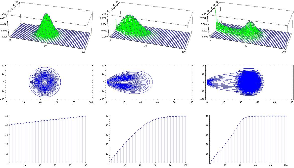
Let $n=50,\alpha=\beta=1/4$, and the initial distribution $\nu=\pi$. See Figure 2.

Figure 2. The probability mass function of $\mathcal{S}(50)$, a list contour plot of its mass function and the conditional variance ${\rm Var}\left(\mathcal{S}_{Y}(50)~{}|~{}\mathcal{S}_{X}(50)=2x\right)$ with $\nu=\pi,\alpha=\beta=1/4$. In the first column $a=0.1,b=0.9$; in the second column $a=b=0.1$; in the last column $a=b=0.01$.

Figure 2 suggests that the conditional variance ${\rm Var}\left(\mathcal{S}_{Y}(n)~{}|~{}\mathcal{S}_{X}(n)=2x\right)$ is increasing in $x$. This is indeed the case, and can be shown by using Proposition 5.1.

Proposition 5.2.

The conditional variance ${\rm Var}\left(\mathcal{S}_{Y}(n)~{}|~{}\mathcal{S}_{X}(n)=2x\right)$ is an increasing function in $x$.

Proof.

Let $g(x):=\sum_{k=x}^{n}kf_{n}(k)\binom{k}{x}(2\alpha)^{x}(2\beta)^{k-x}$ and $h(x):=\sum_{k=x}^{n}f_{n}(k)\binom{k}{x}(2\alpha)^{x}(2\beta)^{k-x}$. According to Proposition 5.1 ${\rm Var}\left(\mathcal{S}_{Y}(n)~{}|~{}\mathcal{S}_{X}(n)=2x\right)=g(x)/h(x)$. For $0\leq x<n$, note that ${\rm Var}\left(\mathcal{S}_{Y}(n)~{}|~{}\mathcal{S}_{X}(n)=2(x+1)\right)\geq{\rm Var}\left(\mathcal{S}_{Y}(n)~{}|~{}\mathcal{S}_{X}(n)=2x\right)$ is equivalent to $g(x+1)h(x)\geq g(x)h(x+1)$, since $h(x)>0$. Consider the difference

$$\begin{split}&g(x+1)h(x)-g(x)h(x+1)\\ =&~{}\sum_{k=x+1}^{n}\sum_{\ell=x}^{n}(k-\ell)\binom{k}{x+1}\binom{\ell}{x}f_{n}(k)f_{n}(\ell)(\alpha/\beta)^{2x+1}(2\beta)^{k+\ell}\\ \geq&~{}\sum_{k,\ell=x+1}^{n}(k-\ell)\binom{k}{x+1}\binom{\ell}{x}w(k,\ell),\end{split}$$

where $w(k,\ell)=f_{n}(k)f_{n}(\ell)(\alpha/\beta)^{2x+1}(2\beta)^{k+\ell}\geq 0$. Using the symmetry $w(k,\ell)=w(\ell,k)$, the proposition then follows from

$$\begin{split}&g(x+1)h(x)-g(x)h(x+1)\\ \geq&~{}\frac{1}{2}\sum_{k,\ell=x+1}^{n}(k-\ell)\binom{k}{x+1}\binom{\ell}{x}w(k,\ell)+\frac{1}{2}\sum_{k,\ell=x+1}^{n}(\ell-k)\binom{\ell}{x+1}\binom{k}{x}w(\ell,k)\\ =&~{}\frac{1}{2}\sum_{k,\ell=x+1}^{n}w(k,\ell)(k-\ell)\Big{[}\binom{k}{x+1}\binom{\ell}{x}-\binom{\ell}{x+1}\binom{k}{x}\Big{]}\\ =&~{}\frac{1}{2(x+1)}\sum_{k,\ell=x+1}^{n}w(k,\ell)\binom{k}{x}\binom{\ell}{x}(k-\ell)^{2}~{}\geq 0.\end{split}$$

∎

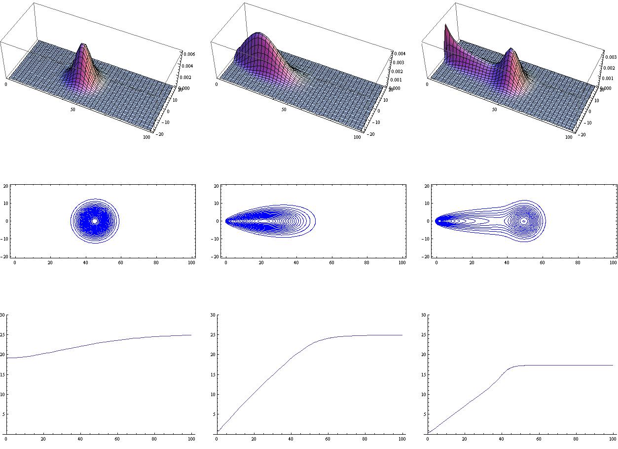
Proposition 5.2 seems to suggest that the strange phenomenon in the conditional variance (not increasing as in Figure 1) will disappear if we consider independent increments $(X_{k},Y_{k})$ where $X_{k}$ is also independent of $Y_{k}$ for $k=1,2,\cdots,K_{n}$. However, we will give a mean zero nearest neighbor random walk example, where this phenomenon is still present.

Let $(X_{k},Y_{k}),k\geq 1$ be independent identical distributed random vectors with distribution

$$\begin{split}{\rm P}\left((X_{k},Y_{k})=(1,\pm 1)\right)={\rm P}\left((X_{k},Y_{k})=(-1,\pm 1)\right)=\xi,\quad{\rm P}\left((X_{k},Y_{k})=(\pm 1,0)\right)=\frac{1}{2}-2\xi.\end{split}$$

where $0<\xi<1/4$. Obviously, $X_{k}$ is independent of $Y_{k}$. Let $\bar{S}(n)=(\bar{S}_{X}(n),\bar{S}_{Y}(n))$ be the position of the particle at time $n$. One can compute its probability mass function and conditional variance ${\rm Var}\left(\bar{S}_{Y}(n)~{}|~{}\bar{S}_{X}(n)=x\right)$.

Example 5.2.

Let $n=25,a=b=0.01,\xi=0.2$, and $\nu=\pi$. See Figure 3.

Figure 3. The probability mass function of $\bar{S}(25)$, a list contour plot of its mass function and the conditional variance ${\rm Var}\left(\bar{S}_{Y}(25)~{}|~{}\bar{S}_{X}(25)=2x\right)$ with $\nu=\pi,a=b=0.01,\;\xi=0.2$.

6. Gaussian dispersion

It is natural (and common practice in the engineering literature, see e.g., [3]) to consider a Gaussian dispersion. Let $\mathbf{S}(n)$ be the position of the particle at time $n$ as described in Section 2 except that $(X_{k},Y_{k})$ now has a Gaussian distribution with independent marginals

$$X_{k}\stackrel{{\scriptstyle\mathbf{d}}}{{=}}\mathcal{N}(0,2\alpha),\quad Y_{k}\stackrel{{\scriptstyle\mathbf{d}}}{{=}}\mathcal{N}(0,2\beta)\quad\textrm{for}~{}\alpha,\beta>0.$$

Proposition 6.1.

For $n\geq 1$, the distribution $\mu_{n}$ of the random variable $\mathbf{S}(n)$ can be written as

$$\mu_{n}=f_{n}(0)\delta_{(0,0)}+(1-f_{n}(0))\tilde{\mu}_{n},$$

where $\delta_{(0,0)}$ is Dirac measure at the point $(0,0)$ and $\tilde{\mu}_{n}$ is the distribution of a continuous random variable having density function

$$\tilde{f}_{\mathbf{S}(n)}(x,y)=\frac{1}{1-f_{n}(0)}\sum_{k=1}^{n}\frac{f_{n}(k)}{4\pi k\sqrt{\alpha\beta}}\exp{\Big{(}-\frac{(x-k)^{2}}{4k\alpha}-\frac{y^{2}}{4k\beta}\Big{)}}.$$

Moreover, the conditional variance is given by

$${\rm Var}\left(\mathbf{S}_{Y}(n)~{}|~{}\mathbf{S}_{X}(n)=x\right)=2\beta(1-f_{n}(0))\frac{\sum_{k=1}^{n}\exp{\big{(}-(x-k)^{2}/(4k\alpha)\big{)}}f_{n}(k)\sqrt{k}}{\sum_{k=1}^{n}\exp{\big{(}-(x-k)^{2}/(4k\alpha)\big{)}}f_{n}(k)/\sqrt{k}}.$$

Proof.

As in [2] one easily finds the characteristic function $\varphi_{\mathbf{S}(n)}$ of $\mathbf{S}(n)$, and as in [2] one shows that $(0,0)$ is the unique atom of $\mu_{n}$, with mass $f_{n}(0)$. Then the density function of the continuous part of $\mu_{n}$ follows by inverse Fourier transformation:

$$\begin{split}\tilde{f}_{\mathbf{S}(n)}(x,y)&=\frac{1}{1-f_{n}(0)}\frac{1}{(2\pi)^{2}}\int\int\big{(}\varphi_{\mathbf{S}(n)}(u_{1},u_{2})-f_{n}(0)\big{)}\mathrm{e}^{-i(u_{1}x+u_{2}y)}\mathrm{d}u_{1}\mathrm{d}u_{2}\\ &=\frac{1}{1-f_{n}(0)}\sum_{k=1}^{n}f_{n}(k)\frac{1}{(2\pi)^{2}}\int\int\mathrm{e}^{-iu_{1}x+k(iu_{1}-\alpha u_{1}^{2})}\mathrm{e}^{-iu_{2}y-k\beta u_{2}^{2}}\mathrm{d}u_{1}\mathrm{d}u_{2}\\ &=\frac{1}{1-f_{n}(0)}\sum_{k=1}^{n}f_{n}(k)\frac{1}{4\pi k\sqrt{\alpha\beta}}\exp{\Big{(}-\frac{(x-k)^{2}}{4k\alpha}-\frac{y^{2}}{4k\beta}\Big{)}}.\end{split}$$

Using symmetry, the conditional variance is given by

$$\begin{split}{\rm Var}\left(\mathbf{S}_{Y}(n)~{}|~{}\mathbf{S}_{X}(n)=x\right)={\rm E}\left(\mathbf{S}_{Y}^{2}(n)~{}|~{}\mathbf{S}_{X}(n)=x\right)=(1-f_{n}(0))\int_{-\infty}^{\infty}y^{2}\frac{\tilde{f}_{\mathbf{S}(n)}(x,y)}{\tilde{f}_{\mathbf{S}_{X}(n)}(x)}\mathrm{d}y,\end{split}$$

where $\tilde{f}_{\mathbf{S}_{X}(n)}(x)=\int_{-\infty}^{\infty}\tilde{f}_{\mathbf{S}(n)}(x,y)\mathrm{d}y.$ The proof is then finished by a straightforward calculation. ∎

Example 6.1.

Let $n=50,\alpha=\beta=1/4$, and the initial distribution $\nu=\pi$. See Figure 4.

Figure 4. The density $\tilde{f}_{\mathbf{S}(50)}$, a contour plot of the density and the conditional variance ${\rm Var}\left(\mathbf{S}_{Y}(50)~{}|~{}\mathbf{S}_{X}(50)=x\right)$ with $\nu=\pi,\alpha=\beta=1/4$. In the first column $a=0.1,b=0.9$; in the second column $a=b=0.1$; in the last column $a=b=0.01$.

Figure 4 suggests that the conditional variance ${\rm Var}\left(\mathbf{S}_{Y}(n)~{}|~{}\mathbf{S}_{X}(n)=x\right)$ is increasing in $x$. This is indeed the case, and is the content of the following proposition.

Proposition 6.2.

The conditional variance ${\rm Var}\left(\mathbf{S}_{Y}(n)~{}|~{}\mathbf{S}_{X}(n)=x\right)$ is an increasing function in $x$.

Proof.

Since by Proposition 6.1 ${\rm Var}\left(\mathbf{S}_{Y}(n)~{}|~{}\mathbf{S}_{X}(n)=x\right)$ is a differentiable function, we only need to show that its first derivative is nonnegative. For simplicity, we write for

$$g(x)=\sum_{k=1}^{n}f_{n}(k)\sqrt{k}\mathrm{e}^{-\frac{(x-k)^{2}}{4k\alpha}},\quad h(x)=\sum_{k=1}^{n}\frac{f_{n}(k)}{\sqrt{k}}\mathrm{e}^{-\frac{(x-k)^{2}}{4k\alpha}}.$$

So ${\rm Var}\left(\mathbf{S}_{Y}(n)~{}|~{}\mathbf{S}_{X}(n)=x\right)^{\prime}=\frac{2\beta(1-f_{n}(0))}{h^{2}(x)}\big{(}g^{\prime}(x)h(x)-g(x)h^{\prime}(x)\big{)}$. Note that

$$\begin{split}&g^{\prime}(x)h(x)-g(x)h^{\prime}(x)\\ =&~{}\frac{1}{2\alpha}\sum_{k,\ell=1}^{n}\frac{f_{n}(k)}{\sqrt{k}}\frac{f_{n}(\ell)}{\sqrt{\ell}}\mathrm{e}^{-\frac{(x-k)^{2}}{4k\alpha}-\frac{(x-\ell)^{2}}{4\ell\alpha}}\frac{\ell-k}{k}(x-k)\\ =:&~{}\frac{1}{2\alpha}\sum_{k,\ell=1}^{n}w(k,\ell)\frac{\ell-k}{k}(x-k),\end{split}$$

where $w(k,\ell)=\frac{f_{n}(k)}{\sqrt{k}}\frac{f_{n}(\ell)}{\sqrt{\ell}}\mathrm{e}^{-\frac{(x-k)^{2}}{4k\alpha}-\frac{(x-\ell)^{2}}{4\ell\alpha}}\geq 0$. Using the symmetry $w(k,\ell)=w(\ell,k)$, the proposition then follows from

$$\begin{split}&g^{\prime}(x)h(x)-g(x)h^{\prime}(x)\\ =&~{}\frac{1}{4\alpha}\Big{[}\sum_{k,\ell=1}^{n}w(k,\ell)\frac{\ell-k}{k}(x-k)+\sum_{k,\ell=1}^{n}w(\ell,k)\frac{k-\ell}{\ell}(x-\ell)\Big{]}\\ =&~{}\frac{1}{4\alpha}\sum_{k,\ell=1}^{n}w(k,\ell)(\ell-k)\big{[}(\frac{x}{k}-1)-(\frac{x}{\ell}-1)\big{]}=\frac{x}{4\alpha}\sum_{k,\ell=1}^{n}w(k,\ell)\frac{(\ell-k)^{2}}{k\ell}~{}\geq 0.\end{split}$$

∎

References

- [1] Michel Dekking and DeRong Kong. Multimodality of the Markov binomial distribution. Journal of Applied Probability, 48(4):938–953, 2011.
- [2] Michel Dekking and DeRong Kong. A simple stochastic kinetic transport model. arXiv: 1106.2912v1, to appear in Advances in Applied Probability, 2012.
- [3] A.M. Michalak and Peter K. Kitanidis. Macroscopic behavior and random-walk particle tracking of kinetically sorbing solutes. Water Resources Research, 36(8):2133–2146, 2000.
- [4] E. Omey, J. Santos, and S. Van Gulck. A Markov-binomial distribution. Appl. Anal. Discrete Math., 2(1):38–50, 2008.
- [5] G. Uffink, A. Elfeki, F.M. Dekking, J. Bruining, and C. Kraaikamp. Understanding the non-gaussianity of reactive transport; from particle dynamics to PDE’s. Transp Porous Med, pages 1–25, 2011.