Analysis of Resonant Inelastic X-Ray Scattering in Stripe-Ordered Nickelate

Abstract

We analyze theoretically the resonant inelastic x-ray scattering (RIXS) at the Ni $K$ edge in the stripe-ordered state of La_2-xSr_xNiO₄ at $x=1/3$. In the calculation of RIXS spectra, the stripe-ordered ground state is described within the Hartree-Fock approximation by using a realistic tight-binding model for Ni3$d\gamma$ and O2$p_{x,y}$ orbitals, and the electron correlations in the electronic excitation processes are taken into account within the random-phase approximation. The calculated RIXS spectrum shows a tail toward the low-energy region when the momentum transfer of photons equals the stripe vector ${\mib Q}$, being consistent with a recent experimental result. The origin of this anomalous momentum dependence of RIXS spectra is discussed microscopically.

1 Introduction

Resonant inelastic x-ray scattering (RIXS) has been developed to be a powerful method for measuring elementary excitations in solids [1, 2, 3]. This is largely owing to both the recent advances in instrumentations and the achievement of highly brilliant lights obtained from advanced synchrotron facilities. In RIXS processes, the incident photon energy is tuned to match an absorption energy of one of the constituent elements. The electronic system of materials is resonantly excited by absorbing incident photons, and then after a short time (typically, of the order of femtoseconds), photons are emitted, whose momentum and energy generally differ from those of the incident photons. The electronic system remains an excited state still after the photon is emitted. The momentum change and energy loss of photons necessarily equal the momentum and energy spent for exciting the electronic system, due to the energy and momentum conservation laws. Therefore, one can get information on the electronic excitations of the system by measuring systematically the momentum change and energy loss of photons.

Excitation processes involved in RIXS depend on the material and incident x-ray wavenumber utilized in the RIXS measurements. Among them, RIXS at the transition-metal $K$ edges has attracted much interest, partly because the RIXS spectra are naturally expected to reflect the strong electron correlations of $d$ electrons in transition-metal compounds, such as cuprates [4, 5, 6, 7, 8, 9, 10, 11, 12, 13, 14, 15, 16], manganites [17, 18], nickelates [19, 15] etc. In the RIXS at the transition-metal $K$ edges, transition-metal $1s$ core electrons are resonantly excited to the transition-metal $4p$ unoccupied bands. In the intermediate states, the transition-metal $d$ electrons are excited to screen the created $1s$ core hole. Here we should note that the core hole potential, i.e., the Coulomb interaction between the transition-metal $1s$ and $d$ orbitals, plays an essential role. In the final state, the $4p$ electron is annihilated together with the $1s$ hole by emitting a photon, before the $d$ electrons decay from the excited state to the ground state. Overall, the momentum change and energy loss of photons are transferred indirectly to the excited $d$ electrons.

The x-ray at the transition-metal $K$ edges is situated in the hard x-ray regime, and its wavenumber is appropriate for sweeping the whole Brillouin zone. Taking advantage of this point, momentum dependence of the RIXS spectra has been indeed observed in various transition-metal compounds, such as copper oxides [6, 8, 7, 9, 10, 11, 12, 13, 15, 16], NiO [20] etc. As a recent result from intensive experimental and theoretical researches, it has now become clear that the RIXS spectra at the transition-metal $K$ edges reflect the charge correlation function of the strongly correlated $d$ electrons [21, 22, 23, 24, 11, 26, 25]. As well known, neutron scattering intensity is related to the spin correlation function. Thus, roughly speaking, RIXS in transition-metal compounds is to charge correlations what neutron scattering is to spin correlations. According to more recent researches, multi-magnon excitations have been observed at low-energy regions in insulating cuprates [27, 28]. Therefore RIXS may provide a promising way of studying not only charge excitations but also magnetic excitations of strongly correlated electrons in transition-metal compounds in the future.

Stripe ordering has been one of the central issues in the physics of strongly correlated electron systems. Neutron scattering measurements have revealed that the holes and spins exhibit spatial disproportionation with a stripe form in several transition-metal oxides, e.g., La_2-xSr_xNiO₄ [29, 30, 31, 32], La₂NiO_4+δ [33, 34], La_2-x(Ba, Sr)_xCuO₄ at $x=\frac{1}{8}$ [35], etc. To try to elucidate relations to the high-$T_{\rm c}$ cuprate superconductivity, a lot of research works on stripe ordering have already been accumulated so far [36]. Recently, Wakimoto and collaborators reported RIXS in two stripe-ordered 214 compounds La_5/3Sr_1/3NiO₄ and $1/8$ doped La_2-x(Ba or Sr)_xCuO₄ at the Cu and Ni $K$ edges, respectively [37]. They observed low-energy ($\simeq$ 1 eV) excitations with a momentum transfer corresponding to the charge stripe spatial period in the both compounds. The aim of our present work is to analyze this anomalous spectral feature, and discuss its microscopic origin for the case of La_5/3Sr_1/3NiO₄.

The present article is constructed as follows. In § 2, we present a model Hamiltonian, theoretical description of the stripe-ordered state, and the formula for RIXS intensity. We take the Hartree-Fock (HF) approximation for describing the stripe-ordered ground states, and the random-phase approximation (RPA) for taking account of the electron correlations in the intermediate states of the excitation processes. In § 3, numerical results of RIXS spectra are presented. There we present not only the results for stripe states (§ 3.2) but also for the undoped antiferromagnetic insulating state (§ 3.1). In § 4, the article is concluded with some discussions and remarks.

2 Formulation

2.1 Model and Hartree-Fock approximation for stripe states

The electronic properties of La_2-xSr_xNiO₄ are considered to be dominated by those of the NiO₂ layers. Therefore we can use two-dimensional tight-binding model for a single NiO layer to reproduce the in-plane electronic structure of La_2-xSr_xNiO₄. Since only Ni$3d\gamma$ orbitals are the most essential among the five Ni$3d$ orbitals, we take the following four orbitals: Ni$3d_{x^{2}-y^{2}}$, Ni$3d_{3z^{2}-r^{2}}$, O2$p_{x}$ and O$2p_{y}$. Hereafter, we specify each of these four orbitals by index $\ell$: $\ell=1$ for Ni$3d_{x^{2}-y^{2}}$, $\ell=2$ for Ni$3d_{3z^{2}-r^{2}}$, $\ell=3$ for O$2p_{x}$, $\ell=4$ for O$2p_{y}$. The noninteracting part of the Hamiltonian is given by

$$H_{0}=\sum_{i}\sum_{\ell\sigma}\varepsilon_{\ell}c^{{\dagger}}_{i\ell\sigma}c_{i\ell\sigma}+\sum_{i,j}\sum_{\ell\ell^{\prime}\sigma}t_{\ell,\ell^{\prime}}({\mib r}_{ij})c^{{\dagger}}_{i\ell\sigma}c_{j\ell^{\prime}\sigma},$$ (1)

where ${\mib r}_{ij}={\mib r}_{i}-{\mib r}_{j}$, $\ell$ and $\ell^{\prime}$ are orbital indices, $c_{i\ell\sigma}$ and $c^{{\dagger}}_{i\ell\sigma}$ are respectively the annihilation and creation operators for the electron with spin $\sigma$ on orbital $\ell$ at site $i$.

For the one-particle energies, we take $\varepsilon_{1}=\varepsilon_{2}\equiv\varepsilon_{d}=-9$ eV, $\varepsilon_{3}=\varepsilon_{4}\equiv\varepsilon_{p}=0$ eV. For the hopping parameters we take $t_{1,3}(\frac{\hat{x}}{2})=-t_{1,4}(\frac{\hat{y}}{2})\equiv t_{dp}=-1.2$ eV and $t_{2,3}(\frac{\hat{x}}{2})=t_{2,4}(\frac{\hat{y}}{2})\equiv-t_{dp}/\sqrt{3}$ for nearest-neighbor Ni-O bonds, $t_{3,4}(\frac{\hat{x}+\hat{y}}{2})=-t_{3,4}(\frac{\hat{x}-\hat{y}}{2})\equiv t_{pp}=0.6$ eV for nearest-neighbor O-O bonds. ($\hat{x}$ and $\hat{y}$ are the unit lattice vectors connecting inplane nearest-neighbor Ni sites.) The hopping matrix $t_{\ell,\ell^{\prime}}({\mib r})$ satisfies the relation $t_{\ell,\ell^{\prime}}({\mib r})=t_{\ell^{\prime},\ell}(-{\mib r})=s_{\ell}s_{\ell^{\prime}}t_{\ell,\ell^{\prime}}(-{\mib r})$, where the factor $s_{\ell}$ equals $+1$ for $\ell=1$ and $2$ (Ni$3d$ orbitals), and $-1$ for $\ell=3$ and $4$ (O$2p$ orbitals). The Fourier transform of the above non-interacting Hamiltonian is given in the following form:

$$H_{0}=\sum_{{\mib k}}\sum_{\ell\ell^{\prime}}\sum_{\sigma}\xi_{\ell\ell^{\prime}}({\mib k})c^{{\dagger}}_{{\mib k}\ell\sigma}c_{{\mib k}\ell^{\prime}\sigma},$$ (2)

with

$$\xi_{\ell\ell^{\prime}}({\mib k})=\varepsilon_{\ell}\delta_{\ell\ell^{\prime}}+\sum_{\mib r}e^{-{\rm i}{\mib k}\cdot{\mib r}}t_{\ell,\ell^{\prime}}({\mib r}),$$ (3)

where ${\mib k}$ denotes momentum in the first Brillouin zone (BZ). For the convenience in the following, we introduce the annihilation operators $d$ and $p$ [creation operators $d^{{\dagger}}$ and $p^{{\dagger}}$] by $(d_{i1\sigma},d_{i2\sigma},p_{i3\sigma},p_{i4\sigma})\equiv(c_{i1\sigma},c_{i2\sigma},c_{i3\sigma},c_{i4\sigma})$ [ $(d_{i1\sigma}^{{\dagger}},d_{i2\sigma}^{{\dagger}},p_{i3\sigma}^{{\dagger}},p_{i4\sigma}^{{\dagger}})\equiv(c_{i1\sigma}^{{\dagger}},c_{i2\sigma}^{{\dagger}},c_{i3\sigma}^{{\dagger}},c_{i4\sigma}^{{\dagger}})$ ]. Namely, $d_{i\ell\sigma}\equiv c_{i\ell\sigma}$ when $i$ is on Ni site and $\ell=1$ or $2$, and $p_{i\ell\sigma}\equiv c_{i\ell\sigma}$ when $i$ is on O site and $\ell=3$ or $4$. For the momentum representation, we have $d_{{\mib k}\ell\sigma}\equiv c_{{\mib k}\ell\sigma}$ for $\ell=1$ and $2$, and $p_{{\mib k}\ell\sigma}\equiv c_{{\mib k}\ell\sigma}$ for $\ell=3$ and $4$.

For the interacting part, we take the on-site Coulomb interaction at Ni sites:

$$H^{\prime} = \frac{U}{2}\sum_{i}\sum_{\ell}\sum_{\sigma\neq\sigma^{\prime}}d_{i\ell\sigma}^{{\dagger}}d_{i\ell\sigma^{\prime}}^{{\dagger}}d_{i\ell\sigma^{\prime}}d_{i\ell\sigma}$$ (4)

$$+\frac{U^{\prime}}{2}\sum_{i}\sum_{\ell\neq\ell^{\prime}}\sum_{\sigma,\sigma^{\prime}}d_{i\ell\sigma}^{{\dagger}}d_{i\ell^{\prime}\sigma^{\prime}}^{{\dagger}}d_{i\ell^{\prime}\sigma^{\prime}}d_{i\ell\sigma}$$

$$+\frac{J}{2}\sum_{i}\sum_{\ell\neq\ell^{\prime}}\sum_{\sigma,\sigma^{\prime}}d_{i\ell\sigma}^{{\dagger}}d_{i\ell^{\prime}\sigma^{\prime}}^{{\dagger}}d_{i\ell\sigma^{\prime}}d_{i\ell^{\prime}\sigma}$$

$$+\frac{J^{\prime}}{2}\sum_{i}\sum_{\ell\neq\ell^{\prime}}\sum_{\sigma\neq\sigma^{\prime}}d_{i\ell\sigma}^{{\dagger}}d_{i\ell\sigma^{\prime}}^{{\dagger}}d_{i\ell^{\prime}\sigma^{\prime}}d_{i\ell^{\prime}\sigma},$$

where $i$ is on Ni sites, $\ell$ and $\ell^{\prime}$ are 1 or 2. $U$ is the intra-orbital Coulomb repulsion, $U^{\prime}$ is the inter-orbital Coulomb repulsion, $J$ is the Hund’s rule coupling and $J^{\prime}$ is the inter-orbital pair-hopping term. Throughout the present study, we take $U=8$ eV, $U^{\prime}=6$ eV, and $J=J^{\prime}=1$ eV.

To deal with the many-body problem originating from $H^{\prime}$, we adopt the HF approximation. A lot of HF calculations using Hubbard-type models have been performed to study stripe ordering, so far [38, 39, 40, 41, 42, 43, 44, 45, 46, 47]. Here we introduce the mean fields

$$\langle d_{i\ell\sigma}^{{\dagger}}d_{i\ell\sigma}\rangle=\frac{1}{2}(n_{i\ell}+m_{i\ell}\sigma),$$ (5)

where the $n_{i\ell}$ and $m_{i\ell}$ are the electron number and the spin magnetic moment in orbital $\ell$ at Ni site $i$, respectively. We assume that the stripe ordering characterized by stripe vectors ${\mib Q}$’s is realized. In this case, the mean fields are expressed in the form:

$$n_{i\ell} = \sum_{\mib Q}e^{{\rm i}{\mib Q}\cdot{\mib r}_{i}}n_{{\mib Q}\ell},$$ (6)

$$m_{i\ell} = \sum_{\mib Q}e^{{\rm i}{\mib Q}\cdot{\mib r}_{i}}m_{{\mib Q}\ell},$$ (7)

where $i$ is on Ni sites and $\ell$ is for Ni3$d$ orbitals, and ${\mib Q}$’s characterize the spatial periodicity of the stripe. In the present study, we restrict ourselves to diagonal stripe ordering expected from experimental results for La_5/3Sr_1/3NiO₄ and the above summation in ${\mib Q}$ is performed for ${\mib Q}=n\cdot{\mib Q}_{s}$ $(n=0,1,2)$, where ${\mib Q}_{s}=(\frac{2}{3}\pi,\frac{2}{3}\pi)$. $n_{{\mib Q}\ell}=n_{-{\mib Q}\ell}^{*}$ and $m_{{\mib Q}\ell}=m_{-{\mib Q}\ell}^{*}$ hold, since $n_{i\ell}$ and $m_{i\ell}$ are real quantities. As a result of the HF approximation, the total mean-field Hamiltonian $H_{\rm MF}=H_{0}+H_{\rm MF}^{\prime}$ is given in the form:

$$H_{MF}=\sum_{{\mib k}}\sum_{\ell\ell^{\prime}\sigma}\xi_{\ell\ell^{\prime}}({\mib k})c^{{\dagger}}_{{\mib k}\ell\sigma}c_{{\mib k}\ell^{\prime}\sigma}+\sum_{{\mib k}}\sum_{\mib Q}\sum_{\ell\sigma}\Delta_{{\mib Q}\ell\sigma}d^{{\dagger}}_{{\mib k}\ell\sigma}d_{{\mib k}-{\mib Q}\ell\sigma}+E_{0},$$ (8)

with

$$\Delta_{{\mib Q}\ell\sigma} = \frac{U}{2}(n_{{\mib Q}\ell}-m_{{\mib Q}\ell}\sigma)+U^{\prime}\sum_{\ell^{\prime}(\neq\ell)}n_{{\mib Q}\ell^{\prime}}$$ (9)

$$-\frac{J}{2}\sum_{\ell^{\prime}(\neq\ell)}(n_{{\mib Q}\ell^{\prime}}+m_{{\mib Q}\ell^{\prime}}\sigma),$$

$$E_{0} = -\frac{NU}{4}\sum_{\mib Q}\sum_{\ell}(|n_{{\mib Q}\ell}|^{2}-|m_{{\mib Q}\ell}|^{2})-\frac{NU^{\prime}}{2}\sum_{\mib Q}\sum_{\ell\neq\ell^{\prime}}n_{{\mib Q}\ell}n_{{\mib Q}\ell^{\prime}}^{*}$$ (10)

$$+\frac{NJ}{4}\sum_{\mib Q}\sum_{\ell\neq\ell^{\prime}}(n_{{\mib Q}\ell}n_{{\mib Q}\ell^{\prime}}^{*}+m_{{\mib Q}\ell}m_{{\mib Q}\ell^{\prime}}^{*}).$$

The first BZ is folded, since the spatial periodicity of the charge disproportionation is integer times of the original lattice periodicity. We express momentum ${\mib k}$ in the original BZ by using the stripe vector ${\mib Q}$ and reduced momentum ${\mib k}_{0}$ as ${\mib k}={\mib k}_{0}+{\mib Q}$, where ${\mib k}_{0}$ is restricted in the folded BZ. In the present study, we use the reduced BZ depicted in Fig. 1, to solve the HF equation for the stripe-ordered states with ${\mib Q}_{s}=(\frac{2}{3}\pi,\frac{2}{3}\pi)$. Thus the total mean-field Hamiltonian is expressed in the form:

$$H_{MF} = \sum_{{\mib k}_{0}}\sum_{{\mib Q}}\sum_{\ell\ell^{\prime}\sigma}\xi_{\ell\ell^{\prime}}({\mib k}_{0}+{\mib Q})c^{{\dagger}}_{{{\mib k}_{0}+\mib Q}\ell\sigma}c_{{\mib k}_{0}+{\mib Q}\ell^{\prime}\sigma}$$ (11)

$$+\sum_{{\mib k}_{0}}\sum_{{\mib Q},{\mib Q}^{\prime}}\sum_{\ell\sigma}\Delta_{{\mib Q}-{\mib Q}^{\prime}\ell\sigma}d^{{\dagger}}_{{\mib k}_{0}+{\mib Q}\ell\sigma}d_{{\mib k}_{0}+{\mib Q}^{\prime}\ell\sigma}+E_{0}.$$

We should note that the summation in momentum ${\mib k}_{0}$ is restricted only over the reduced BZ. By diagonalizing this mean-field Hamiltonian, we have the energy dispersions $E_{a,\sigma}({\mib k}_{0})$ and unitary matrix $U_{{\mib Q},\ell,a,\sigma}({\mib k}_{0})$ for diagonalization, where $a$ is the index for the diagonalized bands. The self-consistency condition for mean fields is given by

$$n_{{\mib Q}\ell} = \frac{1}{N}\sum_{{\mib k}_{0}}\sum_{{\mib Q}^{\prime}}\sum_{a,\sigma}U_{{\mib Q}^{\prime},\ell,a,\sigma}^{*}({\mib k}_{0})U_{{\mib Q}^{\prime}+{\mib Q},\ell,a,\sigma}({\mib k}_{0})n_{a,\sigma}({\mib k}_{0}),$$ (12)

$$m_{{\mib Q}\ell} = \frac{1}{N}\sum_{{\mib k}_{0}}\sum_{{\mib Q}^{\prime}}\sum_{a,\sigma}\sigma U_{{\mib Q}^{\prime},\ell,a,\sigma}^{*}({\mib k}_{0})U_{{\mib Q}^{\prime}+{\mib Q},\ell,a,\sigma}({\mib k}_{0})n_{a,\sigma}({\mib k}_{0}),$$ (13)

where $n_{a,\sigma}({\mib k}_{0})$ is the electron occupation number on band $a$ at momentum ${\mib k}_{0}$ with spin $\sigma$: $n_{a,\sigma}({\mib k}_{0})=f(E_{a,\sigma}({\mib k}_{0}))$ ($f(E)$ is the Fermi distribution function).

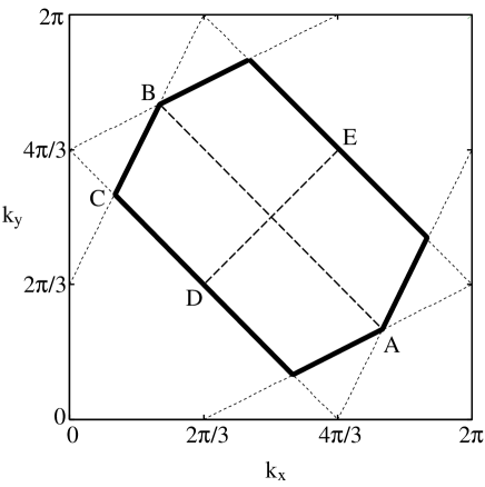
Figure 1: A typical reduced BZ for the diagonal stripe state is enclosed by the thick solid line. The wave vectors at some symmetry points are also indicated: A$(\frac{14}{9}\pi,\frac{4}{9}\pi)$, B$(\frac{4}{9}\pi,\frac{14}{9}\pi)$, C$(\frac{2}{9}\pi,\frac{10}{9}\pi)$, D$(\frac{2}{3}\pi,\frac{2}{3}\pi)$, E$(\frac{4}{3}\pi,\frac{4}{3}\pi)$.

Here we take account of the electron-lattice interaction, since it is natural to consider that lattice distortions occur cooperatively with the charge disproportionation accompanying the stripe ordering, as discussed in refs. References, References and References. We denote the atom displacement at site $i$ by ${\mib u}({\mib r}_{i})$. If we assume $t_{\ell,\ell^{\prime}}({\mib r})\propto|{\mib r}|^{-\alpha_{\ell\ell^{\prime}}}$ ($\alpha_{\ell\ell^{\prime}}=\alpha_{\ell^{\prime}\ell}$), the change of the hopping parameters due to the atom displacement is evaluated approximately by $\delta t_{\ell,\ell^{\prime}}({\mib r}_{ij})=-\alpha_{\ell\ell^{\prime}}t_{\ell,\ell^{\prime}}({\mib r}_{ij})\frac{{\mib r}_{ij}\cdot{\mib u}_{ij}}{|{\mib r}_{ij}|^{2}}$, where ${\mib u}_{ij}={\mib u}({\mib r}_{i})-{\mib u}({\mib r}_{j})$. Hereafter, for ${\mib u}_{ij}$ and ${\mib r}_{ij}$, we use units normalized by the lattice constant. The modification to the Hamiltonian $H_{0}$ due to the lattice distortions is given by

$$H_{\rm l.d.}=\sum_{i,j}\sum_{\ell\ell^{\prime}\sigma}\Bigl{[}-\alpha_{\ell\ell^{\prime}}t_{\ell,\ell^{\prime}}({\mib r}_{ij})\frac{{\mib r}_{ij}\cdot{\mib u}_{ij}}{|{\mib r}_{ij}|^{2}}\Bigr{]}c^{{\dagger}}_{i\ell\sigma}c_{j\ell^{\prime}\sigma}.$$ (14)

Throughout the present study, we take $\alpha_{\ell\ell^{\prime}}\equiv\alpha_{dp}=3.5$ for $(\ell,\ell^{\prime})=(1$ or $2,3$ or $4)$, $(3$ or $4,1$ or $2)$ (Ni-O bonds), and $\alpha_{\ell\ell^{\prime}}\equiv\alpha_{pp}=2$ for $(\ell,\ell^{\prime})=(3$ or $4,3$ or $4)$ (O-O bonds) [48]. We use the following form for the lattice elastic energy,

$$E_{\rm L}[{\mib u}_{ij}]=\frac{1}{2}\sum_{(i,j)}K_{A_{i},A_{j}}(|{\mib r}_{ij}|)|{\mib u}_{ij}|^{2},$$ (15)

where $A_{i}$ and $A_{j}$ denote the atoms (Ni or O) at sites $i$ and $j$, respectively, and $K_{A_{i},A_{j}}(|{\mib r}_{ij}|)$ is the elastic constant of the bond between atoms $A_{i}$ and $A_{j}$. The summation with $(i,j)$ means that with respect to all pairs of sites. Minimizing the total energy

$$E_{\rm tot}=\langle H_{0}+H^{\prime}+H_{\rm l.d.}+E_{\rm L}\rangle$$ (16)

with respect to the lattice distortion ${\mib u}_{ij}$ and using the Hellmann-Feynman theorem, we have the following equation for determining ${\mib u}_{ij}$:

$${\mib u}_{ij}=\frac{1}{K_{A_{i},A_{j}}(|{\mib r_{ij}}|)}\sum_{\ell\ell^{\prime}\sigma}\alpha_{\ell\ell^{\prime}}t_{\ell,\ell^{\prime}}({\mib r}_{ij})\frac{{\mib r}_{ij}}{|{\mib r}_{ij}|^{2}}\langle c_{i\ell\sigma}^{{\dagger}}c_{j\ell^{\prime}\sigma}+c_{j\ell^{\prime}\sigma}^{{\dagger}}c_{i\ell\sigma}\rangle,$$ (17)

where the summation in $\ell$ ($\ell^{\prime}$) is restricted to the orbitals on atom $A_{i}$ ($A_{j}$) at site $i$ ($j$). As can be seen easily, this condition eq. (17) is not effective for pairs of sites $i$ and $j$ for which $t_{\ell,\ell^{\prime}}({\mib r}_{ij})$ equals zero for any choice of $\ell$ and $\ell^{\prime}$. In the present study, since we take only hoppings for nearest-neighbor Ni$3d$-O$2p$ and O$2p$-O$2p$ bonds, only ${\mib u}_{ij}$’s for these bonds are determined by eq. (17), while ${\mib u}_{ij}$’s for the other bonds are not.

Here we assume that the lattice distortions possess the same spatial periodicity as the stripe order, and then can expand ${\mib u}_{ij}$ in the form

$${\mib u}_{ij}=\sum_{{\mib Q},{\mib Q}^{\prime}}{\mib u}_{{\mib Q}\ell,{\mib Q}^{\prime}\ell^{\prime}}({\mib r}_{ij})e^{{\rm i}({\mib Q}\cdot{\mib r}_{i}-{\mib Q}^{\prime}\cdot{\mib r}_{j})},$$ (18)

where $\ell$ and $\ell^{\prime}$ denote the atomic orbitals at sites $i$ and $j$, respectively. $H_{\rm l.d.}$ is expressed in the momentum representation as

$$H_{\rm l.d.}=\sum_{{\mib k}_{0}}\sum_{{\mib Q},{\mib Q}^{\prime}}\sum_{\ell\ell^{\prime}\sigma}\eta_{\ell\ell^{\prime}}({\mib k}_{0};{\mib Q},{\mib Q}^{\prime})c_{{\mib k}_{0}+{\mib Q}\ell\sigma}^{\dagger}c_{{\mib k}_{0}+{\mib Q}^{\prime}\ell^{\prime}\sigma},$$ (19)

with

$$\eta_{\ell\ell^{\prime}}({\mib k}_{0};{\mib Q},{\mib Q}^{\prime})=-\alpha_{\ell\ell^{\prime}}\sum_{\mib r}t_{\ell,\ell^{\prime}}({\mib r})\frac{e^{-{\rm i}{\mib k}_{0}\cdot{\mib r}}}{|{\mib r}|^{2}}\sum_{{\mib Q}^{\prime\prime}}[{\mib r}\cdot{\mib u}_{{{\mib Q}-{\mib Q}^{\prime\prime}}\ell,{{\mib Q}^{\prime}-{\mib Q}^{\prime\prime}}\ell^{\prime}}({\mib r})]e^{-{\rm i}{\mib Q}^{\prime\prime}\cdot{\mib r}}.$$ (20)

The energy minimization condition eq. (17) is given in the momentum representation by

$${\mib u}_{{\mib Q}\ell,{\mib Q}^{\prime}\ell^{\prime}}({\mib r}_{ij})=\frac{1}{K_{A_{i},A_{j}}(|{\mib r}_{ij}|)}\sum_{mm^{\prime}}\alpha_{mm^{\prime}}t_{m,m^{\prime}}({\mib r}_{ij})\frac{{\mib r}_{ij}}{|{\mib r}_{ij}|^{2}}$$

$$\times\frac{1}{N}\sum_{{\mib k}_{0}}\sum_{a\sigma}[e^{-{\rm i}{\mib k}_{0}\cdot{\mib r}_{ij}}U_{-{\mib Q},m,a,\sigma}^{*}({\mib k}_{0})U_{-{\mib Q}^{\prime},m^{\prime},a,\sigma}({\mib k}_{0})$$

$$+e^{{\rm i}{\mib k}_{0}\cdot{\mib r}_{ij}}U_{{\mib Q}^{\prime},m^{\prime},a,\sigma}^{*}({\mib k}_{0})U_{{\mib Q},m,a,\sigma}({\mib k}_{0})]n_{a,\sigma}({\mib k}_{0}),$$ (21)

where $A_{i}$ and $A_{j}$ denote atoms on which orbitals $\ell$ and $\ell^{\prime}$ are, respectively, and the summation in $m$ and $m^{\prime}$ is restricted to the orbitals on the atoms $A_{i}$ and $A_{j}$, respectively. $U_{{\mib Q},\ell,a,\sigma}({\mib k}_{0})$ is the diagonalization matrix for $H_{\rm MF}+H_{\rm l.d.}$. As easily seen, ${\mib u}_{{\mib Q}\ell,{\mib Q}^{\prime}\ell^{\prime}}({\mib r}_{ij})$ satisfies the following equalities,

$${\mib u}_{{\mib Q}\ell,{\mib Q}^{\prime}\ell^{\prime}}({\mib r}_{ij}) = {\mib u}_{-{\mib Q}\ell,-{\mib Q}^{\prime}\ell^{\prime}}^{*}({\mib r}_{ij})$$ (22)

$$= -{\mib u}_{-{\mib Q}^{\prime}\ell^{\prime},-{\mib Q}\ell}(-{\mib r}_{ij}).$$

If we do not assume any lattice distortions, self-consistent solutions are determined by diagonalizing $H_{\rm MF}$ in eq. (11) and using the self-consistent conditions eqs. (12) and (13). If we assume lattice distortions, self-consistent solutions are determined by diagonalizing $H_{\rm MF}+H_{\rm l.d.}$ from eqs. (11) and (19) and using the self-consistency conditions eqs. (12), (13) and (21).

For the undoped case, we expect the checkerboard-type antiferromagnetic ground state. Such a ground state is obtained within the same formulation by taking ${\mib Q}_{s}=(\pi,\pi)$ and ${\mib Q}=n\cdot{\mib Q}_{s}$ $(n=0,1)$. In this case, the reduced BZ is a square whose corners are $(\pm\pi,0)$ and $(0,\pm\pi)$, in the wave vector space.

We should note that the identity

$${\mib u}_{ij}+{\mib u}_{jk}+{\mib u}_{ki}=0$$ (23)

should always hold for any choice of lattice sites $i$, $j$ and $k$, as easily shown from the definition ${\mib u}_{ij}={\mib u}({\mib r}_{i})-{\mib u}({\mib r}_{j})$. However, this identity and the energy minimization condition eq. (17) are not necessarily consistent with each other in general. Rigorously speaking, we should minimize the total energy eq. (16) under the condition eq. (23), but this is a rather complex and difficult task. In § 3.2, we present a possible resolution for this difficulty.

2.2 RIXS formula

To calculate the RIXS intensity, we use the useful analytic formula previously presented by Nomura and Igarashi [49, 21, 22]. This analytic formula has been applied to insulating copper oxides [49, 21, 22, 50], NiO [20], LaMnO₃ [51], La₂NiO₄ [52], using realistic electronic structures, and explained the shape and momentum-transfer dependence of RIXS charge excitation spectra semiquantitatively. Here we outline the derivation of their formula.

The Hamiltonian for the interaction between x-ray and electrons is given by

$$H_{x} = \sum_{{\mib q},{\mib e}}\tilde{H}_{x}({\mib q},{\mib e})\alpha_{{\mib q}{\mib e}}+{\rm H.c.},$$ (24)

$$\tilde{H}_{x}({\mib q},{\mib e}) = \sum_{{\mib k},\sigma}w({\mib q},{\mib e})p^{\prime}{}^{{\dagger}}_{{\mib k}+{\mib q}\sigma}s_{{\mib k}\sigma}.$$ (25)

where $s_{{\bf k}\sigma}$ and $p^{\prime}_{{\bf k}\sigma}$ are the annihilation operators for the transition-metal $1s$ and $4p$ electrons with momentum ${\mib k}$ and spin $\sigma$, $\alpha_{{\mib q}{\mib e}}$ is the annihilation operator for x-ray photons with wave vector ${\mib q}$ and polarization vector ${\mib e}$. The matrix element $w({\mib q},{\mib e})$ is given by

$$w({\mib q},{\mib e})=-\frac{e}{m}\sqrt{\frac{2\pi}{|{\mib q}|}}\langle 4p|e^{{\rm i}{\mib q}\cdot{\mib r}}{\mib e}\cdot{\mib p}|1s\rangle,$$ (26)

in units of $c=\hbar=1$ ($c$: light velocity, $\hbar$: Planck constant divided by $2\pi$), where $e$ and $m$ are charge and mass of the electron, respectively.

Following Nozières and Abrahams [53], we calculate the inelastic scattering intensity. We denote the initial ground state of the electronic system without any photon by $|0\rangle$ in the infinite past time $t=-\infty$. We assume that this state $|0\rangle$ absorbs an incident photon (momentum ${\mib q}_{i}$, energy $\omega_{i}$ and polarization ${\mib e}_{i}$), and emits a photon (momentum ${\mib q}_{f}$, energy $\omega_{f}$ and polarization ${\mib e}_{f}$), before a time $t_{0}$, and the electronic system is in an excited state $|\psi(t_{0})\rangle$ at $t_{0}$. The amplitude for the state $|\psi(t_{0})\rangle$ is calculated within the second order perturbation theory in $H_{x}$:

$$|\psi(t_{0})\rangle=-\int_{-\infty}^{t_{0}}du\int_{-\infty}^{u}dt\,K(t_{0},u)H_{x}K(u,t)H_{x}K(t,-\infty)\alpha_{{\mib q}_{i}{\mib e}_{i}}^{{\dagger}}|0\rangle,$$ (27)

where $K(u,t)$ is the time evolution operator in the case of $H_{x}=0$, and $t$ and $u$ are the times of the photon absorption and emission, respectively. The total number of x-ray photons generated before $t_{0}$ with wave vector ${\mib q}_{f}$ and polarization ${\mib e}_{f}$ is $N_{f}(t_{0})=\langle\psi(t_{0})|\alpha^{{\dagger}}_{{\mib q}_{f}{\mib e}_{f}}\alpha_{{\mib q}_{f}{\mib e}_{f}}|\psi(t_{0})\rangle$. Inelastic x-ray scattering spectra are regarded as the number of photons generated in a unit time. Thus, we obtain the scattering intensity by deriving $N_{f}(t_{0})$ with respect to $t_{0}$ and contracting photon annihilation and creation operators:

$$W(q_{i}{\mib e}_{i};q_{f}{\mib e}_{f})=\int_{-\infty}^{\infty}{du^{\prime}}\,\int_{-\infty}^{u^{\prime}}{dt^{\prime}}\,\int_{-\infty}^{0}{dt}e^{{\rm i}\omega_{i}(t^{\prime}-t)}e^{-{\rm i}\omega_{f}u^{\prime}}S(t,0;u^{\prime},t^{\prime}),$$ (28)

with

$$S(t,u;u^{\prime},t^{\prime})=\langle 0|\tilde{H}_{x}^{{\dagger}}(t^{\prime};{\mib q}_{i},{\mib e}_{i})\tilde{H}_{x}(u^{\prime};{\mib q}_{f},{\mib e}_{f})\tilde{H}_{x}^{{\dagger}}(u;{\mib q}_{f},{\mib e}_{f})\tilde{H}_{x}(t;{\mib q}_{i},{\mib e}_{i})|0\rangle,$$ (29)

where $\tilde{H}_{x}(t;{\mib q},{\mib e})$ is the interaction representation of $\tilde{H}_{x}({\mib q},{\mib e})$. The function $S(t,u;u^{\prime},t^{\prime})$ can be calculated by the Keldysh formalism.

For the case of RIXS at the transition-metal $K$ edges, we introduce the following approximations: (i) We take completely flat dispersion for the $1s$ band, since the $1s$ electrons are strongly localized in the inner $K$ shell. (ii) We use a free-electron model for the 4$p$ electrons, since the transition-metal 4$p$ orbitals are expected to much extend in space. In the present study, we take simply a cosine-shaped band for the $4p$ electrons. This is justified by the fact that the excited $4p$ electron plays only a role of “spectator” [26], as far as we discuss the momentum dependence of RIXS spectra. Of course, detailed $4p$ electron energy dispersions are necessary for more quantitatively precise discussions on $K$ edge absorption spectra and dependences on the incident photon energy and polarization. (iii) Since transition-metal $d$ electrons also possess a localized nature, the 1$s$ core-hole potential (whose absolute value equals the Coulomb integral $V_{1s-d}$ between the $1s$ and $d$ electrons) is expected to be rather strong. Nevertheless, we use the Born approximation for $V_{1s-d}$. The Born approximation was partly justified by taking account of multiple-scattering processes for the case of La₂CuO₄ [22]. On the basis of these assumptions, we can perform the integrals with respect to time variables in eq. (28), and have

$$W(q_{i}{\mib e}_{i};q_{f}{\mib e}_{f})=4\biggl{|}\frac{V_{1s-d}}{N}\sum_{\mib k}\frac{w({\mib q}_{i},{\mib e}_{i})w({\mib q}_{f},{\mib e}_{f})^{*}}{\gamma(\omega_{i};{\mib k})\gamma(\omega_{f};{\mib k})}\biggr{|}^{2}Y_{d}({\mib q}_{i}-{\mib q}_{f},\omega_{i}-\omega_{f}),$$ (30)

with

$$\gamma(\omega;{\mib k}) = \omega+\varepsilon_{1s}+{\rm i}\Gamma_{1s}-\varepsilon_{4p}({\mib k}),$$ (31)

where $\varepsilon_{\rm 1s}$, $\Gamma_{\rm 1s}$ and $\varepsilon_{4p}({\mib k})$ are the $1s$ energy level, the decay rate of the $1s$ core hole, and the $4p$ band energy, respectively. $Y_{d}({\mib q},\omega)$ is the Fourier transform of the dynamical charge-density correlation function for $d$ electrons:

$$Y_{d}({\mib q},t)=\langle\rho_{d\,\mib q}(t)\rho_{d\,-\mib q}(0)\rangle,$$ (32)

where $\rho_{d\mib q}(t)$ is the Heisenberg representation of the following electron density operator for $d$ electrons,

$$\rho_{d\mib q}=\sum_{{\mib k},\sigma}d_{{\mib k}\sigma}^{{\dagger}}d_{{\mib k}+{\mib q}\sigma}.$$ (33)

We should note that the $1s$ core hole plays a role of a localized testing charge perturbing the $d$ electrons through the $1s$-$d$ Coulomb interaction. As easily seen from the above discussions, applying the Born approximation to $V_{1s{\rm-}d}$ is equivalent to taking account only of the linear response of $d$ electrons to the perturbation due to the $1s$ core hole charge. The fluctuation dissipation theorem relates $Y_{d}({\mib q},\omega)$ to the charge susceptibility of $d$ electrons $\chi_{d}({\mib q},\omega)$:

$$Y_{d}({\mib q},\omega)=2(1-e^{-\omega/T})^{-1}{\rm Im}\chi_{d}({\mib q},\omega+{\rm i}0).$$ (34)

In the present study, the incident photon energy $\omega_{i}$ is set near the $K$ absorption energy, i.e., $\omega_{i}\approx\varepsilon_{4p}({\mib k}_{\rm edge})-\varepsilon_{1s}$. Then $\gamma(\omega_{i};{\mib k})$ becomes small and the RIXS intensity $W(q_{i}{\mib e}_{i};q_{f}{\mib e}_{f})$ is resonantly enhanced. The resolution of the RIXS spectra as a function of photon energy loss $\omega=\omega_{i}-\omega_{f}$ is determined by that of $Y_{d}({\mib q},\omega)$, i.e., the decay rate of charge excitations of $d$ electrons, rather than by the core hole decay rate $\Gamma_{1s}$.

To proceed further, we have to evaluate explicitly $Y_{d}({\mib q},\omega)$. Specifically we take the HF approximation to describe the stripe-ordered ground state of the $d$ electrons, and the RPA to take account of the electron correlations in the intermediate state. RPA means that we neglect any couplings among various modes corresponding to different wave vectors ${\mib q}$’s, in other words, we assume various excitation modes with different ${\mib q}$’s are separately renormalized by electron correlations. Consequently we have the final expression for stripe-ordered states:

$$W(q_{i}{\mib e}_{i},q_{f}{\mib e}_{f}) = 8\pi\biggl{|}\frac{V_{1s-d}}{N}\sum_{\mib k}\frac{w({\mib q}_{i},\alpha_{i})w^{*}({\mib q}_{f},\alpha_{f})}{\gamma(\omega_{i};{\mib k})\gamma(\omega_{f};{\mib k})}\biggr{|}^{2}$$ (35)

$$\times\frac{1}{N}\sum_{{\mib k}_{0}}\sum_{aa^{\prime}\sigma}\delta(\omega+E_{a,\sigma}({\mib k}_{0})-E_{a^{\prime},\sigma}(\{{\mib k}_{0}+{\mib q}\}))n_{a,\sigma}({\mib k}_{0})[1-n_{a^{\prime},\sigma}(\{{\mib k}_{0}+{\mib q}\})]$$

$$\times\biggl{|}\sum_{\ell\ell^{\prime}}\sum_{{\mib Q},{\mib Q}^{\prime}}\Lambda_{\ell^{\prime}\ell}^{\sigma}({\mib Q}+\tilde{\mib Q}_{{\mib k}_{0}+{\mib q}}-{\mib Q}^{\prime})U_{{\mib Q},\ell,a,\sigma}({\mib k}_{0})U_{{\mib Q}^{\prime},\ell^{\prime},a^{\prime},\sigma}^{*}(\{{\mib k}_{0}+{\mib q}\})\biggr{|}^{2},$$

where $\tilde{\mib Q}_{{\mib k}_{0}+{\mib q}}$ is the stripe vector by which the wave vector ${\mib k}_{0}+{\mib q}$ is pulled back into the reduced BZ, and then the wave vector ${\mib k}_{0}+{\mib q}$ is reduced to the wave vector $\{{\mib k}_{0}+{\mib q}\}$ in the reduced BZ, i.e., $\{{\mib k}_{0}+{\mib q}\}\equiv{\mib k}_{0}+{\mib q}-\tilde{\mib Q}_{{\mib k}_{0}+{\mib q}}$. $\Lambda_{\ell^{\prime}\ell}^{\sigma}({\mib Q})$ is the vertex function including electron correlation effects, which we calculate within RPA with respect to the Coulomb interaction $H^{\prime}$ of eq. (4). On the other hand, if we turn off the RPA corrections by setting $\Lambda_{\ell^{\prime}\ell}^{\sigma}({\mib Q})=\delta_{\mib Q}\delta_{\ell^{\prime}\ell}$, then we can extract simple band-to-band charge excitations.

Numerical diagonalization technique using finite cluster models is another promising method for calculating RIXS intensity [54, 55, 56], in the sense that it can take full account of electron correlations without any approximations, but may have severe difficulty in analyzing detailed momentum dependences for such stripe-ordered systems as La_5/3Sr_1/3NiO₄, since the unit cell in stripe states contains a relatively large number of atoms.

3 Numerical Results

3.1 Case of undoped antiferromagnetic insulating state: $x=0$, ${\mib Q}=(\pi,\pi)$

Before proceeding to the cases for stripe ordered states, we present the results for the undoped antiferromagnetic state. Based on the formulation in § 2, the antiferromagnetic ground state is obtained: the electron occupation number and total staggered spin moment are $n_{i}=2.24$ and $m_{i}=1.74$ (in units of $\mu_{\rm B}$) at each Ni site $i$, respectively, where we have not assumed lattice distortions. The calculated RIXS spectra for three momentum transfers ${\mib q}=(0,0),(\pi,0)$ and $(\pi,\pi)$ are presented in Fig. 2. We find three spectral features around the energy loss $\omega=4$, $6$ and $7.5$ eV. Overall, the spectral peak positions in the calculation seem consistent with the experimental results semiquantitatively. On the other hand, the total integrated intensity at ${\mib q}=(0,0)$ seems clearly larger than that at ${\mib q}=(\pi,0)$ in the experiment, while it does not seem in the theory. This inconsistency may be resolved by taking account of multiple scatterings beyond the Born approximation for the core-hole potential, since the low-energy intensity at ${\mib q}=(0,0)$ seems more enhanced due to the multiple scatterings than at ${\mib q}=(\pi,0)$, according to the study for La₂CuO₄ [22]. In addition, for more complete quantitative consistency in spectral shape, we should use not such simple tight-binding electronic structures but more precise electronic band structures for all of the Ni3$d$, O2$p$ and Ni4$p$ states.

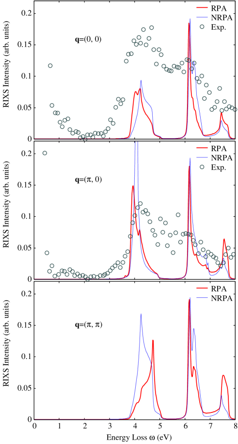
Figure 2: (Color online) Calculated results of RIXS spectra for three momentum transfers ${\mib q}=(0,0),(\pi,0),(\pi,\pi)$, and comparison with experimental results at ${\mib q}=(0,0),(\pi,0)$. The empty circles represent experimental data read from Ref. References. The thick red and thin blue lines represent the results calculated with and without RPA, respectively.

Comparing the peak positions between the cases with and without RPA, the 4 eV peak is shifted to the high energy region due to electron correlations at ${\mib q}=(\pi,\pi)$, while it is not at ${\mib q}=(0,0)$ and $(\pi,0)$.

Here, we present more detailed momentum dependence of the RIXS spectra than presented in the previous work by Takahashi et al. [52]. The detailed momentum dependence of RIXS spectra along the symmetry lines in the first BZ is shown by the intensity plot in Fig. 3.

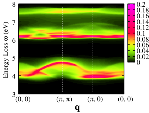
Figure 3: (Color online) Intensity plot of the RIXS spectra calculated for the undoped antiferromagnetic state. The horizontal axis represents the momentum transfer along the symmetry lines of the square BZ, and the vertical axis represents the energy loss of photons.

Our calculation suggests the possibility that the 4 eV peak exhibits stronger dispersion along the line $(0,0)$-$(\pi,\pi)$ rather than along the line $(0,0)$-$(\pi,0)$. This contrasts strongly with the case of La₂CuO₄, in which the 2 eV peak shows strong dispersion along $(0,0)$-$(\pi,0)$ [8].

To see the microscopic origin of the RIXS weights, we present the results of density of states (DOS) in Fig. 4. The insulating gap energy, which corresponds to the charge transfer energy between the Ni$3d$ and O$2p$ bands, is about 4 eV, being consistent with photoemission experiments [57]. The 4 eV RIXS spectral weight corresponds to the charge transfer excitations from the Ni$3d$-O$2p$ anti-bonding band to the Ni$3d$ upper Hubbard band.

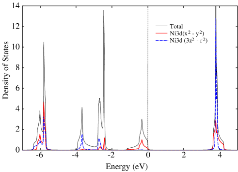
Figure 4: (Color online) Total and Ni$3d$ partial density of states are depicted. The total DOS, and the partial DOS for Ni$3d_{x^{2}-y^{2}}$ and Ni$3d_{3z^{2}-r^{2}}$ orbitals are represented by thin black, thick red solid and thick blue broken lines, respectively.

The 6 eV peak corresponds to the charge transfer excitation from the Ni-O bonding band to the upper Hubbard band.

3.2 Case of doped stripe-ordered states: $x=\frac{1}{3}$, ${\mib Q}_{s}=(\frac{2}{3}\pi,\frac{2}{3}\pi)$

As mentioned in the last paragraph of § 2.1, it may be impossible to determine all ${\mib u}_{ij}$’s by solving eq. (17) consistently with eq. (23). For example, let us focus on a Ni atom and its two neighboring O atoms whose two Ni-O bonds cross perpendicularly each other. If those two Ni-O bonds shrink (the O-Ni-O angle remains perpendicular), then the O-O bond length determined from eq. (23) necessarily shrinks. However, this shrinkage of the O-O bond is not necessarily consistent with ${\mib u}_{ij}$ determined for that O-O bond by using the condition eq. (17). For this difficulty, we may take the following way: firstly we determine ${\mib u}_{ij}$ for each nearest-neighbor Ni-O bond by using the condition eq. (17) (or equivalently eq. (21)), and then we determine ${\mib u}_{ij}$ for each nearest-neighbor O-O bond by using eq. (23). Fortunately, this treatment seems valid, as inferred from the following discussions. As far as we studied, if we determine all ${\mib u}_{ij}$’s (including those for O-O bonds) from eq. (17) (or equivalently eq. (21)) without using the condition eq. (23), then the electronic structure and ${\mib u}_{ij}$’s only negligibly depend on $K_{\rm O,O}$, while they depend strongly on $K_{\rm Ni,O}$. This means that the lattice distortions are strongly dominated by changes of Ni-O bond length and the contributions from O-O bonds are almost energetically negligible. Therefore, to determine ${\mib u}_{ij}$ for each nearest-neighbor O-O bond, we may neglect the condition eq. (17) for O-O bonds, and instead of that, we should use eq. (23). The condition eq. (23) for O-O bonds reduces in the momentum representation to

$${\mib u}_{{\mib Q}3,{\mib Q}^{\prime}4}\Bigl{(}\pm\frac{\hat{x}}{2}\pm\frac{\hat{y}}{2}\Bigr{)}=\sum_{{\mib Q}^{\prime\prime}}\Bigl{[}{\mib u}_{{\mib Q}+{\mib Q}^{\prime\prime}3,{\mib Q}^{\prime\prime}\ell}\Bigl{(}\pm\frac{\hat{x}}{2}\Bigr{)}e^{{\rm i}{\mib Q}^{\prime\prime}\cdot(\pm\frac{\hat{x}}{2})}\delta_{{\mib Q}^{\prime}}+{\mib u}_{{\mib Q}^{\prime\prime}\ell,{\mib Q}^{\prime}+{\mib Q}^{\prime\prime}4}\Bigl{(}\pm\frac{\hat{y}}{2}\Bigr{)}e^{{\rm i}{\mib Q}^{\prime\prime}\cdot(\pm\frac{\hat{y}}{2})}\delta_{\mib Q}\Bigr{]},$$ (36)

$${\mib u}_{{\mib Q}4,{\mib Q}^{\prime}3}\Bigl{(}\pm\frac{\hat{x}}{2}\pm\frac{\hat{y}}{2}\Bigr{)}=\sum_{{\mib Q}^{\prime\prime}}\Bigl{[}{\mib u}_{{\mib Q}+{\mib Q}^{\prime\prime}4,{\mib Q}^{\prime\prime}\ell}\Bigl{(}\pm\frac{\hat{y}}{2}\Bigr{)}e^{{\rm i}{\mib Q}^{\prime\prime}\cdot(\pm\frac{\hat{y}}{2})}\delta_{{\mib Q}^{\prime}}+{\mib u}_{{\mib Q}^{\prime\prime}\ell,{\mib Q}^{\prime}+{\mib Q}^{\prime\prime}3}\Bigl{(}\pm\frac{\hat{x}}{2}\Bigr{)}e^{{\rm i}{\mib Q}^{\prime\prime}\cdot(\pm\frac{\hat{x}}{2})}\delta_{\mib Q}\Bigr{]},$$ (37)

where $\ell$ is Ni $d$ orbital (i.e., $\ell=1$ or $2$), and the double signs in front of $\frac{\hat{x}}{2}$ (or $\frac{\hat{y}}{2}$) correspond in each equation.

We consider the following four self-consistent solutions (I)-(IV). (I): not allowing lattice distortions, we diagonalize $H_{\rm MF}$ from eq. (11) and use the self-consistency conditions eqs. (12) and (13). (II): allowing lattice distortions, we diagonalize $H_{\rm MF}+H_{\rm l.d.}$ from eqs. (11) and (19), and use the self-consistency conditions eqs. (12), (13) and (21), where we use eq. (21) only for Ni-O bonds and do not use eqs. (36) and (37) for O-O bonds. For (II), we take $K_{\rm Ni,O}=30$ eV. (III) and (IV): allowing lattice distortions, we use eq. (21) only for Ni-O bonds, and use eqs. (36) and (37) for nearest-neighbor O-O bonds. For (III) and (IV), we take $K_{\rm Ni,O}=30$ eV and $K_{\rm Ni,O}=60$ eV, respectively. These solutions are summarized in Fig. 5.

(a)

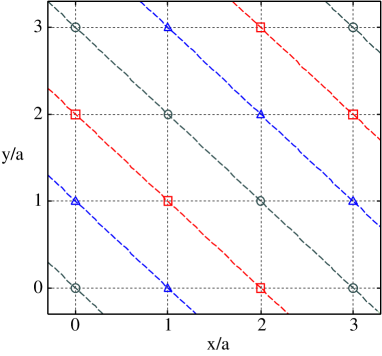
(b) HF stripe solution $n_{\bigcirc}$ $n_{\triangle}$ $n_{\square}$ $m_{\bigcirc}$ $m_{\triangle}$ $m_{\square}$ (I): no lattice distortions 2.16 2.20 2.16 1.59 -1.77 1.59 (II): $K_{\rm Ni,O}=30$ eV, 2.26 2.37 2.34         not using eqs. (36) and (37) 0.98 -1.45 1.40 (III): $K_{\rm Ni,O}=30$ eV, 2.30 2.39 2.35         using eqs. (36) and (37) 1.06 -1.42 1.31 (IV): $K_{\rm Ni,O}=60$ eV, 2.22 2.29 2.27         using eqs. (36) and (37) 1.24 -1.64 1.50

Figure 5: (Color online) (a) Schematic figure of diagonal stripe states with ${\mib Q}_{s}=(\frac{2}{3}\pi,\frac{2}{3}\pi)$. The same symbols represent equivalent Ni sites. (b) Typical stripe solutions within the HF calculation are presented. $n_{i}$’s and $m_{i}$’s ($i=\bigcirc,\triangle,\square$) are the electron occupation number and total spin moment (in units of $\mu_{\rm B}$), respectively, at Ni sites marked with the same symbols in (a).

Concerning lattice distortions in (II), nearest-neighbor Ni-O bonds shrink particularly around Ni sites with excess hole density ($\bigcirc$ sites in Fig. 5), being qualitatively consistent with previous studies [41, 47].

In Fig. 6, we present the calculated RIXS spectra in the low-energy region at various ${\mib q}$ points on the symmetry lines, for the stripe solution (III). A remarkable feature is that the low-energy edge of the spectra shows a tail toward the low-energy region at ${\mib q}={\mib Q}=(\frac{2}{3}\pi,\frac{2}{3}\pi)$.

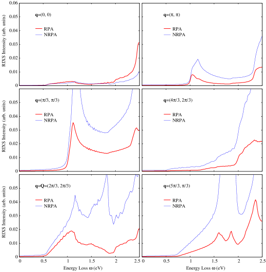
Figure 6: (Color online) Calculated RIXS spectra in the low-energy region at various momentum transfers for the stripe solution (III). In each panel, the thick red and thin blue lines represent the results calculated with and without RPA, respectively.

This is consistent with experimental results by Wakimoto et al. [37]. It should be noted that this low-energy tail appears already in the spectrum calculated without RPA, as shown in Fig. 6.

To see more detailed momentum dependence of the RIXS spectra on momentum transfer ${\mib q}$, we show intensity plots of the calculated RIXS spectra along the diagonal lines of the original square BZ for the stripe solutions (I)-(IV) in Fig. 7.

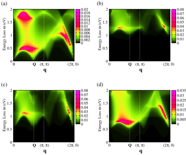
Figure 7: (Color online) Panels (a), (b), (c) and (d) show the intensity plots of calculated RIXS spectra for the four stripe solutions (I), (II), (III) and (IV), respectively

(see the text and Fig. 5 for the four stripe solutions). In each panel, the horizontal and vertical axes represent momentum transfer ${\mib q}$ and energy loss $\omega$, respectively, and ${\mib q}$ sweeps along the diagonals of the square BZ. ${\mib Q}=(\frac{2}{3}\pi,\frac{2}{3}\pi)$ is the stripe vector.

Comparing Fig. 7 with Fig. 3 of Ref. References, we consider that the RIXS intensity for the stripe state (III) is the most consistent with the experimental result. Comparing the spectra for the stripe states (II) and (III), we can see that shrinkage of nearest-neighbor O-O bonds, which is caused by shrinkage of nearest-neighbor Ni-O bonds, enhances the low-energy dispersive behavior around ${\mib q}\approx{\mib Q}$. Comparing the spectra for the stripe states (III) and (IV), we can see that the low-energy gap at ${\mib q}={\mib Q}$ becomes larger for smaller $K_{\rm Ni,O}$, i.e., for softer Ni-O bonds.

So far, we have considered only a single stripe-ordered domain characterized by the stripe vector ${\mib Q}_{s}=(\frac{2}{3}\pi,\frac{2}{3}\pi)$. To compare with the experimental results in more detail, we should bear in mind that, in addition to the above kind of domains, actual samples will contain also domains which correspond to ${\mib Q}_{s}=(\frac{4}{3}\pi,\frac{2}{3}\pi)$ (see Fig. 8(a)), as one can expect easily from tetragonal lattice symmetry. Here we assume that those two kinds of domains take evenly the same volume fraction in the sample, and the domain walls separating the domains only negligibly affect the RIXS spectra. Under this simple assumption, the total RIXS spectrum is given by the average of the contributions from the two kinds of domains. The averaged RIXS spectra for the stripe solution (III) are presented in Figs. 8(b) and (c) (compare Fig. 8(c) with Fig. 3 of Ref. References).

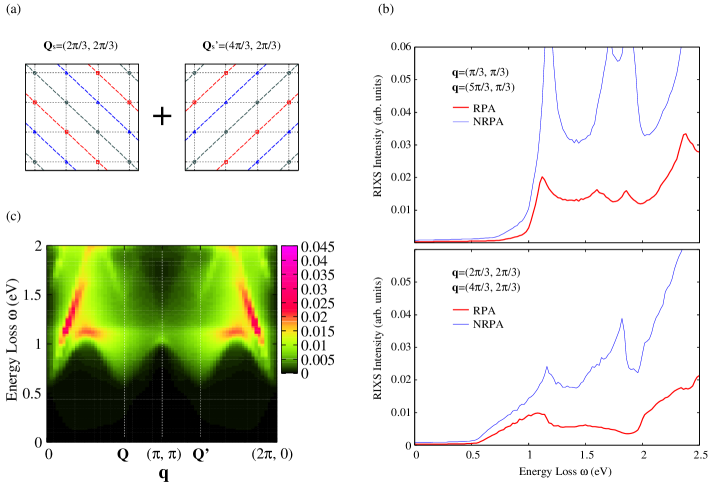
Figure 8: (Color online) (a) Schematic figure of two kinds of diagonal-stripe domains. (b) Averaged RIXS intensity from the two stripe domains at ${\mib q}=(\pi/3,\pi/3)$, $(2\pi/3,2\pi/3)$, $(4\pi/3,2\pi/3)$ and $(5\pi/3,\pi/3)$. The thick red and thin blue lines represent the results calculated with and without RPA, respectively. The spectra at ${\mib q}=(0,0)$ and $(\pi,\pi)$ are unchanged by taking the average, and are presented still by the upper two panels of Fig. 6. (c) Intensity plot of the averaged RIXS spectra. The horizontal and vertical axes represent momentum transfer ${\mib q}$ and energy loss $\omega$, respectively, and ${\mib q}$ sweeps along the diagonals of the square BZ.

According to the theoretical spectra (the upper two panels of Fig. 6 for ${\mib q}=(0,0)$ and $(\pi,\pi)$, and the two panels of Fig. 8(b) for ${\mib q}=(\pi/3,\pi/3)$, ${\mib q}=(2\pi/3,2\pi/3)$, ${\mib q}=(4\pi/3,2\pi/3)$ and $(5\pi/3,\pi/3)$), we see that the intensity at ${\mib q}=(0,0)$ and $(\pi,\pi)$ seems relatively weak compared with that at the other momentum transfers. One might consider that the weakness of the intensity at ${\mib q}=(0,0)$ is inconsistent with the strength of the experimental intensity at the point ‘A’ in Fig. 2 of Ref. References. However, we should note that, in general, the intensity around the $\Gamma$ point (i.e. ${\mib q}=(0,0)$) can be affected easily by several realistic factors which are not included in the present model. One of them is the effect of disorders in the sample. In doped systems, actual samples inevitably contain some disorders or disordered domain walls situated randomly, while doped carriers are assumed to form ideally periodic configuration in the theoretical model. In principle, such disordered fractions possessing no characteristic spatial periodicity contribute to the intensity at the $\Gamma$ point. Another possible factor is the long-range component of Coulomb interaction. In doped systems, the long-range Coulomb interaction can change the form of the RIXS spectra around the $\Gamma$ point [25]. In addition, the multiple scattering due to the core-hole potential may enhance the spectral intensity around ${\mib q}=(0,0)$, as mentioned in § 3.1. To take account of these effects thoroughly remains an interesting but still difficult future work.

To study the origin of the above-mentioned anomalous momentum dependence of RIXS spectra around ${\mib q}\approx{\mib Q}$, we present the electron energy dispersions for the stripe solutions in Fig. 9. In Fig. 9, only the majority (i.e., up) spin bands are depicted for the cases (I), (III) and (IV).

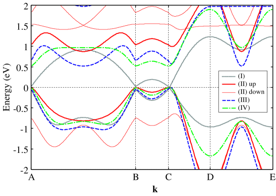
Figure 9: (Color online) Energy dispersions along the symmetry lines of the reduced BZ (Fig. 1) in the four stripe states (I)-(IV) (see the text and Fig. 5). For (I), (III) and (IV), only up (majority) spin bands are depicted, while both of the up and down spin bands are depicted for (II). Each symbol, A, $\cdots$, E, on the horizontal axis denotes the ${\mib k}$ point with the corresponding symbol in Fig. 1. The Fermi level is set to zero.

The calculated bands suggest the existence of gap minima around the symmetry points A, B and C (and the equivalent points), as seen in Fig. 9. As easily expected from this, the low-energy tail around ${\mib q}\approx{\mib Q}$ in RIXS spectra originates from the charge excitations between those symmetry points. Such gap minima may be observable by angle-resolved photoemission spectroscopy (ARPES).

4 Discussions and Conclusions

We have presented the RIXS spectra calculated for undoped insulating antiferromagnet La₂NiO₄ and stripe-ordered La_5/3Sr_1/3NiO₄, where we have described the ground state by the HF approximation and have taken account of electron correlations within RPA. For the undoped case, we have explained the spectral peak positions semiquantitatively, and have presented a more detailed plot than in the previous work. In the experiment by Collart et al. [15], the momentum-transfer dependence along the line $(0,0)$-$(\pi,0)$ was studied in detail. However, our present calculation suggests that the low-energy peak around 4 eV shows stronger dispersion along $(0,0)$-$(\pi,\pi)$ rather than along $(0,0)$-$(\pi,0)$. This contrasts with the case of the insulating cuprate La₂CuO₄. Experimental verification of this suggestion is awaited.

For doped stripe-ordered La_5/3Sr_1/3NiO₄, we have explained the anomalous momentum-transfer dependence of spectra observed experimentally, i.e., the calculated RIXS spectra show a tail toward the low-energy region when the momentum transfer of photons equals stripe vector ${\mib Q}=(\frac{2}{3}\pi,\frac{2}{3}\pi)$, being consistent with the recent experimental result by Wakimoto et al [37]. The reason for the low-energy tail at ${\mib Q}$ is that the gap minima of electron energy dispersion in the stripe-ordered states exist around the symmetry points A$(\frac{14}{9}\pi,\frac{4}{9}\pi)$, B$(\frac{4}{9}\pi,\frac{14}{9}\pi)$, C$(\frac{2}{9}\pi,\frac{10}{9}\pi)$ and the equivalent points in momentum space. This feature of the energy bands in stripe-ordered La_5/3Sr_1/3NiO₄ may be verified by ARPES experiments.

We searched for other possible self-consistent solutions than presented in Fig. 5 (b), by choosing various initial values of $n_{i\ell}$, $m_{i\ell}$ and ${\mib u}_{ij}$ in numerical iterations. However, we found only the equivalent solutions, which are obtained by rearranging ($n_{\bigcirc},m_{\bigcirc}$), ($n_{\triangle},m_{\triangle}$) and ($n_{\square},m_{\square}$) or by reversing the signs of spin moments. The stripe states with lattice distortions ((II), (III) and (IV) in Fig. 5 (b)) are not symmetric under spatial inversion. This does not mean that the electron energy and RIXS spectra are not symmetric under inversion in momentum space. In fact, the obtained electron energy dispersions are symmetric (see the dispersions along the D-E line in Fig. 9). We checked numerically that the RIXS spectra are also symmetric under inversion in wave vector space, as a result from the symmetry of the electron energy dispersion.

For the case of stripe ordered states, we have presented theoretical results of the RIXS spectra only for the relatively low-energy region (0-2.5eV, as in Figs. 6, 7 and 8). We should note that the RIXS spectra calculated for doped stripe states within the present formulation are reliable only in such low-energy region, while those for the undoped antiferromagnetic state are reliable up to the high-energy region. For the undoped case, the HF approximation presents large magnetic moments ($m_{i1}=0.78,m_{i2}=0.96$), and consequently the two magnetically split bands with an enough large energy gap mimic well the actual Hubbard bands, which are separated by the Mott-Hubbard gap of the order of $U$. In this case, the electronic structure in the actual antiferromagnetic ground state of the Mott insulating phase is well described over a wide energy range up to the order of $U$ by the HF approximation. On the other hand, in the doped stripe states, the magnetic moments are reduced ($m_{i1}=0.22$-0.54, $m_{i2}=0.85$-0.88, for the stripe solution (III)), compared with the undoped case. In this case, the electronic structure only inside the reduced magnetic gap can be still described by the HF approximation, although the high-energy Hubbard satellite bands are no longer reproduced. Very roughly speaking, the magnetic gap for orbital $\ell$ within the HF calculation is evaluated to be $\Delta_{i\ell}\sim Um_{i\ell}+J\sum_{\ell^{\prime}(\neq\ell)}m_{i\ell^{\prime}}$. According to this rough evaluation, $\Delta_{i\ell}\sim 2.6$-7.5 eV for the stripe solution (III), while $\Delta_{i\ell}\sim 7.2$-8.5 eV for the undoped antiferromagnetic ground state. Thus, for the doped stripe-ordered cases, the calculated RIXS spectra are reliable only in the low-energy region up to about 2.6 eV. To study RIXS spectra in such doped Mott insulators over a wider energy range, we require more advanced methods such as the dynamical mean-field theory (DMFT) [58].

As we have discussed, the bond shrinkage between nearest-neighbor O-O sites seems important to obtain that low-energy anomalous dispersion quantitatively consistent with the experimental data. This is related to the fact that the doped holes occupy mainly the O2$p$ orbitals. The RIXS spectra reflect the momentum distribution of the partial component of the Ni3$d$ states mixed with the O2$p$ states. Therefore, change of the O-O bonding length (or, in other words, change of the O2$p$ band width) affects strongly the low-energy RIXS spectra, although the contribution of O-O bonding is energetically negligible as mentioned in § 3.2.

In conclusion, we would like to point out that the anomalous low-energy RIXS weight at the stripe vector ${\mib Q}$ does not indicate some kinds of collective charge excitation modes, since it can be explained at least qualitatively within simple band-to-band transitions. This physical picture seems consistent with the robustness of the charge ordering observed under high electric fields [59, 60].

- [1] A. Kotani and S. Shin: Rev. Mod. Phys. 73 (2001) 203.
- [2] A. Kotani: Eur. Phys. J. B 47 (2005) 3.
- [3] L.J.P. Ament, M. van Veenendaal, T.P. Devereaux, J.P. Hill and J. van den Brink: Rev. Mod. Phys. 83 (2011) 705.
- [4] J.P. Hill, C.C. Kao, W.A.L. Caliebe, M. Matsubara, A. Kotani, J.L. Peng and R.L. Greene: Phys. Rev. Lett. 80 (1998) 4967.
- [5] P. Abbamonte, C.A. Burns, E.D. Isaacs, P.M. Platzman, L.L. Miller, S.W. Cheong and M.V. Klein: Phys. Rev. Lett. 83 (1999) 860.
- [6] M.Z. Hasan, E.D. Isaacs, Z.X. Shen, L.L. Miller, K. Tsutsui, T. Tohyama and S. Maekawa: Science 288 (2000) 1811.
- [7] M.Z. Hasan, P.A. Montano, E.D. Isaacs, Z.X. Shen, H. Eisaki, S.K. Shinha, Z. Islam, N. Motoyama and S. Uchida: Phys. Rev. Lett. 88 (2002) 177403.
- [8] Y.J. Kim, J.P. Hill, C.A. Burns, S. Wakimoto, R.J. Birgeneau, D. Casa, T. Gog and C.T. Venkataraman: Phys. Rev. Lett. 89 (2002) 177003.
- [9] Y.J. Kim, J.P. Hill, H. Benthien, F.H.L. Essler, E. Jeckelmann, H.S. Choi, T.W. Noh, N. Motoyama, K.M. Kojima, S. Uchida, D. Casa and T. Gog: Phys. Rev. Lett. 92 (2004) 137402.
- [10] K. Ishii, K. Tsutsui, Y. Endoh, T. Tohyama, K. Kuzushita, T. Inami, K. Ohwada, S. Maekawa, T. Masui, S. Tajima, Y, Murakami and J. Mizuki: Phys. Rev. Lett. 94 (2005) 187002.
- [11] K. Ishii, K. Tsutsui, Y. Endoh, T. Tohyama, S. Maekawa, M. Hoesch, K. Kuzushita, M. Tsubota, T. Inami, J. Mizuki, Y. Murakami and K. Yamada: Phys. Rev. Lett. 94 (2005) 207003.
- [12] L. Lu, G. Chabot-Couture, X. Zhao, J.N. Hancock N. Kaneko, O.P. Vajk, G. Yu, S. Grenier, Y.J. Kim, D. Casa, T. Gog, M. Greven: Phys. Rev. Lett. 95 (2005) 217003.
- [13] S. Suga, S. Imada, A. Higashiya, A. Shigemoto, S. Kasai, M. Sing, H. Fujiwara, A. Sekiyama, A. Yamasaki, C. Kim, T. Nomura, J. Igarashi, M. Yabashi and T. Ishikawa: Phys. Rev. B 72 (2005) 081101.
- [14] A. Shukla, M. Calandra, M. Taguchi, A. Kotani, G. Vanko and S.W. Cheong: Phys. Rev. Lett. 96 (2006) 077006.
- [15] E. Collart, A. Shukla, J.P. Rueff, P. Leininger, H. Ishii, I. Jarrige, Y.Q. Cai, S.W. Cheong and G.D. Dhalenne: Phys. Rev. Lett. 96 (2006) 157004.
- [16] D.S. Ellis, J.P. Hill, S. Wakimoto, R.J. Birgeneau, D. Casa, T. Gog and Y.J. Kim: Phys. Rev. B 77 (2008) 060501.
- [17] T. Inami, T. Fukuda, J. Mizuki, S. Ishihara, H. Kondo, H. Nakao, T. Matsumura, K. Hirota, Y. Murakami, S. Maekawa and Y. Endoh: Phys. Rev. B 67 (2003) 045108.
- [18] S. Grenier, J.P. Hill, V. Kiryukhin, W. Ku, Y.J. Kim, K.J. Thomas, S.W. Cheong, Y. Tokura, Y. Tomioka, D. Casa and T. Gog: Phys. Rev. Lett. 94 (2005) 047203.
- [19] C.C. Kao, W.A.L. Caliebe, J.B. Hastings and J.M. Gillet: Phys. Rev. B 54 (1996) 16361.
- [20] M. Takahashi, J. Igarashi and T. Nomura: Phys. Rev. B 75 (2007) 235113.
- [21] T. Nomura and J. Igarashi: Phys. Rev. B 71 (2005) 035110.
- [22] J. Igarashi, M. Takahashi and T. Nomura: Phys. Rev. B 74 (2006) 245122.
- [23] J. van den Brink and M. van Veenendaal: Europhys. Lett. 73 (2006) 121.
- [24] R.S. Markiewicz and A. Bansil: Phys. Rev. Lett. 96 (2006) 107005.
- [25] R.S. Markiewicz, M.Z. Hasan and A. Bansil: Phys. Rev. B 77 (2008) 094518.
- [26] Y.J. Kim, J.P. Hill, S. Wakimoto, R.J. Birgeneau, F.C. Chou, N. Motoyama, K.M. Kojima, S. Uchida, D. Casa and T. Gog: Phys. Rev. B 76 (2007) 155116.
- [27] J.P. Hill, G. Blumeberg, Y.J. Kim, D.S. Ellis, S. Wakimoto, R.J. Birgeneau and S. Komiya, Y. Ando, B. Liang, R.L. Greene, D. Casa, T. Gog: Phys. Rev. Lett. 100 (2008) 097001.
- [28] D.S. Ellis, J. Kim,. J.P. Hill, S. Wakimoto, R.J. Birgeneau, Y. Shvyd’ko, D. Casa, T. Gog K. Ishii, K. Ikeuchi, A. Paramekanti and Y.J. Kim: Phys. Rev. B 81 (2010) 085124.
- [29] V. Sachan, D.J. Buttrey, J.M. Tranquada, J.E. Lorenzo and G. Shirane: Phys. Rev. B 51 (1995) 12742.
- [30] J.M. Tranquada, D.J. Buttrey and V. Sachan: Phys. Rev. B 54 (1996) 12318.
- [31] S.H. Lee and S.W. Cheong: Phys. Rev. Lett. 79 (1997) 2514.
- [32] H. Yoshizawa, T. Kakeshita, R. Kajimoto, T. Tanabe, T. Katsufuji and Y. Tokura: Phys. Rev. B 61 (2000) R854.
- [33] J.M. Tranquada, D.J. Buttrey, V. Sachan and J.E. Lorenzo: Phys. Rev. Lett. 73 (1994) 1003.
- [34] J.M. Tranquada, J.E. Lorenzo, D.J. Buttrey and V. Sachan: Phys. Rev. B 52 (1995) 3581.
- [35] J.M. Tranquada, B.J. Sternlieb, J.D. Axe, Y. Nakamura and S. Uchida: Nature 375 (1995) 561.
- [36] S.A. Kivelson, I.P. Bindloss, E. Fradkin, V. Oganesyan, J.M. Tranquada, A. Kapitulnik and C. Howald: Rev. Mod. Phys. 75 (2003) 1201.
- [37] S. Wakimoto, H. Kimura, K. Ishii, K. Ikeuchi, T. Adachi, M. Fujita, K. Kakurai, Y. Koike, J. Mizuki, Y. Noda, K. Yamada, A.H. Said and Y. Shvyd’ko: Phys. Rev. Lett. 102 (2009) 157001.
- [38] D. Poilblanc and T.M. Rice: Phys. Rev. B 39 (1989) 9749.
- [39] H.J. Schulz: Phys. Rev. Lett. 64 (1990) 1445.
- [40] M. Kato, K. Machida, H. Nakanishi and M. Fujita: J. Phys. Soc. Jpn. 59 (1990) 1047.
- [41] J. Zaanen and P.B. Littlewood: Phys. Rev. B 50 (1994) 7222.
- [42] J. Zaanen and A.M. Oles: Ann. Physik 508 (1996) 224.
- [43] T. Mizokawa and A. Fujimori: Phys. Rev. B 56 (1997) 11920.
- [44] M. Ichioka and K. Machida: J. Phys. Soc. Jpn. 68 (1999) 4020.
- [45] E. Kaneshita, M. Ichioka and K. Machida: J. Phys. Soc. Jpn. 70 (2001) 866.
- [46] M. Raczkowski, R. Frésard and A.M. Oleś: Phys. Rev. B 73 (2006) 094429.
- [47] E. Kaneshita and A.R. Bishop: J. Phys. Soc. Jpn. 77 (2008) 123709.
- [48] W.A. Harrison: Electronic Structure and the Properties of Solids (Dover Publications, Inc., New York, 1989).
- [49] T. Nomura and J. Igarashi: J. Phys. Soc. Jpn. 73 (2004) 1677.
- [50] M. Takahashi, J. Igarashi and T. Nomura: J. Phys. Soc. Jpn. 77 (2008) 034711.
- [51] T. Semba, M. Takahashi and J. Igarashi: Phys. Rev. B 78 (2008) 155111.
- [52] M. Takahashi, J. Igarashi and T. Semba: J. Phys: Condens. Matter 21 (2009) 064236.
- [53] P. Nozières and E. Abrahams: Phys. Rev. B 10 (1974) 3099.
- [54] K. Tsutsui, T. Tohyama and S. Maekawa: Phys. Rev. Lett. 83 (1999) 3705.
- [55] K. Tsutsui, T. Tohyama and S. Maekawa: Phys. Rev. Lett. 91 (2003) 117001.
- [56] K. Okada and A. Kotani: J. Phys. Soc. Jpn. 75 (2006) 044702.
- [57] H. Eisaki, S. Uchida, T. Mizokawa, H. Namatame, A. Fujimori, J. van Elp, P. Kuiper, G.A. Sawatzky, S. Hosoya and H. Katayama-Yoshida: Phys. Rev. B 45 (1992) 12513.
- [58] A. Georges, G. Kotliar, W. Krauth and M.J. Rozenberg: Rev. Mod. Phys. 68 (1996) 13.
- [59] S. Yamanouchi, Y. Taguchi and Y. Tokura: Phys. Rev. Lett. 83 (1999) 5555.
- [60] M. Hücker, M. v. Zimmerman and G.D. Gu: Phys. Rev. B 75 (2007) 041103.