Hamilton’s turns as visual tool-kit for designing of single-qubit unitary gates

Abstract

Unitary evolutions of a qubit are traditionally represented geometrically as rotations of the Bloch sphere, but the composition of such evolutions is handled algebraically through matrix multiplication [of SU(2) or SO(3) matrices]. Hamilton’s construct, called turns, provides for handling the latter pictorially through the as addition of directed great circle arcs on the unit sphere S${}^{2}\subset\mathbb{R}^{3}$, resulting in a non-Abelian version of the parallelogram law of vector addition of the Euclidean translation group. This construct is developed into a visual tool-kit for handling the design of single-qubit unitary gates. As an application, it is shown, in the concrete case wherein the qubit is realized as polarization states of light, that all unitary gates can be realized conveniently through a universal gadget consisting of just two quarter-wave plates (QWP) and one half-wave plate (HWP). The analysis and results easily transcribe to other realizations of the qubit: The case of NMR is obtained by simply substituting $\pi/2$ and $\pi$ pulses respectively for QWPs and HWPs, the phases of the pulses playing the role of the orientation of fast axes of these plates.

I Introduction

States of a qubit are in one-to-one correspondence with points of the (solid) unit ball $D^{3}\subset\mathbb{R}^{3}\,$($D$ for disk); depending on the context it is called the Poincaré or Bloch ball. Pure states are on the boundary S² of $D^{3}$ and mixed states correspond to the interior points. The von Neumann entropy which is a measure of the mixedness of the state $\rho$ has the simple form

$$S(\rho)=-\sum_{\pm}\,\frac{1\pm r}{2}{\rm log}_{2}\frac{1\pm r}{2},\;\;0\leq r\leq 1,$$

where $r$ is the radial distance of the point representing the state measured from the center of $D^{3}$. When the qubit is realized as polarization states of light, $r$ equals the degree of polarization oneil ; wolf . The center corresponds to the maximally mixed (completely unpolarized) state.

To go with this attractive geometric portraying of states, unitary evolutions $\rho\to U\rho\,U^{\dagger},~{}U\in$ SU(2) act as (three-dimensional) rotations leaving the center of the state space $D^{3}$ invariant. This is a realization of the adjoint representation of SU(2) as the two-to-one SU(2) $\to$ SO(3) homomorphism, both $U$ and $-\,U$ of SU(2) imaging to the same element of SO(3). More general physical evolutions or channels act as inhomogeneous linear maps on $D^{3}$; in addition to mapping $D^{3}$ into itself, some additional requirement amounting to complete positivity davis-book will have to be satisfied by these maps. Such nonunitary evolutions, however, play no role in this work.

Though states and their (unitary) evolutions are thus represented geometrically, composition or concatenation of evolutions is traditionally handled algebraically through matrix multiplication. Hamilton’s turns hamilton-lectures offer a visual tool for handling this last aspect too in a geometrical or vivid pictorial manner. In this picture, unitary evolutions are represented by (equivalence classes of) directed great circle arcs on S², with composition of unitary evolutions correctly represented by a geometric addition rule for these directed arcs, quite analogous to the manner in which translation group elements in an Euclidean space are composed using the parallelogram law of vector addition.

An extensive description of Hamilton’s construct may be found in the book of Biedenharn and Louck biedenharn-book , while a simplified presentation of the addition rule for turns is given more recently in Ref. turns-sc . An early application of this construct to polarization optics can be found in turns-pramana , and generalization of the construct to other low-dimensional groups can be be found in turns-prl ; turns-jmp ; turns-juarez ; turns-vssc .

The principal aim of the present work is to develop Hamilton’s geometric construct into a tool-kit for handling the composition and synthesis of unitary single-qubit gates in an efficient pictorial manner with no recourse to matrix multiplication. To be concrete, it is assumed in much of the presentation that our qubit is realized as polarization states of a photon photon-qubit1 ; photon-qubit2 ; kimble , but transliteration to other realizations of the qubit will be evident. For instance, the case of NMR quantum computation is easily seen to correspond to quarter-wave plates (QWPs) and half-wave plates (HWPs) being replaced, respectively, by $\pi/2$ and $\pi$ pulses, the phases of the pulses playing the role of the orientation of the fast axis of the plates.

The tool-kit presented has the obvious limitation that it can handle only single-qubit (unitary) gates. Even so it could prove to be of value to quantum computation in view of the fact that single-qubit gates, along with just one two-qubit gate like the C-NOT gate, can realize all multi-qubit gates nielsen ; gates-deutsch ; gates-barenco ; gates-divincenzo .

The usefulness of this tool-kit is not limited to the domain of quantum information and computation. The group SU(2) pervades many areas of science, either directly or through the rotation group ${\rm SO(3)}={\rm SU(2)}/Z_{2}$, and this tool-kit could therefore prove useful in these other areas as well. In particular, it is of direct interest to classical polarization optics.

The entire presentation shoots towards the main result formulated as a theorem at the end of the paper, which asserts that all single-qubit gates can be conveniently realized using a universal gadget consisting of just two QWPs and one HWP. We should hasten to add, however, that this theorem is not new in itself, but has been formulated earlier using algebraic methods gadget-minimal , and Bagini et al. gadget-gori have presented a particularly helpful exposition of this result of Ref. gadget-minimal which has been variously used used1 ; used2 ; used3 ; used4 ; used5 ; used6 ; used7 . Whereas the algebraic approach took a sequence of several papers turns-pramana ; gadget-bhandari ; gadget-universal to eventually arrive at the final result in the fourth gadget-minimal , through a sequesnce of false starts and refinements, the pictorial approach presented here will be seen to render the result visual, and almost obvious.

Since this geometric construct of Hamilton, called turns does not appear to be as well known as it deserves to be, we begin with a description of this construct itself, relating it to the three prominent parametrizations of SU(2)—the homogeneous Euler, the axis-angle, and the Euler parametrizations—and bringing out its interesting connection with the Berry-Pancharatnam geometric phase.

II HAMILTON’S TURNS

Reversible gates acting on a qubit are in one-to-one correspondence with $2\times 2$ unitary matrices $u\in$ SU(2). The SU(2) matrices can be conveniently described by any triplet $\tau_{1},\tau_{2},\tau_{3}$ of Pauli-like Hermitian matrices satisfying the defining algebraic relations

$$\tau_{k}\tau_{l}=\delta_{kl}\tau_{0}+i\epsilon_{klm}\tau_{m},$$ (1)

where $\tau_{0}=\mathbbm{1}_{2\times 2}$ is the unit matrix $\in$ SU(2). To be specific, we take these matrices to be $\tau_{1}=\sigma_{3},\tau_{2}=\sigma_{1}$ and $\tau_{3}=\sigma_{2}$, where $\sigma_{j}$’s are the standard Pauli matrices. The family of all unitary (reversible single-qubit) gates $u\in$ SU(2) then get parametrized as

$$u = a_{0}\tau_{0}-i\bm{a}\cdot\bm{\tau}=\left(\begin{array}[]{clcr}a_{0}-ia_{1}&&-ia_{2}-a_{3}\\ \\ -ia_{2}+a_{3}&&a_{0}+ia_{1}\par\end{array}\right),$$ (6)

$$a_{0}^{2}+a_{1}^{2}+a_{2}^{2}+a_{3}^{2}\equiv a_{0}^{2}+\bm{a}\cdot\bm{a}=1.$$

That is, the four real parameters $(a_{0},\bm{a})=(a_{0},a_{1},a_{2},a_{3})$, called the homogeneous Euler parameters, correspond to a point on the three-sphere S${}^{3}\subset\mathbb{R}^{4}$. Elements of SU(2) are thus in one-to-one correspondence with points on S³, consistent with and exhibiting the fact that S³ is the group manifold of SU(2). Hamilton’s turns constitute a powerful visual representation of this S${}^{3}\subset{\mathbb{R}}^{4}$ on S${}^{2}\subset{\mathbb{R}}^{3}$ through (equivalence classes of) directed great circle arcs, with group multiplication of SU(2) matrices (concatenation of single-qubit unitary gates) faithfully transcribed into a ”parallelogram law of addition” for these directed geodesic arcs on S².

Given a unitary gate $u$ or $(a_{0},\bm{a})\in$ S³, the constraint $a_{0}^{2}+\bm{a}\cdot\bm{a}=1$ guarantees that we can find an ordered pair of unit vectors $\bm{\hat{n}}_{1},\,\bm{\hat{n}}_{2}\in\mathbb{R}^{3}$ such that

$$a_{0}=\bm{\hat{n}}_{1}\cdot\bm{\hat{n}}_{2},~{}~{}~{}~{}~{}\bm{a}=\bm{\hat{n}}_{1}\wedge\bm{\hat{n}}_{2}.$$ (7)

It follows that a directed great circle (or geodesic) arc on S², with tail at $\bm{\hat{n}}_{1}$ and head at $\bm{\hat{n}}_{2}$, can be associated with the unitary gate $u$. Clearly, such an association is not unique, and the non-uniqueness is precisely to the following extent: Any pair $\bm{\hat{n}}_{1}^{\prime},\,\bm{\hat{n}}_{2}^{\prime}$ obtained by rotating both $\bm{\hat{n}}_{1}$ and $\bm{\hat{n}}_{2}$ by equal amount about $\bm{\hat{n}}_{1}\wedge\bm{\hat{n}}_{2}$ will meet the requirements in Eq. (7), and hence will correspond to the gate represented by the original pair $\bm{\hat{n}}_{1},\bm{\hat{n}}_{2}$. Such a rotation obviously corresponds to rigidly sliding the directed arc representing $u$ along its great circle.

One is thus led to consider equivalence classes of directed great circle arcs on S², the equivalence being with respect to the sliding just noted: Two such directed arcs are equivalent if they are on the same great circle and if one can be made to coincide with the other by rigidly sliding it on the great circle. These equivalence classes are called Hamilton’s turns. It is clear that elements of SU(2) are in one-to-one correspondence with turns (assuming the arclength of turns is restricted not to exceed $\pi$).

If $u\in$ SU(2) is represented by the turn whose representative element is the directed great circle arc from $\bm{\hat{n}}_{1}$(tail) to $\bm{\hat{n}}_{2}$(head), we denote this fact through

$$u=T(\bm{\hat{n}}_{1},\bm{\hat{n}}_{2})=\bm{\hat{n}}_{1}\cdot\bm{\hat{n}}_{2}-i\bm{\hat{n}}_{1}\wedge\bm{\hat{n}}_{2}\cdot\bm{\tau}.$$ (8)

Henceforth we talk of turns, SU(2) matrices, and unitary single-qubit gates interchangeably. For brevity, we often call a representative arc itself as the turn and its length as the length of the turn or simply as the turn length, but this abuse of terminology should cause no confusion.

Two special elements of SU(2) namely $\tau_{0}$ and $-\tau_{0}$ are distinguished in that they constitute the center of the group. This distinction should be expected to manifest itself in any representation, and the one due to Hamilton happens to be no exception. The unit element $\tau_{0}$, the trivial gate, corresponds to the null turn $\bm{\hat{n}}_{1}=\bm{\hat{n}}_{2}\in$ S², and the gate $\,-\tau_{0}$ to $\bm{\hat{n}}_{1}=-\bm{\hat{n}}_{2}\in S^{2}$, the respective turn-lengths being $0,\,\pi$. The equivalence class associated with either is clearly a two-parameter family, since $\bm{\hat{n}}_{1}$ can be any point on S². However, the equivalence class of directed great circle arcs associated with any other turn is a one-parameter family. In particular, every turn or $u\in\,$SU(2), $u\neq\pm\tau_{0}$, has associated with it a unique directed great circle of S².

Analogy with the Euclidean translation group (in two dimensions, for instance) wherein group elements are represented by equivalence classes of ‘free vectors’ is obvious. There the abelian group composition takes the geometric form of parallelogram law of vector addition. It turns out that such a geometric or pictorial composition of group elements applies to the present non-Abelian case of SU(2) as well, with turns playing the role of (equivalence classes of) free vectors; indeed, the power of Hamilton’s turns can be traced to this fascinating fact.

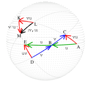
Figure 1: The ”parallelogram law” or ”addition rule” for turns, with ${\rm turn~{}AB\;=\;turn~{}BE}$ and ${\rm turn~{}BC\;=\;turn~{}DB}$ representing, respectively, unitary gates $u$ and $v$ and ${\rm turn~{}AC}$ and ${\rm turn~{}DE}$ representing, respectively, the products $vu$ and $uv$. Since ${\rm turn~{}LK}$ represents $vu$ and ${\rm turn~{}KM}$, the inverse of ${\rm turn~{}DE}$, represents $v^{-1}u^{-1}$, and ${\rm turn~{}LM}$ represents the commutator $[v,\,u]=v^{-1}u^{-1}vu$.

To see this pictorial composition law, assume that we are given two SU(2) gates $u,v$ and we wish to compute geometrically (visually) the matrix product $vu$. Referring to Fig. 1, let the directed great circle arc AB represent $u$ and let BC represent $v$. It is important to note that the representative arcs are so chosen that the head of the right factor $u$ and the tail of the left factor $v$ coincide at B$\,\sim\,\bm{\hat{n}}_{2}$; since great circles on S² certainly intersect, this can always be arranged for any given pair of turns. Now draw the directed geodesic arc from the free tail A$\,\sim\,\bm{\hat{n}}_{1}$ to the free head C$\,\sim\,\bm{\hat{n}}_{3}$ to obtain a new turn represented by the directed arc AC. The important claim is that turn AC correctly represents the matrix product $vu$. This is readily verified through matrix multiplication:

$$vu = T(\bm{\hat{n}}_{2},\bm{\hat{n}}_{3})T(\bm{\hat{n}}_{1},\bm{\hat{n}}_{2})$$ (9)

$$= (\bm{\hat{n}}_{2}\cdot\bm{\hat{n}}_{3}-i\bm{\hat{n}}_{2}\wedge\bm{\hat{n}}_{3}\cdot\bm{\tau})(\bm{\hat{n}}_{1}\cdot\bm{\hat{n}}_{2}-i\bm{\hat{n}}_{1}\wedge\bm{\hat{n}}_{2}\cdot\bm{\tau})$$

$$= \bm{\hat{n}}_{1}\cdot\bm{\hat{n}}_{3}-i\bm{\hat{n}}_{1}\wedge\bm{\hat{n}}_{3}\cdot\bm{\tau}=T(\bm{\hat{n}}_{1},\bm{\hat{n}}_{3}).$$

Remark: The only property of the $\tau$-matrices used in this verification is $\tau_{k}\tau_{l}=\delta_{kl}\tau_{0}+i\epsilon_{klm}\tau_{m}$, and hence this result and its consequences are independent of which set of Pauli-like matrices was actually used.

We forced ourselves to perform the kind of matrix multiplication in Eq. (9), just once, simply to demonstrate that the one-to-one correspondence between SU(2) gates and turns is indeed a group isomorphism. The rest of this work, however, will rest solely on the geometric or visual construct of turns, with almost no recourse to matrix multiplication. We note in passing that the above composition law immediately implies that the matrix inverse of the SU(2) gate or turn $T(\bm{\hat{n}}_{1},\bm{\hat{n}}_{2}$) corresponds to $T(\bm{\hat{n}}_{2},\bm{\hat{n}}_{1}$), the reversed turn.

To compute or construct the ‘other’ product $uv$, choose E and D on the great circles, respectively, through A, B and C, B such that AB = BE and BC = DB. Then turn BE = turn AB represents $u$ and turn DB = turn BC represents $v$. It is thus obvious in view of Eq. (9), that turn DE represents the product $uv$, which is manifestly different from the product $vu$ (represented by turn AC), giving a vivid pictorial depiction of the noncommutative nature of the ”addition rule” for turns, consistent with the non-Abelian nature of SU(2) composition.

Remark: In spite of being quite different from one another, turn AB and turn DE share one important common aspect. To see this, consider the spherical triangles ABC and EBD. The angle at B is the same for both triangles, AB = BE, and CB = BD. The two triangles are thus congruent, showing that turn AC and turn DE have the same turn length. As we shall see, this is a pictorial manifestation of the fact ${\rm tr}\,vu={\rm tr}\,uv$.

Presented also in Fig. 1 is a visual display of the commutator of two SU(2) gates. Recall that the commutator of a pair of elements $g_{1},\,g_{2}$ of a multiplicative group $G$ is defined as $[g_{2},\,g_{1}]\equiv g_{2}^{-1}g_{1}^{-1}g_{2}g_{1}$, the multiplicative difference of $g_{1}g_{2}$ and $g_{2}g_{1}$. Let the geodesic arcs DE and AC when extended meet at K. Choose points L, M on these extended arcs such that AC = LK and ED = KM. Since turn EB corresponds to $u^{-1}$ and turn BD to $v^{-1}$, turn ED corresponds to the product $v^{-1}u^{-1}=(uv)^{-1}$. Referring now to the spherical triangle LKM, since turn LK corresponds to $vu$ and turn KM to $v^{-1}u^{-1}$ we deduce, again in view of Eq. (9), that turn LM corresponds to the product $v^{-1}u^{-1}vu$, the commutator $[v,\,u]$ of interest.

It is often convenient to rewrite the SU(2) composition rule of matrix multiplication

$$T(\bm{\hat{n}}_{3},\bm{\hat{n}}_{4})T(\bm{\hat{n}}_{2},\bm{\hat{n}}_{3})T(\bm{\hat{n}}_{1},\bm{\hat{n}}_{2})=T(\bm{\hat{n}}_{1},\bm{\hat{n}}_{4})$$ (10)

as the geometric (visual) rule of ”addition” of turns

$$\mbox{turn}~{}\bm{\hat{n}}_{1}\bm{\hat{n}}_{2}+\mbox{turn}~{}\bm{\hat{n}}_{2}\bm{\hat{n}}_{3}+\mbox{turn}~{}\bm{\hat{n}}_{3}\bm{\hat{n}}_{4}=\mbox{turn}~{}\bm{\hat{n}}_{1}\bm{\hat{n}}_{4}.$$ (11)

In transcribing from the ”multiplication” mode of Eq. (10) to the ”addition” mode of Eq. (11), however, it is important to remember that the individual terms in this ”sum” in Eq. (11) read from left to right correspond to the factors in the SU(2) matrix product Eq. (10) read from right to left; the order is important, the ”sum” being non-commutative. This geometric ”addition rule” for turns, which is clearly reminiscent of the parallelogram law for the composition of elements of the (Abelian) Euclidean translation group, is associative and faithfully represents the non-Abelian or non-commutative group composition in SU(2).

Our consideration of turns so far has been based on the homogeneous Euler parametrization of SU(2) Eq. (2). The group SU(2) can also be parametrized in the axis-angle form

$$u=u(\bm{\hat{n}},\alpha) \equiv \exp(-i\frac{\alpha}{2}\bm{\hat{n}}\cdot\bm{\tau})$$

$$= \cos\frac{\alpha}{2}\,\tau_{0}-i\sin\frac{\alpha}{2}\,\bm{\hat{n}}\cdot\bm{\tau};$$

$$u(\bm{\hat{n}},2\pi) = -\tau_{0},\;\;\;u(\bm{\hat{n}},4\pi)=\tau_{0},\;\;$$

$$u(\bm{\hat{n}},2\pi+\alpha) = u(-\bm{\hat{n}},2\pi-\alpha),$$ (12)

where $\bm{\hat{n}}$ is a unit vector $\in{\mathbb{R}}^{3}$. We may, in view of the last line of Eq. (II), restrict $\alpha$ to the range $0\leq\alpha\leq 2\pi$. A view of turns which corresponds to this parametrization proves more convenient for some purposes, and so we describe it briefly.

We have seen that every turn, other than the special turns $T(\bm{\hat{n}},\bm{\hat{n}})$ and $T(\bm{\hat{n}},-\bm{\hat{n}})$ corresponding to elements in the center of SU(2), has associated with it a unique directed great circle; this great circle and an angle (length of the representative arc) fully specifies the turn. However, directed great circles and directed axes (or unit vectors $\bm{\hat{n}}\in S^{2}$) are in one-to-one correspondence: if the directed great circle is specified by the ordered pair $(\bm{\hat{n}}_{1},\bm{\hat{n}}_{2})$ of linearly independent unit vectors, the directed axis is specified by the unit vector $\bm{\hat{n}}\in S^{2}$ in the direction of $\bm{\hat{n}}_{1}\wedge\bm{\hat{n}}_{2}$. We may thus denote a turn alternatively by the symbol $T(\bm{\hat{n}},\alpha)$, with the understanding that the representative directed arc is on the great circle orthogonal to $\bm{\hat{n}}$ and has arclength $\alpha$. In other words, $T(\bm{\hat{n}},\alpha)$ corresponds to $u(\bm{\hat{n}},2\alpha)\in\,$ SU(2). With the two special turns excluded, it is clear that this representation is unique [ $\bm{\hat{n}}_{1}\wedge\bm{\hat{n}}_{2}$ is nonvanishing for every $u$ not in the center of SU(2), that is, for every turn whose turn-length$~{}\in(0,\pi)\,$].

We note from the last line of Eq. (II) that $T(\bm{\hat{n}},\pi+\alpha)=T(-\bm{\hat{n}},\pi-\alpha)$, and hence the restriction of $\alpha$, the turn-length, to the range $0\leq\alpha\leq\pi$. For the two special turns corresponding to the center of SU(2), we see that $T(\bm{\hat{n}},0)$ and $T(\bm{\hat{n}},\pi)$ represent, respectively, $\tau_{0}$ and $-\tau_{0}$, independent of $\bm{\hat{n}}\in S^{2}$.

We note in passing a direct relationship between the turn length and the trace of the associated SU(2) matrix. Indeed, the facts that ${\rm tr}\,u(\bm{\hat{n}},\alpha)=2\cos\frac{\alpha}{2}$ and $u(\bm{\hat{n}},2\alpha)\in\,$SU(2) is represented by the turn $T(\bm{\hat{n}},\alpha)$ of length $\ell_{u}=\alpha$ show that ${\rm tr}\,u=2\cos\ell_{u}$. In particular, ${\rm tr}\,u$ is positive or negative depending on whether the turn length $\ell_{u}$ is $<$ or $>\pi/2$ : All traceless SU(2) matrices correspond to turn-length $\pi/2$, the popular Hadamard gate nielsen and HWPs considered below being examples.

III Realization of qubit as polarization states of light

As indicated earlier, our illustrations demonstrating the power of turns in solving problems of synthesis of unitary gates will use the concrete context wherein qubit is realized as the polarization states of light. However, it is evident from the treatment to follow that the entire analysis applies equally well to other realizations of qubits and SU(2) gates, like NMR quantum computation nielsen or passive (lossless) linear optics of a pair of radiation modes at lossless beam splitters saleh .

Birefringent media play a particularly dominant role in polarization optics, both classical and quantum. Consider a (quasi-monochromatic) light beam propagating along the positive $x_{3}$ direction of a Cartesian system $(x_{1},x_{2},x_{3})$. The components $E_{1},E_{2}$ of the transverse electric field along the $x_{1},x_{2}$ directions can be arranged into a column vector $E\in{\mathcal{C}}^{2}$, called the Jones vector of the polarization state of the beam oneil . The intensity equals $|E_{1}|^{2}+|E_{2}|^{2}=E^{\dagger}E$. A linear optical system is correspondingly represented by a $2\times 2$ numerical matrix $J$ called the Jones matrix, and the input-output relationship is represented by

$$E_{\rm in}\rightarrow E_{\rm out}=JE_{\rm in}.$$ (13)

Lossless linear systems conserve intensity: $E^{\dagger}_{\rm out}E_{\rm out}=E^{\dagger}_{\rm in}E_{\rm in}$. It follows that the Jones matrices of such systems are unitary. Birefringent media, which introduce a relative phase between a characteristic pair of orthogonal linear polarization states, and optically active media which introduce a relative phase between the two (orthogonal) circular polarization states are examples of such lossless linear systems of interest to polarization optics. Suppressing an overall phase, the Jones matrices of lossless linear systems can be identified with elements of the unimodular unitary group SU(2). In the case wherein the qubit corresponds to the polarization states of a photon, these are indeed the relevant unitary or reversible single qubit gates.

A birefringent plate (compensator) whose ”fast axis” is along the transverse $x_{1}$ direction has the Jones matrix

$$J=C_{0}(\eta) = \left(\begin{array}[]{clcr}e^{-i\eta/2}&0\\ 0&e^{i\eta/2}\end{array}\right)$$ (16)

$$= \exp\left(-i\frac{\eta}{2}\tau_{1}\right)\in{\rm SU(2)},$$ (17)

$\eta$ being the relative phase introduced by the plate; we have $\eta=\epsilon\,\ell/\lambda$, where $\ell$ is the thickness of the plate, $\epsilon>0$ is the difference between the refractive indices for the two characteristic orthogonal linear polarizations, and $\lambda$ is the wavelength. It is clear that if the fast axis is at an angle $\varphi$ with the $x_{1}$ axis, then the Jones matrix would be

$$J = C_{\varphi}(\eta)=\Phi(\varphi)C_{0}(\eta)\Phi(\varphi)^{-1}$$

$$= \cos(\eta/2)\,\tau_{0}\,-i\,\sin(\eta/2)\,(\cos(2\varphi)\,\tau_{1}+\sin(2\varphi)\,\tau_{2}),$$

where the two-dimensional matrix

$$\Phi(\varphi)=\exp(-i\varphi\tau_{3})=\left(\begin{array}[]{clcr}\cos\varphi&&-\sin\varphi\\ \sin\varphi&&\cos\varphi\end{array}\right)$$ (19)

is an element of the subgroup SO(2) $\subset$ SU(2).

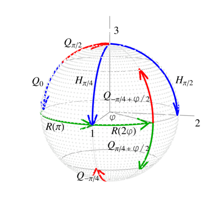
Figure 2: The sphere of turns ${\cal T}$ as it applies to the polarization qubit. All turns on the equator (horizontal turns) correspond to optical rotators, and vertical turns correspond to birefringent plates. While relating to the subscripts of HWPs and QWPs it should be remembered that spatial rotation of magnitude $\varphi/2$ is reflected on ${\cal T}$ as polar rotation of magnitude $\varphi$ and not $\varphi/2$.

Quarter-wave plates (QWPs) and half-wave plates (HWPs) are particular cases of birefringent plates and correspond, respectively, to $\eta=\pi/2$ and $\pi$; they could equally well be called $\lambda/4$ and $\lambda/2$ plates. The Jones matrix of a QWP with fast axis along the $x_{1}$-direction is thus $\exp(-i\frac{\pi}{4}\tau_{1})=(\tau_{0}-i\tau_{1})/\sqrt{2}$; we denote this QWP by $Q_{0}$, so that $Q_{\varphi}=\Phi(\varphi)Q_{0}\Phi(\varphi)^{-1}=[\,\tau_{0}-i(\tau_{1}\cos 2\varphi+\tau_{2}\sin 2\varphi)\,]/\sqrt{2}$ represents the QWP whose fast axis makes an angle $\varphi$ with the positive $x_{1}$ axis. Similarly, we use the notation $H_{0}$ for the HWP $-i\tau_{1}$ so that $H_{\varphi}$ stands for $\Phi(\varphi)H_{0}\Phi(\varphi)^{-1}=-i(\tau_{1}\cos 2\varphi+\tau_{2}\sin 2\varphi)$, a HWP whose fast axis makes angle $\varphi$ with the $x_{1}$ axis. In particular, $H_{\varphi/8}$ corresponds to the Hadamard gate nielsen . Thus $H_{\varphi}=(\,Q_{\varphi}\,)^{2}$, for all $\varphi$. These are particular cases of a more general and evident fact: If an optical system represented by Jones matrix $J$ is physically rotated by an angle $\varphi$ about the positive $x_{3}$ axis, the resulting system will have Jones matrix $\exp(-i\varphi\tau_{3})J\exp(i\varphi\tau_{3})$.

The SO(2) matrix $\exp(-i\varphi\tau_{3})$ plays yet another role in polarization optics: It is also the Jones matrix of an optically active medium. Specifically, an optically active medium (or simply optical rotator) which introduces a relative phase $\alpha$ between the left and the right circularly polarized states has the Jones matrix

$$R(\alpha)=\exp(-i\frac{\alpha}{2}\tau_{3}).$$ (20)

Numerically, $R(\alpha)=\Phi(\alpha/2)$; however, we have chosen to use a different symbol $R(\alpha)$ for the optical rotator to distinguish it from $\Phi(\cdot)$, which stands for physical rotation of a gadget in the transverse plane.

We depict in Fig. 2 the sphere of turns ${\cal T}$. It is clear that all ”vertical turns” correspond to birefringent plates: QWPs and HWPs have turn lengths of $\pi/4$ and $\pi/2$, respectively. Turns on the equator correspond to optical rotators.

In addition to the homogeneous Euler and axis-angle parametrizations of SU(2) gates already considered there exists a third one, the Euler angle parametrization,

$$u = u(\xi,\eta,\zeta)$$ (21)

$$\equiv \exp(-i\frac{1}{2}\xi\tau_{3})\,\exp(-i\frac{1}{2}\eta\tau_{1})\,\exp(-i\frac{1}{2}\zeta\tau_{3}).~{}~{}~{}~{}$$

This parametrization of the SU(2) group of unitary gates can be viewed as saying that every such gate is equivalent to an appropriate birefringent plate $C_{0}(\eta)$ sandwiched between two appropriate optically active media $R(\xi),\,R(\zeta)$, with the effective thicknesses of the three media engineered to match the Euler parameters $\xi,\eta,\zeta$ of the gate under consideration. However, from an experimenter’s point of view this cannot be the most convenient realization of the various unitary gates $J\in$  SU(2); unlike the HWP and QWP, $C_{0}(\eta)$ is not a component readily available off the shelf, and a variable $R(\xi)$ tends to introduce $\xi$-dependent loss and dynamical phase. It turns out that QWPs and HWPs alone are sufficient. As we will see, the geometric representation of Hamilton renders this fact particularly transparent and visual.

We may note in passing that the Euler angle parametrization [Eq. (21)] can be rewritten in the modified form

$$u(\xi,\eta,\zeta)=C_{\xi/2}(\eta)\,R({\xi+\zeta})=R({\xi+\zeta})\,C_{-\zeta/2}(\eta).~{}~{}~{}$$ (22)

This means an arbitrary unitary gate is a variable birefringent plate preceded or followed by a variable rotator. The fact still remains that, unlike QWPs and HWPs, variable birefringent plates are nonstandard polarization optical components, and optically active media introduce undesirable losses and dynamical phases which vary with the optical rotation or effective thickness of the medium.

IV Hamilton’s turns and transformation of polarization states

Polarization states are conveniently described (even in the classical case) by restricting attention to Jones vectors of unit norm (unit intensity) and ignoring an overall phase. Such normalized Jones vectors correspond, in the quantum case, to state vectors of a two-level system or qubit. In either case, the state represented by a normalized Jones vector E is fully determined by the (complex) ratio $z=E_{2}/E_{1}$. This is rendered particularly transparent by going over to the coherency or density matrix, and one then finds that polarization states are in one-to-one correspondence with points on the unit sphere S², called the Poincaré or Riemann sphere, obtained by identifying the points $z\to\infty$ (the one-point compactification) of the complex $z$ plane:

$$\mbox{tr}(EE^{\dagger}) = 1~{}~{}\mbox{and}~{}~{}e^{i\alpha}E(\bm{\hat{m}})\sim E(\bm{\hat{m}}),~{}~{}~{}\bm{\hat{m}}\in S^{2},$$

$$\rightarrow \rho(\bm{\hat{m}})\equiv E(\bm{\hat{m}})E(\bm{\hat{m}})^{\dagger}.\;\,$$

Written in more detail,

$$E(\bm{\hat{m}})=\frac{1}{\sqrt{2}}\left(\begin{array}[]{cr}e^{-i\varphi/2}\cos\frac{\theta}{2}+e^{i\varphi/2}\sin\frac{\theta}{2}\\ \\ \;i\left(e^{-i\varphi/2}\cos\frac{\theta}{2}-e^{i\varphi/2}\sin\frac{\theta}{2}\right)\\ \end{array}\right),~{}~{}~{}$$ (26)

so that for any state $\bm{\hat{m}}\in{\rm S}^{2}$ we have for the ratio $z(\bm{\hat{m}})$ of the components of $E(\bm{\hat{m}})$ the expression

$$z(\bm{\hat{m}})=\frac{E_{2}}{E_{1}}=\frac{\sin\theta\sin\varphi+i\cos\theta}{1+\sin{\theta}\cos{\varphi}}.$$ (27)

The corresponding coherency or density matrix reads

$$\rho(\bm{\hat{m}}) = E(\bm{\hat{m}})E(\bm{\hat{m}})^{\dagger}$$

$$= \frac{1}{2}\left(\begin{array}[]{clcr}1+\sin\theta\cos\varphi&&\;\sin\theta\sin\varphi-i\cos\theta\\ \\ \sin\theta\sin\varphi+i\cos\theta&&1-\sin\theta\cos\varphi\\ \end{array}\right)$$

$$= \frac{1}{2}(\tau_{0}+\bm{\hat{m}}\cdot\bm{\hat{\tau}});$$

$$z(\bm{\hat{m}}) = \rho_{12}(\bm{\hat{m}})/\rho_{11}(\bm{\hat{m}}).$$ (32)

The parameters $\theta,\varphi$ are respectively the polar and azimuthal coordinates of $\bm{\hat{m}}=(\sin\theta\cos\varphi,\,\sin\theta\sin\varphi,\,\cos\theta)\in S^{2}$.

Had we used in place of the ”$\tau$ matrices” the standard Pauli $\sigma$ matrices, the coherency matrix would have read

$$\rho(\bm{\hat{m}})=\frac{1}{2}(\sigma_{0}+\bm{\hat{m}}\cdot\bm{\sigma})=\frac{1}{2}\left(\begin{array}[]{clcr}1+\cos\theta&&\;e^{-i\varphi}\sin\theta\\ \\ e^{i\varphi}\sin\theta&&1-\cos\theta\\ \end{array}\right).$$ (36)

[$\sigma_{0}$ again is the unit matrix $\mathbbm{1}_{2\times 2}=\tau_{0}$.] Consequently, $E(\bm{\hat{m}})$ would have been parametrized as

$$E(\bm{\hat{m}})=\left(\begin{array}[]{clcr}\cos\theta/2\\ \\ e^{i\varphi}\sin\theta/2\end{array}\right),$$ (41)

so that the ratio $E_{2}/E_{1}$ becomes $z(\bm{\hat{m}})=e^{i\varphi}\,\tan(\theta/2)$, a form more familiar in the context of NMR and the associated Bloch sphere.

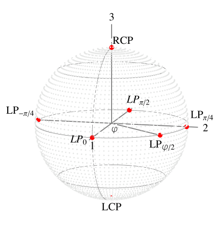
Figure 3: The polarization states of light represented as points on the Poincaré sphere ${\cal P}$. Right and left circularly polarized states occupy the polar positions, and points on the equator correspond to linear polarization states. Spatial rotation of the plane of polarization by angle $\varphi$ corresponds to $2\varphi$ rotation about the polar axis. Thus linear polarization ${\rm LP}_{0}$ along the $x_{1}$ axis and linear polarization ${\rm LP}_{\pi/4}$ at $45^{\circ}$ to the $x_{1}$ axis are separated on ${\cal P}$ by $90^{\circ}$. Points of the upper (lower) hemisphere correspond, respectively, to right (left) handed elliptic polarization.

Staying with the choice $\tau$, rather than $\sigma$, we sketch in Fig. 3 the Poincaré sphere $\mathcal{P}$. We adopt the convention that right and left circular polarization (RCP and LCP) states correspond, respectively, to $\frac{1}{\sqrt{2}}\left(\begin{array}[]{clcr}1\\ i\end{array}\right)$ and $\frac{1}{\sqrt{2}}\left(\begin{array}[]{clcr}1\\ -i\end{array}\right)$ or, equivalently, to the Poincaré sphere coordinates $(0,0,1)$ for RCP and $(0,0,-1)$ for LCP. Linear polarization at angle $\alpha$ to the (positive) $x_{1}$ axis has Jones vector $\left(\begin{array}[]{clcr}\cos\alpha\\ \sin\alpha\end{array}\right)$ and corresponds to the Poincaré sphere coordinates $(\cos 2\alpha,\sin 2\alpha,0)$. Thus, all linear polarization states are on the equator; all states above the equator have right-handed elliptic polarization, while those in the lower hemisphere are left-handed. Antipodal points of $\mathcal{P}$ correspond to orthogonal polarization states: $E(-\bm{\hat{m}})^{\dagger}E(\bm{\hat{m}})=0$, equivalently ${\rm tr}\,(\,\rho(-\bm{\hat{m}})\rho(\bm{\hat{m}})\,)=0$.

Remark on convention: Since the expressions for $E(\bm{\hat{m}})$ and $\rho(\bm{\hat{m}})$ may ”appear to be” considerably simpler with the choice $\bm{\sigma}$, one may wonder why one chose $\bm{\tau}$ in the first place. The reason is one of convention, a price one occasionally pays for tradition. In the case of a spin-$\frac{1}{2}$ particle of the NMR context or a two-level atom, one chooses the vectors $\left(\begin{array}[]{clcr}1\\ 0\end{array}\right)$ and $\left(\begin{array}[]{clcr}0\\ 1\end{array}\right)$ to correspond to the poles of S² and prefers to associate Bloch’s name with this sphere. Obviously, these so-called computational basis states are eigenstates of $\sigma_{3}$. In polarization optics, on the other hand, the circularly polarized states $\frac{1}{\sqrt{2}}\left(\begin{array}[]{clcr}1\\ \pm i\end{array}\right)$ are given the special honor of polar positions, but these are eigenstates of $\sigma_{2}=\tau_{3}$. Following tradition we wish to keep the polar axis as the vertical and third axis for polarization qubit. Cyclic permutation of the $\sigma$ matrices seems to be the minimal way of meeting these concerns or requirements without offending in any way the basic algebra [ commutation and anti-commutation relations, Eq. (1) ].

V Action of turns on the Poincaré sphere and connection with geometric phase

The notation $T(\bm{\hat{n}},\alpha)$ for turns, corresponding to the axis-angle parametrization $u(\bm{\hat{n}},\,2\alpha)=\exp(-i{\alpha}\,\bm{\hat{n}}\cdot\bm{\tau})$ of SU(2), proves convenient in exhibiting the action of turns on the Poincaré sphere, our state space. Unitary gates $T(\bm{\hat{n}},\alpha)$ act on the Poincaré sphere, that is, on state $\rho(\bm{\hat{m}})=\frac{1}{2}[\tau_{0}+\bm{\hat{m}}\cdot\bm{\tau}]$ represented by $\bm{\hat{m}}\in{\cal P}$, in this manner:

$$T(\bm{\hat{n}},\alpha):\;\;\rho(\bm{\hat{m}}) \to \rho(\bm{\hat{m}}^{\,\prime})=T(\bm{\hat{n}},\alpha)\,\rho(\bm{\hat{m}})\,T(\bm{\hat{n}},\alpha)^{\,-1}$$

$$= \exp(-i\,{\alpha}\,\bm{\hat{n}}\cdot\bm{\tau})\,\rho(\bm{\hat{m}})\,\exp(i\,\alpha\,\bm{\hat{n}}\cdot\bm{\tau}).$$

As expected, the two special gates $\tau_{0},\,-\tau_{0}$ corresponding to elements of the center of SU(2) are seen to have no effect on the Poincaré sphere and, as noted earlier, the set of parameters $(\bm{\hat{n}},\alpha)$ in $T(\bm{\hat{n}},\alpha)$, with $0<\alpha<\pi$, is unique for every other turn.

Now, in view of the algebraic properties of the $\tau$ matrices [Eq. (1)], the above transformation law simply reduces to

$$T(\bm{\hat{n}},\alpha):\;\;\bm{\hat{m}}\to\bm{\hat{m}}^{\,\prime}=(\bm{\hat{m}}\cdot\bm{\hat{n}})\bm{\hat{n}} + \cos 2\alpha[\bm{\hat{m}}-(\bm{\hat{m}}\cdot\bm{\hat{n}})\bm{\hat{n}}]$$ (43)

$$+ \sin 2\alpha\,\bm{\hat{n}}\wedge\bm{\hat{m}}.$$

Note that $(\bm{\hat{m}}\cdot\bm{\hat{n}})\bm{\hat{n}}$ is the component of $\bm{\hat{m}}$ along $\bm{\hat{n}}$ and $\bm{\hat{m}}-(\bm{\hat{m}}\cdot\bm{\hat{n}})\bm{\hat{n}}$ is the component of $\bm{\hat{m}}$ orthogonal to $\bm{\hat{n}}$ and hence in the plane spanned by $\bm{\hat{m}},\bm{\hat{n}}$. Further $\bm{\hat{n}}\wedge\bm{\hat{m}}$ which is orthogonal to both $\bm{\hat{m}}$ and $\bm{\hat{n}}$ has the same magnitude as $\bm{\hat{m}}-(\bm{\hat{m}}\cdot\bm{\hat{n}})\bm{\hat{n}}$. Thus, the effect of $T(\bm{\hat{n}},\alpha)$ on the state space or Poincaré sphere ${\cal P}$ is an SO(3) rotation about $\bm{\hat{n}}$, of extent $2\alpha=$ twice the length of the turn. In particular, the three one-parameter subgroups of SU(2) gates $\exp(\,-i\,\frac{\alpha_{k}}{2}\,\tau_{k}\,),\;\,k=1,2,3~{}$, act on ${\cal P}$, respectively, through the following one-parameter subgroups of SO(3) rotations:

$$\exp(\,-i\,\frac{\alpha_{1}}{2}\,\tau_{1}\,)\to{\cal R}_{1}(\alpha_{1})=\left(\begin{array}[]{ccc}1&0&0\\ ~{}0{}&\cos\alpha_{1}&-\sin\alpha_{1}\\ 0&\sin\alpha_{1}&\cos\alpha_{1}\end{array}\right)\,,$$ (47)

$$\exp(\,-i\,\frac{\alpha_{2}}{2}\,\tau_{2}\,)\to{\cal R}_{2}(\alpha_{2})=\left(\begin{array}[]{ccc}\cos\alpha_{2}&~{}0{}&\sin\alpha_{2}\\ 0&1&0\\ -\sin\alpha_{2}&0&\cos\alpha_{2}\end{array}\right)\,,$$ (51)

$$\exp(\,-i\,\frac{\alpha_{3}}{2}\,\tau_{3}\,)\to{\cal R}_{3}(\alpha_{3})=\left(\begin{array}[]{ccc}\cos\alpha_{3}&-\sin\alpha_{3}&~{}0{}\\ \sin\alpha_{3}&\cos\alpha_{3}&0\\ 0&0&1\end{array}\right)\,.$$ (55)

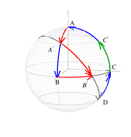
Figure 4: Shown on the sphere of turns ${\cal T}$ is a geodesic triangle corresponding to a unitary resolution of identity. While ${\rm turns~{}AB,\;\;BC,\;\,CA}$ compose to unity, their respective square roots compose to ${\rm turn~{}B^{\prime}C}$ whose turn length is half the area of the triangle.

Now consider the spherical triangle ABC on the sphere of turns ${\cal T}$ shown in Fig. 4, the coordinates of A,B,C being respectively $(0,0,1),\,(1,0,0),\,(0,1,0)$. Since turn AB corresponds to the unitary gate $-i\tau_{2}$, turn BC to $-i\tau_{3}$, and turn CA to $-i\tau_{1}$, the (closed) triangular circuit,

$${\rm turn~{}AB}+{\rm turn~{}BC}+{\rm turn~{}CA}={\rm null~{}turn}$$ (57)

represents a visual depiction of the matrix product identity

$$(-i\tau_{1})\,(-i\tau_{3})\,(-i\tau_{2})=\tau_{0}$$ (58)

involving the Pauli gates—, a unitary resolution of the identity.

Let A^′, B^′, and C^′ be the midpoints of AB, BC, and CA respectively. Thus, ${\rm turn~{}AA^{\prime}}={\rm turn~{}A^{\prime}B}$, ${\rm turn~{}BB^{\prime}}={\rm turn~{}B^{\prime}C}$ and ${\rm turn~{}CC^{\prime}}={\rm turn~{}C^{\prime}A}$ are the square roots of ${\rm turn~{}AB}$, ${\rm turn~{}BC}$, and ${\rm turn~{}CA}$, respectively. It is instructive to compute the composition of these square-root turns: ${\rm turn~{}AA^{\prime}}+{\rm turn~{}BB^{\prime}}+{\rm turn~{}CC^{\prime}}$. Note that ${\rm AA^{\prime}}$, ${\rm BB^{\prime}}$, and ${\rm CC^{\prime}}$ have equal arclength of $\pi/4$, and correspond respectively to $\frac{1}{\sqrt{2}}(\tau_{0}-i\tau_{2})$, $\frac{1}{\sqrt{2}}(\tau_{0}-i\tau_{3})$, and $\frac{1}{\sqrt{2}}(\tau_{0}-i\tau_{1})$. Since ${\rm turn~{}AA^{\prime}}={\rm turn~{}A^{\prime}B}$, we have ${\rm turn~{}AA^{\prime}}+{\rm turn~{}BB^{\prime}}={\rm turn~{}A^{\prime}B^{\prime}}$. To compose ${\rm turn~{}A^{\prime}B^{\prime}}$ with ${\rm turn~{}CC^{\prime}}$ extend ${\rm A^{\prime}B^{\prime}}$ to meet the great circle through A and C at D. Comparing the spherical triangles ${\rm BB^{\prime}A^{\prime}}$ and ${\rm CB^{\prime}D}$, we see that ${\rm BB^{\prime}}={\rm B^{\prime}C}$, ${\rm angle~{}A^{\prime}BB^{\prime}}={\rm angle~{}B^{\prime}CD}$ $(=\pi/2)$, and ${\rm angle~{}BB^{\prime}A^{\prime}}={\rm angle~{}CB^{\prime}D}$. The two triangles are thus congruent, and so ${\rm turn~{}A^{\prime}B^{\prime}}={\rm turn~{}B^{\prime}D}$ and arclength of ${\rm DC}$ = arclength of ${\rm A^{\prime}B}$ $(=\pi/4)$. Thus, ${\rm turn~{}A^{\prime}B^{\prime}}+{\rm turn~{}CC^{\prime}}={\rm turn~{}B^{\prime}D}+{\rm turn~{}DC}={\rm turn~{}B^{\prime}C}={\rm turn~{}BB^{\prime}}$. We have thus shown

$${\rm turn~{}AA^{\prime}}+{\rm turn~{}BB^{\prime}}+{\rm turn~{}CC^{\prime}} = {\rm turn~{}BB^{\prime}},$$

$${\rm i.\,e.\,,}\;\,\sqrt{-i\tau_{1}}\,\sqrt{-i\tau_{3}}\,\sqrt{-i\tau_{2}}=\sqrt{-i\tau_{3}} = \frac{1}{\sqrt{2}}(\tau_{0}-i\tau_{3}).\;\;$$

The square roots thus compose to produce neither the null turn nor its square root (any turn of turn length =$\pi$), but $\frac{1}{\sqrt{2}}(\tau_{0}-i\tau_{3})$, a primitive eighth root of the null or identity turn $\tau_{0}$.

This is due to the following fact: Unlike triangles in the Euclidean plane, there is no notion of similar triangles (beyond congruence) in the spherical case; the area of a spherical triangle is fully determined by its three angles. This situation described by Eqs. (58) and (V) should be contrasted with the corresponding situation in respect of the Euclidean parallelogram law, wherein if three elements of the translation group compose to produce the null (identity), element then their respective ”square roots” too will certainly compose to yield the null element, corresponding to a similar triangle with one-fourth area and the same interior angles as the original one. The failure of the SU(2) turns in this respect, as depicted by Eq. (V), is rooted in the non-Abelian nature of the group on the one hand and in the nontrivial curvature of S² (as compared to the Euclidean plane) on the other; indeed, these two aspects go hand in hand, as may be seen also by consideration of the geometric or Pancharatnam phase.

Before we turn to the geometric phase, we note, however, that the sum of the three (interior) angles of the triangle ABC is in excess of $\pi$ by $\pi/2$, and this spherical excess equals the area of the triangle. We note also that the turn length of the composite ${\rm turn~{}AA^{\prime}}+{\rm turn~{}BB^{\prime}}+{\rm turn~{}CC^{\prime}}$, which is clearly a measure of the extent to which the square roots fail to compose to the null turn, is $\pi/4$, precisely half of the area of the original (closed) triangle ABC. That is, in the axis-angle notation $T({\bm{\hat{n}}},\alpha)$, the value of $\alpha$ corresponding to composition of the square roots (that is, ${\rm turn~{}B^{\prime}C}$) is $\pi/4$; and $\bm{\hat{n}}$ corresponds precisely to $\bm{\hat{n}}_{A}$, the ”starting point” A of the triangle.

All these aspects apply not only to the particular triangle shown in Fig. 4 but also to an arbitrary geodesic triangle; construction of proof in the general case is slightly more elaborate, but very similar to the one for the special triangle in Fig. 4 (see Ref. two-level ). That is, we have for any spherical triangle ABC with area ${\cal A}$

$${\rm turn~{}AA^{\prime}} + {\rm turn~{}BB^{\prime}}+{\rm turn~{}CC^{\prime}}=T(\bm{\hat{n}}_{A},\,{\cal A}/2),\;\;\;\;$$ (60)

where ${\rm A^{\prime},\;B^{\prime},\;C^{\prime}}$ are, respectively, the midpoints of AB, BC, CA and $\bm{\hat{n}}_{A}$ is the unit vector pointing in the direction of A $\in S^{2}$.

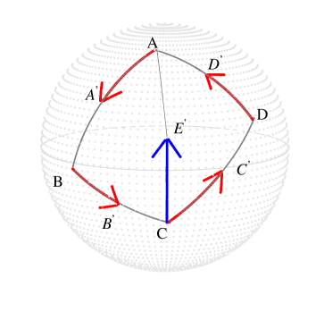
Figure 5: Generalization of the area formula of Fig. 4 to the case of a geodesic quadrilateral.

A simple argument implies that this area formula applies indeed to all geodesic polygons. Consider, for instance, the (geodesic) quadrilateral ABCD on ${\cal T}$ shown in Fig. 5. Let ${\rm A^{\prime}}$, ${\rm B^{\prime}}$, ${\rm C^{\prime}}$, ${\rm D^{\prime}}$ be the mid points of AB, BC, CD, and DA, respectively, and let ${\rm E^{\prime}}$ be the midpoint of the geodesic CA. Let ${\cal A}_{1}$ be the area of the triangle ABC and ${\cal A}_{2}$ that of ACD so that ${\cal A}={\cal A}_{1}+{\cal A}_{2}$ is the area of the quadrilateral, and let $\bm{\hat{n}}_{A}$ be the unit vector corresponding to the point A$\,\in{\cal P}$. We have the closed-circuit relation ${\rm turn~{}AB}+{\rm turn~{}BC}+{\rm turn~{}CD}+{\rm turn~{}DA}={\rm null~{}turn}$. We wish to compose the square roots of these turns in that order. The basic idea is to break this quadrilateral into two triangles ABC, ACD (making use of the fact that ${\rm turn~{}CE^{\prime}}+{\rm turn~{}AE^{\prime}}\,=\,{\rm null~{}turn}$). We have

$${\rm turn~{}AA^{\prime}} + {\rm turn~{}BB^{\prime}}+{\rm turn~{}CC^{\prime}}+{\rm turn~{}DD^{\prime}}$$ (61)

$$= ({\rm turn~{}AA^{\prime}}+{\rm turn~{}BB^{\prime}}+{\rm turn~{}CE^{\prime}})$$

$$~{}~{}+({\rm turn~{}AE^{\prime}}+{\rm turn~{}CC^{\prime}}+{\rm turn~{}DD^{\prime}})$$

$$= T(\bm{\hat{n}}_{A},\,{\cal A}_{1}/2)+T(\bm{\hat{n}}_{A},\,{\cal A}_{2}/2)$$

$$= T(\bm{\hat{n}}_{A},\,{\cal A}/2).$$

In the last step we used the fact that all turns $T(\bm{\hat{n}},\,\alpha)$ having the same $\bm{\hat{n}}$ form an (Abelian) one-parameter subgroup:

$$T(\bm{\hat{n}},\,\alpha)T(\bm{\hat{n}},\,\alpha^{\,\prime})=T(\bm{\hat{n}},\,\alpha^{\,\prime})T(\bm{\hat{n}},\,\alpha)=T(\bm{\hat{n}},\,\alpha+\alpha^{\,\prime}).$$

Generalization to $n$-sided geodesic polygons is obvious.

Remark: As a subtle but important aspect we may note that the addition rule in Eq. (V) and its covariance under SU(2) conjugation (which rigidly translocates the quadrilateral on the sphere S²) imply in turn the area formula in Eq. (61), namely that the second argument of $T$ should necessarily be proportional to the area of the triangle ABC.

Now we turn to the connection between geometric phase for two-level systems and the considerations of turns presented above. While geometric phase became popular owing to the seminal work of Berry berry1 , it had been ”anticipated” by Pancharatnam pancha , as pointed out by Nityananda and Ramaseshan nitya and subsequently by Berry berry2 . Some of the other works which could be viewed, in retrospect, to have anticipated the geometric phase are listed in Ref.  berry1 .

In the course of his interference experiments with polarized light Pancharatnam faced this question: Given two distinct (nonorthogonal) polarization states represented by linearly independent Jones vectors $E(\bm{\hat{n}}_{1})$ and $E(\bm{\hat{n}}_{2})$, when should one say that these Jones vectors are in phase? Motivated by his experiments, Pancharatnam arrived at the following answer: $E(\bm{\hat{n}}_{1})$ and $E(\bm{\hat{n}}_{2})$ are in phase if and only if the inner product $E(\bm{\hat{n}}_{1})^{\dagger}E(\bm{\hat{n}}_{2})$ is real positive. In other words, being in phase is synonymous with maximal constructive interference. He noted that ”being in phase” defined in this manner is not an equivalence relation, for it fails the transitivity requirement: $E(\bm{\hat{n}}_{1})$ being in phase with $E(\bm{\hat{n}}_{2})$ and $E(\bm{\hat{n}}_{2})$ being in phase with $E(\bm{\hat{n}}_{3})$ does not necessarily imply that $E(\bm{\hat{n}}_{3})$ is in phase with $E(\bm{\hat{n}}_{1})$. Indeed, he showed that this failure in respect of transitivity is geometric in nature, in the sense that if $E(\bm{\hat{n}}_{1})$ is in phase with $E(\bm{\hat{n}}_{2})$ and $E(\bm{\hat{n}}_{2})$ is in phase with $E(\bm{\hat{n}}_{3})$, then $E(\bm{\hat{n}}_{3})$ will be necessarily out of phase with $E(\bm{\hat{n}}_{1})$ precisely by half the area of the spherical triangle defined by vertices $\bm{\hat{n}}_{1},\,\bm{\hat{n}}_{2},\,\bm{\hat{n}}_{3}\in{\cal P}$.

As a simple illustration of this failure of transitivity, consider on the Poincaré sphere three points P, Q, R identified by unit vectors $\bm{\hat{n}}_{P}=(0,\,1,\,0)$, $\bm{\hat{n}}_{Q}=(0,\,0,\,1)$, and $\bm{\hat{n}}_{R}=(1,\,0,\,0)$ corresponding, respectively, to linear polarization at an angle $\pi/4$ to the $x_{1}$ axis, RCP, and linear polarization along the $x_{1}$ axis. The corresponding three Jones vectors may be taken to be

$$E(\bm{\hat{n}}_{P})=\frac{1}{\sqrt{2}}\left(\begin{array}[]{clcr}1\\ 1\end{array}\right), E(\bm{\hat{n}}_{Q})=\frac{1}{\sqrt{2}}e^{-i\,\pi/4}\left(\begin{array}[]{clcr}1\\ i\end{array}\right),$$ (67)

$$E(\bm{\hat{n}}_{R}) = e^{-i\,\pi/4}\left(\begin{array}[]{clcr}1\\ 0\end{array}\right).$$ (70)

We have chosen the phase factors multiplying $E(\bm{\hat{n}}_{Q})$, $E(\bm{\hat{n}}_{R})$ so as to ensure that $E(\bm{\hat{n}}_{P})$ is in phase with $E(\bm{\hat{n}}_{Q})$ and $E(\bm{\hat{n}}_{Q})$ in phase with $E(\bm{\hat{n}}_{R})$. It is readily verified that $E(\bm{\hat{n}}_{R})$ is indeed out of phase with $E(\bm{\hat{n}}_{P})$ by $\pi/4$, half the area of the spherical triangle PQR.

Given any three points $\bm{\hat{n}}_{1}$, $\bm{\hat{n}}_{2}$, $\bm{\hat{n}}_{3}$ on the Poincaré sphere, we may write out this failure of transitivity in the transparent form

$${\rm arg}\,[\,E(\bm{\hat{n}}_{1})^{\dagger}E(\bm{\hat{n}}_{2})\,E(\bm{\hat{n}}_{2})^{\dagger}E(\bm{\hat{n}}_{3})\,E(\bm{\hat{n}}_{3})^{\dagger}E(\bm{\hat{n}}_{1})\,]$$

$$={\rm arg}\,[\,{\rm tr}\,(\,E(\bm{\hat{n}}_{1})E(\bm{\hat{n}}_{1})^{\dagger}\,E(\bm{\hat{n}}_{2})E(\bm{\hat{n}}_{2})^{\dagger}\,E(\bm{\hat{n}}_{3})E(\bm{\hat{n}}_{3})^{\dagger}\,)\,]\;\,$$

$$={\rm arg}\,[\,{\rm tr}\,(\,\rho(\bm{\hat{n}}_{1})\,\rho(\bm{\hat{n}}_{2})\,\rho(\bm{\hat{n}}_{3}\,)\,]$$

$$~{}~{}\equiv\frac{1}{2}\,\Delta_{3}(\bm{\hat{n}}_{1},\,\bm{\hat{n}}_{2},\,\bm{\hat{n}}_{3}).$$ (71)

That $\Delta_{3}(\bm{\hat{n}}_{1},\,\bm{\hat{n}}_{2},\,\bm{\hat{n}}_{3})$ defined as above equals the area of the spherical triangle with vertices at $\bm{\hat{n}}_{1},\,\bm{\hat{n}}_{2},\,\bm{\hat{n}}_{3}\in{\cal P}$ is a result due to Pancharatnam. It may be noted that, $\Delta_{3}(\bm{\hat{n}}_{1},\,\bm{\hat{n}}_{2},\,\bm{\hat{n}}_{3})$, the argument of the product of pairwise inner products of ”successive” states, is manifestly gauge invariant in the sense that if the Jones vectors $E(\bm{\hat{n}}_{j})$ are replaced with $e^{i\alpha_{j}}E(\bm{\hat{n}}_{j})$, where $\alpha_{j},\;j=1,2,3$ are arbitrary phases, $\Delta_{3}(\bm{\hat{n}}_{1},\,\bm{\hat{n}}_{2},\,\bm{\hat{n}}_{3})$ remains unaffected [ every vector enters the expression as a bra and as a ket, once each ]. It is in view of this gauge invariance that $\Delta_{3}$ may be called a geometric phase.

If we are given four states corresponding to points $\bm{\hat{n}}_{1},\,\bm{\hat{n}}_{2},\,\bm{\hat{n}}_{3},\,\bm{\hat{n}}_{4}\in{\cal P}$, the associated gauge-invariant geometric object is

$${\rm arg}\,[E(\bm{\hat{n}}_{1})^{\dagger}E(\bm{\hat{n}}_{2})E(\bm{\hat{n}}_{2})^{\dagger}E(\bm{\hat{n}}_{3})E(\bm{\hat{n}}_{3})^{\dagger}E(\bm{\hat{n}}_{4})E(\bm{\hat{n}}_{4})^{\dagger}E(\bm{\hat{n}}_{1})]\;\,$$

$$~{}~{}~{}~{}={\rm arg}[E(\bm{\hat{n}}_{1})^{\dagger}E(\bm{\hat{n}}_{2})E(\bm{\hat{n}}_{2})^{\dagger}E(\bm{\hat{n}}_{3})E(\bm{\hat{n}}_{3})^{\dagger}E(\bm{\hat{n}}_{1})]$$

$$~{}~{}~{}~{}~{}~{}~{}+\,{\rm arg}[E(\bm{\hat{n}}_{1})^{\dagger}E(\bm{\hat{n}}_{3})E(\bm{\hat{n}}_{3})^{\dagger}E(\bm{\hat{n}}_{4})E(\bm{\hat{n}}_{4})^{\dagger}E(\bm{\hat{n}}_{1})]$$

$$~{}~{}~{}~{}\equiv\frac{1}{2}\Delta_{4}(\bm{\hat{n}}_{1},\,\bm{\hat{n}}_{2},\,\bm{\hat{n}}_{3},\,\bm{\hat{n}}_{4}),$$ (72)

where in the first step we simply inserted into the expression $E(\bm{\hat{n}}_{3})^{\dagger}E(\bm{\hat{n}}_{1})\,E(\bm{\hat{n}}_{1})^{\dagger}E(\bm{\hat{n}}_{3})=|\,E(\bm{\hat{n}}_{3})^{\dagger}E(\bm{\hat{n}}_{1})\,|^{2}>0$, which does not affect the phase. That $\Delta_{4}(\bm{\hat{n}}_{1},\,\bm{\hat{n}}_{2},\,\bm{\hat{n}}_{3},\,\bm{\hat{n}}_{4})$ has to be (a multiple of) the area of the quadrilateral follows also from the additivity

$$\Delta_{4}(\bm{\hat{n}}_{1},\bm{\hat{n}}_{2},\bm{\hat{n}}_{3},\bm{\hat{n}}_{4})=\Delta_{3}(\bm{\hat{n}}_{1},\bm{\hat{n}}_{2},\bm{\hat{n}}_{3})+\Delta_{3}(\bm{\hat{n}}_{1},\bm{\hat{n}}_{3},\bm{\hat{n}}_{4})~{}~{}$$ (73)

demonstrated in Eq. (V) and independent of Pancharatnam. That our considerations generalize to $n$ states and the associated $n$-sided polygon is clear.

In the course of his celebrated proof of the Wigner theorem on symmetry in quantum theory Bargmann Bargmann used the gauge-invariant expression $\Delta_{3}$ to discriminate between unitary and antiunitary symmetries; and it is in honour of Bargmann that the authors of Ref. kinematic1 ; kinematic2 named these invariants the Bargmann invariants. Indeed, these authors showed that a very general theory of geometric phases can be formulated entirely on the basis of the Bargmann invariants kinematic1 ; kinematic2 . The Gouy phase, the phase jump a focused light beam suffers at the focal point, turns out to be a Bargmann invariant Gouy , and this could probably be the earliest instance of a geometric phase observed in a laboratory. The connection between geometric phase and Bargmann invariants has been further explored in Refs. Barg-geo1 ; Barg-geo2 ; Barg-geo3 ; Barg-geo4 .

With this preparation we are now ready to bring out the relationship between Hamilton’s turns and the geometric phase through Bargmann invariants. We begin with two elementary observations. While ”being in phase” is not an equivalence relation in general, on any geodesic arc of length $<\pi$ on ${\cal P}$ it can indeed masquerade as one. For proof it suffices to note that the assertion is true for the particular case of Jones vectors of the form $\left(\,\begin{array}[]{c}\cos(\varphi/2)\\ \sin(\varphi/2)\end{array}\,\right),\;0\leq\varphi<\pi$. On the Poincaré sphere this family occupies on the equator all points with azimuthal coordinate $\varphi$ varying from $0$ up to (but not including) $\pi$. The fact that all these vectors (which correspond to linearly polarized states) are in phase with one another is obvious. That the claim in respect of masquerading applies to an arbitrary geodesic (of extent $<\pi$) on ${\cal P}$ follows from the fact that all such geodesics on ${\cal P}$ are unitarily equivalent and from the fact that the very notion of being in phase is unitarily invariant, since it is defined through inner products.

As for the second observation, recall that a turn $T(\bm{\hat{n}},\,\alpha)=\exp\,[-i\alpha\,\bm{\hat{n}}\cdot\bm{\tau}]$ acts on the Poincaré sphere ${\cal P}$ as rotation of amount $2\alpha$ about the directed axis $\bm{\hat{n}}$. This may be viewed as continuous evolution for a time duration $\alpha$ under the constant Hamiltonian $\bm{\hat{n}}\cdot\bm{\tau}$. Under this rotation or continuous evolution, states on ${\cal P}$ are driven on circles of constant latitude about $\bm{\hat{n}}$. One of these orbits is a great circle. Evolution on these orbits, or circles of constant latitude, is not an in-phase evolution in general. The geodesic orbit is the only exception: A state on ${\cal P}$ located orthogonal to $\bm{\hat{n}}$ evolves in such a way that successive states are in phase with one another. As an illustration, assume $\bm{\hat{n}}=(0,\,0,\,1)$ so that

$$T(\bm{\hat{n}},\,\alpha)_{\bm{\hat{n}}=(0,0,1)}\leftrightarrow\exp\,[-i\alpha\tau_{3}]=\left(\,\begin{array}[]{cc}\;\cos\alpha&\;-\sin\alpha\\ \sin\alpha&\cos\alpha\end{array}\,\right).$$ (76)

The distinguished great circle in this case is the equator and the relevant states are again the linearly polarized states considered under the first observation above. That the $2\times 2$ real Jones matrix in Eq. (76) drives these real Jones vectors in an in-phase manner is obvious. That our claims hold for a general $\bm{\hat{n}}$ and the associated great circle follows from unitary equivalence. This may be loosely paraphrased as follows. Under the unitary evolution driven by $T(\bm{\hat{n}},\,\alpha)$, states on the great circle orthogonal to $\bm{\hat{n}}$ evolve, but not their phases. States on the other constant latitude circles evolve with a corresponding evolution of phases. The distinguished states at $\pm\bm{\hat{n}}\in{\cal P}$ do not evolve; their phases alone evolve by $\pm\alpha$.

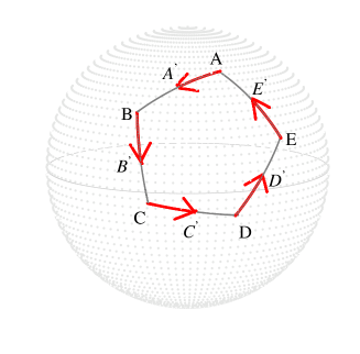
Figure 6: Shown, in the case of a geodesic pentagon on ${\cal P}$, is the connection between Pancharatnam phase and Hamilton’s turns. ${\rm A^{\prime},\;B^{\prime},\,C^{\prime},\;D^{\prime},\;E^{\prime}}$ are the mid-points of the sides of the pentagon ABCDE. On the one hand turns ${\rm AA^{\prime},\;BB^{\prime},\;CC^{\prime},\;DD^{\prime},\;EE^{\prime}}$ evolves or drives the initial state A in an in-phase manner along the five sides of the pentagon, resulting in phase change (Pancharatnam phase) equaling half the area of ABCDE. on the other hand, these turns compose to a turn about A of turn length equaling half the area of ABCDE.

The connection between turns and Pancharatnam or geometric phase emerges quite simply when we combine these two observations. Consider the geodesic pentagon ABCDE of states shown in Fig. 6. Let ${\rm A^{\prime},\;B^{\prime},\;C^{\prime},\;D^{\prime},\;E^{\prime}}$ be the mid points of, respectively, AB, BC, CD, DE, and EA, and let ${\cal A}$ be the area of ABCDE. Starting with the state corresponding to the point A, ${\rm turn~{}AA^{\prime}}$ drives it in an in-phase manner along AB to B, ${\rm turn~{}BB^{\prime}}$ drives B in an in-phase manner along BC to C, ${\rm turn~{}CC^{\prime}}$ drives C to D along CD, ${\rm turn~{}DD^{\prime}}$ drives D to E, and finally ${\rm turn~{}EE^{\prime}}$ drives E back to A along EA in an in-phase manner.

Now this closed-circuit evolution can be viewed from two perspectives. Since the state A is taken along the pentagon ABCDE back to A in an in-phase manner, according to Pancharatnam the final state at A will differ from the initial one by a phase equal to ${\cal A}/2$. From the perspective of Hamilton and his turns, we have that ${\rm turn~{}AA^{\prime}}$, ${\rm turn~{}BB^{\prime}}$, ${\rm turn~{}CC^{\prime}}$, ${\rm turn~{}DD^{\prime}}$, and ${\rm turn~{}EE^{\prime}}$ acting in that sequence have the combined effect of leaving A invariant. That is, A is a fixed point of ${\rm turn~{}AA^{\prime}}+{\rm turn~{}BB^{\prime}}+{\rm turn~{}CC^{\prime}}+{\rm turn~{}DD^{\prime}}+{\rm turn~{}EE^{\prime}}$. However, any turn leaving A invariant should be a turn about $\bm{\hat{n}}_{A}$, the unit vector specified by A $\in{\cal P}$. Since we know from the area formula (61) adapted to the present case that the turn length of this composite turn is ${\cal A}/2$, we conclude

$$T(\bm{\hat{n}}_{A},\,{\cal A}/2)={\rm turn~{}AA^{\prime}}+{\rm turn~{}BB^{\prime}}+{\rm turn~{}CC^{\prime}}$$

$$+{\rm turn~{}DD^{\prime}}+{\rm turn~{}EE^{\prime}},~{}~{}~{}~{}$$ (78)

and this completes the connection between Hamilton’s turns and Pancharatnam’s geometric phase.

Our demonstration has been for the case of a pentagon, but it should be clear that the conclusion generalizes to $n$-sided polygons and, as a suitable limit, to any closed circuit on ${\cal P}$.

VI Elementary exercises in the use of turns

In this section we illustrate the use of turns in several simple situations involving single-qubit gates. The insight developed through these elementary exercises will prove to be of much value in our analysis to be taken up in the next section.

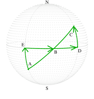
Figure 7: The relationship between the Euler parameters $\xi,\eta,\zeta$ of an SU(2) gate $u(\xi,\,\eta,\,\zeta)$ and the positional spherical coordinates on ${\cal T}$ of the associated turn. The positional coordinates of B, C, A are, respectively, $(\pi/2,\,\varphi_{1}),\,(\theta,\,\varphi_{2}),\,(\pi-\theta,\,2\varphi_{1}-\varphi_{2})$.

Clearly, the first requirement for the effective use of turns as a tool-kit for handling SU(2) gates is an ability to translate freely between the positional coordinates of a turn on the sphere ${\cal T}$ on the one hand and the Euler parameters (angles) of the associated SU(2) matrix on the other. Given an SU(2) gate $u(\xi,\eta,\zeta)$, we slide the representative arc of its turn on its great circle so that the tail (or head) is on the equator. Let the spherical coordinates $(\theta,\varphi)$ of the tail and head of turn BC be, respectively, $(\pi/2,\varphi_{1})$, $(\theta,\varphi_{2})$, as in Fig. 7. It is clear that ${\rm turn~{}BD=turn~{}EB}$ corresponds to optical rotator $R(2\varphi_{2}-2{\varphi}_{1})$, ${\rm turn~{}DC}$ to birefringent plate $C_{-{\pi}/{4}+{\varphi_{2}}/{2}}(\pi-2\theta)$, and ${\rm turn~{}AE}$ to $C_{-{\pi}/{4}+\varphi_{1}-{\varphi_{2}}/{2}}(\pi-2\theta)$. Thus, we have the suggestive resolution of ${\rm turn~{}BC}$ into its ”vertical” (birefringence) and ”horizontal” (optical rotation) parts :

$$u(\xi,\eta,\zeta) \sim {\rm turn}~{}BC\,\,=\,\,{\rm turn}~{}BD\,\,+\,\,{\rm turn}~{}DC$$ (79)

$$= C_{-{\pi}/{4}+{\varphi_{2}}/{2}}(\pi-2\theta)\,R(2\varphi_{2}-2\varphi_{1}).\;\;\;\,$$

In place of this rotation followed by birefringence decomposition we could have equally well considered the birefringence followed by rotation decomposition. Since ${\rm turn~{}AB}={\rm turn~{}BC}$, the positional coordinates of A are $(\pi-\theta,\,2\varphi_{1}-\varphi_{2})$. We have

$$u(\xi,\eta,\zeta) \sim {\rm turn}~{}AB\,\,=\,\,{\rm turn}~{}AE\,\,+\,\,{\rm turn}~{}EB$$ (80)

$$= R(2\varphi_{2}-2\varphi_{1})\,C_{-{\pi}/{4}+\varphi_{1}-{\varphi_{2}}/{2}}(\pi-2\theta).~{}~{}$$

Comparing either of these decompositions with Eq. (22) one readily deduces

$$\xi = -\frac{\pi}{2}+\varphi_{2},$$

$$\eta = \pi-2\theta,$$

$$\zeta = \frac{\pi}{2}+\varphi_{2}-2\varphi_{1},$$ (81)

where $\varphi_{1},\varphi_{2},\theta$ are the positional spherical coordinates of the turn associated with $u(\xi,\eta,\zeta)$.

These are precisely the kind of relationships we were after, and it is significant that these expressions which connect the positional spherical coordinates on ${\cal T}$ of a turn to its Euler angles are linear.

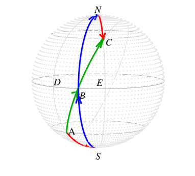
Figure 8: The commutation relation between a QWP and a HWP, yielding the rule for going from the Q-H configuration to the H-Q configuration and vice versa.

Our next exercise concerns the composition of a QWP and a HWP, as shown in Fig. 8. Points D, B, E are on the equator, A and C are on the circles of $45^{\circ}$ latitude, and N, S are the polar points. Let $\varphi_{1}$, $\varphi_{2}$, $\varphi_{3}$ be the azimuthal coordinates of the equatorial points D, B, E and assume DB = BE or, equivalently, $\varphi_{3}=2\varphi_{2}-\varphi_{1}$. It is clear that ${\rm turn~{}AS}$ represents $Q_{\pi/4+\varphi_{1}/2}$ while ${\rm turn~{}NC}$ represents $Q_{{\pi}/{4}+{\varphi_{3}}/2}$. Further, ${\rm turn~{}SB}$ = ${\rm turn~{}BN}$ represents $H_{-{\pi}/{4}+{\varphi_{2}}/{2}}$.

Now consider the pair of spherical triangles ASB, CNB. The angle at N equals the angle at S, in view of the assumption $\varphi_{3}-\varphi_{2}=\varphi_{2}-\varphi_{1}$. Further, AS = CN and SB = NB. Thus, these triangles are congruent, showing that ${\rm turn~{}AB=turn~{}BC}$. In other words,

$${\rm turn~{}AS}+{\rm turn~{}SB} = {\rm turn~{}BN}+{\rm turn~{}NC};$$

that is,

$$H_{-\pi/4+\varphi_{2}/2}Q_{\pi/4+\varphi_{1}/2} = Q_{\pi/4+\varphi_{3}/2}H_{-\pi/4+\varphi_{2}/2},$$ (82)

$${\rm with}~{}\varphi_{1}+\varphi_{3}=2\varphi_{2}.~{}~{}~{}$$

Denoting $\pi/4+\varphi_{1}/2=\varphi$ and $-\pi/4+\varphi_{2}/2=\varphi^{\,{}^{\prime}}$, the constraint $\varphi_{1}+\varphi_{3}=2\varphi_{2}$ is equivalent to $\pi/4+\varphi_{2}/2=2\varphi^{\,{}^{\prime}}-\varphi~{}\;\text{mod}~{}\pi$, and so we have

$$H_{\varphi^{\,{}^{\prime}}}\,Q_{\varphi}=Q_{2\varphi^{\,{}^{\prime}}-\varphi}\,H_{\varphi^{\,{}^{\prime}}},~{}\;\forall\;\varphi,\;\varphi^{\,{}^{\prime}}.$$ (83)

This ”commutation relation” shows that the H-Q configuration cannot have a capability not shared by the Q-H configuration.

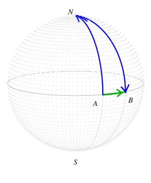
Figure 9: Realization of variable optical rotator using a pair of HWPs. This can also be viewed as depicting the special ability of a HWP to ”absorb” an arbitrary amount of optical rotation.

The composition of a pair of HWPs is our next exercise and this is depicted in Fig. 9. Let $\varphi_{1},\,\varphi_{2}$ be the azimuthal coordinates of the equatorial points A, B. Then ${\rm{turn}~{}AB}=R(2\varphi_{2}-2\varphi_{1})$, ${\rm turn~{}SA}={\rm turn~{}AN}=H_{-\pi/4+\varphi_{1}/2}$, and ${\rm turn~{}NB}={\rm turn~{}BS}=H_{\pi/4+\varphi_{2}/2}$. One readily reads out from Fig. 9

$$\rm{turn}~{}AB =\rm{turn}~{}AN+\rm{turn}~{}NB$$

$$\text{that is, }~{}~{}R(2\varphi_{2}-2\varphi_{1}) =H_{\pi/4+\varphi_{2}/2}\,H_{-\pi/4+\varphi_{1}/2}.$$ (84)

With $\pi/4+\varphi_{2}/2\equiv\varphi$ and $-\pi/4+\varphi_{1}/2\equiv\varphi^{\,{}^{\prime}}$ we have

$$H_{\varphi}\,H_{\varphi^{\,{}^{\prime}}}=R(2\pi+4(\varphi-\varphi^{\,{}^{\prime}})).$$ (85)

Recall from Eq. (20) that it is $R(4\pi)$, and not $R(2\pi)$, that equals the SU(2) identity $\tau_{0}$. [Indeed, $R(2\pi)=-\tau_{0}$.] Noting that $H_{\pm\pi/2+\varphi}$ is the inverse of $H_{\varphi}$, we may rewrite the last identity in the form

$$H_{\varphi}\,H_{\pm\pi/2+\varphi^{\,{}^{\prime}}}=R(\,4(\varphi-\varphi^{\,{}^{\prime}})\,).$$ (86)

The preceding identity [Eq. (86)] shows that a variable optical rotator can be simply realized with a pair of HWPs, the effective rotation or optical activity being linear in the relative orientation (of the fast axis) of the HWPs.

There is another instructive and important manner in which Fig. 9 can be read. Since $\rm{turn~{}BN}$ corresponds to $H_{-\pi/4+\varphi_{2}/2}$, the fact that $\rm{turn~{}AN}=\rm{turn~{}AB}+\rm{turn~{}BN}$ reads $H_{-\pi/4+\varphi_{1}/2}=H_{-\pi/4+\varphi_{2}/2}\,R(2\varphi_{2}-2\varphi_{1})$, or $H_{\varphi}\,R(\alpha)=H_{\varphi-\alpha/4}$. Similarly, the visual identity $\rm{turn~{}SA}+\rm{turn~{}AB}=\rm{turn~{}SB}$ reads $R(2\varphi_{2}-2\varphi_{1})\,H_{-\pi/4+\varphi_{1}/2}=H_{-\pi/4+\varphi_{2}/2}$. We have thus proved

$$R(\alpha)\,H_{\varphi}=H_{\varphi+\alpha/4},\,~{}~{}H_{\varphi}\,R(\alpha)=H_{\varphi-\alpha/4}.$$ (87)

These two identities are equivalent to, and consistent with, one another in view of the defining property $R(\alpha)\,H_{\varphi}\,R(-\alpha)=\Phi(\alpha/2)\,H_{\varphi}\,\Phi(-\alpha/2)=H_{\varphi+\alpha/2}$ of $R(\alpha)$, and they exhibit the special capability of a HWP to ‘absorb’ optical rotation and still remain a HWP. This absorption property, combined with the earlier noted property that a pair of HWPs is simply equivalent to an optical rotator, implies that three HWPs can fare no better than one HWP.

Our last result shows that any number of HWPs cannot, by themselves, realize much portion of the manifold of SU(2) gates; indeed, an odd number of them is no better than just one HWP, while an even number is simply equivalent to a (variable) optical rotator. In either case, not more than a one-parameter family of SU(2) gates gets realized.

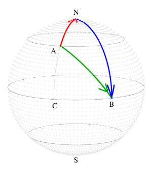
Figure 10: The subset of unitary gates that can be realized with one QWP and one HWP. Shown also is the fact that addition of a second HWP can not in any manner enlarge this subset.

One is thus led to ask how much portion of the SU(2) manifold of unitary gates can be realized with two HWPs and one QWP. Let us begin with just one HWP and one QWP, as shown in Fig. 10, where the point A lies on the $45^{\circ}$ latitude circle, and B and C on the equator. Let $\varphi_{1}$ be the azimuthal coordinate of A and C and $\varphi_{2}$ that of B. Then $\rm{turn~{}AN}$ corresponds to $Q_{-\pi/4+\varphi_{1}/2}$ and $\rm{turn~{}NB}$ to $H_{\pi/4+\varphi_{2}/2}$. As a consequence of the visual identity $\rm{turn~{}AB}=\rm{turn~{}AN}+\rm{turn~{}NB}$ we deduce that ${\rm turn~{}AB}$ corresponds to $H_{\pi/4+\varphi_{2}/2}Q_{-\pi/4+\varphi_{1}/2}$. It follows that the turns or SU(2) gates realizable with one HWP and one QWP are distinguished by the property that such turns extend from one of the $45^{\circ}$ latitude circles to the equator or, equivalently, from the equator to a $45^{\circ}$ latitude circle.

However, from the identity $\rm{turn~{}AB}=\rm{turn~{}AC}+\rm{turn~{}CB}$ we see that such a turn is equivalent to a QWP followed by an optical rotator. Since an optical rotator and a pair of HWPs are equivalent, we conclude that turns realizable by two HWPs and one QWP are certainly of the same form as $\rm{turn~{}AB}$, that is, extending between a $45^{\circ}$ latitude circle and the equatorial circle. Since such turns are fully parametrized by their azimuthal coordinates on these two circles, we conclude that two HWPs and one QWP can realize only a two-parameter family of SU(2) gates, and that this family is precisely the one realized using one QWP and just one HWP.

It turns out that with two QWPs and one HWP one can realize the entire SU(2) manifold of unitary gates [that three QWPs by themselves will not suffice is readily seen from the fact that they cannot realize, for instance, any SU(2) element whose turn has length $>3\pi/4$]. Before we turn to the next section for proof of this claim of three component realization of all SU(2) gates we examine, as our last exercise in this section, the manner in which a pair of QWPs transform a variable optical rotator into a variable birefringent plate.

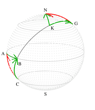
Figure 11: Diagram showing that a pair of QWPs can convert variable optical rotation into variable birefringence.

The points $\rm{C,\,G}$ of Fig. 11 are on the $45^{\circ}$ latitude circles and points ${\rm A,\,B}$ are on the equator. Let ${\rm AB}=\eta/2$. Point ${\rm K}$ on the geodesic ${\rm CBG}$ is so chosen that ${\rm CB=KG}$. It is clear that $\rm{turn~{}GN}$ corresponds to QWP $Q_{0}$, $\rm{turn~{}CA}$ to its inverse, $Q_{\pi/2}$, and $\rm{turn~{}AB}$ to $R(\eta)$.

Let us now consider the pair of spherical triangles ${\rm CAB,\,GNK}$. We have ${\rm AC=NG}$, angle at ${\rm C}=$ angle at ${\rm G}$, while ${\rm CB=KG}$ by construction. Thus, the triangles are congruent. This means, on the one hand, that angle at ${\rm N}=$ angle at ${\rm A=}~{}\pi/2$ so that $\rm{turn~{}KN}$ is a birefringent plate $C_{-\pi/4}(\cdot)$ and, on the other hand, that $\rm{KN=AB=}~{}\eta/2$, so that $\rm{turn~{}KN}$ corresponds to $C_{-\pi/4}(\eta)$. We have thus established

$$\rm{turn}~{}KN =\rm{turn}~{}KG+\rm{turn}~{}GN$$

$$=\rm{turn}~{}CB+\rm{turn}~{}GN$$

$$=\rm{turn}~{}CA+\rm{turn}~{}AB+\rm{turn}~{}GN\,;$$

$$\text{that is, }~{}~{}~{}C_{-\pi/4}(\eta) =Q_{0}\,R(\eta)\,Q_{\pi/2}.$$ (88)

Conjugating by $\Phi(\pi/4)$ we have $C_{0}(\eta)=Q_{\pi/4}\,R(\eta)\,Q_{-\pi/4}$, which on conjugation by $\Phi(\varphi)$ yields

$$C_{\varphi}(\eta)=Q_{\pi/4+\varphi}\,R(\eta)\,Q_{-\pi/4+\varphi}.$$ (89)

This relationship between variable optical rotation and variable birefringence is what we set out to demonstrate. However, to the extent that the variable optical rotator is not a preferred component, the fact remains that this may not be the most convenient way to realize variable birefringence.

VII Realization of all SU(2) gates Using Two QWPs and one HWP

Since HWP and QWP have each only one (rotational) degree of freedom, and since SU(2) is a 3-parameter manifold, it is clear that at least three components are required to realize even a small nontrivial (nonzero measure) part of this manifold. We have already noted that one QWP and two HWPs cannot fare any better than a QWP plus a HWP. In the present section we prove, using insights developed through the elementary exercises of the last section, that two QWPs and one HWP are sufficient to realize the full group manifold of SU(2) gates.

The proof is straight-forward and relies entirely on Fig. 12. The points A, B, D are on the equator, N and S are the polar points, and C, G are on the circles of 45^∘ latitude. The point F, the intersection of line (great circle arc) DN with line CBG, is not assumed to be on the circle of 45^∘ latitude; the fact that F indeed lies on this circle will emerge by itself. The point K on the line CBG is so chosen that turn CB = turn KG. We do not assume that the angle GNK equals $\pi/2$. The fact that NK and NG are orthogonal at N will unfold on its own; turn KN will then correspond to a birefringent plate $C_{-\pi/4}(\eta^{\,{}^{\prime}})$, where $\eta^{\,{}^{\prime}}$ equals twice the arclength of KN. It is this turn corresponding to variable birefringence that will eventually become the focus of our attention.

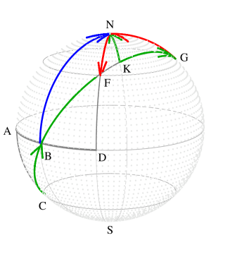
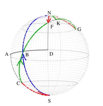
Figure 12: Realization of all SU(2) gates using just two QWPs and one HWP. Two perspectives are presented for visual convenience.

We assume ${\rm AB}={\rm BD}=\eta/2$. Our first task is to prove that the point F lies on the 45^∘ latitude circle. We begin by noting that turn GN corresponds to QWP $Q_{0}$ and so is also turn CS.

Consider the pair of spherical triangles ABC, DBF. The angle at A equals the angle at D (both equal $\pi/2$). Both triangles have the same angle at B, and AB = BD by construction. Thus, the two triangles are congruent. It follows that DF= AC = $\pi/4$, showing that F lies indeed on the 45^∘ latitude circle, and that turn BF = turn CB. Since F is on the 45^∘ latitude circle, turn NF corresponds to QWP $Q_{\eta/2}$. Since AB = $\eta/2$, turn BN = turn SB corresponds to HWP $H_{\pi/2+\eta/4}=H_{-\pi/2+\eta/4}$.

Now consider the pair of spherical triangles ABC, KNG. The angle at C obviously equals the angle at G. Further, CB = KG by construction and AC = GN (= $\pi/4$), showing that the two triangles are congruent. As one consequence we see that the angle at N is $\pi/2$, showing that turn NK is indeed the birefringent plate $C_{-\pi/4}(\,\cdot\,)$. As another consequence we have KN = AB = BD = $\eta/2$, showing that turn KN = $C_{-\pi/4}(\eta)$. But, in a visually obvious manner,

$${\rm turn~{}KN} = {\rm turn~{}KG}+{\rm turn~{}GN}$$ (90)

$$= {\rm turn~{}BF}+{\rm turn~{}GN}$$

$$= {\rm turn~{}BN}+{\rm turn~{}NF}+{\rm turn~{}GN}.\;\;$$

Since turn KN = $C_{-\pi/4}(\eta)$, and since the three turns on the right-hand side of the last equation equal, respectively, $H_{\pi/2+\eta/4}$, $Q_{\eta/2}$, and $Q_{0}$, we have proved

$$C_{-\pi/4}(\eta)=Q_{0}\,Q_{\eta/2}\,H_{\pi/2+\eta/4},$$ (91)

demonstrating the realizability of variable birefringence. We see from Fig. 12 that turn KN could have also been developed in a somewhat different but equivalent manner:

$${\rm turn~{}KN} = {\rm turn~{}KG}+{\rm turn~{}GN}$$ (92)

$$= {\rm turn~{}CB}+{\rm turn~{}GN}$$

$$= {\rm turn~{}CS}+{\rm turn~{}SB}+{\rm turn~{}GN}.\;\;$$

It is clear that this corresponds to the multiplicative identity

$$C_{-\pi/4}(\eta)=Q_{0}\,H_{\pi/2+\eta/4}\,Q_{0}.$$ (93)

Incidentally, the fact that these two realizations of $C_{-\pi/4}(\eta)$ respectively in the Q-Q-H and Q-H-Q configurations are equivalent can also be verified using the H-Q commutation relation in Eq. (83).

Conjugating Eq. (91) by $\Phi(\pi/4)$, which corresponds to rigidly rotating Fig. 12 by $\pi/2$ about the polar axis, we have

$$C_{0}(\eta)=Q_{\pi/4}\,Q_{\pi/4+\eta/2}\,H_{-\pi/4+\eta/4},$$ (94)

a variable birefringent plate with the fast polarization along the $x_{1}$ axis. The reader will appreciate that Fig. 12 was crafted for $C_{-\pi/4}(\eta)$ rather than $C_{0}(\eta)$ simply for visual clarity.

Conjugating the last equation by $\Phi(\xi/2)$, which amounts to a further rigid rotation of Fig. 12 by $\xi$ about the polar axis, one obtains

$$C_{\xi/2}(\eta)=Q_{\pi/4+\xi/2}\,Q_{\pi/4+\xi/2+\eta/2}\,H_{-\pi/4+\xi/2+\eta/4}.\;\;$$ (95)

Right multiplying by the optical rotator $R(\xi+\zeta)$, and using the special ability of HWP to ”absorb” rotation, namely $H_{(\cdot)}R(\alpha)=H_{(\cdot)-\alpha/4}$, we have in view of $u(\xi,\,\eta,\,\zeta)=C_{\xi/2}(\eta)R(\xi+\zeta)$ given in Eq. (22)

$$u(\xi,\,\eta,\,\zeta)=Q_{\pi/4+\xi/2}\,Q_{\pi/4+\xi/2+\eta/2}\,H_{-\pi/4+(\xi+\eta-\zeta)/4},\;\,$$

showing that all SU(2) gates can be realized using two QWPs and one HWP in the Q-Q-H configuration. Uniqueness of this realization as well as the fact that the required (angular) positions of the plates are linear in the Euler angles should be appreciated.

That a similar assertion holds for the other two possible configurations, namely, Q-H-Q and H-Q-Q, follows immediately from the Q-H commutation relation $Q_{\alpha}H_{\beta}=H_{\beta}Q_{2\beta-\alpha}$ of Eq. (83):

$$u(\xi,\,\eta,\,\zeta)=Q_{\pi/4+\xi/2}\,H_{-\pi/4+(\xi+\eta-\zeta)/4}\,Q_{\pi/4-\zeta/2};\;\;\,$$ (97)

$$u(\xi,\,\eta,\,\zeta)=H_{-\pi/4+(\xi+\eta-\zeta)/4}\,Q_{\pi/4+(\eta-\zeta)/2}\,Q_{\pi/4-\zeta/2}.$$

We have thus completed a proof of the main result of this section, indeed this paper:

Theorem: All SU(2) gates $u(\xi,\,\eta,\,\zeta)$ can be realized with just two QWPs and one HWP equally well in any one of the three conceivable configurations Q-Q-H, Q-H-Q, or H-Q-Q, as detailed, respectively, in Eqs. (VII), (97), and (VII). The realization is unique in each case, and in each configuration the angular positions of the plates are linear in the Euler angles $\xi,\,\eta,\,\zeta$ of the gate.

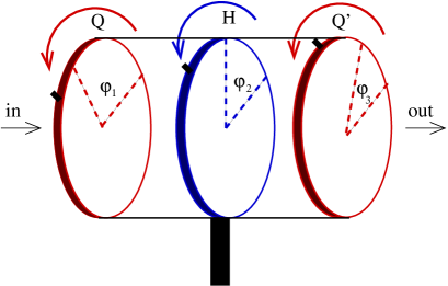
Figure 13: The assembly of the universal gadget which realizes all single-qubit unitary gates. The three wave plates Q, H, Q’ are coaxialy mounted, with a provision being made to assign and read the orientations of their fast axes any triplet of values.

VIII Universal single-qubit unitary gate

The theorem proved above enables assembling of a universal single-qubit unitary gate as described below. While the universal gate can be assembled in any one of the three configurations Q-Q-H, Q-H-Q, or H-Q-Q we choose the configuration Q-H-Q simply in order to be concrete.

Let two QWPs Q, Q${}^{\,{}^{\prime}}$ and a HWP H be coaxially mounted in a cylindrical case, as shown in Fig. 13. Assume that a provision is made to rotate each one of the three plates Q, H, Q${}^{\,{}^{\prime}}$ independently about the axis of the cylinder, and that provision is made to read out the angular coordinates $\varphi_{1},\;\varphi_{2},\;\varphi_{3}$ of their fast axes on their respective (semicircular) dials. We assume further that the assembly is so used that light passes through Q, H, Q${}^{\,{}^{\prime}}$ in that order.

Clearly, the SU(2) matrix corresponding to the entire assembly is $Q^{\,{}^{\prime}}_{\varphi_{3}}\,H_{\varphi_{2}}\,Q_{\varphi_{1}}$. Thus, to realize any unitary gate $u(\xi,\,\eta,\,\zeta)\in~{}$SU(2) we have to simply arrange these dial positions to read

$$\varphi_{1} = \pi/4-\zeta/2~{}~{}{\rm mod}\;\pi,$$

$$\varphi_{2} = -\pi/4+(\xi+\eta-\zeta)/4~{}~{}{\rm mod}\;\pi,$$

$$\varphi_{3} = \pi/4+\xi/2~{}~{}{\rm mod}\;\pi,$$ (99)

as may be seen from Eq. (97).

That the entire SU(2) manifold of unitary gates can be realized using a single assembly has its advantages. For instance, if the only imperfections of the wave plates from ideal ones are residual losses, the fact that the total loss of the assembly is the same for realization of every SU(2) gate, independent of the Euler angles $(\xi,\eta,\zeta)$ of the gate, implies that it can be accounted for more easily. Further, the fact that the dynamical phase through the system remains the same for all gates can prove to be of particular importance in interference considerations, particularly in the context of geometric phase experiments kimble1 ; mandel .

IX Concluding Remarks

In this paper we have developed in considerable detail the pictorial construction of Hamilton into a tool-kit for handling problems of synthesis and analysis in situations where the unitary group SU(2) plays a central role. This group pervades nearly all areas of science, either directly or through its cousin SO(3). Thus, this tool-kit should be of interest to a wider audience beyond quantum computation and quantum information. [In particular, the formalism and results presented here should be of much interest to classical polarization optics.] It is for this reason that we have developed Hamilton’s construction itself in sufficient detail, taking care to bring out its connection with geometric phase and the Bargmann invariants. It is in view of this detailed preparation that we believe the manipulations with turns presented in Sections 6, 7, and 8 will be found to be fully accessible to a broad spectrum of readership.

As noted in the Introduction, the central result presented as a theorem towards the end of the paper is not new in itself. Our presentation is fashioned to work toward this result for two reasons. First, to demonstrate how this geometric approach is suggestive and visually transparent compared to the algebraic approach. Second, this result acts as a focal point in the sense that in working towards it most of the simple manipulations with turns are conveniently developed and demonstrated in stages.

It is true that all the results developed here geometrically could be algebraically verified through matrix multiplication. However, it is in the geometric representation that synthesis results suggest themselves in a vivid or visual manner. We may cite the H-Q commutation relation in Fig. 8 and the ”absorption” of optical rotation by a HWP (as also the realization of variable optical rotator using a pair of HWPs) in Fig. 9 as effective illustrations of this advantage.

Finally, our presentation of turns in this paper is in the context of the unitary group SU(2). The reader will easily realize that this geometric representation readily translates to the rotation group SO(3) if a turn of length $\ell$ and the reversed turn of length $\pi-\ell$ are identified. This amounts to identifying the null turn with the turn of length $\pi$, which is clearly the same thing as identifying $U$ of SU(2) with $-\,U$ of SU(2). Thus, the turn length $\ell$ in the case of SO(3) gets restricted to the range $0\leq\ell\leq\pi/2$.

Acknowledgement: The authors would like to thank Professor N. Mukunda for a critical reading of the manuscript.

References

- (1) E.H. O’Neil, Introduction to Statistical Optics (Addison-Wesley Reading, MA, 1981).
- (2) E. Wolf, Introduction to the Theory of Coherence and Polarization of Light (Cambridge University Press, Cambridge, UK, 2007).
- (3) E.B. Davis, Quantum Theory of Open systems (Academic Press, NY, 1976).
- (4) W.R. Hamilton, Lectures on Quaternions (Hodges and Smith, Dublin, 1853).
- (5) L.C. Biedenharn and L.D. Louck, Angular Momentum in Quantum Physics: Theory and Applications, Vol. 8 of the Series “Encyclopedia of Mathematics and its Applications” (Addison-Wesley, NY, 1981).
- (6) N. Mukunda, S. Chaturvedi, and R. Simon, Pramana—Jour. Phys. 74, 1 (2010).
- (7) R. Simon, N. Mukunda and E.C.G. Sudarshan, Pramana—J. Phys. 32, 769 (1989).
- (8) R. Simon, N. Mukunda and E.C.G. Sudarshan, Phys. Rev. Lett. 62, 1331 (1989).
- (9) R. Simon, N. Mukunda, and E.C.G. Sudarshan, Jour. Math. Phys. 30, 1000 (1989).
- (10) M. Juarez and M. Santander, Jour. Phys. A: Math. Gen. 15, 3411 (1982).
- (11) R. Simon, S. Chaturvedi, V. Srinivasan, and N. Mukunda, Int. Jour. Theor. Phys. 45, 2075 (2006).
- (12) E. Knill, R. Laflamme, and G.J. Milburn, Nature (London) 409, 46 (2001).
- (13) P. Kok, W.J. Munro, K. Nemoto, T.C. Ralph, J.P. Dowling, and G.J. Milburn, Rev. Mod. Phys. 79, 135 (2007).
- (14) H.J. Kimble, Nature 453, 1023 (2008).
- (15) M. Nielsen and I. Chuang, Quantum Computation and Quantum Information (Cambridge Univ. Press, Cambridge, 2000).
- (16) D. Deutsch, A. Barenco, and A. Ekert, Proc. Roy. Soc. Lond. A 449, 669 (1995).
- (17) A. Barenco, C.H. Bennett, R. Cleve, D.P. DiVincenzo, N. Margolus, P.W. Shor, T. Sleator, J.A. Smolin, and H. Weinfurter, Phys. Rev. A 52, 3457 (1995).
- (18) D.P. DiVincenzo, Proc. Roy. Soc. Lond. A 454, 261 (1998).
- (19) R. Simon and N. Mukunda, Phys. Lett. A 143, 165 (1990).
- (20) V. Bagini, R. Borghi, F. Gori, M. Santarsiero, F. Frezza, G. Schettini, and G.S. Spagnolo, Eur. Jour. Phys. 17, 279 (1996).
- (21) U. Gopinathan, T.J. Naughton, and J.T. Sheridan, Appl. Opt. 45, 5693 (2006).
- (22) J.C. Loredo, O. Ortiz, R. Weingärtner, and F. De Zela, Phys. Rev. A 80, 012113 (2009).
- (23) Arvind, G. Kaur, G. Narang, Jour. Opt. Soc. Am. B 24, 221 (2007).
- (24) E. Karimi, S. Slussarenko, B. Piccirillo, L. Marrucci, and E. Santamato, Phys. Rev. A 81, 053813 (2010).
- (25) M. Haynen and J.P. Thayer, Jour of Atmospheric and Solar-Terrestrial Physics 73, 2110 (2011).
- (26) L. Ainola and H. Aben, Jour. Opt. Soc. Am. A 24, 3397 (2007).
- (27) S.T. Tang and H.S. Kwok, Jour. Opt. Soc. Am. A 18, 2138 (2001).
- (28) R. Bhandari, Phys. Lett. A 138, 469 (1989).
- (29) R. Simon and N. Mukunda, Phys. Lett. A 138, 474 (1989).
- (30) R.A. Campos, B.E.A. Saleh, and M.C. Teich, Phys. Rev. A 40, 1371 (1989).
- (31) R. Simon and N. Mukunda, J. Phys. A: Math. Gen. 25, 6135 (1992).
- (32) M.V. Berry, Proc. Roy. Soc. A 392, 45 (1984).
- (33) S. Pancharatnam, Proc. Iadian Acad. Sci. A 44, 247 (1956).
- (34) S. Ramaseshan and R. Nityananda, Curr. Sci. 55, 1225 (1986).
- (35) M. V. Berry, Jour. Mod. Opt. 34, 1401 (1987).
- (36) V. Bargmann, J. Math. Phys. 5, 862 (1964).
- (37) N. Mukunda and R. Simon, Ann. Phys. 228, 205 (1993).
- (38) N. Mukunda and R. Simon, Ann. Phys. 228, 269 (1993).
- (39) R. Simon and N. Mukunda, Phys. Rev. Lett. 70 , 880 (1993).
- (40) E.M. Rabei, Arvind, N. Mukunda, and R. Simon, Phys. Rev. A 60, 3397 (1999).
- (41) N. Mukunda, Arvind, S. Chaturvedi, and R. Simon, Phys. Rev. A 65, 012102 (2002).
- (42) N. Mukunda, Arvind, E. Ercolessi, G. Marmo, G. Morandi, and R. Simon, Phys. Rev. A 67, 042114 (2003).
- (43) N. Mukunda, P.K. Arvind, and R. Simon, Jour. Phys. A: Math. Gen. 36, 2347 (2003).
- (44) T.H. Chyba, L.J. Wang, L. Mandel and R. Simon, Opt. Lett. 13, 562 (1988).
- (45) R. Simon, H.J. Kimble and E.C.G. Sudarshan, Phys. Rev. Lett. 61, 19 (1988).