Robust Image Analysis by $L_{1}$-Norm Semi-supervised Learning

Abstract

This paper presents a novel $L_{1}$-norm semi-supervised learning algorithm for robust image analysis by giving new $L_{1}$-norm formulation of Laplacian regularization which is the key step of graph-based semi-supervised learning. Since our $L_{1}$-norm Laplacian regularization is defined directly over the eigenvectors of the normalized Laplacian matrix, we successfully formulate semi-supervised learning as an $L_{1}$-norm linear reconstruction problem which can be effectively solved with sparse coding. By working with only a small subset of eigenvectors, we further develop a fast sparse coding algorithm for our $L_{1}$-norm semi-supervised learning. Due to the sparsity induced by sparse coding, the proposed algorithm can deal with the noise in the data to some extent and thus has important applications to robust image analysis, such as noise-robust image classification and noise reduction for visual and textual bag-of-words (BOW) models. In particular, this paper is the first attempt to obtain robust image representation by sparse co-refinement of visual and textual BOW models. The experimental results have shown the promising performance of the proposed algorithm.

I Introduction

Semi-supervised learning, i.e., learning from both labeled and unlabeled data, has been widely applied to many challenging image analysis tasks [1, 2, 3, 4, 5, 6] such as image representation, image classification, and image annotation. In different image analysis tasks, the manual labeling of training data is often tedious, subjective as well as expensive, while the access to unlabeled data is much easier. Through exploiting the large number of unlabeled data with reasonable assumptions, semi-supervised learning [7, 8, 9, 10, 11] can reduce the need for expensive labeled data and thus achieve promising results especially for community-contributed image collections (e.g. Flickr).

Among various semi-supervised learning methods, one influential work is graph-based semi-supervised learning [8, 9] which models the entire dataset as a graph. The basic idea behind this semi-supervised learning is label propagation on the graph with the cluster consistency [9] (i.e. two data points on the same geometric structure are likely to have the same class label). Since the graph is at the heart of graph-based semi-supervised learning, graph construction has been extensively studied [12, 13, 14, 15] in the past years. However, these graph construction methods are not developed directly for noise reduction, and the corresponding semi-supervised learning may suffer from significant performance degradation due to the inaccurate labeling of data points commonly encountered in different image analysis tasks. For example, the annotations of images may be contributed by the community (see Flickr) and we can only obtain noisy tags.

In this paper, we focus on proposing a novel noise-robust graph-based semi-supervised learning method, rather than the well-studied graph construction. As summarized in [12], the traditional graph-based semi-supervised learning can be formulated as a quadratic optimization problem based on Laplacian regularization [8, 9, 11, 16, 4]. Considering that the sparsity induced by $L_{1}$-norm optimization can help to deal with the noise in the data to some extent [17, 18], if we succeed in formulating Laplacian regularization as an $L_{1}$-norm term instead, we can convert the traditional semi-supervised learning to $L_{1}$-norm optimization and enable our new semi-supervised learning also to benefit from the nice property of sparsity. Fortunately, derived from the eigenvalue decomposition of the normalized Laplacian matrix $\mathcal{L}$, we can readily represent $\mathcal{L}$ in a symmetrical decomposition form, which can be further used to formulate Laplacian regularization as an $L_{1}$-norm term. Since all the eigenvectors of $\mathcal{L}$ are explored in this symmetrical decomposition, our new $L_{1}$-norm Laplacian regularization can be considered to be explicitly formulated based upon the manifold structure of the data.

As a convex optimization problem, the above $L_{1}$-norm semi-supervised learning has a unique global solution. By working only with a small subset of eigenvectors, we develop a fast sparse coding algorithm for our $L_{1}$-norm semi-supervised learning. In this paper, we only adopt the fast iterative shrinkage-thresholding method [19] for sparse coding, regardless of many other $L_{1}$-norm optimization methods[20, 21, 22, 23]. Due to the nice property of sparsity, the proposed algorithm can deal with the noise in the data to some extent, as shown in our later experiments. Hence, it has important applications to robust image analysis where noisy labels are provided. In this paper, we apply the proposed algorithm to two typical image analysis tasks, i.e., noise-robust semi-supervised image classification and noise reduction for both visual and textual bag-of-words (BOW) models. Although only tested in these two applications, the proposed algorithm can be extended to other image analysis tasks, given that semi-supervised learning has been widely used in the literature.

To emphasize the main contributions of this paper, we summarize the following distinct advantages of our novel $L_{1}$-norm semi-supervised learning:

• We have made the first attempt to formulate Laplacian regularization as an $L_{1}$-norm term explicitly based upon the manifold structure of the data.

• Our $L_{1}$-norm semi-supervised learning algorithm has been shown to achieve significant improvements in robust image analysis where noisy labels are provided.

• Our new $L_{1}$-norm Laplacian regularization can be similarly applied to many other difficult problems, considering the wide use of Laplacian regularization.

• This is the first attempt to obtain robust image representation by sparse co-refinement of visual and textual BOW models for community-contributed image collections.

The remainder of this paper is organized as follows. Section II provides a brief review of related work. In Section III, we propose a fast $L_{1}$-norm semi-supervised learning algorithm by defining novel $L_{1}$-norm Laplacian regularization. In Section IV, the proposed algorithm is applied to two robust image analysis tasks: noise-robust image classification and sparse co-refinement of visual and textual BOW models. In Section V, we present the experimental results to evaluate the proposed algorithm. Finally, Section VI gives the conclusions.

II Related Work

In this paper, we make attempt to formulate graph-based semi-supervised learning as $L_{1}$-norm optimization so that it can benefit from the nice property of sparsity and thus deal with the noise in the data to some extent. This is quite different from the attempt to construct a graph with sparse representation [13, 5, 14] for graph-based semi-supervised learning. Although these two different attempts both exploit $L_{1}$-norm optimization for semi-supervised learning, a new $L_{1}$-norm semi-supervised learning method is proposed in the present paper while the traditional semi-supervised learning was still used in [13, 5, 14]. In fact, the graph constructed with sparse representation can be readily applied to our new $L_{1}$-norm semi-supervised learning algorithm.

To formulate semi-supervised learning as an $L_{1}$-norm optimization problem, we give new $L_{1}$-norm explanation of Laplacian regularization explicitly based upon the manifold structure of the data. This $L_{1}$-norm Laplacian regularization distinguishes our semi-supervised learning algorithm greatly from another $L_{1}$-norm semi-supervised learning algorithm proposed in [24] which directly adopts Lasso [25] for semi-supervised learning and completely ignores the important Laplacian regularization that has been widely used for graph-based semi-supervised learning in the literature [8, 9, 11, 16, 4]. In fact, our $L_{1}$-norm semi-supervised learning algorithm has been shown to outperform [24] significantly (see later experimental results). Moreover, although both Laplacian regularization and $L_{1}$-norm optimization have also been used in [26, 5], the Laplacian regularization term in the objective function is still quadratic, which is quite different from our new $L_{1}$-norm Laplacian regularization.

Since our new $L_{1}$-norm Laplacian regularization is defined directly over the eigenvectors of the normalized Laplacian matrix, we can formulate semi-supervised learning as an $L_{1}$-norm linear reconstruction problem in the framework of sparse coding [17, 18]. Moreover, by working with only a small subset of eigenvectors, we can develop a fast sparse coding algorithm for our $L_{1}$-norm semi-supervised learning, which is efficient even for robust image analysis tasks where the datasets are often large. Although there exist other $L_{1}$-norm generalizations [27, 28] of Laplacian regularization, they are not defined based upon the eigenvectors and the corresponding sparse coding algorithms incur too large time cost.

Considering the distinct advantage (i.e. noise robustness as shown in later experiments) of our $L_{1}$-norm semi-supervised learning, our original motivation is to apply it to robust image analysis where noisy labels are provided. In particular, to our best knowledge, we have made the first attempt to obtain robust image representation by sparse co-refinement of visual and textual BOW models. This strategy is extremely important for the success of robust image analysis on community-contributed image collections (e.g. Flickr), because it becomes rather difficult to generate accurate visual vocabularies and obtain clean image tags in such complicated case. However, in the literature, most previous methods can not deal with visual and textual BOW refinement simultaneously. For example, various supervised [29, 30] and unsupervised [31, 32] methods have been developed specially for visual vocabulary optimization, while in [33, 34, 5] only tag refinement is considered for robust image analysis. More detailed comparison to these methods can be found in Section IV-B.

III $L_{1}$-Norm Semi-Supervised Learning

In this section, we first give a brief review of graph-based semi-supervised learning. To address the problem associated with this semi-supervised learning, we further present new $L_{1}$-norm formulation of Laplacian regularization. Finally, based on this $L_{1}$-norm Laplacian regularization, we develop a fast $L_{1}$-norm semi-supervised learning algorithm.

III-A Graph-Based Semi-Supervised Learning

To introduce graph-based semi-supervised learning, we first formulate a semi-supervised learning problem as follows. Here, we only consider the two-class problem, while the multi-class problem can be handled the same as [9]. Given a dataset $\mathcal{X}=\{x_{1},...,x_{l},x_{l+1},...,x_{n}\}$ and a label set $\{1,-1\}$, the first $l$ data points $x_{i}~{}(i\leq l)$ are labeled as $y_{i}\in\{1,-1\}$ and the remaining data points $x_{u}~{}(l+1\leq u\leq n)$ are unlabeled with $y_{u}=0$. The goal of semi-supervised learning is to predict the labels of the unlabeled data points, i.e., to find a vector $\mathbf{f}=[f_{1},...,f_{n}]^{T}$ corresponding to a classification on the dataset $\mathcal{X}$ by labeling each data point $x_{i}$ with a label $\mathrm{sign}(f_{i})$, where $\mathrm{sign}(\cdot)$ denotes the sign function. Let $\mathbf{y}=[y_{1},...,y_{n}]^{T}$, and we can readily observe that $\mathbf{y}$ is exactly consistent with the initial labels according to the decision rule.

Figure 1: (a) The two-moons toy dataset with each class having one incorrectly (out of five) labeled data point initially. (b) The classification results on this toy dataset by one typical graph-based semi-supervised learning method proposed in [9]. We can clearly observe the severe problem of noise diffusion associated with the traditional semi-supervised learning when noisy initial labels are provided.

To solve the above problem by graph-based semi-supervised learning, we need to model the whole dataset as a graph $\mathcal{G}=\{\mathcal{V},W\}$ with its vertex set $\mathcal{V}=\mathcal{X}$ and weight matrix $W=[w_{ij}]_{n\times n}$, where $w_{ij}$ denotes the similarity between $x_{i}$ and $x_{j}$. The weight matrix $W$ is assumed to be nonnegative and symmetric. For example, we usually define $W$ as

$$w_{ij}=\exp(-||x_{i}-x_{j}||^{2}/(2\sigma^{2})),$$ (1)

where the variance $\sigma$ is a free parameter that can be determined empirically. Moreover, to eliminate the need to tune this parameter, we can adopt the graph construction methods reported in [12, 13, 14]. Based on the weight matrix $W$, we compute the normalized Laplacian matrix $\mathcal{L}$ of the graph $\mathcal{G}$ by

$$\mathcal{L}=I-D^{-\frac{1}{2}}WD^{-\frac{1}{2}},$$ (2)

where $I$ is an $n\times n$ identity matrix, and $D$ is an $n\times n$ diagonal matrix with its $i$-th diagonal element being equal to the sum of the $i$-th row of $W$ (i.e. $\sum_{j}w_{ij}$).

In this paper, we focus on one typical graph-based semi-supervised learning method proposed in [9]. Its objective function can be defined as follows:

$$Q(\mathbf{f})=\frac{1}{2}||\mathbf{f}-\mathbf{y}||_{2}^{2}+\frac{\lambda}{2}\mathbf{f}^{T}\mathcal{L}\mathbf{f},$$ (3)

where $\lambda>0$ is a regularization parameter. Then the classification function is given by

$$\mathbf{f}^{*}=\arg\min_{\mathbf{f}}Q(\mathbf{f}).$$ (4)

The first term of $Q(\mathbf{f})$ is the fitting constraint, which means a good classification function should not change too much from the initial label assignment. The second term is the smoothness constraint, which means that a good classification function should not change too much between nearby data points. The trade-off between these two competitive constraints is captured by the positive parameter $\lambda$. It should be noted that the smoothness constraint actually denotes the well-known Laplacian regularization [8, 9, 11, 16] which has been widely used for semi-supervised learning.

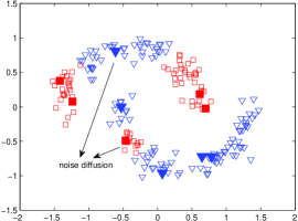
However, in the literature, the original motivation of developing these semi-supervised learning methods is to exploit both labeled and unlabeled data, but not to deal with the noise in the data. This means that they are not suitable for the challenging tasks (e.g. robust image analysis) where noisy initial labels are provided. To clearly show this disadvantage, we give a toy example in Fig. 1. We can observe that the negative effect of noisy labels is severely diffused by the traditional semi-supervised learning. Hence, our main motivation is just to develop a new semi-supervised learning method that can suppress the negative effect of noisy labels. Fortunately, in the following, the problem shown in Fig. 1 can be effectively handled by $L_{1}$-norm Laplacian regularization.

III-B $L_{1}$-Norm Laplacian Regularization

As reported in [17, 18], the sparsity induced by $L_{1}$-norm optimization can help to deal with the noise in the data to some extent. If we succeed in formulating Laplacian regularization as an $L_{1}$-norm term instead, we can convert the traditional semi-supervised learning to $L_{1}$-norm optimization and enable our new semi-supervised learning also to benefit from the nice property of sparsity (i.e. suppress the negative effect of noisy labels). Hence, in the following, we focus on $L_{1}$-norm formulation of Laplacian regularization.

Considering the important role that the normalized Laplacian matrix $\mathcal{L}$ plays in Laplacian regularization, we first give a symmetrical decomposition of $\mathcal{L}$. As a nonnegative definite matrix, $\mathcal{L}$ can be decomposed into

$$\mathcal{L}=V\Sigma V^{T},$$ (5)

where $V$ is an $n\times n$ orthonormal matrix with each column being an eigenvector of $\mathcal{L}$, and $\Sigma$ is an $n\times n$ diagonal matrix with its diagonal element $\Sigma_{ii}$ being an eigenvalue of $\mathcal{L}$ (sorted as $0\leq\Sigma_{11}\leq...\leq\Sigma_{nn}$). Furthermore, we represent $\mathcal{L}$ in the following symmetrical decomposition form:

$$\mathcal{L}=(\Sigma^{\frac{1}{2}}V^{T})^{T}\Sigma^{\frac{1}{2}}V^{T}=B^{T}B,$$ (6)

where $B=\Sigma^{\frac{1}{2}}V^{T}$. Since $B$ is computed with all the eigenvectors of $\mathcal{L}$, we can regard $B$ as being explicitly defined based upon the manifold structure of the data.

We further directly utilize $B$ to define a new $L_{1}$-norm smoothness measure, instead of the traditional smoothness measure used as Laplacian regularization for semi-supervised learning. In spectral graph theory, the smoothness of a vector $\mathbf{f}\in R^{n}$ is measured by $\Omega(\mathbf{f})=\mathbf{f}^{T}\mathcal{L}\mathbf{f}$, which is exactly the smoothness constraint in equation (3). Different from $\Omega(\mathbf{f})$, in this paper, the $L_{1}$-norm smoothness of a vector $\mathbf{f}\in R^{n}$ is measured by $\tilde{\Omega}(\mathbf{f})=||B\mathbf{f}||_{1}$. As for this new $L_{1}$-norm smoothness measure, we have the following proposition.

Proposition 1

(i) If $\tilde{\Omega}(\mathbf{f})\leq 1$, $\Omega(\mathbf{f})\leq\tilde{\Omega}(\mathbf{f})$; (ii) For an eigenvector $V_{.i}$ of $\mathcal{L}$, $\tilde{\Omega}(V.i)=\Sigma^{\frac{1}{2}}_{ii}$; (iii) If $\mathbf{f}=V\alpha=\sum_{i=1}^{n}\alpha_{i}V_{.i}$, $\tilde{\Omega}(\mathbf{f})=\sum_{i=1}^{n}|\alpha_{i}|\Sigma^{\frac{1}{2}}_{ii}$.

Proof: (i) If $\tilde{\Omega}(\mathbf{f})\leq 1$, $\Omega(\mathbf{f})=\mathbf{f}^{T}\mathcal{L}\mathbf{f}=\mathbf{f}^{T}B^{T}B\mathbf{f}=||B\mathbf{f}||_{2}^{2}=\sum_{i=1}^{n}(B_{i.}\mathbf{f})^{2}\leq(\sum_{i=1}^{n}|B_{i.}\mathbf{f}|)^{2}=||B\mathbf{f}||_{1}^{2}=(\tilde{\Omega}(\mathbf{f}))^{2}\leq\tilde{\Omega}(\mathbf{f})$, where $B_{i.}$ denotes the $i$-th row of $B$; (ii) $\tilde{\Omega}(V.i)=||BV_{.i}||_{1}=||\Sigma^{\frac{1}{2}}V^{T}V_{.i}||_{1}$. Since $V$ is orthonormal, we further have $\tilde{\Omega}(V.i)=||\Sigma^{\frac{1}{2}}[V_{.1}^{T}V_{.i},...,V_{.{i-1}}^{T}V_{.i},V_{.i}^{T}V_{.i},V_{.{i+1}}^{T}V_{.i},...,V_{.n}^{T}V_{.i}]^{T}||_{1}=||[0,...,0,\Sigma^{\frac{1}{2}}_{ii},0,...,0]^{T}||_{1}=\Sigma^{\frac{1}{2}}_{ii}$; (iii) $\tilde{\Omega}(\mathbf{f})=||B\mathbf{f}||_{1}=||(\Sigma^{\frac{1}{2}}V^{T})(V\alpha)||_{1}=||\sum_{i=1}^{n}\alpha_{i}\Sigma^{\frac{1}{2}}V^{T}V_{.i}||_{1}=||\sum_{i=1}^{n}\alpha_{i}[0,...,0,\Sigma^{\frac{1}{2}}_{ii},0,...,0]^{T}||_{1}=\sum_{i=1}^{n}|\alpha_{i}|\Sigma^{\frac{1}{2}}_{ii}$.

Proposition 1(i) shows that our $L_{1}$-norm smoothness can ensure the traditional smoothness if we succeed in reducing the former below 1. Proposition 1(ii) shows that eigenvectors with smaller eigenvalues are smoother in terms of our $L_{1}$-norm smoothness measure. Since any vector $\mathbf{f}\in R^{n}$ can be denoted as $\mathbf{f}=V\alpha=\sum_{i=1}^{n}\alpha_{i}V_{.i}$, we can conclude from Proposition 1(iii) that smooth vectors are linear combinations of the eigenvectors with small eigenvalues.

By replacing the traditional smoothness constraint (i.e. Laplacian regularization) in equation (3) with our $L_{1}$-norm version, we define a new objective function for graph-based semi-supervised learning as follows:

$$\tilde{Q}(\mathbf{f})=\frac{1}{2}||\mathbf{f}-\mathbf{y}||_{2}^{2}+\lambda||B\mathbf{f}||_{1}.$$ (7)

The first term of $\tilde{Q}(\mathbf{f})$ is the fitting constraint, while the second term is the $L_{1}$-norm smoothness constraint used as Laplacian regularization. Here, it should be noted that the fitting constraint is not formulated as an $L_{1}$-norm term. The reason is that most elements of $\mathbf{f}$ tend to zeros (i.e. sparsity) by $\min_{\mathbf{f}}||\mathbf{f}-\mathbf{y}||_{1}+\lambda||B\mathbf{f}||_{1}$ given that $\mathbf{y}$ has very few nonzero elements (i.e. very few initial labeled data are often provided for semi-supervised learning). In other words, the labels of data points are almost not propagated across the dataset, which completely conflicts with the original goal of semi-supervised learning. Hence, the fitting constraint of $\tilde{Q}(\mathbf{f})$ remains as an $L_{2}$-norm term. In the following, $L_{1}$-norm semi-supervised learning ($L_{1}$-SSL) refers to $\min_{\mathbf{f}}\tilde{Q}(\mathbf{f})$.

It is worth noting that our $L_{1}$-norm formulation of Laplacian regularization plays an important role in our explanation of $L_{1}$-norm semi-supervised learning in the framework of sparse coding. More concretely, according to Proposition 1(iii), our $L_{1}$-norm semi-supervised learning can be formulated as a linear reconstruction problem by setting $\mathbf{f}=V\alpha$. Furthermore, to solve this linear reconstruction problem efficiently, we can develop a fast sparse coding algorithm (see Section III-C) by working with only a small subset of eigenvectors (i.e. only partial columns of $V$ are used), which is especially suitable for robust image analysis tasks where the datasets are often large. Although there exist other $L_{1}$-norm generalizations [27, 28] of Laplacian regularization which approximately take the form of $\sum_{ij}w_{ij}|f_{i}-f_{i}|$, they are not explicitly defined based upon the eigenvectors of $\mathcal{L}$ and the strategy of dimension reduction is hard to be used for $\mathbf{f}$. Hence, the sparse coding algorithms developed in [27, 28] incur too large time cost.

Finally, we can similarly utilize $B$ to formulate the traditional Laplacian regularization as an $L_{2}$-norm term

$$\mathbf{f}^{T}\mathcal{L}\mathbf{f}=(B\mathbf{f})^{T}B\mathbf{f}=||B\mathbf{f}||_{2}^{2},$$ (8)

which is explicitly based upon the manifold structure of the data. Accordingly, the objective function $Q(\mathbf{f})$ of the traditional semi-supervised learning [9] can be redefined as the sum of two $L_{2}$-norm terms:

$$Q(\mathbf{f})=\frac{1}{2}||\mathbf{f}-\mathbf{y}||_{2}^{2}+\frac{\lambda}{2}||B\mathbf{f}||_{2}^{2}.$$ (9)

In the following, the traditional semi-supervised learning [9] is called as $L_{2}$-norm semi-supervised learning ($L_{2}$-SSL).

III-C Fast $L_{1}$-Norm Semi-Supervised Learning

As a convex optimization problem, our $L_{1}$-norm semi-supervised learning has a unique global solution $\mathbf{f}^{*}=\arg\min_{\mathbf{f}}\tilde{Q}(\mathbf{f})$. Let $\mathbf{x}=\mathbf{f}-\mathbf{y}$, $A=B$, and $\mathbf{b}=-B\mathbf{y}$. The original problem $\min_{\mathbf{f}}\tilde{Q}(\mathbf{f})$ for our $L_{1}$-norm semi-supervised learning is equivalently transformed into:

$$\min_{\mathbf{x}}\frac{1}{2}||\mathbf{x}||_{2}^{2}+\lambda||A\mathbf{x}-\mathbf{b}||_{1},$$ (10)

which is a new $L_{1}$-norm optimization problem. Similar to [35], a log-barrier algorithm can be readily developed for this $L_{1}$-norm optimization. However, the obtained log-barrier algorithm scales polynomially with the data size and then becomes impractical for image analysis tasks.

Fortunately, as we have mentioned in Section III-B, the dimension of our $L_{1}$-norm semi-supervised learning can be reduced dramatically by working only with a small subset of eigenvectors of $\mathcal{L}$. That is, similar to [36, 4], we significantly reduce the dimension of $\mathbf{f}$ by requiring it to take the form of $\mathbf{f}=V_{m}\alpha$ where $V_{m}$ is an $n\times m$ matrix whose columns are the $m$ eigenvectors with smallest eigenvalues (i.e. the first $m$ columns of $V$), which can simultaneously ensure that $\mathbf{f}$ is as smooth as possible in terms of our $L_{1}$-norm smoothness. According to equation (7), the objective function of our $L_{1}$-SSL can now be formulated as follows:

$$\tilde{Q}(\alpha) = \frac{1}{2}||(V_{m}\alpha)-\mathbf{y}||_{2}^{2}+\lambda||(\Sigma^{\frac{1}{2}}V^{T})(V_{m}\alpha)||_{1}$$ (11)

$$= \frac{1}{2}||V_{m}\alpha-\mathbf{y}||_{2}^{2}+\lambda||\sum_{i=1}^{m}\Sigma^{\frac{1}{2}}(V^{T}V_{.i})\alpha_{i}||_{1}$$

$$= \frac{1}{2}||V_{m}\alpha-\mathbf{y}||_{2}^{2}+\lambda\sum_{i=1}^{m}\Sigma^{\frac{1}{2}}_{ii}|\alpha_{i}|.$$

The first term of $\tilde{Q}(\alpha)$ denotes the linear reconstruction error, while the second term denotes the weighted $L_{1}$-norm sparsity regularization over the reconstruction coefficients. That is, our $L_{1}$-norm semi-supervised learning has successfully been transformed into a generalized sparse coding problem.

Algorithm 1 Fast $L_{1}$-SSL Algorithm

  Input: the initial label vector $\mathbf{y}$, the weight matrix $W$ of the $k$-NN graph, the number of smallest eigenvectors $m$, and the regularization parameter $\lambda$

  Output: the predicted labels by $\mathrm{sign}(\mathbf{f}^{*})$

  Step 1. Compute the normalized Laplacian matrix $\mathcal{L}=I-D^{-\frac{1}{2}}WD^{-\frac{1}{2}}$, where $D=\mathrm{diag}\{\sum_{j}W_{ij}\}$.

  Step 2. Find the $m$ smallest eigenvectors of $\mathcal{L}$ stored in $V_{m}$.

  Step 3. Solve the $L_{1}$-norm optimization problem $\alpha^{*}=\arg\min_{\alpha}\tilde{Q}(\alpha)$ using the modified FISTA.

  Step 4. Compute $\mathbf{f}^{*}=V_{m}\alpha^{*}$.

Figure 2: (a) The two-moons toy dataset with each class having one incorrectly (out of five) labeled data point initially. (b) The classification results on this toy dataset by our fast $L_{1}$-norm semi-supervised learning algorithm. Different from the traditional semi-supervised leaning, the negative effect of noisy labels can be completely suppressed by our new $L_{1}$-norm semi-supervised learning when noisy initial labels are provided.

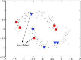
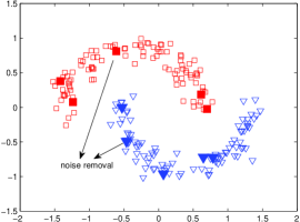
The formulation $\mathbf{f}=V_{m}\alpha$ used in equation (11) has two distinct advantages. Firstly, we can derive a linear reconstruction problem from the original semi-supervised learning problem, and correspondingly we can explain our $L_{1}$-norm semi-supervised learning in the framework of sparse coding. This also provides further insight into Laplacian regularization. In fact, the second term of $\tilde{Q}(\alpha)$ corresponds to both Laplacian regularization and sparsity regularization. By unifying these two types of regularization, we thus successfully obtain novel $L_{1}$-norm semi-supervised learning. Secondly, since $\tilde{Q}(\alpha)$ is minimized with respect to $\alpha\in R^{m}$ ($m\ll n$), we can readily develop fast sparse coding algorithms for our $L_{1}$-norm semi-supervised learning. That is, although many sparse coding algorithms scale polynomially with $m$, they have linear time complexity with respect to the data size $n$. More importantly, we have eliminated the need to compute the full matrix $B$ in equation (7), which is especially suitable for image analysis on large datasets. In fact, we only need to compute the $m$ smallest eigenvectors of $\mathcal{L}$. To speed up this step, we construct $k$-NN graphs for our $L_{1}$-norm semi-supervised learning. Given a $k$-NN graph ($k\ll n$), the time complexity of finding $m$ smallest eigenvectors of sparse $\mathcal{L}$ is $O(m^{3}+m^{2}n+kmn)$, which is scalable with respect to the data size $n$.

In theory, any fast sparse coding algorithm can be adopted to solve the $L_{1}$-norm optimization problem $\min_{\alpha}\tilde{Q}(\alpha)$. In this paper, we only consider the Fast Iterative Shrinkage-Thresholding Algorithm (FISTA) [19], since its implementation mainly involves lightweight operations such as vector operations and matrix-vector multiplications. To adjust the original FISTA for our $L_{1}$-norm semi-supervised learning, we only need to modify the soft-thresholding function as:

$$\mathrm{soft}(\alpha_{i},\frac{\lambda\Sigma^{\frac{1}{2}}_{ii}}{||V_{m}||_{s}^{2}})=\mathrm{sign}(\alpha_{i})\max\{|\alpha_{i}|-\frac{\lambda\Sigma^{\frac{1}{2}}_{ii}}{||V_{m}||_{s}^{2}},0\},$$ (12)

where $||V_{m}||_{s}$ represents the spectral norm of the matrix $V_{m}$. For large problems, it is often computationally expensive to directly compute the Lipschitz constant $||V_{m}||_{s}^{2}$. In practice, it can be efficiently estimated by a backtracking line-search strategy [19]. The complete algorithm for our fast $L_{1}$-norm semi-supervised learning is outlined in Algorithm 1. Since both Step 2 and Step 3 are scalable with respect to the data size $n$, our algorithm can be applied to large problems.

Figure 3: The quantitative comparison between $L_{2}$-SSL and $L_{1}$-SSL on the two-moons toy dataset given by Fig. 2. Here, $\mathbf{f}^{*}$ denotes the best solution found by $L_{2}$-SSL or $L_{1}$-SSL when $\lambda$ is set to the same value. The best solution found by our $L_{1}$-SSL is shown to be extremely smooth no matter which smoothness measure is considered, which is not true for $L_{2}$-SSL.

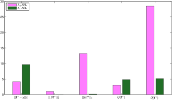
The classification results by our $L_{1}$-SSL algorithm on the two-moons toy dataset are shown in Fig. 2. We find that our algorithm can handle the problem (see Fig. 1) associated with the traditional $L_{2}$-SSL when noisy labels are provided initially. That is, our $L_{1}$-SSL algorithm can benefit from the nice property of sparsity induced by $L_{1}$-norm optimization and thus effectively suppress the negative effect of noisy labels. To give more convincing verification of such noise-robustness advantage, we further show a quantitative comparison between $L_{2}$-SSL and $L_{1}$-SSL in Fig. 3. The best solution $\mathbf{f}^{*}$ found by $L_{2}$-SSL or $L_{1}$-SSL is evaluated here by five quantitative measures such as the fitting error $||\mathbf{f}^{*}-\mathbf{y}||_{2}^{2}$, the traditional smoothness $||B\mathbf{f}^{*}||_{2}^{2}$, and the $L_{1}$-norm smoothness $||B\mathbf{f}^{*}||_{1}$.

We can clearly observe from Fig. 3 that the best solution $\mathbf{f}^{*}$ found by $L_{2}$-SSL is not smooth in terms of $||B\mathbf{f}^{*}||_{1}$, although smooth in terms of $||B\mathbf{f}^{*}||_{2}^{2}$. That is, considering the $L_{1}$-norm smoothness measure, we have indirectly shown that $L_{2}$-SSL can be severely misled by noisy labels (also consistent with Fig. 1). Here, it is worth noting that the less smooth a solution is, the poorer its generalization ability is (and thus more possible to be misled by the noise). On the contrary, the best solution $\mathbf{f}^{*}$ found by our $L_{1}$-SSL is shown to be extremely smooth no matter which smoothness measure is considered. Hence, by simultaneously controlling the fitting error below a low level, our $L_{1}$-SSL has successfully suppressed the negative effect of noisy labels (also consistent with Fig. 2).

IV Applications to Robust Image Analysis

Figure 4: The flowchart of sparse co-refinement of visual and textual BOW models by our $L_{1}$-norm semi-supervised learning only with linear kernel.

Considering the distinct advantage (i.e. noise robustness) of the proposed $L_{1}$-SSL algorithm, we apply it to two challenging tasks of robust image analysis: noise-robust semi-supervised image classification and noise reduction for both visual and textual BOW models. Although only tested in these two applications, the proposed $L_{1}$-SSL algorithm can be similarly extended to other image analysis tasks, since semi-supervised learning has been widely used in the literature.

IV-A Noise-Robust Semi-Supervised Image Classification

As the basis of many image analysis tasks such as image annotation and retrieval, semi-supervised image classification has been extensively studied in the literature [1, 2, 3, 4, 5]. In these applications, the manual labeling of training data is often tedious and expensive, while the access to unlabeled data is much easier. The original motivation of semi-supervised image classification is just to reduce the need for expensive labeled data by exploiting the large number of unlabeled data.

In this paper, we consider a more challenging problem, i.e., semi-supervised image classification with both correctly and incorrectly labeled data. In general, the occurrence of noisy labels may be due to the subjective manual labeling of training data. Fortunately, this challenging problem can be addressed to some extent by our $L_{1}$-SSL algorithm. As we have mentioned, our $L_{1}$-SSL algorithm can benefit from the nice property of sparsity induced by $L_{1}$-norm optimization and thus effectively suppress the negative effect of noisy labels. Since we focus on providing convincing verification of this noise-robustness advantage, we directly apply our $L_{1}$-SSL algorithm to semi-supervised image classification with noisy initial labels, without considering any preprocessing or postprocessing techniques. Hence, we only need to extend Algorithm 1 to multi-class problems commonly encountered in image analysis, which is elaborated in the following.

We first formulate a multi-class semi-supervised classification problem the same as [9]. Given a dataset $\mathcal{X}=\{x_{1},...,x_{l},x_{l+1},...,x_{n}\}$ and a label set $\{1,...,C\}$ ($C$ is number of classes), the first $l$ data points $x_{i}~{}(i\leq l)$ are labeled as: $y_{ij}=1$ if $x_{i}$ belongs to class $j$ ($1\leq j\leq C$) and $y_{ij}=0$ otherwise, while the remaining data points $x_{u}~{}(l+1\leq u\leq n)$ are unlabeled with $y_{uj}=0$. The goal of semi-supervised classification is to predict the labels of the unlabeled data points, i.e., to find a matrix $F=[f_{ij}]_{n\times C}$ corresponding to a classification on the dataset $\mathcal{X}$ by labeling each data point $x_{i}$ with a label $\arg\max_{1\leq j\leq C}f_{ij}$. Let $Y=[y_{ij}]_{n\times C}$, and we can readily observe that $Y$ is exactly consistent with the initial labels according to the decision rule. When noisy initial labels are provided for semi-supervised classification, some entries of $Y$ may be inconsistent with the ground truth.

Based on the above preliminary notations, we further formulate our multi-class $L_{1}$-SSL problem as:

$$\min_{F}\tilde{Q}(F)=\min_{F}\frac{1}{2}||F-Y||_{F}^{2}+\lambda||BF||_{1},$$ (13)

which can be decomposed into $C$ independent subproblems:

$$\min_{F_{.j}}\tilde{Q}(F_{.j})=\min_{F_{.j}}\frac{1}{2}||F_{.j}-Y_{.j}||_{2}^{2}+\lambda||BF_{.j}||_{1},$$ (14)

where $F_{.j}$ and $Y_{.j}$ denote the $j$-th column of $F$ and $Y$, respectively. Since each subproblem $\min_{F_{.j}}\tilde{Q}(F_{.j})$ can be regarded as a two-class problem, we can readily solve it by Algorithm 1. Let $F_{.j}^{*}=\arg\min_{F_{.j}}\tilde{Q}(F_{.j})$, and we can classify $x_{i}$ into class $\arg\max_{1\leq j\leq C}f_{ij}^{*}$.

IV-B Sparse Co-Refinement of Visual and Textual BOW Models

We further pay attention to visual and textual BOW refinement to obtain robust image representation, which is different from semi-supervised image classification as a high-level semantic analysis task. Although both visual and textual BOW models have been shown to achieve impressive results, each BOW model has its own drawbacks. Firstly, since the visual BOW model generally creates a visual vocabulary by clustering on the local descriptors extracted from images, the visual vocabulary may be far from accurate due to the inherent limitation of clustering and thus the labels of local descriptors may be rather noisy. This means that visual BOW refinement is crucial for the success of BOW-based image analysis tasks. Secondly, instead of the expensive manual labeling of images, the textual BOW model for image representation is commonly based upon the image tags contributed by the community (e.g. Flickr) or automatically derived from the associated text (e.g. Web page). Because the tags of an image obtained in these ways may be incorrect and incomplete, the problem of textual BOW refinement becomes rather challenging.

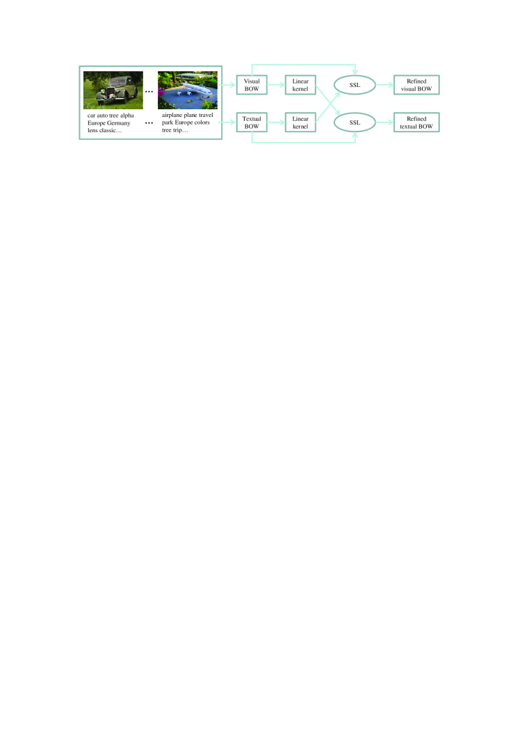
To address the above problems, we propose a novel framework for sparse co-refinement of visual and textual BOW models by our $L_{1}$-SSL algorithm, as shown in Fig. 4. Our basic idea is to formulate BOW refinement as a multi-class semi-supervised learning (SSL) problem by regarding each word of the BOW model as a “class” so that our noise-robust $L_{1}$-SSL algorithm can be applied to noise reduction for both visual and textual BOW models. Since textual BOW refinement is actually a dual problem of visual BOW refinement, we focus on visual BOW refinement in the following.

Let $Y\in R^{n\times M}$ be the visual BOW representation and $B\in R^{n\times n}$ be computed based on the textual BOW representation, where $n$ is the number of images and $M$ is the number of visual words. To compute $B$ according to equation (6), we only consider a linear kernel matrix (used as the weight matrix $W$) defined with the textual BOW representation. The visual BOW refinement problem can be formulated as:

$$\min_{F}\frac{1}{2}||F-Y||_{F}^{2}+\lambda||BF||_{1}+\gamma||F-Y||_{1},$$ (15)

where $\lambda$ and $\gamma$ denote two regularization parameters. As compared to the $L_{1}$-SSL problem given by equation (13), the only difference is that another $L_{1}$-norm regularization term (i.e. $||F-Y||_{1}$) is considered for visual BOW refinement.

As we have mentioned in Section III-B, we do not formulate the fitting constraint as an $L_{1}$-norm term for our $L_{1}$-SSL because the predicted labels will be too sparse when very few labeled data are provided initially. As a truth, the sparsity of predicted labels completely conflicts with the original goal of semi-supervised learning. However, the case is quite different for visual BOW refinement, i.e., a large number of initial labeled data are provided since each visual word can be assigned to many images. Hence, the predicted labels may not be sparse even if the $L_{1}$-norm fitting constraint is used for semi-supervised learning. Here, our main motivation of considering $||F-Y||_{1}$ is to induce the fitting error sparsity and thus impose direct noise reduction on $Y$.

Although we can find a unique global solution for the visual BOW refinement problem by convex optimization, it is not easy to develop an efficient algorithm for this convex optimization. Fortunately, we can approximately solve it in two $L_{1}$-norm optimization steps: (1) $Y^{*}=\arg\min_{F}\frac{1}{2}||F-Y||_{F}^{2}+\lambda||BF||_{1}$; (2) $F^{*}=\arg\min_{F}\frac{1}{2}||F-Y^{*}||_{F}^{2}+\gamma||F-Y||_{1}$. The first optimization subproblem can be efficiently solved by our $L_{1}$-SSL algorithm, while the second subproblem has an explicit solution based on the soft-thresholding function:

$$F^{*}=\mathrm{soft}(Y^{*}-Y,\gamma)+Y,$$ (16)

where the definition of $\mathrm{soft}(\cdot,\cdot)$ can be found in equation (12). Considering the scalability of our $L_{1}$-SSL algorithm with respect to the data size, the visual BOW refinement problem can be solved in a linear time cost.

As a dual problem, the textual BOW refinement can be formulated in the same form of equation (15) by computing $B$ using the visual BOW representation instead. In summary, we have successfully solve the challenging problem of sparse co-refinement of visual and textual BOW models based on our $L_{1}$-SSL algorithm. To our best knowledge, we have made the first attempt to obtain robust image representation by sparse co-refinement of visual and textual BOW models, which is extremely important for the success of robust image analysis on community-contributed image collections (e.g. Flickr). However, in the literature, most previous methods can not deal with visual and textual BOW refinement simultaneously. For example, various supervised [29, 30] and unsupervised [31, 32] methods have been developed specially for visual vocabulary optimization, while in [33, 34, 5] only tag refinement is considered for robust image analysis.

It is worth noting that the supervisory information is usually expensive to obtain for visual vocabulary optimization in [29, 30], while the access to the image tags used for our visual BOW refinement is much easier (although noisy). Moreover, the use of image tags also distinguishes our visual BOW refinement method from the unsupervised methods [31, 32] without considering any high-level semantic information for visual vocabulary optimization. As compared to the closely related work [5] on tag refinement that only adopts the traditional Laplacian regularization for semi-supervised learning, this paper has formulated new $L_{1}$-norm Laplacian regularization which has a wide and important use in the literature.

V Experimental Results

In this section, our $L_{1}$-SSL algorithm is tested in two applications: noise-robust image classification and co-refinement of visual and textual BOW models. In particular, to show the descriptive power of the refined BOW models, we apply them to supervised classification with SVM, different from semi-supervised classification in the first application.

V-A Noise-Robust Image Classification

We evaluate our $L_{1}$-SSL algorithm for noise-robust image classification on the four image datasets listed in Table I. We first describe the experimental setup and then compare our $L_{1}$-SSL algorithm with other closely related methods.

V-A1 Experimental Setup

TABLE I: Details of the four image datasets including two handwritten digit datasets and two natural image datasets.

Datasets	MNIST	USPS	Corel	Scene
#samples	10,000	9,298	2,000	2,688
#features	784	256	400	400
#classes	10	10	20	8

Our $L_{1}$-norm semi-supervised learning ($L_{1}$-SSL) is compared to four other representative methods: (1) the traditional $L_{2}$-norm semi-supervised learning ($L_{2}$-SSL) [9], (2) Lasso-based $L_{1}$-norm semi-supervised learning (Lasso-SSL) [24], (3) linear neighborhood propagation (LNP) [12], and (4) support vector machine (SVM). To make an extensive comparison, we conduct two groups of experiments: semi-supervised classification with a varying number of clean initial labeled images, and noise-robust classification with a varying percentage of noisy initial labeled images. The test accuracies on the unlabeled images are averaged over 25 independent runs and used for performance evaluation.

Figure 5: Illustration of the effect of different parameters on our $L_{1}$-SSL algorithm with 50 clean initial labeled images for the two handwritten digit datasets. First Row: MNIST. Second Row: USPS.

Figure 6: The classification results (%) on the four image datasets by different algorithms when a varying number of clean labeled images are initially provided. The error bar indicates the 95% confidence interval.

We adopt two different approaches to kernel matrix computation. Firstly, for the two handwritten digit datasets (i.e. MNIST and USPS), we compute the Gaussian kernel matrix according to equation (1) with fixed $\sigma=1$. Secondly, for the two natural image datasets (i.e. Scene and Corel), we compute the spatial Markov kernel matrix [37] based on 400 visual words (i.e. 400 features), just the same as [38]. The kernel matrix can be directly used for SVM, while for semi-supervised learning we can regard it as the weight matrix so that a $k$-NN graph can be constructed. The $k$-NN graph is further refined for LNP by quadratic programming [12].

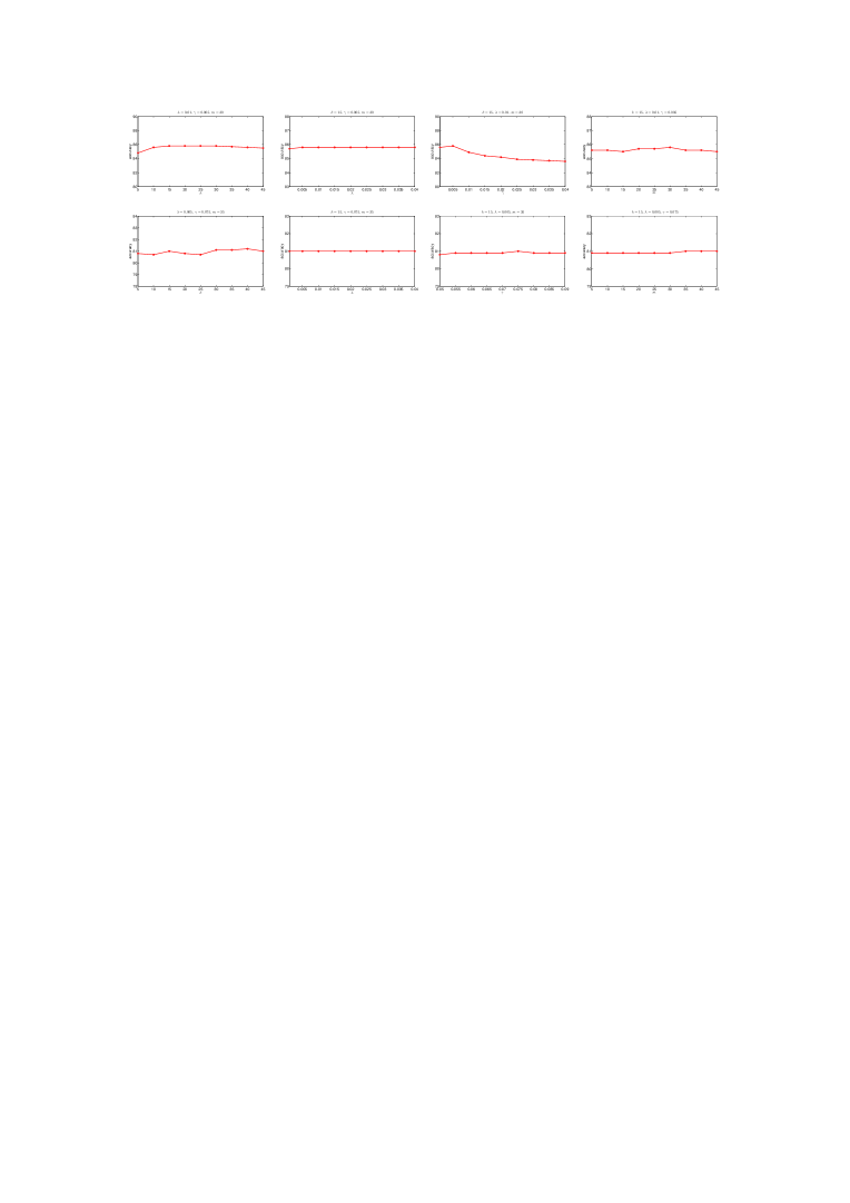
We empirically select $k=4$, $\lambda=0.01$ and $m=20$ for our $L_{1}$-SSL algorithm on the two handwritten digit datasets. Here, it should be noted that both $k$ and $m$ are determined by the consideration of the tradeoff between running efficiency and classification performance, i.e., we always prefer smaller $k$ and $m$ for our $L_{1}$-SSL algorithm when there only exists little performance degradation. More importantly, as shown in Fig. 5, our $L_{1}$-SSL algorithm is generally not much sensitive to these parameters. The same strategy of parameter selection is adopted for our $L_{1}$-SSL algorithm on the two natural image datasets, while the parameters of other related algorithms for comparison are also set their respective optimal values.

V-A2 Classification Results

Figure 7: The classification results (%) on the four image datasets by different algorithms when a varying percentage of noisy labels are provided (among totally $5\times$#classes initial labeled images). The error bar indicates the 95% confidence interval.

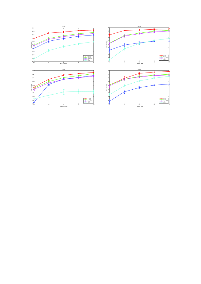
Although our original motivation is to apply our $L_{1}$-SSL to noise-robust classification, we first compare the five different methods in the less challenging task of semi-supervised classification with clean initial labeled images to verify their effectiveness in dealing with the scarcity of labeled images. The comparison results are shown in Fig. 6, where the 95% confidence intervals are also provided. In general, we can observe that our $L_{1}$-SSL consistently performs the best among all the five methods. The reason may be that our $L_{1}$-SSL can benefit form the sparsity induced by our $L_{1}$-norm Laplacian regularization and thus suppress the negative effect of the complicated manifold structure hidden among images on semi-supervise classification. It should be noted that the four image datasets have much more complicated structures than the two-moons toy dataset shown in Fig. 1, which are really challenging to deal with for the other four methods including $L_{2}$-SSL. Interestingly, although an $L_{1}$-norm semi-supervised learning strategy is also adopted, Lasso-SSL [24] ignores the important Laplacian regularization and thus generally performs the worst among the four SSL methods.

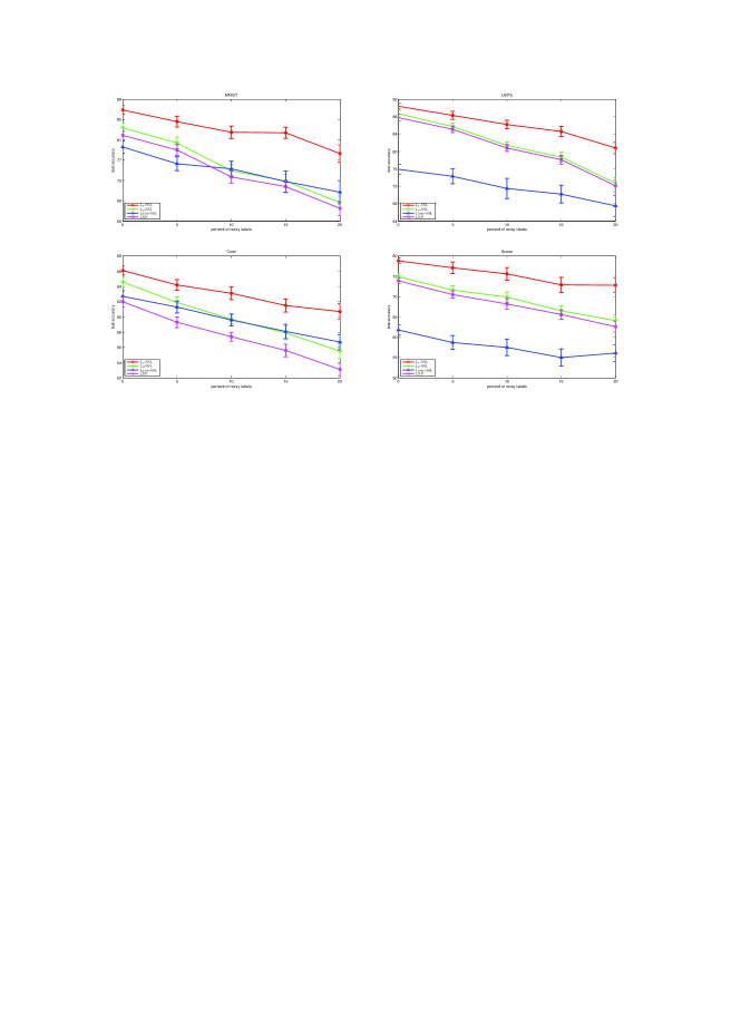
We make further comparison in the challenging task of noise-robust classification with noisy initial labeled images. Since the four SSL methods have been shown to generally outperform SVM (see Fig. 6), we focus on verifying the effectiveness of noise reduction by semi-supervised learning in the following. The comparison results on noise-robust classification are shown in Fig. 7. We find that our $L_{1}$-SSL consistently achieves significant gains over the other SSL methods, especially when more noisy labels are provided initially. That is, our $L_{1}$-norm Laplacian regularization indeed can help to find a smooth and also sparse solution for semi-supervised learning and thus effectively suppress the negative effect of noisy labels. More importantly, although all the four methods suffer from more performance degradation when the percentage of noisy labels grows, the performance of $L_{1}$-SSL and Lasso-SSL degrades the slowest due to that they both utilize sparse coding for semi-supervised learning.

Besides the above advantages, our $L_{1}$-SSL has another advantage in terms of running efficiency, i.e., it runs the fastest among the four SSL algorithms. For example, the time taken by $L_{1}$-SSL, $L_{2}$-SSL, Lasso-SSL, and LNP on the MNIST dataset with 50 clean labeled images is 39, 57, 433, and 132 seconds, respectively. We run all the algorithms (Matlab code) on a server with 3GHz CPU and 31.9GB RAM.

Figure 8: The twofold cross-validation results by our $L_{1}$-SSL algorithm on the training set of the Flickr image dataset. First Row: visual BOW refined with textual BOW. Second Row: textual BOW refined with visual BOW.

V-B Visual and Textual BOW Refinement

In this subsection, our $L_{1}$-SSL algorithm is applied to sparse co-refinement of visual and textual BOW models. To verify the descriptive power of the refined BOW models, we focus on evaluating them in SVM-based image classification. Here, it should be noted that the refined BOW models can also be readily extended to many other image analysis tasks such as content-based and text-based image retrieval. Moreover, although the visual and textual BOW refinement problems can be solved by any SSL method (see Fig. 4), we only make comparison between our $L_{1}$-SSL and $L_{2}$-SSL, since they have both been shown to generally outperform the other SSL methods in the above experiments.

V-B1 Experimental Setup

We conduct a group of experiments on a Flickr benchmark dataset [39], which consists of totally 8,564 images crawled from the photo sharing website Flickr. This image dataset is organized into eleven categories: airplane, auto, dog, turtle, elephant, NBA, laptop, piano, farm, cityscape and library. The high-level category labels of images can be used for SVM-based image classification. In the following experiments, we split this dataset into a training set of 4,282 images and a test set of the same size.

To obtain the visual BOW representation for the Flickr dataset, we extract the SIFT descriptors of $16\times 16$ pixel blocks computed over a regular grid with spacing of 8 pixels. We then perform $k$-means clustering on the extracted descriptors to form a vocabulary of 2,000 visual words. Here, we aim to make the visual BOW representation more noisy by considering a relatively larger visual vocabulary. Moreover, we generate the textual BOW representation based on the user-provided textual tags. As a preprocessing step, we remove the stop words and check the remaining tags against the WordNet to remove the tags that do not exist. The final textual vocabulary only contains the most frequent 1,000 words.

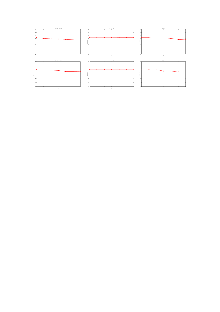
From these two BOW representations, we only derive linear kernels for our $L_{1}$-SSL algorithm in the tasks of visual and textual BOW refinement. Based on the obtained kernel matrices, we can further construct $k$-NN graphs for semi-supervised learning. The linear kernels are also used for the subsequent SVM classification. According to the twofold cross-validation results on the training set as shown in Fig. 8, we set the parameters of our $L_{1}$-SSL algorithm to their respective optimal values listed in Table II. Just as what we have done in noise-robust image classification, we still determine both $k$ and $m$ by the consideration of the tradeoff between running efficiency and classification performance. More importantly, we can clearly observe from Fig. 8 that our $L_{1}$-SSL algorithm is not much sensitive to these parameters in most cases.

V-B2 Refinement Results

TABLE II: The parameters selected by cross-validation for our $L_{1}$-SSL algorithm in both visual and textual BOW refinement.

Parameters	$k$	$\lambda$	$\gamma$	$m$
Visual BOW	15	0.010	0.005	30
Textual BOW	15	0.005	0.075	35

TABLE III: The classification results (%) on the Flickr image dataset using different BOW models. Both $L_{2}$-SSL and $L_{1}$-SSL can be used for co-refinement of visual and textual BOW models.

Methods	Original	[5]	$L_{2}$-SSL	$L_{1}$-SSL
Visual BOW	60.1	78.2	84.3	87.4
Textual BOW	77.8	81.4	81.5	83.2

To show the effectiveness of visual and textual BOW refinement, we compare the refined BOW models by our $L_{1}$-SSL to: (1) the original BOW models, (2) the refined BOW models by the SSL method proposed in [5], and (3) the refined BOW models by $L_{2}$-SSL. The comparison results are list in Table III. The immediate observation is that the refined BOW models by our $L_{1}$-SSL lead to obvious gains over the original BOW models, especially when the visual BOW model is refined with the textual BOW model (i.e. 27.3% gain). This means that our $L_{1}$-SSL for visual and textual BOW refinement indeed can benefit from the sparsity induced by $L_{1}$-norm optimization and thus effectively suppress the noise in both visual and textual BOW models.

Moreover, we can clearly observe from Table III that $L_{2}$-SSL also achieves promising results in visual and textual BOW refinement, although it is not originally developed for noise reduction. The reason may be that the visual (or textual) words associated with each image in the Flickr dataset are not only noisy but also incomplete due to inaccurate clustering (or subjective and limited manual labeling), while the issue of incomplete words can be effectively handled by word propagation based on $L_{2}$-SSL. Here, it is worth noting that, different from the traditional $L_{2}$-SSL, our $L_{1}$-SSL is suitable for both word propagation and noise reduction. Hence, as shown in Table III, our $L_{1}$-SSL performs better than $L_{2}$-SSL in both visual and textual BOW refinement.

As for the SSL method [5], we find that it works nearly as well as $L_{2}$-SSL in textual BOW refinement, but leads to much worse results in visual BOW refinement. Its promising performance in textual BOW refinement may be due to that it can perform both noise reduction and word propagation by imposing the fitting error sparsity on SSL. However, the case is different for visual BOW refinement, i.e., the issue of incomplete words may be more severe for wrong label permutation along with inaccurate clustering. As compared to $L_{2}$-SSL [9] (one of the most outstanding SSL methods), the SSL method [5] has a poorer performance of visual word propagation and thus suffers from obvious degradation.

VI Conclusions

We have proposed a novel $L_{1}$-norm semi-supervised learning method in this paper. Different from the traditional graph-based SSL that defines Laplacian regularization by a quadratic function, we have successfully reformulated Laplacian regularization as an $L_{1}$-norm term. More importantly, we find that this new formulation is explicitly based upon the manifold structure of the data. Due to the resulting $L_{1}$-norm optimization, our new $L_{1}$-SSL can benefit from the nice property of sparsity and thus effectively suppress the negative effect of noisy labels. Extensive results have shown the promising performance of our $L_{1}$-SSL in two challenging tasks of robust image analysis. In the future work, considering the wide use of Laplacian regularization, we will apply our new $L_{1}$-norm Laplacian regularization to many other challenging problems. Moreover, the refined visual and textual BOW models by our $L_{1}$-SSL will be evaluated in other image analysis tasks such as content-based and text-based image retrieval.

Zhiwu Lu received the M.Sc. degree in applied mathematics from Peking University, Beijing, China in 2005, and the Ph.D. degree in computer science from City University of Hong Kong in 2011. Since March 2011, he has become an assistant professor with the Institute of Computer Science and Technology, Peking University. He has published over 30 papers in refereed international journals and conference proceedings including TIP, TSMC-B, TMM, AAAI, ICCV, CVPR, ECCV, and ACM-MM. His research interests lie in machine learning, pattern recognition, computer vision, and multimedia information retrieval.

Yuxin Peng is the professor and director of Multimedia Information Processing Lab (MIPL) in the Institute of Computer Science and Technology (ICST), Peking University. He received his Ph.D. degree in computer application from School of Electronics Engineering and Computer Science (EECS), Peking University, in Jul. 2003. After that, he worked as an assistant professor in ICST, Peking University. From Aug. 2003 to Nov. 2004, he was a visiting scholar with the Department of Computer Science, City University of Hong Kong. He was promoted to associate professor in Peking University in Aug. 2005. In Aug. 2010, he was promoted to professor in Peking University. He has published over 50 papers in refereed international journals and conference proceedings including TCSVT, TIP, ACM-MM, ICCV, CVPR and AAAI. In 2009, he led his team to participate in TRECVID. In six tasks of the high-level feature extraction (HLFE) and search, his team won the first places in fours tasks and the second places in the left two tasks. Besides, he has obtained 12 patents. His current research interests include multimedia information retrieval, image processing, computer vision, and pattern recognition.

References

- [1] D. Xu and S. Yan, “Semi-supervised bilinear subspace learning,” IEEE Trans. Image Processing, vol. 18, no. 7, pp. 1671–1676, 2009.
- [2] M. Guillaumin, J. Verbeek, and C. Schmid, “Multimodal semi-supervised learning for image classification,” in Proc. CVPR, 2010, pp. 902–909.
- [3] Z. Lu and H. Ip, “Combining context, consistency, and diversity cues for interactive image categorization,” IEEE Trans. Multimedia, vol. 12, no. 3, pp. 194–203, 2010.
- [4] R. Fergus, Y. Weiss, and A. Torralba, “Semi-supervised learning in gigantic image collections,” in Advances in Neural Information Processing Systems 22, 2010, pp. 522–530.
- [5] J. Tang, S. Yan, R. Hong, G.-J. Qi, and T.-S. Chua, “Inferring semantic concepts from community-contributed images and noisy tags,” in Proc. ACM Multimedia, 2009, pp. 223–232.
- [6] J. Liu, M. Li, Q. Liu, H. Lu, and S. Ma, “Image annotation via graph learning,” Pattern Recognition, vol. 42, no. 2, pp. 218–228, 2009.
- [7] A. Blum and T. Mitchell, “Combining labeled and unlabeled data with co-training,” in Proc. COLT, 1998.
- [8] X. Zhu, Z. Ghahramani, and J. Lafferty, “Semi-supervised learning using Gaussian fields and harmonic functions,” in Proc. ICML, 2003, pp. 912–919.
- [9] D. Zhou, O. Bousquet, T. Lal, J. Weston, and B. Schölkopf, “Learning with local and global consistency,” in Advances in Neural Information Processing Systems 16, 2004, pp. 321–328.
- [10] A. Corduneanu and T. Jaakkola, “Distributed information regularization on graphs,” in Advances in Neural Information Processing Systems 17, 2005, pp. 297–304.
- [11] R. Ando and T. Zhang, “Learning on graph with Laplacian regularization,” in Advances in Neural Information Processing Systems 19, 2007, pp. 25–32.
- [12] F. Wang and C. Zhang, “Label propagation through linear neighborhoods,” IEEE Trans. Knowledge and Data Engineering, vol. 20, no. 1, pp. 55–67, 2008.
- [13] S. Yan and H. Wang, “Semi-supervised learning by sparse representation,” in Proc. SIAM International Conference on Data Mining (SDM), 2009, pp. 792–801.
- [14] B. Cheng, J. Yang, S. Yan, Y. Fu, and T. Huang, “Learning with -graph for image analysis,” IEEE Trans. Image Processing, vol. 19, no. 4, pp. 858–866, 2010.
- [15] W. Liu, J. He, and S.-F. Chang, “Large graph construction for scalable semi-supervised learning,” in Proc. ICML, 2010, pp. 679–686.
- [16] B. Nadler, N. Srebro, and X. Zhou, “Statistical analysis of semi-supervised learning: The limit of infinite unlabelled data,” in Advances in Neural Information Processing Systems 22, 2010, pp. 1330–1338.
- [17] D. Donoho, “For most large underdetermined systems of linear equations the minimal -norm solution is also the sparsest solution,” Communications on Pure and Applied Mathematics, vol. 59, no. 7, pp. 797–829, 2004.
- [18] J. Wright, A. Yang, A. Ganesh, S. Sastry, and Y. Ma, “Robust face recognition via sparse representation,” IEEE Trans. Pattern Analysis and Machine Intelligence, vol. 31, no. 2, pp. 210–227, 2009.
- [19] A. Beck and M. Teboulle, “A fast iterative shrinkage-thresholding algorithm for linear inverse problems,” SIAM Journal on Imaging Sciences, vol. 2, no. 1, pp. 183–202, 2009.
- [20] M. Osborne, B. Presnell, and B. Turlach, “A new approach to variable selection in least squares problems,” IMA Journal of Numerical Analysis, vol. 20, no. 3, pp. 389–403, 2000.
- [21] M. Figueiredo, R. Nowak, and S. Wright, “Gradient projection for sparse reconstruction: Application to compressed sensing and other inverse problems,” IEEE Journal of Selected Topics in Signal Processing, vol. 1, no. 4, pp. 586–597, 2007.
- [22] H. Lee, A. Battle, R. Raina, and A. Ng, “Efficient sparse coding algorithms,” in Advances in Neural Information Processing Systems 19, 2007, pp. 801–808.
- [23] W. Dai and O. Milenkovic, “Subspace pursuit for compressive sensing signal reconstruction,” IEEE Trans. Information Theory, vol. 55, no. 5, pp. 2230–2249, 2009.
- [24] K. Sinha and M. Belkin, “Semi-supervised learning using sparse eigenfunction bases,” in Advances in Neural Information Processing Systems 22, 2010, pp. 1687–1695.
- [25] R. Tibshirani, “Regression shrinkage and selection via the Lasso,” Journal of the Royal Statistical Society, Series B, vol. 58, no. 1, pp. 267–288, 1996.
- [26] S. Gao, I. Tsang, L.-T. Chia, and P. Zhao, “Local features are not lonely - Laplacian sparse coding for image classification,” in Proc. CVPR, 2010, pp. 3555–3561.
- [27] X. Chen, Q. Lin, S. Kim, J. Carbonell, and E. Xing, “An efficient proximal gradient method for general structured sparse learning,” 2010. [Online]. Available: http://arxiv.org/abs/1005.4717
- [28] S. Petry, C. Flexeder, and G. Tutz, “Pairwise fused Lasso,” 2011. [Online]. Available: http://epub.ub.uni-muenchen.de/12164/
- [29] L. Yang, R. Jin, R. Sukthankar, and F. Jurie, “Unifying dis-criminative visual codebook generation with classifier training for object category reorganization,” in Proc. CVPR, 2008.
- [30] P. Mallapragada, R. Jin, and A. Jain, “Online visual vocabulary pruning using pairwise constraints,” in Proc. CVPR, 2010, pp. 3073–3080.
- [31] R. Ji, X. Xie, H. Yao, and W.-Y. Ma, “Vocabulary hierarchy optimization for effective and transferable retrieval,” in Proc. CVPR, 2009, pp. 1161–1168.
- [32] Z. Lu, Y. Peng, and H. Ip, “Spectral learning of latent semantics for action recognition,” in Proc. ICCV, 2011.
- [33] S. Lee, W. Neve, and Y. Ro, “Tag refinement in an image folksonomy using visual similarity and tag co-occurrence statistics,” Signal Processing: Image Communication, vol. 25, no. 10, pp. 761–773, 2010.
- [34] G. Zhu, S. Yan, and Y. Ma, “Image tag refinement towards low-rank, content-tag prior and error sparsity,” in Proc. ACM Multimedia, 2010, pp. 461–470.
- [35] S. Boyd and L. Vandenberghe, Eds., Convex Optimization. New York: Cambridge University Press, 2004.
- [36] O. Chapelle, B. Scholköpf, and A. Zien, Eds., Semi-Supervised Learning. MIT Press, 2006.
- [37] Z. Lu and H. Ip, “Spatial Markov kernels for image categorization and annotation,” IEEE Trans. Systems, Man, and Cybernetics - Part B, vol. 41, no. 4, pp. 976–989, 2011.
- [38] ——, “Constrained spectral clustering via exhaustive and efficient constraint propagation,” in Proc. ECCV, vol. 6, 2010, pp. 1–14.
- [39] Z. Fu, H. Ip, H. Lu, and Z. Lu, “Multi-modal constraint propagation for heterogeneous image clustering,” in Proc. ACM Multimedia, 2011.
![[Uncaptioned image]](/html/1110.3109/assets/x11.png) |