Spectra of Harmonium in a magnetic field using an initial value representation of the semiclassical propagator

Abstract

For two Coulombically interacting electrons in a quantum dot with harmonic confinement and a constant magnetic field, we show that time-dependent semiclassical calculations using the Herman-Kluk initial value representation of the propagator lead to eigenvalues of the same accuracy as WKB calculations with Langer correction. The latter are restricted to integrable systems, however, whereas the time-dependent initial value approach allows for applications to high-dimensional, possibly chaotic dynamics and is extendable to arbitrary shapes of the potential.

1 Introduction

The problem of two interacting electrons in atoms, ions and molecules is of fundamental importance in quantum mechanics, the understanding of the Helium atom being one of the prime successes of the “new quantum mechanics” [1]. If the Coulombic interaction between electrons and nucleus is replaced by a harmonic confining potential, the system is referred to as Harmonium, quantum dot Helium or Hooke’s law atom. After early work without additional magnetic field [2], this problem, with and without a magnetic field, has again come in the focus of interest in the past 20 years mainly for two different reasons:

Firstly it is of principal interest to find (exact) analytic solutions for a problem with genuine Coulomb interaction. That such exact solutions do exist has been shown for two electrons in a harmonic confinement in 3 dimensions, without an additional magnetic field [2, 3], and in 2 dimensions with a magnetic field by Verçin [4] and Taut [5]. The existence of closed solutions for specific ratios of the Coulomb interaction and the harmonic potential is related to an accidental (hidden) symmetry visible after mapping the Coulomb interaction to a four dimensional harmonic oscillator potential [6]. Furthermore, in 2 dimensions and using perturbation theory for the Coulomb interaction, analytic solutions have been given in [7]. The analytic solutions can be put to good use in the testing of density functionals and other methods for many-body systems [8, 9, 10]. Secondly, due to recent progress in nanofabrication, few electron quantum dots have come into the limelight as they may provide a realization of a quantum bit [11].

Due to the fact that exact analytic solutions of the Schödinger equation are limited to an infinite set of discrete oscillator frequencies [3, 5], also approximate analytic solutions have been sought for. Apart from the perturbation theoretic ones in 2d, mentioned above, also semiclassical approaches have been taken which rely on the Wentzel-Kramers-Brillouin (WKB) [12], respectively the Einstein-Brillouin-Keller (EBK) quantization rules [13]. Most notably, in 2d and with an additional magnetic field this has been done analytically by Klama and Mishchenko [14]. It turned out that the problem of two electrons in 2d, although one of 4 degrees of freedom (DOF), is highly separable and therefore in the end only a 1 DOF WKB approach is needed, which describes the spectrum with a high accuracy. In another semiclassical analysis of the harmonium problem, including a magnetic field, dimensional effects have been discussed by Nazmitdinov and collaborators [15].

Whereas in WKB energy information is directly available, using the semiclassical initial value representation (IVR) of the quantum mechanical propagator of Herman and Kluk (HK) [16, 17, 18] spectra can be gained by Fourier transformation of a time series, usually an auto-correlation function [19]. In [20] it has been shown that accurate spectra for collinear Helium can be obtained in this way. Furthermore, semiclassical work on one electron systems in external laser fields gives the explanation for the plateau formation in high harmonic spectra [21].

In this paper we will show that the time-dependent semiclassical approach, complementary to the energy-domain WKB method, is also capable of reproducing high quality spectra for 2d Harmonium in a homogeneous magnetic field. Thus adding to the knowledge of semiclassics for interacting many particle dynamics is not a mere exercise due to the fact that the time-dependent approach is not principally restricted in dimensionality nor to the case of a circular quantum dot and also additional time-dependent potentials may be treated in a similar fashion without much more effort. In Sec. 2, the Hamiltonian is briefly introduced, whereas in Sec. 3 we review the semiclassical IVR of Herman and Kluk based on frozen Gaussian wavepackets. The new results we gained are compared with full quantum as well as with (Langer-corrected) WKB results in Sec. 4 and we give conclusions and an outlook in Sec. 5.

2 The Hamiltonian

The Hamiltonian for the problem of two charged particles (charge $q$) in a 2d circular quantum dot (dielectric constant $\epsilon$) with a confinement frequency of $\omega_{0}$ inside a magnetic field, derived from a vector potential $\mbox{\bf A}(\mbox{\bf r}_{i})$ is given by

$$H=\sum_{i=1}^{2}\left(\frac{(\mbox{\bf p}_{i}-q\mbox{\bf A}(\mbox{\bf r}_{i}))^{2}}{2m^{\ast}}+\frac{1}{2}m^{\ast}\omega_{0}^{2}\mbox{\bf r}_{i}^{2}\right)+\frac{\kappa}{|\mbox{\bf r}_{1}-\mbox{\bf r}_{2}|}.$$ (1)

Here $\kappa=q^{2}/(4\pi\epsilon\epsilon_{0})$ and for two electrons $m^{\ast}$ is the (effective) mass and the charge is $q=-e$. We are not explicitly taking into account electron spin, thereby neglecting the Zeeman energy of the spins in the magnetic field, see also [15]. In addition, as will be seen and commented on below (see Section 4.2), for the propagation in time, we will consider an unsymmetrized position-dependent part of the quantum mechanical wavefunction.

To make progress, center of mass (cm) and relative coordinates are introduced, according to

$$\mbox{\bf R}=\frac{1}{2}(\mbox{\bf r}_{1}+\mbox{\bf r}_{2})\qquad\mbox{\bf P}=(\mbox{\bf p}_{1}+\mbox{\bf p}_{2}),$$ (2)

respectively

$$\mbox{\bf r}=\mbox{\bf r}_{1}-\mbox{\bf r}_{2}\qquad\mbox{\bf p}=\frac{1}{2}(\mbox{\bf p}_{1}-\mbox{\bf p}_{2}).$$ (3)

In their terms, the Hamiltonian is separable (i. e. depends on the sum of two terms which depend only on cm or relative coordinates, respectively) and for $\mbox{\bf A}(\mbox{\bf r}_{i})$ depending linearly on coordinate reads

$$H=H_{\rm cm}+H_{\rm rel}$$ (4)

with

$$H_{\rm cm} := \frac{1}{2M}\left(\mbox{\bf P}+2e\mbox{\bf A}(\mbox{\bf R})\right)^{2}+\frac{1}{2}M\omega_{0}^{2}\mbox{\bf R}^{2}$$ (5)

$$H_{\rm rel} := \frac{1}{2\mu}\left(\mbox{\bf p}+\frac{e}{2}\mbox{\bf A}(\mbox{\bf r})\right)^{2}+\frac{1}{2}\mu\omega_{0}^{2}\mbox{\bf r}^{2}+\frac{\kappa}{r},$$ (6)

where $M=2m^{\ast}$ is the sum of the two masses and $\mu=m^{\ast}/2$ is the reduced mass.

A constant magnetic field in the $z$ direction is derivable from a vector potential

$$A_{x}=-yB/2,\qquad A_{y}=xB/2,\qquad A_{z}=0$$ (7)

given in Cartesian coordinates and in symmetric gauge. For the relative motion Hamiltonian in 2d this leads to

$$H_{\rm rel}(\mbox{\bf p},\mbox{\bf r})=\frac{1}{2\mu}\left(p_{x}^{2}+p_{y}^{2}\right)+\frac{1}{2}\mu\Omega^{2}\mbox{\bf r}^{2}+\omega_{L}L_{z}+\frac{\kappa}{r},$$ (8)

where $L_{z}=p_{y}x-yp_{x}$ is the $z$-component of the angular momentum, $\omega_{L}=eB/(2m^{\ast})$ is the Larmor frequency and $\Omega^{2}=\omega_{0}^{2}+\omega_{L}^{2}$.

In the following we will exclusively concentrate on the relative motion, due to the fact that the solution of the cm problem is trivial (it can easily be gained from the solution of the relative motion by neglecting the Coulomb term and a suitable rescaling).

3 A semiclassical initial value propagator

Following early work by Heller [16], who first presented a semiclassical integral expression for a time-evolved wavefunction in terms of fixed width (frozen) Gaussian wavepackets, Herman and Kluk have derived the semiclassically correct prefactor for an $N$-degree of freedom system [17]. The resulting expression for the propagator in the case $N=2$ is

$$K^{\rm HK}(\mbox{\bf r},t;\mbox{\bf r}^{\prime},0) = \int\frac{{\rm d}^{2}p^{\prime}{\rm d}^{2}q^{\prime}}{(2\pi\hbar)^{2}}\sqrt{\det{\bf h}}\langle\mbox{\bf r}|g(\mbox{\bf p}_{t},\mbox{\bf q}_{t})\rangle$$ (9)

$$\exp\left\{\frac{i}{\hbar}S(\mbox{\bf p}^{\prime},\mbox{\bf q}^{\prime},t)\right\}\langle g(\mbox{\bf p}^{\prime},\mbox{\bf q}^{\prime})|\mbox{\bf r}^{\prime}\rangle,$$

where

$$S(\mbox{\bf p}^{\prime},\mbox{\bf q}^{\prime},t)=\int_{0}^{t}{\rm d}t^{\prime}[\mbox{\bf p}^{\rm T}\dot{\mbox{\bf q}}-H_{\rm rel}(\mbox{\bf p},\mbox{\bf q})]$$ (10)

is the classical action. With a series of papers in 1994 [18, 22, 23], Kay has laid the ground for a flurry of publications using the Herman-Kluk propagator. One of its main features is the integration over multiple Gaussian wave functions

$$\langle\mbox{\bf r}|g(\mbox{\bf p},\mbox{\bf q})\rangle=\left(\frac{\det{\bf\gamma}}{\pi^{N}}\right)^{1/4}\exp\left\{-\frac{1}{2}(\mbox{\bf r}-\mbox{\bf q})^{\rm T}{\bf\gamma}(\mbox{\bf r}-\mbox{\bf q})+\frac{i}{\hbar}\mbox{\bf p}^{\rm T}(\mbox{\bf r}-\mbox{\bf q})\right\}$$ (11)

with constant width parameter matrix $\gamma$ (therefore the term “frozen” is frequently used), which we here assume to be the same for the initial and the final Gaussian.

Furthermore, the matrix ${\bf h}$, whose determinant appears in the preexponential factor of the semiclassical propagator is given by

$${\bf h}(\mbox{\bf p}^{\prime},\mbox{\bf q}^{\prime},t)=\frac{1}{2}({\bf m}_{11}+\gamma{\bf m}_{22}\gamma^{-1}-i\hbar\gamma{\bf m}_{21}-\frac{1}{i\hbar}{\bf m}_{12}\gamma^{-1})$$ (12)

for diagonal $\gamma$-matrix, and contains sub-blocks of the so-called stability (or monodromy) matrix to be discussed in more detail below. In a numerical implementation, the branch of the square root in Eq. (9) has to be chosen in such a fashion that the whole expression is a continuous function of time [18].

Classical dynamics enters the HK IVR of the propagator via the classical trajectories $(\mbox{\bf p}_{t}=\mbox{\bf p}(\mbox{\bf p}^{\prime},\mbox{\bf q}^{\prime},t),\mbox{\bf q}_{t}=\mbox{\bf q}(\mbox{\bf p}^{\prime},\mbox{\bf q}^{\prime},t))$, that are initial value solutions of Hamilton’s equations, and which in the case of the relative motion of 2 electrons in a quantum dot read

$$\dot{q}_{x} = \frac{1}{\mu}p_{x}-\omega_{L}q_{y}$$ (13)

$$\dot{q}_{y} = \frac{1}{\mu}p_{y}+\omega_{L}q_{x}$$ (14)

$$\dot{p}_{x} = -\omega_{L}p_{y}-\mu\Omega^{2}q_{x}+\frac{e^{2}q_{x}}{q^{3}}$$ (15)

$$\dot{p}_{y} = \omega_{L}p_{x}-\mu\Omega^{2}q_{y}+\frac{e^{2}q_{y}}{q^{3}}.$$ (16)

An in depth study of the classical dynamics of two interacting particles in a magnetic field in two dimensions has been given by Curilef and Claro [24]. Even without the harmonic confining potential, and in spite of the presence of the repulsive Coulomb interaction, the motion is bound due to the presence of the magnetic field.

Furthermore, also the equations of motion for the stability matrix are classical equations. They will be given in vector form and for $N=2$ we define $\delta\mbox{\bf p}^{\prime}=(\delta p_{x}^{\prime},\delta p_{y}^{\prime}),\delta\mbox{\bf q}^{\prime}=(\delta q_{x}^{\prime},\delta q_{y}^{\prime})$ as small initial deviations in phase space. Their time evolved counter parts are

$$\delta\mbox{\bf p}_{t} = {\bf m}_{11}\delta\mbox{\bf p}^{\prime}+{\bf m}_{12}\delta\mbox{\bf q}^{\prime}$$ (17)

$$\delta\mbox{\bf q}_{t} = {\bf m}_{21}\delta\mbox{\bf p}^{\prime}+{\bf m}_{22}\delta\mbox{\bf q}^{\prime},$$ (18)

where the $2\times 2$ matrices ${\bf m}_{ij}(i,j=1,2)$ are submatrices of the stability (or monodromy) matrix

$${\bf M}\equiv\left(\begin{array}[]{cc}{\bf m}_{11}&{\bf m}_{12}\\ {\bf m}_{21}&{\bf m}_{22}\end{array}\right)\equiv\left(\begin{array}[]{cc}\frac{\partial\mbox{\bf p}_{t}}{\partial\mbox{\bf p}^{\prime\rm T}}&\frac{\partial\mbox{\bf p}_{t}}{\partial\mbox{\bf q}^{\prime\rm T}}\\ \frac{\partial\mbox{\bf q}_{t}}{\partial\mbox{\bf p}^{\prime\rm T}}&\frac{\partial\mbox{\bf q}_{t}}{\partial\mbox{\bf q}^{\prime\rm T}}\end{array}\right).$$ (19)

The equation of motion for ${\bf M}$ can be obtained by linearizing Hamilton’s equations for the deviations and reads (for more details, see, e.g., App. 2C in [25])

$$\frac{\rm d}{{\rm d}t}{\bf M}=\left(\begin{array}[]{cc}-\frac{\partial^{2}H_{\rm rel}}{\partial\mbox{\bf q}_{t}\partial\mbox{\bf p}_{t}^{\rm T}}&-\frac{\partial^{2}H_{\rm rel}}{\partial\mbox{\bf q}_{t}\partial\mbox{\bf q}_{t}^{\rm T}}\\ \frac{\partial^{2}H_{\rm rel}}{\partial\mbox{\bf p}_{t}\partial\mbox{\bf p}_{t}^{\rm T}}&\frac{\partial^{2}H_{\rm rel}}{\partial\mbox{\bf p}_{t}\partial\mbox{\bf q}_{t}^{\rm T}}\end{array}\right){\bf M}=-{\bf J}{\bf H}{\bf M}.$$ (20)

Here the skew symmetric matrix

$${\bf J}=\left(\begin{array}[]{cc}{\bf 0}&{\bf 1}\\ -{\bf 1}&{\bf 0}\end{array}\right)$$ (21)

and the Hessian, i. e. the matrix containing the second derivatives of the Hamiltonian $H_{\rm rel}(\mbox{\bf p}_{t},\mbox{\bf q}_{t})$,

$${\bf H}\equiv\left(\begin{array}[]{cc}\frac{\partial^{2}H_{\rm rel}}{\partial\mbox{\bf p}_{t}\partial\mbox{\bf p}_{t}^{\rm T}}&\frac{\partial^{2}H_{\rm rel}}{\partial\mbox{\bf p}_{t}\partial\mbox{\bf q}_{t}^{\rm T}}\\ \frac{\partial^{2}H_{\rm rel}}{\partial\mbox{\bf q}_{t}\partial\mbox{\bf p}_{t}^{\rm T}}&\frac{\partial^{2}H_{\rm rel}}{\partial\mbox{\bf q}_{t}\partial\mbox{\bf q}_{t}^{\rm T}}\end{array}\right)$$ (22)

have been used. We note that the Hessian of the Hamiltonian (8), in contrast to the standard case of $H=T(\mbox{\bf p})+V(\mbox{\bf q})$, for $\omega_{L}\neq 0$ also contains nonzero mixed second derivatives.

The initial conditions follow from the definition of the stability matrix to be

$${\bf M}(0)=\left(\begin{array}[]{cc}{\bf m}_{11}(0)&{\bf m}_{12}(0)\\ {\bf m}_{21}(0)&{\bf m}_{22}(0)\end{array}\right)=\left(\begin{array}[]{cc}{\bf 1}&{\bf 0}\\ {\bf 0}&{\bf 1}\end{array}\right)$$ (23)

and in the numerics we solve the stability equations along with the trajectories by using a symplectic integrator of second order, the so-called symplectic leap frog (or position Verlet) algorithm [26]. This automatically ensures that the action is discretized using a mid-point rule, which in general is necessary in the presence of a vector potential [27].

The HK propagator is determined entirely with the solution of classical initial value problems, hence it is frequently referred to as an initial value representation, in contrast to the well-known van Vleck-Gutzwiller propagator [28, 29] that is based on the solutions of a classical root search problem (double sided boundary value problem). In most numerical applications published so far, the bare propagator has been used to evolve a Gaussian wavefunction in time (see also below). Applying the propagator to such a wavefunction, centered around $(\mbox{\bf p}_{\alpha},\mbox{\bf q}_{\alpha})$ and with the same width parameter as the frozen Gaussians (11) used for the propagator, according to

$$\Psi_{\alpha}(\mbox{\bf r},t)=\int{\rm d}^{3}r^{\prime}K^{\rm HK}(\mbox{\bf r},t;\mbox{\bf r}^{\prime},0)\langle\mbox{\bf r}^{\prime}|\Psi_{\alpha}(0)\rangle$$ (24)

is eased by the fact that the integral over $\mbox{\bf r}^{\prime}$ can be done analytically by using

$$\langle g(\mbox{\bf p}^{\prime},\mbox{\bf q}^{\prime})|\Psi_{\alpha}(0)\rangle = \exp\Bigl{\{}-\frac{1}{4}(\mbox{\bf q}^{\prime}-\mbox{\bf q}_{\alpha})^{\rm T}\gamma(\mbox{\bf q}^{\prime}-\mbox{\bf q}_{\alpha})$$ (25)

$$+\frac{i}{2\hbar}(\mbox{\bf q}^{\prime}-\mbox{\bf q}_{\alpha})^{\rm T}(\mbox{\bf p}^{\prime}+\mbox{\bf p}_{\alpha})$$

$$-\frac{1}{4\hbar^{2}}(\mbox{\bf p}^{\prime}-\mbox{\bf p}_{\alpha})^{\rm T}\gamma^{-1}(\mbox{\bf p}^{\prime}-\mbox{\bf p}_{\alpha})\Bigr{\}}$$

for the overlap between the initial Gaussian wavefunction and the frozen Gaussian. After inserting the propagator (9) together with Eq. (25) into Eq. (24), an integration over initial phase space (the initial conditions of the classical trajectories) remains to be done. The sampling of the initial phase space is done using the Monte-Carlo integration technique [30] and facilitated by the exponential damping of the integrand far away from the center of the initial wavefunction. In the numerical results to be presented below the convergence of the time signals was checked by increasing the number of propagated trajectories. For four phase space degrees of freedom typically 10⁶ trajectories are needed for converged results. In cases of strongly chaotic dynamics (not considered here) and if long-time information is needed this number may, however, increase dramatically [31]. We note in passing that in contrast to the multi-trajectory Herman-Kluk method [32], the single trajectory Thawed Gaussian Wavepacket method [33] uses just a single trajectory to express the final wavefunction.

4 Semiclassical spectra

In the following we compare spectra that have been gained by two different methods, the energy-domain WKB method and the time-domain IVR method with subsequent Fourier transform, to full quantum mechanical ones.

4.1 WKB spectra

In the case of a circular quantum dot in two dimensions that we consider, the semiclassical WKB approach becomes particularly attractive, due to the fact that also the relative motion is separable in polar coordinates [14].

In the simple case without the Coulomb term, a one DOF WKB quantization of the radial motion leads to the Fock-Darwin energies [34, 35, 14, 15]

$$E_{\rm rel}(n_{r},m)=(2n_{r}+|m|+1)\hbar\Omega-m\hbar\omega_{L}$$ (26)

where

$$n_{r}=0,1,2,\dots\qquad m=0,\pm 1,\pm 2,\dots$$ (27)

are the radial, respectively azimuthal quantum numbers. We note in passing that these eigenvalues have originally been gained for a single electron in a magnetic field and an additional harmonic confinement. In the case $\omega_{0}=0$, i. e. without the external confinement, for $m$ positive or zero, the spectrum reduces to the so-called Landau levels $E_{\rm rel}=(2n_{r}+1)\hbar\omega_{L}$, which are infinitely degenerate with respect to the angular momentum quantum number, see also [12].

Separability is still given, also with the Coulomb term. The WKB energies can then be gained by solving for the roots of a quartic equation and numerically integrating a complete elliptic integral [14, 15]. We stress that in the course of the derivation the two-dimensional Langer modification [36] of the azimuthal (magnetic) quantum number $m^{2}-1/4\to m^{2}$ has to be performed.

Graphical representations of the eigenvalues as a function of magnetic field strength can, e. g., be found in [7, 14, 15]. It is worthwhile to note that as the magnetic field increases, the ground state shifts to levels with higher angular momentum because the (repulsive) Coulomb energy gets smaller when the angular momentum grows along with the average distance between the electrons [14]. Here, we give a collection of some eigenvalues in table 1, where by looking at the results with the Coulomb potential, one can see that for the magnetic field chosen, the $m=1$ state is now the ground state. For the numerics in this paper, for reasons of simplicity, we made all quantities dimensionless by setting $\mu=\hbar=e=\kappa=1$ (please note that this does not correspond to atomic units).

	without Coulomb			with Coulomb
$n_{r}$	$m=0$	$m=1$	$m=2$	$m=0$	$m=1$	$m=2$
0	1.41	1.83	2.24	3.14	2.84	3.02
1	4.24	4.66	5.07	5.75	5.55	5.78

Table 1: (Dimensionless) Fock-Darwin WKB energies ($\kappa=0$) and WKB energies with the Coulomb repulsion ($\kappa=1$) for $\omega_{L}=\omega_{0}=1$.

4.2 Spectra from time-series

Now we turn to the determination of energies from time series. By using the semiclassical propagator an auto-correlation function can be calculated, according to

$$c(t)=\langle\Psi(0)|\Psi(t)\rangle.$$ (28)

This time series can then be Fourier-transformed into the energy domain. Using the expansion of the wavefunctions in (orthogonalized) energy eigenstates $|\Psi(t)\rangle=\sum_{n}c_{n}|n\rangle\exp\{-iE_{n}t/\hbar\}$, we get

$$S(\omega) \stackrel{{\scriptstyle!}}{{=}} \frac{1}{2\pi\hbar}\int{\rm d}te^{i\omega t}{c}(t)$$ (29)

$$= \sum_{n=0}^{\infty}|c_{n}|^{2}\delta(E_{n}-\hbar\omega).$$ (30)

The peaks of the spectrum $S(\omega)$ are thus located at the eigenvalues of the Hamiltonian [19, 25]. In principal also a nonlinear procedure called harmonic inversion can be used to extract the spectral information. This has the advantage that shorter time signals and therefore less trajectories in the semiclassical calculations are needed [37].

We have performed the procedure just outlined both semiclassically with the HK propagator as well as fully quantum mechanically, using a finite difference method [38] and Cartesian coordinates for the two DOF. A comparison of the two different time series for an initial Gaussian wavepacket

$$\Psi(\mbox{\bf r},0)=\left(\frac{2\alpha}{\pi}\right)^{1/2}\exp\{-\alpha(\mbox{\bf r}-\mbox{\bf q}_{\alpha})^{2}+i\mbox{\bf p}^{\rm T}(\mbox{\bf r}-\mbox{\bf q}_{\alpha})\}$$ (31)

with $q_{\alpha,x}=1,q_{\alpha,y}=0$, $p_{\alpha,x}=0,p_{\alpha,y}=-1$ and $\alpha=0.25$ is given in Fig. 1. Please note that we are not using an (anti-)symmetrized state here. Then both singlet and triplet states can be extracted from a single propagation without taking electron spin into account explicitly, see also [39].

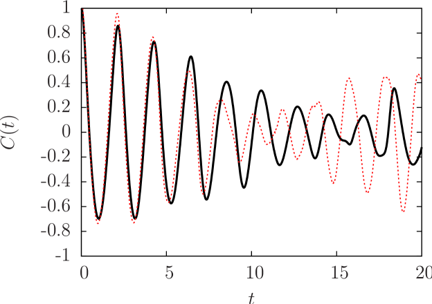
Figure 1: Part of the auto-correlation time-series used to extract spectral information for 2d harmonium in a magnetic field ($\omega_{L}=\omega_{0}=1$) and with Coulomb interaction. Solid line: full quantum, dotted line IVR semiclassical result.

We stress that without the Coulomb term the IVR results would be numerically exact and on top of the quantum ones (not shown). In the IVR case, with $\kappa=0$, even a single trajectory calculation according to the Thawed Gaussian approximation [33] is sufficient to generate the time-dependent semiclassical results. Therefore, the interesting case is the one with the Coulomb term.

For $\kappa=1$, the results for some eigenvalues extracted from the time-series shown above are listed in Table 2 and are compared to the corresponding WKB results.

$m$	WKB	IVR	QM
0	3.14	3.14	3.03
1	2.84	2.84	2.83
2	3.02	3.02	3.03

Table 2: Comparison of WKB energies for $n_{r}=0$ and different values of $m$ with those from semiclassical IVR and full quantum calculations, including the Coulomb interaction and for $\omega_{L}=\omega_{0}=1$.

We note that the IVR and WKB semiclassical results are coinciding to within the given accuracy, although in the time-dependent calculations we did not(!) employ any Langer correction of the potential. For single electron dynamics in the Coulomb potential the Langer correction, necessary in the energy domain [40], is needed in the time-domain if one uses non-Cartesian coordinates [41] and seems to be unnecessary for Cartesian coordinates [42, 43], which is corroborated here. Furthermore, with better than 1 percent accuracy both semiclassical results are lying on top of the full quantum result, except for the $m=0$ eigenvalue. In the specific case considered, the full quantum result is around 3 percent different from the semiclassical ones for $m=0$. Furthermore, by coincidence, for the present parameters, two quantum eigenvalues for $m=0$ and $m=2$ are degenerate. They do split up for a different choice of the ratio $\omega_{L}/\omega_{0}$, however, where a similar agreement between the differently calculated energy eigenvalues is found (not shown). The marked difference (a few percent) between the full quantum result for $m=0$ and the semiclassical ones does persist.

5 Conclusions and Outlook

We have shown that the time-dependent semiclassical IVR methodology of Herman and Kluk, based on Cartesian coordinates, is able to capture spectral features of two-electron quantum dots to a similar degree of accuracy as the WKB approach without the need to employ a Langer correction, complementing work on the comparison of WKB tunneling probabilities with Fourier transformed time-dependent semiclassical results [44, 45]. The semiclassical IVR method does not suffer from the restriction of WKB to integrable (e. g. one DOF) systems, however. This allows the investigation of non-circular quantum dots and also quantum dots in 3d or with more than two electrons. For the study of the dynamics of nuclear degrees of freedom the HK method, in the meantime, has become a widely used tool in the physics and chemistry communities (for an early review, see, e. g. [46]). An open question in the application to more than two-electron systems is the problem of anti-symmetrization of the wavefunction, however. Furthermore, we stress that there is no restriction on the value of $\Omega$, as is the case for the exact analytical solutions of the problem presented by Taut [5], where the sequence of admissible $\Omega$ starts with a value on the order of one and converges to zero.

References

References

- [1] H. Høgaasen, J.-M. Richard, and P. Sorba, Am. J. Phys. 78, 86 (2010).
- [2] N. R. Kestner and O. Sinanoglu, Phys. Rev. 128, 2687 (1962).
- [3] M. Taut, Phys. Rev. A 48, 3561 (1993).
- [4] A. Verçin, Phys. Lett. B 260, 120 (1991).
- [5] M. Taut, J. Phys. A 27, 1045 (1994).
- [6] A. Turbiner, Phys. Rev. A 50, 5335 (1994).
- [7] U. Merkt, J. Huser, and M. Wagner, Phys. Rev. A 43, 7320 (1991).
- [8] J. Cioslowski and K. Pernal, J. Chem. Phys. 113, 8434 (2000).
- [9] P.-F. Loos and P. M. W. Gill, Phys. Rev. Lett. 105, 113001 (2010).
- [10] T. Kramer, AIP Conference Proceedings 1323, 178 (2010).
- [11] R. Turton, The Quantum Dot: A Journey into Future Microelectronics (Oxford University Press, New York, 1995).
- [12] R. Rosas, R. Riera, J. L. Marín, and H. León, Am. J. Phys. 68, 835 (2000).
- [13] A. J. Larkoski, D. G. Ellis, and L. J. Curtis, Am. J. Phys. 74, 572 (2006).
- [14] S. Klama and E. G. Mishchenko, J. Phys.: Cond. Matt. 10, 3411 (1998).
- [15] R. G. Nazmitdinov, N. Simonovic, and J.-M. Rost, Phys. Rev. B 65, 155307 (2002).
- [16] E. J. Heller, J. Chem. Phys. 75, 2923 (1981).
- [17] M. F. Herman and E. Kluk, Chem. Phys. 91, 27 (1984).
- [18] K. G. Kay, J. Chem. Phys. 100, 4377 (1994).
- [19] E. J. Heller, Acc. Chem. Res. 14, 368 (1981).
- [20] C. Harabati and K. G. Kay, J. Chem. Phys. 127, 084104 (2007).
- [21] G. van de Sand and J.-M. Rost, Phys. Rev. A 62, 053403 (2000).
- [22] K. G. Kay, J. Chem. Phys. 100, 4432 (1994).
- [23] K. G. Kay, J. Chem. Phys. 101, 2250 (1994).
- [24] S. Curilef and F. Claro, Am. J. Phys. 65, 244 (1997).
- [25] F. Grossmann, Theoretical Femtosecond Physics: Atoms and Molecules in Strong Laser Fields (Springer, Berlin, Heidelberg, 2008).
- [26] S. K. Gray, D. W. Noid, and B. G. Sumpter, J. Chem. Phys. 101, 4062 (1994).
- [27] L. S. Schulman, Techniques and Applications of Path Integration (Dover, Mineola, 2005), pp. 22-26.
- [28] J. H. van Vleck, Proc. Acad. Nat. Sci. USA 14, 178 (1928).
- [29] M. C. Gutzwiller, J. Math. Phys. 8, 1979 (1967).
- [30] E. Kluk, M. F. Herman, and H. L. Davis, J. Chem. Phys. 84, 326 (1986).
- [31] C.-M. Goletz, F. Grossmann, and S. Tomsovic, Phys. Rev. E 80, 031101 (2009).
- [32] F. Grossmann and M. F. Herman, J. Phys. A: Math. Gen. 35, 9489 (2002).
- [33] E. J. Heller, J. Chem. Phys. 62, 1544 (1975).
- [34] V. Fock, Z. Phys. 47, 446 (1928).
- [35] C. G. Darwin, Proc. Cambridge Philos. Soc. 27, 86 (1931).
- [36] R. E. Langer, Phys. Rev. 51, 669 (1937).
- [37] F. Grossmann, V. A. Mandelshtam, H. S. Taylor, and J. S. Briggs, Chem. Phys. Lett. 279, 355 (1997).
- [38] I. Galbraith, Y. S. Ching, and E. Abraham, Am. J. Phys. 52, 60 (1984).
- [39] D. V. Shalashilin and M. S. Child, J. Chem. Phys. 122, 224108 (2005).
- [40] L. A. Young and G. E. Uhlenbeck, Phys. Rev. 36, 1154 (1930); M. V. Berry and K. E. Mount, Rep. Prog. Phys. 35, 315 (1972).
- [41] R. S. Manning and G. S. Ezra, Phys. Rev. A 50, 954 (1994).
- [42] I. M. Suarez Barnes, M. Nauenberg, M. Nockleby, and S. Tomsovic, J. Phys. A 27, 3299 (1994).
- [43] G. van de Sand and J.-M. Rost, Phys. Rev. A 59, R1723 (1999).
- [44] S. Keshavamurthy and W. H. Miller, Chem. Phys. Lett. 218, 189 (1994).
- [45] F. Grossmann and E. J. Heller, Chem. Phys. Lett. 241, 45 (1995).
- [46] F. Grossmann, Comm. At. Mol. Phys. 34, 141 (1999).