Randomized Dimensionality Reduction for k๐‘˜k-means Clustering

Christos Boutsidis
Yahoo Labs
New York, NY
boutsidis@yahoo-inc.com
โ€ƒโ€ƒ Anastasios Zouzias
Mathematical & Computational Sciences
IBM Zรผrich Research Lab
azo@zurich.ibm.com
โ€ƒโ€ƒ Michael W. Mahoney
Department of Statistics
UC Berkeley
mmahoney@stat.berkeley.edu
โ€ƒโ€ƒ Petros Drineas
Computer Science Department
Rensselaer Polytechnic Institute
drinep@cs.rpi.edu
Abstract

We study the topic of dimensionality reduction for k๐‘˜k-means clustering. Dimensionality reduction encompasses the union of two approaches: feature selection and feature extraction. A feature selection based algorithm for k๐‘˜k-means clustering selects a small subset of the input features and then applies k๐‘˜k-means clustering on the selected features. A feature extraction based algorithm for k๐‘˜k-means clustering constructs a small set of new artificial features and then applies k๐‘˜k-means clustering on the constructed features. Despite the significance of k๐‘˜k-means clustering as well as the wealth of heuristic methods addressing it, provably accurate feature selection methods for k๐‘˜k-means clustering are not known. On the other hand, two provably accurate feature extraction methods for k๐‘˜k-means clustering are known in the literature; one is based on random projections and the other is based on the singular value decomposition (SVD).

This paper makes further progress towards a better understanding of dimensionality reduction for k๐‘˜k-means clustering. Namely, we present the first provably accurate feature selection method for k๐‘˜k-means clustering and, in addition, we present two feature extraction methods. The first feature extraction method is based on random projections and it improves upon the existing results in terms of time complexity and number of features needed to be extracted. The second feature extraction method is based on fast approximate SVD factorizations and it also improves upon the existing results in terms of time complexity. The proposed algorithms are randomized and provide constant-factor approximation guarantees with respect to the optimal k๐‘˜k-means objective value.

1 Introduction

Clustering is ubiquitous in science and engineering with numerous application domains ranging from bio-informatics and medicine to the social sciences and the webย [20]. Perhaps the most well-known clustering algorithm is the so-called โ€œk๐‘˜k-meansโ€ algorithm or Lloydโ€™s method [26]. Lloydโ€™s method is an iterative expectation-maximization type approach that attempts to address the following objective: given a set of Euclidean points and a positive integer k๐‘˜k corresponding to the number of clusters, split the points into k๐‘˜k clusters so that the total sum of the squared Euclidean distances of each point to its nearest cluster center is minimized. Due to this intuitive objective as well as its effectivenessย [31], the Lloydโ€™s method for k๐‘˜k-means clustering has become enormously popular in applicationsย [35].

In recent years, the high dimensionality of modern massive datasets has provided a considerable challenge to the design of efficient algorithmic solutions for k๐‘˜k-means clustering. First, ultra-high dimensional data force existing algorithms for k๐‘˜k-means clustering to be computationally inefficient, and second, the existence of many irrelevant features may not allow the identification of the relevant underlying structure in the data [17]. Practitioners have addressed these obstacles by introducing feature selection and feature extraction techniques. Feature selection selects a (small) subset of the actual features of the data, whereas feature extraction constructs a (small) set of artificial features based on the original features. Here, we consider a rigorous approach to feature selection and feature extraction for k๐‘˜k-means clustering. Next, we describe the mathematical framework under which we will study such dimensionality reduction methods.

Consider m๐‘šm points ๐’ซ={๐ฉ1,๐ฉ2,โ€ฆ,๐ฉm}โŠ†โ„n๐’ซsubscript๐ฉ1subscript๐ฉ2โ€ฆsubscript๐ฉ๐‘šsuperscriptโ„๐‘›\mathcal{P}=\{{\mathbf{p}}_{1},{\mathbf{p}}_{2},\dots,{\mathbf{p}}_{m}\}\subseteq\R^{n} and an integer k๐‘˜k denoting the number of clusters. The objective of k๐‘˜k-means is to find a k๐‘˜k-partition of ๐’ซ๐’ซ\mathcal{P} such that points that are โ€œcloseโ€ to each other belong to the same cluster and points that are โ€œfarโ€ from each other belong to different clusters. A k๐‘˜k-partition of ๐’ซ๐’ซ\mathcal{P} is a collection ๐’ฎ={๐’ฎ1,๐’ฎ2,โ€ฆ,๐’ฎk}๐’ฎsubscript๐’ฎ1subscript๐’ฎ2โ€ฆsubscript๐’ฎ๐‘˜{\cal S}=\{\mathcal{S}_{1},\mathcal{S}_{2},\dots,\mathcal{S}_{k}\} of k๐‘˜k non-empty pairwise disjoint sets which covers ๐’ซ๐’ซ{\cal P}. Let sj=|๐’ฎj|subscript๐‘ ๐‘—subscript๐’ฎ๐‘—s_{j}=|\mathcal{S}_{j}| be the size of ๐’ฎjsubscript๐’ฎ๐‘—\mathcal{S}_{j} (j=1,2,โ€ฆ,k๐‘—12โ€ฆ๐‘˜j=1,2,\dots,k). For each set Sjsubscript๐‘†๐‘—S_{j}, let ๐jโˆˆโ„nsubscript๐๐‘—superscriptโ„๐‘›\bm{\mu}_{j}\in\R^{n} be its centroid:

๐j=โˆ‘๐ฉiโˆˆSj๐ฉisj.subscript๐๐‘—subscriptsubscript๐ฉ๐‘–subscript๐‘†๐‘—subscript๐ฉ๐‘–subscript๐‘ ๐‘—\bm{\mu}_{j}={\sum_{{\mathbf{p}}_{i}\in S_{j}}{\mathbf{p}}_{i}\over s_{j}}.

The k๐‘˜k-means objective function is

โ„ฑโ€‹(๐’ซ,๐’ฎ)=โˆ‘i=1mโ€–๐ฉiโˆ’๐โ€‹(๐ฉi)โ€–22,โ„ฑ๐’ซ๐’ฎsuperscriptsubscript๐‘–1๐‘šsuperscriptsubscriptnormsubscript๐ฉ๐‘–๐subscript๐ฉ๐‘–22\mathcal{F}(\mathcal{P},{\cal S})=\sum_{i=1}^{m}{\|{\mathbf{p}}_{i}-\bm{\mu}({\mathbf{p}}_{i})\|}_{2}^{2},

where ๐โ€‹(๐ฉi)โˆˆโ„n๐subscript๐ฉ๐‘–superscriptโ„๐‘›\bm{\mu}({\mathbf{p}}_{i})\in\R^{n} is the centroid of the cluster to which ๐ฉisubscript๐ฉ๐‘–{\mathbf{p}}_{i} belongs. The objective of k๐‘˜k-means clustering is to compute the optimal k๐‘˜k-partition of the points in ๐’ซ๐’ซ\mathcal{P},

๐’ฎoโ€‹pโ€‹t=argmin๐’ฎโ„ฑโ€‹(๐’ซ,๐’ฎ).subscript๐’ฎ๐‘œ๐‘๐‘กsubscriptargmin๐’ฎโ„ฑ๐’ซ๐’ฎ{\cal S}_{opt}=\mathop{\hbox{argmin}}\limits_{{\cal S}}{\cal F}(\mathcal{P},{\cal S}).

Now, the goal of dimensionality reduction for k๐‘˜k-means clustering is to construct points

๐’ซ^={๐ฉ^1,๐ฉ^2,โ€ฆ,๐ฉ^m}โŠ†โ„r^๐’ซsubscript^๐ฉ1subscript^๐ฉ2โ€ฆsubscript^๐ฉ๐‘šsuperscriptโ„๐‘Ÿ\mathcal{\hat{P}}=\{\hat{{\mathbf{p}}}_{1},\hat{{\mathbf{p}}}_{2},\dots,\hat{{\mathbf{p}}}_{m}\}\subseteq\R^{r}

(for some parameter rโ‰ชnmuch-less-than๐‘Ÿ๐‘›r\ll n) so that ๐’ซ^^๐’ซ\mathcal{\hat{P}} approximates the clustering structure of ๐’ซ๐’ซ\mathcal{P}. Dimensionality reduction via feature selection constructs the ๐ฉ^isubscript^๐ฉ๐‘–\hat{{\mathbf{p}}}_{i}โ€™s by selecting actual features of the corresponding ๐ฉisubscript๐ฉ๐‘–{\mathbf{p}}_{i}โ€™s, whereas dimensionality reduction via feature extraction constructs new artificial features based on the original features. More formally, assume that the optimum k๐‘˜k-means partition of the points in ๐’ซ^^๐’ซ\mathcal{\hat{P}} has been computed

๐’ฎ^oโ€‹pโ€‹t=argmin๐’ฎโ„ฑโ€‹(๐’ซ^,๐’ฎ).subscript^๐’ฎ๐‘œ๐‘๐‘กsubscriptargmin๐’ฎโ„ฑ^๐’ซ๐’ฎ\hat{{\cal S}}_{opt}=\mathop{\hbox{argmin}}\limits_{{\cal S}}{\cal F}(\mathcal{\hat{P}},{\cal S}).

A dimensionality reduction algorithm for k๐‘˜k-means clustering constructs a new set ๐’ซ^^๐’ซ\mathcal{\hat{P}} such that

โ„ฑโ€‹(๐’ซ,๐’ฎ^oโ€‹pโ€‹t)โ‰คฮณโ‹…โ„ฑโ€‹(๐’ซ,๐’ฎoโ€‹pโ€‹t)โ„ฑ๐’ซsubscript^๐’ฎ๐‘œ๐‘๐‘กโ‹…๐›พโ„ฑ๐’ซsubscript๐’ฎ๐‘œ๐‘๐‘ก{\cal F}(\mathcal{P},\hat{{\cal S}}_{opt})\leq\gamma\cdot{\cal F}(\mathcal{P},{\cal S}_{opt})

where ฮณ>0๐›พ0\gamma>0 is the approximation ratio of ๐’ฎ^oโ€‹pโ€‹tsubscript^๐’ฎ๐‘œ๐‘๐‘ก\hat{{\cal S}}_{opt}. In other words, we require that computing an optimal partition ๐’ฎ^oโ€‹pโ€‹tsubscript^๐’ฎ๐‘œ๐‘๐‘ก\hat{{\cal S}}_{opt} on the projected low-dimensional data and plugging it back to cluster the high dimensional data, will imply a ฮณ๐›พ\gamma factor approximation to the optimal clustering. Notice that we measure approximability by evaluating the k๐‘˜k-means objective function, which is a well studied approach in the literatureย [30, 24, 19, 18, 15, 31, 7]. Comparing the structure of the actual clusterings ๐’ฎ^oโ€‹pโ€‹tsubscript^๐’ฎ๐‘œ๐‘๐‘ก\hat{{\cal S}}_{opt} to ๐’ฎoโ€‹pโ€‹tsubscript๐’ฎ๐‘œ๐‘๐‘ก{\cal S}_{opt} would be much more interesting but our techniques do not seem to be helpful towards this direction. However, from an empirical point of viewย (see Sectionย 7), we do compare ๐’ฎ^oโ€‹pโ€‹tsubscript^๐’ฎ๐‘œ๐‘๐‘ก\hat{{\cal S}}_{opt} directly to ๐’ฎoโ€‹pโ€‹tsubscript๐’ฎ๐‘œ๐‘๐‘ก{\cal S}_{opt} observing favorable results.

Reference Description Dimensions Time = Oโ€‹(x),x=๐‘‚๐‘ฅ๐‘ฅabsentO(x),x= Approximation Ratio
Folklore RP Oโ€‹(logโก(m)/ฮต2)๐‘‚๐‘šsuperscript๐œ€2O(\log(m)/\varepsilon^{2}) mโ€‹nโ€‹โŒˆฮตโˆ’2โ€‹logโก(m)/logโก(n)โŒ‰๐‘š๐‘›superscript๐œ€2๐‘š๐‘›mn\lceil\varepsilon^{-2}\log(m)/\log(n)\rceil 1+ฮต1๐œ€1+\varepsilon
[12] Exact SVD k๐‘˜k mโ€‹nโ€‹minโก{m,n}๐‘š๐‘›๐‘š๐‘›mn\min\{m,n\} 222
[14] Exact SVD Oโ€‹(k/ฮต2)๐‘‚๐‘˜superscript๐œ€2O(k/\varepsilon^{2}) mโ€‹nโ€‹minโก{m,n}๐‘š๐‘›๐‘š๐‘›mn\min\{m,n\} 1+ฮต1๐œ€1+\varepsilon
Theoremย 11 RS Oโ€‹(kโ€‹logโก(k)/ฮต2)๐‘‚๐‘˜๐‘˜superscript๐œ€2O(k\log(k)/\varepsilon^{2}) mโ€‹nโ€‹k/ฮต๐‘š๐‘›๐‘˜๐œ€mnk/\varepsilon 3+ฮต3๐œ€3+\varepsilon
Theoremย 12 RP Oโ€‹(k/ฮต2)๐‘‚๐‘˜superscript๐œ€2O(k/\varepsilon^{2}) mโ€‹nโ€‹โŒˆฮตโˆ’2โ€‹k/logโก(n)โŒ‰๐‘š๐‘›superscript๐œ€2๐‘˜๐‘›mn\lceil\varepsilon^{-2}k/\log(n)\rceil 2+ฮต2๐œ€2+\varepsilon
Theoremย 13 Approx. SVD k๐‘˜k mโ€‹nโ€‹k/ฮต๐‘š๐‘›๐‘˜๐œ€mnk/\varepsilon 2+ฮต2๐œ€2+\varepsilon
Table 1: Provably accurate dimensionality reduction methods for k๐‘˜k-means clustering. RP stands for Random Projections, and RS stands for Random Sampling. The third column corresponds to the number of selected/extracted features; the fourth column corresponds to the time complexity of each dimensionality reduction method; the fifth column corresponds to the approximation ratio of each approach.

1.1 Prior Work

Despite the significance of dimensionality reduction in the context of clustering, as well as the wealth of heuristic methods addressing itย [16], to the best of our knowledge there are no provably accurate feature selection methods for k๐‘˜k-means clustering known. On the other hand, two provably accurate feature extraction methods are known in the literature that we describe next.

First, a result byย [23] indicates that one can construct r=Oโ€‹(logโก(m)/ฮต2)๐‘Ÿ๐‘‚๐‘šsuperscript๐œ€2r=O(\log(m)/\varepsilon^{2}) artificial features with Random Projections and, with high probability, obtain a (1+ฮต)1๐œ€(1+\varepsilon)-approximate clustering. The algorithm implied byย [23], which is a random-projection-type algorithm, is as follows: let ๐€โˆˆโ„mร—n๐€superscriptโ„๐‘š๐‘›{\mathbf{A}}\in\R^{m\times n} contain the points ๐’ซ={๐ฉ1,๐ฉ2,โ€ฆ,๐ฉm}โŠ†โ„n๐’ซsubscript๐ฉ1subscript๐ฉ2โ€ฆsubscript๐ฉ๐‘šsuperscriptโ„๐‘›\mathcal{P}=\{{\mathbf{p}}_{1},{\mathbf{p}}_{2},\dots,{\mathbf{p}}_{m}\}\subseteq\R^{n} as its rows; then, multiply ๐€๐€{\mathbf{A}} from the right with a random projection matrix ๐‘โˆˆโ„nร—r๐‘superscriptโ„๐‘›๐‘Ÿ{\mathbf{R}}\in\R^{n\times r} to construct ๐‚=๐€๐‘โˆˆโ„mร—r๐‚๐€๐‘superscriptโ„๐‘š๐‘Ÿ{\mathbf{C}}={\mathbf{A}}{\mathbf{R}}\in\R^{m\times r} containing the points ๐’ซ^={๐ฉ^1,๐ฉ^2,โ€ฆ,๐ฉ^m}โŠ†โ„r^๐’ซsubscript^๐ฉ1subscript^๐ฉ2โ€ฆsubscript^๐ฉ๐‘šsuperscriptโ„๐‘Ÿ\mathcal{\hat{P}}=\{\hat{{\mathbf{p}}}_{1},\hat{{\mathbf{p}}}_{2},\dots,\hat{{\mathbf{p}}}_{m}\}\subseteq\R^{r} as its rows (see Sectionย 3.2 for a definition of a random projection matrix). The proof of this result is immediate mainly due to the Johnson-Lindenstrauss lemmaย [23]. [23] proved that all the pairwise Euclidean distances of the points of ๐’ซ๐’ซ\mathcal{P} are preserved within a multiplicative factor 1ยฑฮตplus-or-minus1๐œ€1\pm\varepsilon. So, any value of the k๐‘˜k-means objective function, which depends only on pairwise distances of the points from the corresponding center point, is preserved within a factor 1ยฑฮตplus-or-minus1๐œ€1\pm\varepsilon in the reduced space.

Second, [12] argues that one can construct r=k๐‘Ÿ๐‘˜r=k artificial features using the SVD, in Oโ€‹(mโ€‹nโ€‹minโก{m,n})๐‘‚๐‘š๐‘›๐‘š๐‘›O(mn\min\{m,n\}) time, to obtain a 222-approximation on the clustering quality. The algorithm ofย [12] is as follows: given ๐€โˆˆโ„mร—n๐€superscriptโ„๐‘š๐‘›{\mathbf{A}}\in\R^{m\times n} containing the points of ๐’ซ๐’ซ\mathcal{P} and k๐‘˜k, construct ๐‚=๐€๐•kโˆˆโ„mร—k๐‚subscript๐€๐•๐‘˜superscriptโ„๐‘š๐‘˜{\mathbf{C}}={\mathbf{A}}{\mathbf{V}}_{k}\in\R^{m\times k}. Here, ๐•kโˆˆโ„nร—ksubscript๐•๐‘˜superscriptโ„๐‘›๐‘˜{\mathbf{V}}_{k}\in\R^{n\times k} contains the top k๐‘˜k right singular vectors of ๐€๐€{\mathbf{A}}. The proof of this result will be (briefly) discussed in Sectionsย 2.2 andย 6.

Finally, an extension of the latter SVD-type result (see Corollary 4.5 inย [14]) argues that Oโ€‹(k/ฮต2)๐‘‚๐‘˜superscript๐œ€2O(k/\varepsilon^{2}) dimensions (singular vectors) suffice for a relative-error approximation.

1.2 Summary of our Contributions

We present the first provably accurate feature selection algorithm for k๐‘˜k-means (Algorithmย 1). Namely, Theorem 11 presents an Oโ€‹(mโ€‹nโ€‹kโ€‹ฮตโˆ’1+kโ€‹logโก(k)โ€‹ฮตโˆ’2โ€‹logโก(kโ€‹logโก(k)โ€‹ฮตโˆ’1))๐‘‚๐‘š๐‘›๐‘˜superscript๐œ€1๐‘˜๐‘˜superscript๐œ€2๐‘˜๐‘˜superscript๐œ€1O(mnk\varepsilon^{-1}+k\log(k)\varepsilon^{-2}\log(k\log(k)\varepsilon^{-1})) time randomized algorithm that, with constant probability, achieves a (3+ฮต)3๐œ€(3+\varepsilon)-error with r=Oโ€‹(kโ€‹logโก(k)/ฮต2)๐‘Ÿ๐‘‚๐‘˜๐‘˜superscript๐œ€2r=O(k\log(k)/\varepsilon^{2}) features. Given ๐€๐€{\mathbf{A}} and k๐‘˜k, the algorithm of this theorem first computes ๐™โˆˆโ„nร—k๐™superscriptโ„๐‘›๐‘˜{\mathbf{Z}}\in\R^{n\times k}, which approximates ๐•kโˆˆโ„nร—ksubscript๐•๐‘˜superscriptโ„๐‘›๐‘˜{\mathbf{V}}_{k}\in\R^{n\times k} which contains the top k๐‘˜k right singular vectors of ๐€๐€{\mathbf{A}} 222[10] presented an unsupervised feature selection algorithm by working with the matrix ๐•ksubscript๐•๐‘˜{\mathbf{V}}_{k}; in this work, we show that the same approximation bound can be achieved by working with a matrix that approximates ๐•ksubscript๐•๐‘˜{\mathbf{V}}_{k} in the sense of low rank matrix approximations (see Lemmaย 4).. Then, the selection of the features (columns of ๐€๐€{\mathbf{A}}) is done with a standard randomized sampling approach with replacement with probabilities that are computed from the matrix ๐™๐™{\mathbf{Z}}. The proof of Theorem 11 is a synthesis of ideas fromย [12] andย [32], which study the paradigm of dimensionality reduction for k๐‘˜k-means clustering and the paradigm of randomized sampling, respectively.

Moreover, we describe a random-projection-type feature extraction algorithm: Theoremย 12 presents an Oโ€‹(mโ€‹nโ€‹โŒˆฮตโˆ’2โ€‹k/logโก(n)โŒ‰)๐‘‚๐‘š๐‘›superscript๐œ€2๐‘˜๐‘›O(mn\lceil\varepsilon^{-2}k/\log(n)\rceil) time algorithm that, with constant probability, achieves a (2+ฮต)2๐œ€(2+\varepsilon)-error with r=Oโ€‹(k/ฮต2)๐‘Ÿ๐‘‚๐‘˜superscript๐œ€2r=O(k/\varepsilon^{2}) artificial features. We improve the folklore result of the first row in Tableย 1 by means of showing that a smaller number of features are enough to obtain an approximate clustering. The algorithm of Theorem 12 is the same as with the one in the standard result for random projections that we outlined in the prior work section but uses only r=Oโ€‹(k/ฮต2)๐‘Ÿ๐‘‚๐‘˜superscript๐œ€2r=O(k/\varepsilon^{2}) dimensions for the random projection matrix. Our proof relies on ideas fromย [12] andย [33], which study the paradigm of dimension reduction for k๐‘˜k-means clustering and the paradigm of speeding up linear algebra problems, such as the low-rank matrix approximation problem, via random projections, respectively.

Finally, Theorem 13 describes a feature extraction algorithm that employs approximate SVD decompositions and constructs r=k๐‘Ÿ๐‘˜r=k artificial features in Oโ€‹(mโ€‹nโ€‹k/ฮต)๐‘‚๐‘š๐‘›๐‘˜๐œ€O(mnk/\varepsilon) time such that, with constant probability, the clustering error is at most a 2+ฮต2๐œ€2+\varepsilon multiplicative factor from the optimal. We improve the existing SVD dimensionality reduction method by showing that fast approximate SVD gives features that can do almost as well as the features from the exact SVD. Our algorithm and proof are similar to those inย [12], but we show that one only needs to compute an approximate SVD of ๐€๐€{\mathbf{A}}.

We summarize previous results as well as our results in Tableย 1.

2 Linear Algebraic Formulation and our Approach

2.1 Linear Algebraic Formulation of k๐‘˜k-means

From now on, we will switch to a linear algebraic formulation of the k๐‘˜k-means clustering problem following the notation used in the introduction. Define the data matrix ๐€โˆˆโ„mร—n๐€superscriptโ„๐‘š๐‘›{\mathbf{A}}\in\R^{m\times n} whose rows correspond to the data points,

๐€T=[๐ฉ1,โ€ฆ,๐ฉm]โˆˆโ„nร—m.superscript๐€Tsubscript๐ฉ1โ€ฆsubscript๐ฉ๐‘šsuperscriptโ„๐‘›๐‘š{\mathbf{A}}^{\textsc{T}}=[{\mathbf{p}}_{1},\ldots,{\mathbf{p}}_{m}]\in\R^{n\times m}.

We represent a k๐‘˜k-clustering ๐’ฎ๐’ฎ{\cal S} of ๐€๐€{\mathbf{A}} by its cluster indicator matrix ๐—โˆˆโ„mร—k๐—superscriptโ„๐‘š๐‘˜{\mathbf{X}}\in\R^{m\times k}. Each column j=1,โ€ฆ,k๐‘—1โ€ฆ๐‘˜j=1,\ldots,k of ๐—๐—{\mathbf{X}} corresponds to a cluster. Each row i=1,โ€ฆ,m๐‘–1โ€ฆ๐‘ši=1,\ldots,m indicates the cluster membership of the point ๐ฉiโˆˆโ„msubscript๐ฉ๐‘–superscriptโ„๐‘š{\mathbf{p}}_{i}\in\R^{m}. So, ๐—iโ€‹j=1/sjsubscript๐—๐‘–๐‘—1subscript๐‘ ๐‘—{\mathbf{X}}_{ij}=1/\sqrt{s_{j}} if and only if data point ๐ฉisubscript๐ฉ๐‘–{\mathbf{p}}_{i} is in cluster Sjsubscript๐‘†๐‘—S_{j}. Every row of ๐—๐—{\mathbf{X}} has exactly one non-zero element, corresponding to the cluster the data point belongs to. There are sjsubscript๐‘ ๐‘—s_{j} non-zero elements in column j๐‘—j which indicates the data points belonging to cluster Sjsubscript๐‘†๐‘—S_{j}. By slightly abusing notation, we define

โ„ฑโ€‹(๐€,๐—):=โ€‹โ€–๐€โˆ’๐—๐—Tโ€‹๐€โ€–F2.assignโ„ฑ๐€๐—superscriptsubscriptnorm๐€superscript๐—๐—T๐€F2\mathcal{F}({\mathbf{A}},{\mathbf{X}}):=\mbox{}\|{\mathbf{A}}-{\mathbf{X}}{\mathbf{X}}^{\textsc{T}}{\mathbf{A}}\|_{\mathrm{F}}^{2}.

Hence, for any cluster indicator matrix ๐—๐—{\mathbf{X}}, the following identities hold

โ„ฑโ€‹(๐€,๐—)=โˆ‘i=1mโ€–๐ฉiTโˆ’๐—iโ€‹๐—Tโ€‹๐€โ€–22=โˆ‘i=1mโ€–๐ฉiTโˆ’๐โ€‹(๐ฉi)Tโ€–22=โ„ฑโ€‹(๐’ซ,๐’ฎ),โ„ฑ๐€๐—superscriptsubscript๐‘–1๐‘šsuperscriptsubscriptnormsuperscriptsubscript๐ฉ๐‘–Tsubscript๐—๐‘–superscript๐—T๐€22superscriptsubscript๐‘–1๐‘šsuperscriptsubscriptnormsuperscriptsubscript๐ฉ๐‘–T๐superscriptsubscript๐ฉ๐‘–T22โ„ฑ๐’ซ๐’ฎ{\cal F}({\mathbf{A}},{\mathbf{X}})=\sum_{i=1}^{m}{\|{\mathbf{p}}_{i}^{\textsc{T}}-{\mathbf{X}}_{i}{\mathbf{X}}^{\textsc{T}}{\mathbf{A}}\|}_{2}^{2}=\sum_{i=1}^{m}{\|{\mathbf{p}}_{i}^{\textsc{T}}-\bm{\mu}({\mathbf{p}}_{i})^{\textsc{T}}\|}_{2}^{2}=\mathcal{F}(\mathcal{P},{\cal S}),

where we define ๐—isubscript๐—๐‘–{\mathbf{X}}_{i} as the i๐‘–ith row of ๐—๐—{\mathbf{X}} and we have used the identity ๐—iโ€‹๐—Tโ€‹๐€=๐โ€‹(pi)T,subscript๐—๐‘–superscript๐—T๐€๐superscriptsubscript๐‘๐‘–T{\mathbf{X}}_{i}{\mathbf{X}}^{\textsc{T}}{\mathbf{A}}=\bm{\mu}(p_{i})^{\textsc{T}}, for i=1,โ€ฆ,m๐‘–1โ€ฆ๐‘ši=1,...,m. This identity is true because ๐—Tโ€‹๐€superscript๐—T๐€{\mathbf{X}}^{\textsc{T}}{\mathbf{A}} is a matrix whose row j๐‘—j is sjโ€‹๐jsubscript๐‘ ๐‘—subscript๐๐‘—\sqrt{s_{j}}\bm{\mu}_{j}, proportional to the centroid of the j๐‘—jth cluster; now, ๐—isubscript๐—๐‘–{\mathbf{X}}_{i} picks the row corresponding to its non-zero element, i.e., the cluster corresponding to point i๐‘–i, and scales it by 1/sj1subscript๐‘ ๐‘—1/\sqrt{s_{j}}. In the above, ฮผโ€‹(๐ฉi)โˆˆโ„m๐œ‡subscript๐ฉ๐‘–superscriptโ„๐‘š\mu({\mathbf{p}}_{i})\in\R^{m} denotes the centroid of the cluster of which the point ๐ฉisubscript๐ฉ๐‘–{\mathbf{p}}_{i} belongs to. Using this formulation, the goal of k๐‘˜k-means is to find ๐—๐—{\mathbf{X}} which minimizes โ€‹โ€–๐€โˆ’๐—๐—Tโ€‹๐€โ€–F2superscriptsubscriptnorm๐€superscript๐—๐—T๐€F2\mbox{}\|{\mathbf{A}}-{\mathbf{X}}{\mathbf{X}}^{\textsc{T}}{\mathbf{A}}\|_{\mathrm{F}}^{2}.

To evaluate the quality of different clusterings, we will use the k๐‘˜k-means objective function. Given some clustering ๐—^^๐—\hat{\mathbf{X}}, we are interested in the ratio โ„ฑโ€‹(๐€,๐—^)/โ„ฑโ€‹(๐€,๐—opt),โ„ฑ๐€^๐—โ„ฑ๐€subscript๐—opt{\cal F}({\mathbf{A}},\hat{\mathbf{X}})/{\cal F}({\mathbf{A}},{\mathbf{X}}_{\mathrm{opt}}), where ๐—optsubscript๐—opt{\mathbf{X}}_{\mathrm{opt}} is an optimal clustering of ๐€๐€{\mathbf{A}}. The choice of evaluating a clustering under this framework is not new. In fact,ย [30, 24, 19, 18, 15, 31] provide results (other than dimensionality reduction methods) along the same lines. Below, we give the definition of the k๐‘˜k-means problem.

Definition 1.

[The k๐‘˜k-means clustering problem] Given ๐€โˆˆโ„mร—n๐€superscriptโ„๐‘š๐‘›{\mathbf{A}}\in\mathbb{R}^{m\times n} (representing m๐‘šm data points โ€“ rows โ€“ described with respect to n๐‘›n features โ€“ columns) and a positive integer k๐‘˜k denoting the number of clusters, find the indicator matrix ๐—optโˆˆโ„mร—ksubscript๐—optsuperscriptโ„๐‘š๐‘˜{\mathbf{X}}_{\mathrm{opt}}\in\R^{m\times k} which satisfies,

๐—opt=argmin๐—โˆˆ๐’ณโ€‹โ€–๐€โˆ’๐—๐—Tโ€‹๐€โ€–F2.subscript๐—optsubscriptargmin๐—๐’ณsuperscriptsubscriptnorm๐€superscript๐—๐—T๐€F2{\mathbf{X}}_{\mathrm{opt}}=\mathop{\hbox{argmin}}\limits_{{\mathbf{X}}\in\cal{X}}\mbox{}\|{\mathbf{A}}-{\mathbf{X}}{\mathbf{X}}^{\textsc{T}}{\mathbf{A}}\|_{\mathrm{F}}^{2}.

The optimal value of the k๐‘˜k-means clustering objective is

โ„ฑโ€‹(๐€,๐—opt)=min๐—โˆˆ๐’ณโกโ€‹โ€–๐€โˆ’๐—๐—Tโ€‹๐€โ€–F2=โ€‹โ€–๐€โˆ’๐—optโ€‹๐—optTโ€‹๐€โ€–F2=Fopt.โ„ฑ๐€subscript๐—optsubscript๐—๐’ณsuperscriptsubscriptnorm๐€superscript๐—๐—T๐€F2superscriptsubscriptnorm๐€subscript๐—optsuperscriptsubscript๐—optT๐€F2subscriptFopt{\cal F}({\mathbf{A}},{\mathbf{X}}_{\mathrm{opt}})=\min_{{\mathbf{X}}\in\cal{X}}\mbox{}\|{\mathbf{A}}-{\mathbf{X}}{\mathbf{X}}^{\textsc{T}}{\mathbf{A}}\|_{\mathrm{F}}^{2}=\mbox{}\|{\mathbf{A}}-{\mathbf{X}}_{\mathrm{opt}}{\mathbf{X}}_{\mathrm{opt}}^{\textsc{T}}{\mathbf{A}}\|_{\mathrm{F}}^{2}=\mathrm{F}_{\mathrm{opt}}.

In the above, ๐’ณ๐’ณ\cal{X} denotes the set of all mร—k๐‘š๐‘˜m\times k indicator matrices ๐—๐—{\mathbf{X}}.

Next, we formalize the notation of a โ€œk๐‘˜k-means approximation algorithmโ€.

Definition 2.

[k๐‘˜k-means approximation algorithm] An algorithm is called a โ€œฮณ๐›พ\gamma-approximationโ€ for the k๐‘˜k-means clustering problem (ฮณโ‰ฅ1๐›พ1\gamma\geq 1) if it takes inputs the dataset ๐€โˆˆโ„mร—n๐€superscriptโ„๐‘š๐‘›{\mathbf{A}}\in\R^{m\times n} and the number of clusters k๐‘˜k, and returns an indicator matrix ๐—ฮณโˆˆโ„mร—ksubscript๐—๐›พsuperscriptโ„๐‘š๐‘˜{\mathbf{X}}_{\gamma}\in\R^{m\times k} such that w.p. at least 1โˆ’ฮดฮณ1subscript๐›ฟ๐›พ1-\delta_{\gamma},

โ€‹โ€–๐€โˆ’๐—ฮณโ€‹๐—ฮณTโ€‹๐€โ€–F2โ‰คฮณโ€‹min๐—โˆˆ๐’ณโกโ€‹โ€–๐€โˆ’๐—๐—Tโ€‹๐€โ€–F2=ฮณโ‹…โ„ฑโ€‹(๐€,๐—opt)=ฮณโ‹…Fopt.superscriptsubscriptnorm๐€subscript๐—๐›พsuperscriptsubscript๐—๐›พT๐€F2๐›พsubscript๐—๐’ณsuperscriptsubscriptnorm๐€superscript๐—๐—T๐€F2โ‹…๐›พโ„ฑ๐€subscript๐—optโ‹…๐›พsubscriptFopt\mbox{}\|{\mathbf{A}}-{\mathbf{X}}_{\gamma}{\mathbf{X}}_{\gamma}^{\textsc{T}}{\mathbf{A}}\|_{\mathrm{F}}^{2}\leq\gamma\min_{{\mathbf{X}}\in\cal{X}}\mbox{}\|{\mathbf{A}}-{\mathbf{X}}{\mathbf{X}}^{\textsc{T}}{\mathbf{A}}\|_{\mathrm{F}}^{2}=\gamma\cdot{\cal F}({\mathbf{A}},{\mathbf{X}}_{\mathrm{opt}})=\gamma\cdot\mathrm{F}_{\mathrm{opt}}.

An example of such an approximation algorithm for k๐‘˜k-means is inย [24] with ฮณ=1+ฮต๐›พ1๐œ€\gamma=1+\varepsilon (0<ฮต<10๐œ€10<\varepsilon<1), and ฮดฮณsubscript๐›ฟ๐›พ\delta_{\gamma} a constant in (0,1)01(0,1). The corresponding running time is Oโ€‹(mโ€‹nโ‹…2(k/ฮต)Oโ€‹(1))๐‘‚โ‹…๐‘š๐‘›superscript2superscript๐‘˜๐œ€๐‘‚1O(mn\cdot 2^{(k/\varepsilon)^{O(1)}}).

Combining this algorithm (with ฮณ=1+ฮต๐›พ1๐œ€\gamma=1+\varepsilon) with, for example, our dimensionality reduction method in Sectionย 5, would result in an algorithm that preserves the clustering within a factor of 2+ฮต2๐œ€2+\varepsilon, for any ฮตโˆˆ(0,1/3)๐œ€013\varepsilon\in(0,1/3), and runs in total time Oโ€‹(mโ€‹nโ€‹โŒˆฮตโˆ’2โ€‹k/logโก(n)โŒ‰+kโ€‹nโ€‹2(k/ฮต)Oโ€‹(1)/ฮต2)๐‘‚๐‘š๐‘›superscript๐œ€2๐‘˜๐‘›๐‘˜๐‘›superscript2superscript๐‘˜๐œ€๐‘‚1superscript๐œ€2O(mn\lceil\varepsilon^{-2}k/\log(n)\rceil+kn2^{(k/\varepsilon)^{O(1)}}/\varepsilon^{2}). Compare this with the complexity of running this algorithm on the high dimensional data and notice that reducing the dimension from n๐‘›n to Oโ€‹(k/ฮต2)๐‘‚๐‘˜superscript๐œ€2O(k/\varepsilon^{2}) leads to a considerably faster algorithm. In practice though, the Lloyd algorithmย [26, 31] is very popular and although it does not admit a worst case theoretical analysis, it empirically does well. We thus employ the Lloyd algorithm for our experimental evaluation of our algorithms in Sectionย 7. Note that, after using, for example, the dimensionality reduction method in Sectionย 5, the cost of the Lloyd heuristic is only Oโ€‹(mโ€‹k2/ฮต2)๐‘‚๐‘šsuperscript๐‘˜2superscript๐œ€2O(mk^{2}/\varepsilon^{2}) per iteration. This should be compared to the cost of Oโ€‹(kโ€‹mโ€‹n)๐‘‚๐‘˜๐‘š๐‘›O(kmn) per iteration if applied on the original high dimensional data. Similar run time improvements arise if one uses the other dimension reduction algorithms proposed in this work.

2.2 Our Approach

The key insight of our work is to view the k๐‘˜k-means problem from the above linear algebraic perspective. In this setting, the data points are rows in a matrix ๐€๐€{\mathbf{A}} and feature selection corresponds to selection of a subset of columns from ๐€๐€{\mathbf{A}}. Also, feature extraction can be viewed as the construction of a matrix ๐‚๐‚{\mathbf{C}} which contains the constructed features. Our feature extraction algorithms are linear, i.e., the matrix ๐‚๐‚{\mathbf{C}} is of the form ๐‚=๐€๐ƒ๐‚๐€๐ƒ{\mathbf{C}}={\mathbf{A}}{\mathbf{D}}, for some matrix ๐ƒ๐ƒ{\mathbf{D}}; so, the columns in ๐‚๐‚{\mathbf{C}} are linear combinations of the columns of ๐€๐€{\mathbf{A}}, i.e., the new features are linear combinations of the original features.

Our work is inspired by the SVD feature extraction algorithm ofย [12], which also viewed the k๐‘˜k-means problem from a linear algebraic perspective. The main message of the result ofย [12] (see the algorithm and the analysis in Section 2 inย [12]) is that any matrix ๐‚๐‚{\mathbf{C}} which can be used to approximate the matrix ๐€๐€{\mathbf{A}} in some low-rank matrix approximation sense can also be used for dimensionality reduction in k๐‘˜k-means clustering. We will now present a short proof of this result to better understand its implications in our dimensionality reduction algorithms.

Given ๐€๐€{\mathbf{A}} and k๐‘˜k, the main algorithm ofย [12] constructs ๐‚=๐€๐•k๐‚subscript๐€๐•๐‘˜{\mathbf{C}}={\mathbf{A}}{\mathbf{V}}_{k}, where ๐•ksubscript๐•๐‘˜{\mathbf{V}}_{k} contains the top k๐‘˜k right singular vectors of ๐€๐€{\mathbf{A}}. Let ๐—oโ€‹pโ€‹tsubscript๐—๐‘œ๐‘๐‘ก{\mathbf{X}}_{opt} and ๐—^oโ€‹pโ€‹tsubscript^๐—๐‘œ๐‘๐‘ก\hat{{\mathbf{X}}}_{opt} be the cluster indicator matrices that corresponds to the optimum partition corresponding to the rows of ๐€๐€{\mathbf{A}} and the rows of ๐‚๐‚{\mathbf{C}}, respectively. In our setting for dimensionality reduction, we compare โ„ฑโ€‹(๐€,๐—^oโ€‹pโ€‹t)โ„ฑ๐€subscript^๐—๐‘œ๐‘๐‘ก{\cal F}({\mathbf{A}},\hat{{\mathbf{X}}}_{opt}) to โ„ฑโ€‹(๐€,๐—oโ€‹pโ€‹t)โ„ฑ๐€subscript๐—๐‘œ๐‘๐‘ก{\cal F}({\mathbf{A}},{\mathbf{X}}_{opt}). From the SVD of ๐€๐€{\mathbf{A}}, consider

๐€=๐€๐•kโ€‹๐•kTโŸ๐€k+๐€โˆ’๐€๐•kโ€‹๐•kTโŸ๐€ฯโˆ’k.๐€subscriptโŸsubscript๐€๐•๐‘˜superscriptsubscript๐•๐‘˜Tsubscript๐€๐‘˜subscriptโŸ๐€subscript๐€๐•๐‘˜superscriptsubscript๐•๐‘˜Tsubscript๐€๐œŒ๐‘˜{\mathbf{A}}=\underbrace{{\mathbf{A}}{\mathbf{V}}_{k}{\mathbf{V}}_{k}^{\textsc{T}}}_{{\mathbf{A}}_{k}}+\underbrace{{\mathbf{A}}-{\mathbf{A}}{\mathbf{V}}_{k}{\mathbf{V}}_{k}^{\textsc{T}}}_{{\mathbf{A}}_{\rho-k}}.

Also, notice that for any cluster indicator matrix ๐—^oโ€‹pโ€‹tsubscript^๐—๐‘œ๐‘๐‘ก\hat{{\mathbf{X}}}_{opt}

((๐ˆmโˆ’๐—^oโ€‹pโ€‹tโ€‹๐—^oโ€‹pโ€‹tT)โ€‹๐€k)โ€‹((๐ˆmโˆ’๐—^oโ€‹pโ€‹tโ€‹๐—^oโ€‹pโ€‹tT)โ€‹๐€ฯโˆ’k)T=๐ŸŽmร—m,subscript๐ˆ๐‘šsubscript^๐—๐‘œ๐‘๐‘กsuperscriptsubscript^๐—๐‘œ๐‘๐‘กTsubscript๐€๐‘˜superscriptsubscript๐ˆ๐‘šsubscript^๐—๐‘œ๐‘๐‘กsuperscriptsubscript^๐—๐‘œ๐‘๐‘กTsubscript๐€๐œŒ๐‘˜Tsubscript0๐‘š๐‘š\left(\left({\mathbf{I}}_{m}-\hat{{\mathbf{X}}}_{opt}\hat{{\mathbf{X}}}_{opt}^{\textsc{T}}\right){\mathbf{A}}_{k}\right)\left(\left({\mathbf{I}}_{m}-\hat{{\mathbf{X}}}_{opt}\hat{{\mathbf{X}}}_{opt}^{\textsc{T}}\right){\mathbf{A}}_{\rho-k}\right)^{\textsc{T}}={\bf 0}_{m\times m},

because ๐€kโ€‹๐€ฯโˆ’kT=๐ŸŽmร—msubscript๐€๐‘˜superscriptsubscript๐€๐œŒ๐‘˜Tsubscript0๐‘š๐‘š{\mathbf{A}}_{k}{\mathbf{A}}_{\rho-k}^{\textsc{T}}={\bf 0}_{m\times m}. Combining these two steps and by orthogonality, it follows that

โ€‹โ€–๐€โˆ’๐—^oโ€‹pโ€‹tโ€‹๐—^oโ€‹pโ€‹tTโ€‹๐€โ€–F2=โ€‹โ€–(๐ˆmโˆ’๐—^oโ€‹pโ€‹tโ€‹๐—^oโ€‹pโ€‹tT)โ€‹๐€kโ€–F2โŸฮธฮฑ2+โ€‹โ€–(๐ˆmโˆ’๐—^oโ€‹pโ€‹tโ€‹๐—^oโ€‹pโ€‹tT)โ€‹๐€ฯโˆ’kโ€–F2โŸฮธฮฒ2.superscriptsubscriptnorm๐€subscript^๐—๐‘œ๐‘๐‘กsuperscriptsubscript^๐—๐‘œ๐‘๐‘กT๐€F2subscriptโŸsuperscriptsubscriptnormsubscript๐ˆ๐‘šsubscript^๐—๐‘œ๐‘๐‘กsuperscriptsubscript^๐—๐‘œ๐‘๐‘กTsubscript๐€๐‘˜F2superscriptsubscript๐œƒ๐›ผ2subscriptโŸsuperscriptsubscriptnormsubscript๐ˆ๐‘šsubscript^๐—๐‘œ๐‘๐‘กsuperscriptsubscript^๐—๐‘œ๐‘๐‘กTsubscript๐€๐œŒ๐‘˜F2superscriptsubscript๐œƒ๐›ฝ2\mbox{}\|{\mathbf{A}}-\hat{{\mathbf{X}}}_{opt}\hat{{\mathbf{X}}}_{opt}^{\textsc{T}}{\mathbf{A}}\|_{\mathrm{F}}^{2}\ =\ \underbrace{\mbox{}\|({\mathbf{I}}_{m}-\hat{{\mathbf{X}}}_{opt}\hat{{\mathbf{X}}}_{opt}^{\textsc{T}}){\mathbf{A}}_{k}\|_{\mathrm{F}}^{2}}_{\theta_{\alpha}^{2}}\ +\ \underbrace{\mbox{}\|({\mathbf{I}}_{m}-\hat{{\mathbf{X}}}_{opt}\hat{{\mathbf{X}}}_{opt}^{\textsc{T}}){\mathbf{A}}_{\rho-k}\|_{\mathrm{F}}^{2}}_{\theta_{\beta}^{2}}.

We now bound the second term of the later equation. ๐ˆmโˆ’๐—^oโ€‹pโ€‹tโ€‹๐—^oโ€‹pโ€‹tTsubscript๐ˆ๐‘šsubscript^๐—๐‘œ๐‘๐‘กsuperscriptsubscript^๐—๐‘œ๐‘๐‘กT{\mathbf{I}}_{m}-\hat{{\mathbf{X}}}_{opt}\hat{{\mathbf{X}}}_{opt}^{\textsc{T}} is a projection matrix, so it can be dropped without increasing the Frobenius norm. Hence, by using this and the fact that ๐—optโ€‹๐—optTโ€‹๐€subscript๐—optsuperscriptsubscript๐—optT๐€{\mathbf{X}}_{\mathrm{opt}}{\mathbf{X}}_{\mathrm{opt}}^{\textsc{T}}{\mathbf{A}} has rank at most k๐‘˜k:

ฮธฮฒ2โ‰คโ€‹โ€–๐€ฯโˆ’kโ€–F2=โ€‹โ€–๐€โˆ’๐€kโ€–F2โ‰คโ€‹โ€–๐€โˆ’๐—optโ€‹๐—optTโ€‹๐€โ€–F2.superscriptsubscript๐œƒ๐›ฝ2superscriptsubscriptnormsubscript๐€๐œŒ๐‘˜F2superscriptsubscriptnorm๐€subscript๐€๐‘˜F2superscriptsubscriptnorm๐€subscript๐—optsuperscriptsubscript๐—optT๐€F2\theta_{\beta}^{2}\ \leq\ \mbox{}\|{\mathbf{A}}_{\rho-k}\|_{\mathrm{F}}^{2}\ =\mbox{}\|{\mathbf{A}}-{\mathbf{A}}_{k}\|_{\mathrm{F}}^{2}\ \leq\ \mbox{}\|{\mathbf{A}}-{\mathbf{X}}_{\mathrm{opt}}{\mathbf{X}}_{\mathrm{opt}}^{\textsc{T}}{\mathbf{A}}\|_{\mathrm{F}}^{2}.

From similar manipulations combined with the optimality of ๐—^oโ€‹pโ€‹tsubscript^๐—๐‘œ๐‘๐‘ก\hat{{\mathbf{X}}}_{opt}, it follows that

ฮธฮฑ2โ‰คโ€‹โ€–๐€โˆ’๐—optโ€‹๐—optTโ€‹๐€โ€–F2.superscriptsubscript๐œƒ๐›ผ2superscriptsubscriptnorm๐€subscript๐—optsuperscriptsubscript๐—optT๐€F2\theta_{\alpha}^{2}\ \leq\ \mbox{}\|{\mathbf{A}}-{\mathbf{X}}_{\mathrm{opt}}{\mathbf{X}}_{\mathrm{opt}}^{\textsc{T}}{\mathbf{A}}\|_{\mathrm{F}}^{2}.

Therefore, we conclude that โ„ฑโ€‹(๐€,๐—^oโ€‹pโ€‹t)โ‰ค2โ€‹โ„ฑโ€‹(๐€,๐—oโ€‹pโ€‹t)โ„ฑ๐€subscript^๐—๐‘œ๐‘๐‘ก2โ„ฑ๐€subscript๐—๐‘œ๐‘๐‘ก{\cal F}({\mathbf{A}},\hat{{\mathbf{X}}}_{opt})\leq 2{\cal F}({\mathbf{A}},{\mathbf{X}}_{opt}). The key insight in this approach is that ๐€k=๐€๐•kโ€‹๐•kT=๐‚โ‹…๐‡subscript๐€๐‘˜subscript๐€๐•๐‘˜superscriptsubscript๐•๐‘˜Tโ‹…๐‚๐‡{\mathbf{A}}_{k}={\mathbf{A}}{\mathbf{V}}_{k}{\mathbf{V}}_{k}^{\textsc{T}}={\mathbf{C}}\cdot{\mathbf{H}} (with ๐‡=๐•kT๐‡superscriptsubscript๐•๐‘˜T{\mathbf{H}}={\mathbf{V}}_{k}^{\textsc{T}}) and ๐€โˆ’๐‚๐‡=๐€ฯโˆ’k๐€๐‚๐‡subscript๐€๐œŒ๐‘˜{\mathbf{A}}-{\mathbf{C}}{\mathbf{H}}={\mathbf{A}}_{\rho-k}, which is the best rank k๐‘˜k approximation of ๐€๐€{\mathbf{A}} in the Frobenius norm (see Sectionย 3 for useful notation).

In all three methods of our work, we will construct matrices ๐‚=๐€๐ƒ๐‚๐€๐ƒ{\mathbf{C}}={\mathbf{A}}{\mathbf{D}}, for three different matrices ๐ƒ๐ƒ{\mathbf{D}}, such that ๐‚โ‹…๐‡โ‹…๐‚๐‡{\mathbf{C}}\cdot{\mathbf{H}}, for an appropriate ๐‡๐‡{\mathbf{H}}, is a good approximation to ๐€๐€{\mathbf{A}} with respect to the Frobenius norm, i.e., โ€‹โ€–๐€โˆ’๐‚โ‹…๐‡โ€–F2superscriptsubscriptnorm๐€โ‹…๐‚๐‡F2\mbox{}\|{\mathbf{A}}-{\mathbf{C}}\cdot{\mathbf{H}}\|_{\mathrm{F}}^{2} is roughly equal to โ€‹โ€–๐€โˆ’๐€kโ€–F2,superscriptsubscriptnorm๐€subscript๐€๐‘˜F2\mbox{}\|{\mathbf{A}}-{\mathbf{A}}_{k}\|_{\mathrm{F}}^{2}, where ๐€ksubscript๐€๐‘˜{\mathbf{A}}_{k} is the best rank k๐‘˜k matrix from the SVD of ๐€๐€{\mathbf{A}}. Then, replicating the above proof gives our main theorems. Notice that the above approach is a 222-approximation because ๐€k=๐‚โ‹…๐‡subscript๐€๐‘˜โ‹…๐‚๐‡{\mathbf{A}}_{k}={\mathbf{C}}\cdot{\mathbf{H}} is the best rank k๐‘˜k approximation to ๐€๐€{\mathbf{A}}; our algorithms will give a slightly worse error because our matrix ๐‚โ‹…๐‡โ‹…๐‚๐‡{\mathbf{C}}\cdot{\mathbf{H}} give an approximation which is slightly worse than the best rank k๐‘˜k approximation.

3 Preliminaries

Basic Notation.

We use ๐€,๐,โ€ฆ๐€๐โ€ฆ{\mathbf{A}},{\mathbf{B}},\dots to denote matrices; ๐š,๐ฉ,โ€ฆ๐š๐ฉโ€ฆ{\mathbf{a}},{\mathbf{p}},\dots to denote column vectors. ๐ˆnsubscript๐ˆ๐‘›{\mathbf{I}}_{n} is the nร—n๐‘›๐‘›n\times n identity matrix; ๐ŸŽmร—nsubscript0๐‘š๐‘›\bm{0}_{m\times n} is the mร—n๐‘š๐‘›m\times n matrix of zeros; ๐€(i)subscript๐€๐‘–{\mathbf{A}}_{(i)} is the i๐‘–i-th row of ๐€๐€{\mathbf{A}}; ๐€(j)superscript๐€๐‘—{\mathbf{A}}^{(j)} is the j๐‘—j-th column of ๐€๐€{\mathbf{A}}; and, ๐€iโ€‹jsubscript๐€๐‘–๐‘—{\mathbf{A}}_{ij} denotes the (i,j)๐‘–๐‘—(i,j)-th element of ๐€๐€{\mathbf{A}}. We use ๐”ผโกY๐”ผ๐‘Œ\operatorname{\mathbb{E}}{Y} to take the expectation of a random variable Y๐‘ŒY and โ„™(โ„ฐ)โ„™โ„ฐ\Prob({\cal E}) to take the probability of a probabilistic event โ„ฐโ„ฐ{\cal E}. We abbreviate โ€œindependent identically distributedโ€ to โ€œi.i.dโ€ and โ€œwith probabilityโ€ to โ€œw.pโ€.

Matrix norms.

We use the Frobenius and the spectral matrix norms: โ€‹โ€–๐€โ€–F=โˆ‘i,j๐€iโ€‹j2subscriptnorm๐€Fsubscript๐‘–๐‘—superscriptsubscript๐€๐‘–๐‘—2\mbox{}\|{\mathbf{A}}\|_{\mathrm{F}}=\sqrt{\sum_{i,j}{\mathbf{A}}_{ij}^{2}} and โ€‹โ€–๐€โ€–2=max๐ฑ:โ€‹โ€–๐ฑโ€–2=1โกโ€‹โ€–๐€๐ฑโ€–2subscriptnorm๐€2subscript:๐ฑsubscriptnorm๐ฑ21subscriptnorm๐€๐ฑ2\mbox{}\|{\mathbf{A}}\|_{2}=\max_{{\mathbf{x}}:\mbox{}\|{\mathbf{x}}\|_{2}=1}\mbox{}\|{\mathbf{A}}{\mathbf{x}}\|_{2}, respectively (for a matrix ๐€๐€{\mathbf{A}}). For any ๐€๐€{\mathbf{A}},๐๐{\mathbf{B}}: โ€‹โ€–๐€โ€–2โ‰คโ€‹โ€–๐€โ€–Fsubscriptnorm๐€2subscriptnorm๐€F\mbox{}\|{\mathbf{A}}\|_{2}\leq\mbox{}\|{\mathbf{A}}\|_{\mathrm{F}}, โ€‹โ€–๐€๐โ€–Fโ‰คโ€‹โ€–๐€โ€–Fโ€‹โ€‹โ€–๐โ€–2subscriptnorm๐€๐Fsubscriptnorm๐€Fsubscriptnorm๐2\mbox{}\|{\mathbf{A}}{\mathbf{B}}\|_{\mathrm{F}}\leq\mbox{}\|{\mathbf{A}}\|_{\mathrm{F}}\mbox{}\|{\mathbf{B}}\|_{2}, and โ€‹โ€–๐€๐โ€–Fโ‰คโ€‹โ€–๐€โ€–2โ€‹โ€‹โ€–๐โ€–Fsubscriptnorm๐€๐Fsubscriptnorm๐€2subscriptnorm๐F\mbox{}\|{\mathbf{A}}{\mathbf{B}}\|_{\mathrm{F}}\leq\mbox{}\|{\mathbf{A}}\|_{2}\mbox{}\|{\mathbf{B}}\|_{\mathrm{F}}. The latter two properties are stronger versions of the standard submultiplicativity property: โ€‹โ€–๐€๐โ€–Fโ‰คโ€‹โ€–๐€โ€–Fโ€‹โ€‹โ€–๐โ€–Fsubscriptnorm๐€๐Fsubscriptnorm๐€Fsubscriptnorm๐F\mbox{}\|{\mathbf{A}}{\mathbf{B}}\|_{\mathrm{F}}\leq\mbox{}\|{\mathbf{A}}\|_{\mathrm{F}}\mbox{}\|{\mathbf{B}}\|_{\mathrm{F}}. We will refer to these versions as spectral submultiplicativity. Finally, the triangle inequality of matrix norms indicates that โ€‹โ€–๐€+๐โ€–Fโ‰คโ€‹โ€–๐€โ€–F+โ€‹โ€–๐โ€–Fsubscriptnorm๐€๐Fsubscriptnorm๐€Fsubscriptnorm๐F\mbox{}\|{\mathbf{A}}+{\mathbf{B}}\|_{\mathrm{F}}\leq\mbox{}\|{\mathbf{A}}\|_{\mathrm{F}}+\mbox{}\|{\mathbf{B}}\|_{\mathrm{F}}.

Lemma 3 (Matrix Pythagorean Theorem).

Let ๐—,๐˜โˆˆโ„mร—n๐—๐˜superscriptโ„๐‘š๐‘›{\mathbf{X}},{\mathbf{Y}}\in\R^{m\times n} satisfy ๐—๐˜T=๐ŸŽmร—msuperscript๐—๐˜Tsubscript0๐‘š๐‘š{\mathbf{X}}{\mathbf{Y}}^{\textsc{T}}=\bm{0}_{m\times m}. Then,

โ€‹โ€–๐—+๐˜โ€–F2=โ€‹โ€–๐—โ€–F2+โ€‹โ€–๐˜โ€–F2.superscriptsubscriptnorm๐—๐˜F2superscriptsubscriptnorm๐—F2superscriptsubscriptnorm๐˜F2\mbox{}\|{\mathbf{X}}+{\mathbf{Y}}\|_{\mathrm{F}}^{2}=\mbox{}\|{\mathbf{X}}\|_{\mathrm{F}}^{2}+\mbox{}\|{\mathbf{Y}}\|_{\mathrm{F}}^{2}.
Proof.
โ€‹โ€–๐—+๐˜โ€–F2superscriptsubscriptnorm๐—๐˜F2\displaystyle\mbox{}\|{\mathbf{X}}+{\mathbf{Y}}\|_{\mathrm{F}}^{2} =\displaystyle= โ€‹๐“๐ซโ€‹((๐—+๐˜)โ€‹(๐—+๐˜)T)=โ€‹๐“๐ซโ€‹(๐—๐—T+๐—๐˜T+๐˜๐—T+๐˜๐˜T)๐“๐ซ๐—๐˜superscript๐—๐˜T๐“๐ซsuperscript๐—๐—Tsuperscript๐—๐˜Tsuperscript๐˜๐—Tsuperscript๐˜๐˜T\displaystyle\mbox{}{\bf{Tr}}\left(\left({\mathbf{X}}+{\mathbf{Y}}\right)\left({\mathbf{X}}+{\mathbf{Y}}\right)^{\textsc{T}}\right)=\mbox{}{\bf{Tr}}\left({\mathbf{X}}{\mathbf{X}}^{\textsc{T}}+{\mathbf{X}}{\mathbf{Y}}^{\textsc{T}}+{\mathbf{Y}}{\mathbf{X}}^{\textsc{T}}+{\mathbf{Y}}{\mathbf{Y}}^{\textsc{T}}\right)
=\displaystyle= โ€‹๐“๐ซโ€‹(๐—๐—T+๐ŸŽmร—m+๐ŸŽmร—m+๐˜๐˜T)=โ€‹๐“๐ซโ€‹(๐—Tโ€‹๐—)+โ€‹๐“๐ซโ€‹(๐˜๐˜T)๐“๐ซsuperscript๐—๐—Tsubscript0๐‘š๐‘šsubscript0๐‘š๐‘šsuperscript๐˜๐˜T๐“๐ซsuperscript๐—T๐—๐“๐ซsuperscript๐˜๐˜T\displaystyle\mbox{}{\bf{Tr}}\left({\mathbf{X}}{\mathbf{X}}^{\textsc{T}}+\bm{0}_{m\times m}+\bm{0}_{m\times m}+{\mathbf{Y}}{\mathbf{Y}}^{\textsc{T}}\right)=\mbox{}{\bf{Tr}}\left({\mathbf{X}}^{\textsc{T}}{\mathbf{X}}\right)+\mbox{}{\bf{Tr}}\left({\mathbf{Y}}{\mathbf{Y}}^{\textsc{T}}\right)
=\displaystyle= โ€‹โ€–๐—โ€–F2+โ€‹โ€–๐˜โ€–F2.superscriptsubscriptnorm๐—F2superscriptsubscriptnorm๐˜F2\displaystyle\mbox{}\|{\mathbf{X}}\|_{\mathrm{F}}^{2}+\mbox{}\|{\mathbf{Y}}\|_{\mathrm{F}}^{2}.

ย 

This matrix form of the Pythagorean theorem is the starting point for the proofs of the three main theorems presented in this work. The idea to use the Matrix Pythagorean theorem to analyze a dimensionality reduction method for k๐‘˜k-means was initially introduced inย [12] and it turns to be very useful to prove our results as well.

Singular Value Decomposition.

The SVD of ๐€โˆˆโ„mร—n๐€superscriptโ„๐‘š๐‘›{\mathbf{A}}\in\R^{m\times n} of rank ฯโ‰คminโก{m,n}๐œŒ๐‘š๐‘›\rho\leq\min\{m,n\} is ๐€=๐”๐€โ€‹๐šบ๐€โ€‹๐•๐€T๐€subscript๐”๐€subscript๐šบ๐€superscriptsubscript๐•๐€T{\mathbf{A}}={\mathbf{U}}_{{\mathbf{A}}}{\mathbf{\Sigma}}_{{\mathbf{A}}}{\mathbf{V}}_{\mathbf{A}}^{\textsc{T}}, with ๐”๐€โˆˆโ„mร—ฯ,subscript๐”๐€superscriptโ„๐‘š๐œŒ{\mathbf{U}}_{{\mathbf{A}}}\in\R^{m\times\rho}, ๐šบ๐€โˆˆโ„ฯร—ฯ,subscript๐šบ๐€superscriptโ„๐œŒ๐œŒ{\mathbf{\Sigma}}_{{\mathbf{A}}}\in\R^{\rho\times\rho}, and ๐•๐€โˆˆโ„nร—ฯsubscript๐•๐€superscriptโ„๐‘›๐œŒ{\mathbf{V}}_{\mathbf{A}}\in\R^{n\times\rho}. In some more details, the SVD of ๐€๐€{\mathbf{A}} is:

๐€=(๐”k๐”ฯโˆ’k)โŸ๐”๐€โˆˆโ„mร—ฯโ€‹(๐šบk๐ŸŽ๐ŸŽ๐šบฯโˆ’k)โŸ๐šบ๐€โˆˆโ„ฯร—ฯโ€‹(๐•kT๐•ฯโˆ’kT)โŸ๐•๐€Tโˆˆโ„ฯร—n,๐€subscriptโŸsubscript๐”๐‘˜subscript๐”๐œŒ๐‘˜subscript๐”๐€superscriptโ„๐‘š๐œŒsubscriptโŸsubscript๐šบ๐‘˜00subscript๐šบ๐œŒ๐‘˜subscript๐šบ๐€superscriptโ„๐œŒ๐œŒsubscriptโŸsuperscriptsubscript๐•๐‘˜Tsuperscriptsubscript๐•๐œŒ๐‘˜Tsuperscriptsubscript๐•๐€Tsuperscriptโ„๐œŒ๐‘›\displaystyle{\mathbf{A}}=\underbrace{\left(\begin{array}[]{cc}{\mathbf{U}}_{k}&{\mathbf{U}}_{\rho-k}\end{array}\right)}_{{\mathbf{U}}_{{\mathbf{A}}}\in\R^{m\times\rho}}\underbrace{\left(\begin{array}[]{cc}{\mathbf{\Sigma}}_{k}&\bf{0}\\ \bf{0}&{\mathbf{\Sigma}}_{\rho-k}\end{array}\right)}_{{\mathbf{\Sigma}}_{\mathbf{A}}\in\R^{\rho\times\rho}}\underbrace{\left(\begin{array}[]{c}{\mathbf{V}}_{k}^{\textsc{T}}\\ {\mathbf{V}}_{\rho-k}^{\textsc{T}}\end{array}\right)}_{{\mathbf{V}}_{\mathbf{A}}^{\textsc{T}}\in\R^{\rho\times n}},

with singular values ฯƒ1โ‰ฅโ€ฆโ‰ฅฯƒkโ‰ฅฯƒk+1โ‰ฅโ€ฆโ‰ฅฯƒฯ>0subscript๐œŽ1โ€ฆsubscript๐œŽ๐‘˜subscript๐œŽ๐‘˜1โ€ฆsubscript๐œŽ๐œŒ0\sigma_{1}\geq\ldots\geq\sigma_{k}\geq\sigma_{k+1}\geq\ldots\geq\sigma_{\rho}>0. We will use ฯƒiโ€‹(๐€)subscript๐œŽ๐‘–๐€\sigma_{i}\left({\mathbf{A}}\right) to denote the i๐‘–i-th singular value of ๐€๐€{\mathbf{A}} when the matrix is not clear from the context. The matrices ๐”kโˆˆโ„mร—ksubscript๐”๐‘˜superscriptโ„๐‘š๐‘˜{\mathbf{U}}_{k}\in\R^{m\times k} and ๐”ฯโˆ’kโˆˆโ„mร—(ฯโˆ’k)subscript๐”๐œŒ๐‘˜superscriptโ„๐‘š๐œŒ๐‘˜{\mathbf{U}}_{\rho-k}\in\R^{m\times(\rho-k)} contain the left singular vectors ofย ๐€๐€{\mathbf{A}}; and, similarly, the matrices ๐•kโˆˆโ„nร—ksubscript๐•๐‘˜superscriptโ„๐‘›๐‘˜{\mathbf{V}}_{k}\in\R^{n\times k} and ๐•ฯโˆ’kโˆˆโ„nร—(ฯโˆ’k)subscript๐•๐œŒ๐‘˜superscriptโ„๐‘›๐œŒ๐‘˜{\mathbf{V}}_{\rho-k}\in\R^{n\times(\rho-k)} contain the right singular vectors. ๐šบkโˆˆโ„kร—ksubscript๐šบ๐‘˜superscriptโ„๐‘˜๐‘˜{\mathbf{\Sigma}}_{k}\in\R^{k\times k} and ๐šบฯโˆ’kโˆˆโ„(ฯโˆ’k)ร—(ฯโˆ’k)subscript๐šบ๐œŒ๐‘˜superscriptโ„๐œŒ๐‘˜๐œŒ๐‘˜{\mathbf{\Sigma}}_{\rho-k}\in\R^{(\rho-k)\times(\rho-k)} contain the singular values ofย ๐€๐€{\mathbf{A}}. It is well-known that ๐€k=๐”kโ€‹๐šบkโ€‹๐•kT=๐€๐•kโ€‹๐•kT=๐”kโ€‹๐”kTโ€‹๐€subscript๐€๐‘˜subscript๐”๐‘˜subscript๐šบ๐‘˜superscriptsubscript๐•๐‘˜Tsubscript๐€๐•๐‘˜superscriptsubscript๐•๐‘˜Tsubscript๐”๐‘˜superscriptsubscript๐”๐‘˜T๐€{\mathbf{A}}_{k}={\mathbf{U}}_{k}{\mathbf{\Sigma}}_{k}{\mathbf{V}}_{k}^{\textsc{T}}={\mathbf{A}}{\mathbf{V}}_{k}{\mathbf{V}}_{k}^{\textsc{T}}={\mathbf{U}}_{k}{\mathbf{U}}_{k}^{\textsc{T}}{\mathbf{A}} minimizes โ€‹โ€–๐€โˆ’๐—โ€–Fsubscriptnorm๐€๐—F\mbox{}\|{\mathbf{A}}-{\mathbf{X}}\|_{\mathrm{F}} over all matrices ๐—โˆˆโ„mร—n๐—superscriptโ„๐‘š๐‘›{\mathbf{X}}\in\R^{m\times n} of rank at most kโ‰คฯ๐‘˜๐œŒk\leq\rho. We use ๐€ฯโˆ’k=๐€โˆ’๐€k=๐”ฯโˆ’kโ€‹๐šบฯโˆ’kโ€‹๐•ฯโˆ’kTsubscript๐€๐œŒ๐‘˜๐€subscript๐€๐‘˜subscript๐”๐œŒ๐‘˜subscript๐šบ๐œŒ๐‘˜superscriptsubscript๐•๐œŒ๐‘˜T{\mathbf{A}}_{\rho-k}={\mathbf{A}}-{\mathbf{A}}_{k}={\mathbf{U}}_{\rho-k}{\mathbf{\Sigma}}_{\rho-k}{\mathbf{V}}_{\rho-k}^{\textsc{T}}. Also, โ€‹โ€–๐€โ€–F=โˆ‘i=1ฯฯƒi2โ€‹(๐€)subscriptnorm๐€Fsuperscriptsubscript๐‘–1๐œŒsuperscriptsubscript๐œŽ๐‘–2๐€\mbox{}\|{\mathbf{A}}\|_{\mathrm{F}}=\sqrt{\sum_{i=1}^{\rho}\sigma_{i}^{2}({\mathbf{A}})} and โ€‹โ€–๐€โ€–2=ฯƒ1โ€‹(๐€)subscriptnorm๐€2subscript๐œŽ1๐€\mbox{}\|{\mathbf{A}}\|_{2}=\sigma_{1}({\mathbf{A}}). The best rank k๐‘˜k approximation to ๐€๐€{\mathbf{A}} also satisfies: โ€‹โ€–๐€โˆ’๐€kโ€–F=โˆ‘i=k+1ฯฯƒi2โ€‹(๐€)subscriptnorm๐€subscript๐€๐‘˜Fsuperscriptsubscript๐‘–๐‘˜1๐œŒsuperscriptsubscript๐œŽ๐‘–2๐€\mbox{}\|{\mathbf{A}}-{\mathbf{A}}_{k}\|_{\mathrm{F}}=\sqrt{\sum_{i=k+1}^{\rho}\sigma_{i}^{2}({\mathbf{A}})}.

Approximate Singular Value Decomposition.

The exact SVD of ๐€๐€{\mathbf{A}} takes cubic time. In this work, to speed up certain algorithms, we will use fast approximate SVD. We quote a recent result fromย [9], but similar relative-error Frobenius norm SVD approximations can be found elsewhere; see, for example,ย [33].

Lemma 4.

Given ๐€โˆˆโ„mร—n๐€superscriptโ„๐‘š๐‘›{\mathbf{A}}\in\R^{m\times n} of rank ฯ๐œŒ\rho, a target rank 2โ‰คk<ฯ2๐‘˜๐œŒ2\leq k<\rho, and 0<ฮต<10๐œ€10<\varepsilon<1, there exists a randomized algorithm that computes a matrix ๐™โˆˆโ„nร—k๐™superscriptโ„๐‘›๐‘˜{\mathbf{Z}}\in\R^{n\times k} such that ๐™Tโ€‹๐™=๐ˆksuperscript๐™T๐™subscript๐ˆ๐‘˜{\mathbf{Z}}^{\textsc{T}}{\mathbf{Z}}={\mathbf{I}}_{k}, ๐„๐™=๐ŸŽmร—k๐„๐™subscript0๐‘š๐‘˜{\mathbf{E}}{\mathbf{Z}}=\bm{0}_{m\times k} (for ๐„=๐€โˆ’๐€๐™๐™Tโˆˆโ„mร—n๐„๐€superscript๐€๐™๐™Tsuperscriptโ„๐‘š๐‘›{\mathbf{E}}={\mathbf{A}}-{\mathbf{A}}{\mathbf{Z}}{\mathbf{Z}}^{\textsc{T}}\in\R^{m\times n}), and

๐”ผโกโ€‹โ€–๐„โ€–F2โ‰ค(1+ฮต)โ€‹โ€‹โ€–๐€โˆ’๐€kโ€–F2.๐”ผsuperscriptsubscriptnorm๐„F21๐œ€superscriptsubscriptnorm๐€subscript๐€๐‘˜F2\operatorname{\mathbb{E}}{\mbox{}\|{\mathbf{E}}\|_{\mathrm{F}}^{2}}\leq\left(1+{\varepsilon}\right)\mbox{}\|{\mathbf{A}}-{\mathbf{A}}_{k}\|_{\mathrm{F}}^{2}.

The proposed algorithm runs in Oโ€‹(mโ€‹nโ€‹k/ฮต)๐‘‚๐‘š๐‘›๐‘˜๐œ€O\left(mnk/\varepsilon\right) time. We use ๐™=FastFrobeniusSVDโ€‹(๐€,k,ฮต)๐™FastFrobeniusSVD๐€๐‘˜๐œ€{\mathbf{Z}}=\text{FastFrobeniusSVD}({\mathbf{A}},k,\varepsilon) to denote this algorithm.

Notice that this lemma computes a rank-k๐‘˜k matrix ๐€๐™๐™Tsuperscript๐€๐™๐™T{\mathbf{A}}{\mathbf{Z}}{\mathbf{Z}}^{\textsc{T}} which, when is used to approximate ๐€๐€{\mathbf{A}}, is almost as good - in expectation - as the rank-k๐‘˜k matrix ๐€ksubscript๐€๐‘˜{\mathbf{A}}_{k} from the SVD of ๐€๐€{\mathbf{A}}. Since, ๐€k=๐€๐•kโ€‹๐•kTsubscript๐€๐‘˜subscript๐€๐•๐‘˜superscriptsubscript๐•๐‘˜T{\mathbf{A}}_{k}={\mathbf{A}}{\mathbf{V}}_{k}{\mathbf{V}}_{k}^{\textsc{T}}, the matrix ๐™๐™{\mathbf{Z}} is essentially an approximation of the matrix ๐•ksubscript๐•๐‘˜{\mathbf{V}}_{k} from the SVD of ๐€๐€{\mathbf{A}}.

We now give the details of the algorithm. The algorithm takes as inputs a matrix ๐€โˆˆโ„mร—n๐€superscriptโ„๐‘š๐‘›{\mathbf{A}}\in\R^{m\times n} of rank ฯ๐œŒ\rho and an integer 2โ‰คk<ฯ2๐‘˜๐œŒ2\leq k<\rho. Set r=k+โŒˆkฮต+1โŒ‰๐‘Ÿ๐‘˜๐‘˜๐œ€1r=k+{\left\lceil\,{k\over\varepsilon}+1\,\right\rceil} and construct ๐™๐™{\mathbf{Z}} with the following algorithm.

1:ย ย Generate an nร—r๐‘›๐‘Ÿn\times r standard Gaussian matrix ๐‘๐‘{\mathbf{R}} whose entries are i.i.d. ๐’ฉโ€‹(0,1)๐’ฉ01\mathcal{N}(0,1) variables.
2:ย ย ๐˜=๐€๐‘โˆˆโ„mร—r๐˜๐€๐‘superscriptโ„๐‘š๐‘Ÿ{\mathbf{Y}}={\mathbf{A}}{\mathbf{R}}\in\R^{m\times r}.
3:ย ย Orthonormalize the columns of ๐˜๐˜{\mathbf{Y}} to construct the matrix ๐โˆˆโ„mร—r๐superscriptโ„๐‘š๐‘Ÿ{\mathbf{Q}}\in\R^{m\times r}.
4:ย ย Let ๐™โˆˆโ„nร—k๐™superscriptโ„๐‘›๐‘˜{\mathbf{Z}}\in\R^{n\times k} be the top k๐‘˜k right singular vectors of ๐Tโ€‹๐€โˆˆโ„rร—nsuperscript๐T๐€superscriptโ„๐‘Ÿ๐‘›{\mathbf{Q}}^{\textsc{T}}{\mathbf{A}}\in\R^{r\times n}.

Pseudo-inverse.

๐€โ€ =๐•๐€โ€‹๐šบ๐€โˆ’1โ€‹๐”๐€Tโˆˆโ„nร—msuperscript๐€โ€ subscript๐•๐€superscriptsubscript๐šบ๐€1superscriptsubscript๐”๐€Tsuperscriptโ„๐‘›๐‘š{\mathbf{A}}^{\dagger}={\mathbf{V}}_{\mathbf{A}}{\mathbf{\Sigma}}_{\mathbf{A}}^{-1}{\mathbf{U}}_{\mathbf{A}}^{\textsc{T}}\in\R^{n\times m} denotes the so-called Moore-Penrose pseudo-inverse of ๐€๐€{\mathbf{A}} (here ๐šบ๐€โˆ’1superscriptsubscript๐šบ๐€1{\mathbf{\Sigma}}_{\mathbf{A}}^{-1} is the inverse of ๐šบ๐€subscript๐šบ๐€{\mathbf{\Sigma}}_{\mathbf{A}}), i.e., the unique nร—m๐‘›๐‘šn\times m matrix satisfying all four properties: ๐€=๐€๐€โ€ โ€‹๐€๐€superscript๐€๐€โ€ ๐€{\mathbf{A}}={\mathbf{A}}{\mathbf{A}}^{\dagger}{\mathbf{A}}, ๐€โ€ โ€‹๐€๐€โ€ =๐€โ€ superscript๐€โ€ superscript๐€๐€โ€ superscript๐€โ€ {\mathbf{A}}^{\dagger}{\mathbf{A}}{\mathbf{A}}^{\dagger}={\mathbf{A}}^{\dagger}, (๐€๐€โ€ )T=๐€๐€โ€ superscriptsuperscript๐€๐€โ€ Tsuperscript๐€๐€โ€ ({\mathbf{A}}{\mathbf{A}}^{\dagger})^{\textsc{T}}={\mathbf{A}}{\mathbf{A}}^{\dagger}, and (๐€โ€ โ€‹๐€)T=๐€โ€ โ€‹๐€superscriptsuperscript๐€โ€ ๐€Tsuperscript๐€โ€ ๐€({\mathbf{A}}^{\dagger}{\mathbf{A}})^{\textsc{T}}={\mathbf{A}}^{\dagger}{\mathbf{A}}. By the SVD of ๐€๐€{\mathbf{A}} and ๐€โ€ superscript๐€โ€ {\mathbf{A}}^{\dagger}, it is easy to verify that, for all i=1,โ€ฆ,ฯ=rankโ€‹(๐€)=rankโ€‹(๐€โ€ )formulae-sequence๐‘–1โ€ฆ๐œŒrank๐€ranksuperscript๐€โ€ i=1,\dots,\rho=\hbox{\rm rank}({\mathbf{A}})=\hbox{\rm rank}({\mathbf{A}}^{\dagger}): ฯƒiโ€‹(๐€โ€ )=1/ฯƒฯโˆ’i+1โ€‹(๐€)subscript๐œŽ๐‘–superscript๐€โ€ 1subscript๐œŽ๐œŒ๐‘–1๐€\sigma_{i}({\mathbf{A}}^{\dagger})=1/\sigma_{\rho-i+1}({\mathbf{A}}). Finally, for any ๐€โˆˆโ„mร—n,๐โˆˆโ„nร—โ„“formulae-sequence๐€superscriptโ„๐‘š๐‘›๐superscriptโ„๐‘›โ„“{\mathbf{A}}\in\R^{m\times n},{\mathbf{B}}\in\R^{n\times\ell}: (๐€๐)โ€ =๐โ€ โ€‹๐€โ€ superscript๐€๐โ€ superscript๐โ€ superscript๐€โ€ ({\mathbf{A}}{\mathbf{B}})^{\dagger}={\mathbf{B}}^{\dagger}{\mathbf{A}}^{\dagger} if any one of the following three properties hold: (i) ๐€Tโ€‹๐€=๐ˆnsuperscript๐€T๐€subscript๐ˆ๐‘›{\mathbf{A}}^{\textsc{T}}{\mathbf{A}}={\mathbf{I}}_{n}; (ii) ๐Tโ€‹๐=๐ˆโ„“superscript๐T๐subscript๐ˆโ„“{\mathbf{B}}^{\textsc{T}}{\mathbf{B}}={\mathbf{I}}_{\ell}; or, (iii) rankโ€‹(๐€)=rankโ€‹(๐)=nrank๐€rank๐๐‘›\hbox{\rm rank}({\mathbf{A}})=\hbox{\rm rank}({\mathbf{B}})=n.

Projection Matrices.

We call ๐โˆˆโ„nร—n๐superscriptโ„๐‘›๐‘›{\mathbf{P}}\in\R^{n\times n} a projection matrix if ๐2=๐superscript๐2๐{\mathbf{P}}^{2}={\mathbf{P}}. For such a projection matrix and any ๐€๐€{\mathbf{A}}: โ€‹โ€–๐๐€โ€–Fโ‰คโ€‹โ€–๐€โ€–F.subscriptnorm๐๐€Fsubscriptnorm๐€F\mbox{}\|{\mathbf{P}}{\mathbf{A}}\|_{\mathrm{F}}\leq\mbox{}\|{\mathbf{A}}\|_{\mathrm{F}}. Also, if ๐๐{\mathbf{P}} is a projection matrix, then, ๐ˆnโˆ’๐subscript๐ˆ๐‘›๐{\mathbf{I}}_{n}-{\mathbf{P}} is a projection matrix. So, for any matrix ๐€๐€{\mathbf{A}}, both ๐€๐€โ€ superscript๐€๐€โ€ {\mathbf{A}}{\mathbf{A}}^{\dagger} and ๐ˆnโˆ’๐€๐€โ€ subscript๐ˆ๐‘›superscript๐€๐€โ€ {\mathbf{I}}_{n}-{\mathbf{A}}{\mathbf{A}}^{\dagger} are projection matrices.

Markovโ€™s Inequality and the Union Bound.

Markovโ€™s inequality can be stated as follows: Let Y๐‘ŒY be a random variable taking non-negative values with expectation ๐”ผโกY๐”ผ๐‘Œ\operatorname{\mathbb{E}}{Y}. Then, for all t>0๐‘ก0t>0, and with probability at least 1โˆ’tโˆ’11superscript๐‘ก11-t^{-1}, Yโ‰คtโ‹…๐”ผโกY.๐‘Œโ‹…๐‘ก๐”ผ๐‘ŒY\leq t\cdot\operatorname{\mathbb{E}}{Y}. We will also use the so-called union bound. Given a set of probabilistic events โ„ฐ1,โ„ฐ2,โ€ฆ,โ„ฐnsubscriptโ„ฐ1subscriptโ„ฐ2โ€ฆsubscriptโ„ฐ๐‘›{\cal E}_{1},{\cal E}_{2},\ldots,{\cal E}_{n} holding with respective probabilities p1,p2,โ€ฆ,pnsubscript๐‘1subscript๐‘2โ€ฆsubscript๐‘๐‘›p_{1},p_{2},\ldots,p_{n}, the probability that all events hold simultaneously (a.k.a., the probability of the union of those events) is upper bounded as: โ„™(โ„ฐ1โˆชโ„ฐ2โ€‹โ€ฆโˆชโ„ฐn)โ‰คโˆ‘i=1npi.โ„™subscriptโ„ฐ1subscriptโ„ฐ2โ€ฆsubscriptโ„ฐ๐‘›superscriptsubscript๐‘–1๐‘›subscript๐‘๐‘–\Prob({\cal E}_{1}\cup{\cal E}_{2}\ldots\cup{\cal E}_{n})\leq\sum_{i=1}^{n}p_{i}.

3.1 Randomized Sampling

Sampling and Rescaling Matrices.

Let ๐€=[๐€(1),โ€ฆ,๐€(n)]โˆˆโ„mร—n๐€superscript๐€1โ€ฆsuperscript๐€๐‘›superscriptโ„๐‘š๐‘›{\mathbf{A}}=[{\mathbf{A}}^{(1)},\ldots,{\mathbf{A}}^{(n)}]\in\R^{m\times n} and let ๐‚=[๐€(i1),โ€ฆ,๐€(ir)]โˆˆโ„mร—r๐‚superscript๐€subscript๐‘–1โ€ฆsuperscript๐€subscript๐‘–๐‘Ÿsuperscriptโ„๐‘š๐‘Ÿ{\mathbf{C}}=[{\mathbf{A}}^{(i_{1})},\ldots,{\mathbf{A}}^{(i_{r})}]\in\R^{m\times r} consist of r<n๐‘Ÿ๐‘›r<n columns ofย ๐€๐€{\mathbf{A}}. Note that we can write ๐‚=๐€โ€‹๐›€๐‚๐€๐›€{\mathbf{C}}={\mathbf{A}}{\mathbf{\Omega}}, where the sampling matrix is ๐›€=[๐ži1,โ€ฆ,๐žir]โˆˆโ„nร—r๐›€subscript๐žsubscript๐‘–1โ€ฆsubscript๐žsubscript๐‘–๐‘Ÿsuperscriptโ„๐‘›๐‘Ÿ{\mathbf{\Omega}}=[{\mathbf{e}}_{i_{1}},\ldots,{\mathbf{e}}_{i_{r}}]\in\R^{n\times r} (here ๐žisubscript๐ž๐‘–{\mathbf{e}}_{i} are the standard basis vectors in โ„nsuperscriptโ„๐‘›\R^{n}). If ๐’โˆˆโ„rร—r๐’superscriptโ„๐‘Ÿ๐‘Ÿ{\mathbf{S}}\in\R^{r\times r} is a diagonal rescaling matrix then ๐€โ€‹๐›€โ€‹๐’๐€๐›€๐’{\mathbf{A}}{\mathbf{\Omega}}{\mathbf{S}} contains r๐‘Ÿr rescaled columns of ๐€๐€{\mathbf{A}}.

The following definition describes a simple randomized sampling procedure with replacement, which will be critical in our feature selection algorithm.

Definition 5 (Random Sampling with Replacement).

Let ๐—โˆˆโ„nร—k๐—superscriptโ„๐‘›๐‘˜{\mathbf{X}}\in\R^{n\times k} with n>k๐‘›๐‘˜n>k and let ๐—(i)subscript๐—๐‘–{\mathbf{X}}_{(i)} denote the i๐‘–i-th row of ๐—๐—{\mathbf{X}} as a row vector. For all i=1,โ€ฆ,n,๐‘–1โ€ฆ๐‘›i=1,\dots,n, define the following set of sampling probabilities:

pi=โ€‹โ€–๐—(i)โ€–22โ€‹โ€–๐—โ€–F2,subscript๐‘๐‘–superscriptsubscriptnormsubscript๐—๐‘–22superscriptsubscriptnorm๐—F2p_{i}={\mbox{}\|{\mathbf{X}}_{(i)}\|_{2}^{2}\over\mbox{}\|{\mathbf{X}}\|_{\mathrm{F}}^{2}},

and note that โˆ‘i=1npi=1superscriptsubscript๐‘–1๐‘›subscript๐‘๐‘–1\sum_{i=1}^{n}p_{i}=1. Let r๐‘Ÿr be a positive integer and construct the sampling matrix ๐›€โˆˆโ„nร—r๐›€superscriptโ„๐‘›๐‘Ÿ{\mathbf{\Omega}}\in\R^{n\times r} and the rescaling matrix ๐’โˆˆโ„rร—r๐’superscriptโ„๐‘Ÿ๐‘Ÿ{\mathbf{S}}\in\R^{r\times r} as follows: initially, ๐›€=๐ŸŽnร—r๐›€subscript0๐‘›๐‘Ÿ{\mathbf{\Omega}}=\bm{0}_{n\times r} and ๐’=๐ŸŽrร—r๐’subscript0๐‘Ÿ๐‘Ÿ{\mathbf{S}}=\bm{0}_{r\times r}; for t=1,โ€ฆ,r๐‘ก1โ€ฆ๐‘Ÿt=1,\dots,r pick an integer itsubscript๐‘–๐‘กi_{t} from the set {1,2,โ€ฆ,n}12โ€ฆ๐‘›\{1,2,\dots,n\} where the probability of picking i๐‘–i is equal to pisubscript๐‘๐‘–p_{i}; set ๐›€itโ€‹t=1subscript๐›€subscript๐‘–๐‘ก๐‘ก1{\mathbf{\Omega}}_{i_{t}t}=1 and ๐’tโ€‹t=1/rโ€‹pitsubscript๐’๐‘ก๐‘ก1๐‘Ÿsubscript๐‘subscript๐‘–๐‘ก{\mathbf{S}}_{tt}=1/\sqrt{rp_{i_{t}}}. We denote this randomized sampling technique with replacement by

[๐›€,๐’]=RandomizedSamplingโ€‹(๐—,r).๐›€๐’RandomizedSampling๐—๐‘Ÿ[{\mathbf{\Omega}},{\mathbf{S}}]=\text{RandomizedSampling}({\mathbf{X}},r).

Given ๐—๐—{\mathbf{X}} and r๐‘Ÿr, it takes Oโ€‹(nโ€‹k)๐‘‚๐‘›๐‘˜O(nk) time to compute the probabilities and another Oโ€‹(n+r)๐‘‚๐‘›๐‘ŸO(n+r) time to implement the sampling procedure via the technique inย [34]. In total, this method requires Oโ€‹(nโ€‹k)๐‘‚๐‘›๐‘˜O(nk) time.

The next three lemmas present the effect of the above sampling procedure on certain spectral properties, e.g. singular values, of orthogonal matrices. The first two lemmas are known; short proofs are included for the sake of completeness. The third lemma follows easily from the first two results (a proof of the lemma is given for completeness as well). We remind the reader that ฯƒi2โ€‹(๐—)superscriptsubscript๐œŽ๐‘–2๐—\sigma_{i}^{2}({\mathbf{X}}) denotes the i๐‘–ith singular value squared of the matrix ๐—๐—{\mathbf{X}}.

Lemmaย 6 argues that sampling and rescaling a sufficiently large number of rows from an orthonormal matrix with the randomized procedure of Definitionย 5 results in a matrix with singular values close to the singular values of the original orthonormal matrix.

Lemma 6.

Let ๐•โˆˆโ„nร—k๐•superscriptโ„๐‘›๐‘˜{\mathbf{V}}\in\R^{n\times k} with n>k๐‘›๐‘˜n>k and ๐•Tโ€‹๐•=๐ˆksuperscript๐•T๐•subscript๐ˆ๐‘˜{\mathbf{V}}^{\textsc{T}}{\mathbf{V}}={\mathbf{I}}_{k}. Let 0<ฮด<10๐›ฟ10<\delta<1, 4โ€‹kโ€‹lnโก(2โ€‹k/ฮด)<rโ‰คn4๐‘˜2๐‘˜๐›ฟ๐‘Ÿ๐‘›4k\ln(2k/\delta)<r\leq n, and [๐›€,๐’]=RandomizedSamplingโ€‹(๐•,r)๐›€๐’RandomizedSampling๐•๐‘Ÿ[{\mathbf{\Omega}},{\mathbf{S}}]=\text{RandomizedSampling}({\mathbf{V}},r). Then, for all i=1,โ€ฆ,k๐‘–1โ€ฆ๐‘˜i=1,\dots,k, w.p. at least 1โˆ’ฮด1๐›ฟ1-\delta,

1โˆ’4โ€‹kโ€‹lnโก(2โ€‹k/ฮด)rโ‰คฯƒi2โ€‹(๐•Tโ€‹๐›€โ€‹๐’)โ‰ค1+4โ€‹kโ€‹lnโก(2โ€‹k/ฮด)r.14๐‘˜2๐‘˜๐›ฟ๐‘Ÿsuperscriptsubscript๐œŽ๐‘–2superscript๐•T๐›€๐’14๐‘˜2๐‘˜๐›ฟ๐‘Ÿ1-\sqrt{{4k\ln(2k/\delta)\over r}}\leq\sigma_{i}^{2}({\mathbf{V}}^{\textsc{T}}{\mathbf{\Omega}}{\mathbf{S}})\leq 1+\sqrt{{4k\ln(2k/\delta)\over r}}.
Proof.

This result was originally proven in [32]. We will leverage a more recent proof of this result that appeared inย [27] and improves the original constants. More specifically, in Theorem 2 ofย [27], set ๐’=๐ˆ๐’๐ˆ{\mathbf{S}}={\mathbf{I}}, ฮฒ=1๐›ฝ1\beta=1, and replace ฮต๐œ€\varepsilon as a function of r๐‘Ÿr, ฮฒ๐›ฝ\beta, and d๐‘‘d to conclude the proof. ย 

Lemmaย 7 argues that sampling and rescaling columns from any matrix with the randomized procedure of Definitionย 5 results in a matrix with Frobenius norm squared close to the Frobenius norm squared of the original matrix. Intuitively, the subsampling of the columns does not affect much the Frobenius norm of the matrix.

Lemma 7.

For any rโ‰ฅ1๐‘Ÿ1r\geq 1, ๐—โˆˆโ„nร—k๐—superscriptโ„๐‘›๐‘˜{\mathbf{X}}\in\R^{n\times k}, and ๐˜โˆˆโ„mร—n๐˜superscriptโ„๐‘š๐‘›{\mathbf{Y}}\in\R^{m\times n}, let [๐›€,๐’]=RandomizedSamplingโ€‹(๐—,r)๐›€๐’RandomizedSampling๐—๐‘Ÿ[{\mathbf{\Omega}},{\mathbf{S}}]=\text{RandomizedSampling}({\mathbf{X}},r). Let ฮด๐›ฟ\delta be a parameter with 0<ฮด<10๐›ฟ10<\delta<1. Then, w.p. at least 1โˆ’ฮด1๐›ฟ1-\delta,

โ€‹โ€–๐˜โ€‹๐›€โ€‹๐’โ€–F2โ‰ค1ฮดโ€‹โ€‹โ€–๐˜โ€–F2.superscriptsubscriptnorm๐˜๐›€๐’F21๐›ฟsuperscriptsubscriptnorm๐˜F2\mbox{}\|{\mathbf{Y}}{\mathbf{\Omega}}{\mathbf{S}}\|_{\mathrm{F}}^{2}\leq{1\over\delta}\mbox{}\|{\mathbf{Y}}\|_{\mathrm{F}}^{2}.
Proof.

Define the random variable Y=โ€‹โ€–๐˜โ€‹๐›€โ€‹๐’โ€–F2โ‰ฅ0๐‘Œsuperscriptsubscriptnorm๐˜๐›€๐’F20Y=\mbox{}\|{\mathbf{Y}}{\mathbf{\Omega}}{\mathbf{S}}\|_{\mathrm{F}}^{2}\geq 0. Assume that the following equation is true: ๐”ผโกโ€‹โ€–๐˜โ€‹๐›€โ€‹๐’โ€–F2=โ€‹โ€–๐˜โ€–F2.๐”ผsuperscriptsubscriptnorm๐˜๐›€๐’F2superscriptsubscriptnorm๐˜F2\operatorname{\mathbb{E}}{\mbox{}\|{\mathbf{Y}}{\mathbf{\Omega}}{\mathbf{S}}\|_{\mathrm{F}}^{2}}=\mbox{}\|{\mathbf{Y}}\|_{\mathrm{F}}^{2}. Applying Markovโ€™s inequality with failure probability ฮด๐›ฟ\delta to this equation gives the bound in the lemma. All that remains to prove now is the above assumption. Let ๐=๐˜โ€‹๐›€โ€‹๐’โˆˆโ„mร—r,๐๐˜๐›€๐’superscriptโ„๐‘š๐‘Ÿ{\mathbf{B}}={\mathbf{Y}}{\mathbf{\Omega}}{\mathbf{S}}\in\R^{m\times r}, and for t=1,โ€ฆ,r,๐‘ก1โ€ฆ๐‘Ÿt=1,\dots,r, let ๐(t)superscript๐๐‘ก{\mathbf{B}}^{(t)} denotes the t๐‘กt-th column of ๐=๐˜โ€‹๐›€โ€‹๐’๐๐˜๐›€๐’{\mathbf{B}}={\mathbf{Y}}{\mathbf{\Omega}}{\mathbf{S}}. We manipulate the term ๐”ผโกโ€‹โ€–๐˜โ€‹๐›€โ€‹๐’โ€–F2๐”ผsuperscriptsubscriptnorm๐˜๐›€๐’F2\operatorname{\mathbb{E}}{\mbox{}\|{\mathbf{Y}}{\mathbf{\Omega}}{\mathbf{S}}\|_{\mathrm{F}}^{2}} as follows,

๐”ผโกโ€‹โ€–๐˜โ€‹๐›€โ€‹๐’โ€–F2=(a)๐”ผโ€‹โˆ‘t=1rโ€‹โ€–๐(t)โ€–22=(b)โˆ‘t=1r๐”ผโกโ€‹โ€–๐(t)โ€–22=(c)โˆ‘t=1rโˆ‘j=1npjโ€‹โ€‹โ€–๐˜(j)โ€–22rโ€‹pj=(d)1rโ€‹โˆ‘t=1rโ€‹โ€–๐˜โ€–F2=โ€‹โ€–๐˜โ€–F2superscript๐‘Ž๐”ผsuperscriptsubscriptnorm๐˜๐›€๐’F2๐”ผsuperscriptsubscript๐‘ก1๐‘Ÿsuperscriptsubscriptnormsuperscript๐๐‘ก22superscript๐‘superscriptsubscript๐‘ก1๐‘Ÿ๐”ผsuperscriptsubscriptnormsuperscript๐๐‘ก22superscript๐‘superscriptsubscript๐‘ก1๐‘Ÿsuperscriptsubscript๐‘—1๐‘›subscript๐‘๐‘—superscriptsubscriptnormsuperscript๐˜๐‘—22๐‘Ÿsubscript๐‘๐‘—superscript๐‘‘1๐‘Ÿsuperscriptsubscript๐‘ก1๐‘Ÿsuperscriptsubscriptnorm๐˜F2superscriptsubscriptnorm๐˜F2\displaystyle\operatorname{\mathbb{E}}{\mbox{}\|{\mathbf{Y}}{\mathbf{\Omega}}{\mathbf{S}}\|_{\mathrm{F}}^{2}}\buildrel(a)\over{=}\operatorname{\mathbb{E}}{\sum_{t=1}^{r}\mbox{}\|{\mathbf{B}}^{(t)}\|_{2}^{2}}\buildrel(b)\over{=}\sum_{t=1}^{r}\operatorname{\mathbb{E}}{\mbox{}\|{\mathbf{B}}^{(t)}\|_{2}^{2}}\buildrel(c)\over{=}\sum_{t=1}^{r}\sum_{j=1}^{n}p_{j}{\mbox{}\|{\mathbf{Y}}^{(j)}\|_{2}^{2}\over rp_{j}}\buildrel(d)\over{=}{1\over r}\sum_{t=1}^{r}\mbox{}\|{\mathbf{Y}}\|_{\mathrm{F}}^{2}=\mbox{}\|{\mathbf{Y}}\|_{\mathrm{F}}^{2}

(a)๐‘Ž(a) follows by the definition of the Frobenius norm of ๐๐{\mathbf{B}}. (b)๐‘(b) follows by the linearity of expectation. (c)๐‘(c) follows by our construction of ๐›€,๐’๐›€๐’{\mathbf{\Omega}},{\mathbf{S}}. (d)๐‘‘(d) follows by the definition of the Frobenius norm of ๐˜๐˜{\mathbf{Y}}. It is worth noting that the above manipulations hold for any set of probabilities since they cancel out in Equation (d)๐‘‘(d). ย 

Notice that ๐—๐—{\mathbf{X}} does not appear in the bound; it is only used as an input to the RandomizedSampling. This means that for any set of probabilities, a sampling and rescaling matrix constructed in the way it is described in Definitionย 5 satisfies the bound in the lemma.

The next lemma shows the effect of sub-sampling in a low-rank approximation of the form ๐€โ‰ˆ๐€๐™๐™T,๐€superscript๐€๐™๐™T{\mathbf{A}}\approx{\mathbf{A}}{\mathbf{Z}}{\mathbf{Z}}^{\textsc{T}}, where ๐™๐™{\mathbf{Z}} is a tall-and-skinny orthonormal matrix. The sub-sampling here is done on the columns of ๐€๐€{\mathbf{A}} and the corresponding rows of ๐™๐™{\mathbf{Z}}.

Lemma 8.

Fix ๐€โˆˆโ„mร—n๐€superscriptโ„๐‘š๐‘›{\mathbf{A}}\in\R^{m\times n}, kโ‰ฅ1๐‘˜1k\geq 1, 0<ฮต<1/30๐œ€130<\varepsilon<1/3, 0<ฮด<10๐›ฟ10<\delta<1, and r=4โ€‹kโ€‹lnโก(2โ€‹k/ฮด)/ฮต2๐‘Ÿ4๐‘˜2๐‘˜๐›ฟsuperscript๐œ€2r=4k\ln(2k/\delta)/\varepsilon^{2}. Compute the nร—k๐‘›๐‘˜n\times k matrix ๐™๐™{\mathbf{Z}} of Lemmaย 4 such that ๐€=๐€๐™๐™T+๐„๐€superscript๐€๐™๐™T๐„{\mathbf{A}}={\mathbf{A}}{\mathbf{Z}}{\mathbf{Z}}^{\textsc{T}}+{\mathbf{E}} and run [๐›€,๐’]=RandomizedSamplingโ€‹(๐™,r)๐›€๐’RandomizedSampling๐™๐‘Ÿ[{\mathbf{\Omega}},{\mathbf{S}}]=\text{RandomizedSampling}({\mathbf{Z}},r). Then, w.p. at least 1โˆ’3โ€‹ฮด13๐›ฟ1-3\delta, there exists ๐„~โˆˆโ„mร—n~๐„superscriptโ„๐‘š๐‘›\widetilde{{\mathbf{E}}}\in\R^{m\times n} such that

๐€๐™๐™T=๐€โ€‹๐›€โ€‹๐’โ€‹(๐™Tโ€‹๐›€โ€‹๐’)โ€ โ€‹๐™T+๐„~,superscript๐€๐™๐™T๐€๐›€๐’superscriptsuperscript๐™T๐›€๐’โ€ superscript๐™T~๐„{\mathbf{A}}{\mathbf{Z}}{\mathbf{Z}}^{\textsc{T}}={\mathbf{A}}{\mathbf{\Omega}}{\mathbf{S}}({\mathbf{Z}}^{\textsc{T}}{\mathbf{\Omega}}{\mathbf{S}})^{\dagger}{\mathbf{Z}}^{\textsc{T}}+\widetilde{{\mathbf{E}}},

and โ€‹โ€–๐„~โ€–Fโ‰ค1.6โ€‹ฮตฮดโ€‹โ€‹โ€–๐„โ€–F.subscriptnorm~๐„F1.6๐œ€๐›ฟsubscriptnorm๐„F\mbox{}\|\widetilde{{\mathbf{E}}}\|_{\mathrm{F}}\leq{1.6\varepsilon\over\sqrt{\delta}}\mbox{}\|{\mathbf{E}}\|_{\mathrm{F}}.

Proof.

See Appendix. ย 

In words, given ๐€๐€{\mathbf{A}} and the rank parameter k๐‘˜k, it is possible to construct two low rank matrices, ๐€๐™๐™Tsuperscript๐€๐™๐™T{\mathbf{A}}{\mathbf{Z}}{\mathbf{Z}}^{\textsc{T}} and ๐€โ€‹๐›€โ€‹๐’โ€‹(๐™Tโ€‹๐›€โ€‹๐’)โ€ โ€‹๐™T๐€๐›€๐’superscriptsuperscript๐™T๐›€๐’โ€ superscript๐™T{\mathbf{A}}{\mathbf{\Omega}}{\mathbf{S}}({\mathbf{Z}}^{\textsc{T}}{\mathbf{\Omega}}{\mathbf{S}})^{\dagger}{\mathbf{Z}}^{\textsc{T}} that are โ€œcloseโ€ to each other. Another way to view this result is that given the low-rank factorization ๐€๐™๐™Tsuperscript๐€๐™๐™T{\mathbf{A}}{\mathbf{Z}}{\mathbf{Z}}^{\textsc{T}} one can โ€œcompressโ€ ๐€๐€{\mathbf{A}} and ๐™๐™{\mathbf{Z}} by means of the sampling and rescaling matrices ๐›€๐›€{\mathbf{\Omega}} and ๐’.๐’{\mathbf{S}}. The error from such a compression will be bounded by ๐„~~๐„\tilde{{\mathbf{E}}}.

This result is useful in proving Theoremย 11 because at some point of the proof (see Eqn.ย (4)) we need to switch from a rank r๐‘Ÿr matrix (๐€โ€‹๐›€โ€‹๐’โ€‹(๐™Tโ€‹๐›€โ€‹๐’)โ€ โ€‹๐™T๐€๐›€๐’superscriptsuperscript๐™T๐›€๐’โ€ superscript๐™T{\mathbf{A}}{\mathbf{\Omega}}{\mathbf{S}}({\mathbf{Z}}^{\textsc{T}}{\mathbf{\Omega}}{\mathbf{S}})^{\dagger}{\mathbf{Z}}^{\textsc{T}}) to a rank k๐‘˜k matrix (๐€๐™๐™Tsuperscript๐€๐™๐™T{\mathbf{A}}{\mathbf{Z}}{\mathbf{Z}}^{\textsc{T}}) and at the same time keep the bounds in the resulting inequality almost unchanged (they would change by the norm of the matrix ๐„~~๐„\widetilde{{\mathbf{E}}}).

3.2 Random Projections

A classic result ofย [23] states that, for any 0<ฮต<10๐œ€10<\varepsilon<1, any set of m๐‘šm points in n๐‘›n dimensions (rows in ๐€โˆˆโ„mร—n๐€superscriptโ„๐‘š๐‘›{\mathbf{A}}\in\R^{m\times n}) can be linearly projected into

rฮต=Oโ€‹(logโก(m)/ฮต2)subscript๐‘Ÿ๐œ€๐‘‚๐‘šsuperscript๐œ€2r_{\varepsilon}=O\left(\log(m)/\varepsilon^{2}\right)

dimensions while preserving all the pairwise Euclidean distances of the points within a multiplicative factor of (1ยฑฮต)plus-or-minus1๐œ€(1\pm\varepsilon). More precisely,ย [23] showed the existence of a (random orthonormal) matrix ๐‘โˆˆโ„nร—rฮต๐‘superscriptโ„๐‘›subscript๐‘Ÿ๐œ€{\mathbf{R}}\in\R^{n\times r_{\varepsilon}} such that, for all i,j=1,โ€ฆ,mformulae-sequence๐‘–๐‘—1โ€ฆ๐‘ši,j=1,\dots,m, and with high probability (over the randomness of the matrix ๐‘๐‘{\mathbf{R}}),

(1โˆ’ฮต)โ€‹โ€–๐€(i)โˆ’๐€(j)โ€–2โ‰คโ€–(๐€(i)โˆ’๐€(j))โ€‹๐‘โ€–2โ‰ค(1+ฮต)โ€‹โ€–๐€(i)โˆ’๐€(j)โ€–2.1๐œ€subscriptnormsubscript๐€๐‘–subscript๐€๐‘—2subscriptnormsubscript๐€๐‘–subscript๐€๐‘—๐‘21๐œ€subscriptnormsubscript๐€๐‘–subscript๐€๐‘—2(1-\varepsilon){\|{\mathbf{A}}_{(i)}-{\mathbf{A}}_{(j)}\|}_{2}\leq{\|\left({\mathbf{A}}_{(i)}-{\mathbf{A}}_{(j)}\right){\mathbf{R}}\|}_{2}\leq(1+\varepsilon){\|{\mathbf{A}}_{(i)}-{\mathbf{A}}_{(j)}\|}_{2}.

Subsequent research simplified the proof ofย [23] by showing that such a linear transformation can be generated using a random Gaussian matrix, i.e., a matrix ๐‘โˆˆโ„nร—rฮต๐‘superscriptโ„๐‘›subscript๐‘Ÿ๐œ€{\mathbf{R}}\in\R^{n\times r_{\varepsilon}} whose entries are i.i.d. Gaussian random variables with zero mean and variance 1/r1๐‘Ÿ1/rย [22]. Recently,ย [5] presented the so-called Fast Johnson-Lindenstrauss Transform which describes an ๐‘โˆˆโ„nร—rฮต๐‘superscriptโ„๐‘›subscript๐‘Ÿ๐œ€{\mathbf{R}}\in\R^{n\times r_{\varepsilon}} such that the product ๐€๐‘๐€๐‘{\mathbf{A}}{\mathbf{R}} can be computed fast. In this paper, we will use a construction by [4], who proved that a rescaled random sign matrix, i.e., a matrix ๐‘โˆˆโ„nร—rฮต๐‘superscriptโ„๐‘›subscript๐‘Ÿ๐œ€{\mathbf{R}}\in\R^{n\times r_{\varepsilon}} whose entries have values {ยฑ1/r}plus-or-minus1๐‘Ÿ\{\pm 1/\sqrt{r}\} uniformly at random, satisfies the above equation. As we will see in detail in Sectionย 5, a recent result ofย [25] indicates that, if ๐‘๐‘{\mathbf{R}} is constructed as inย [4], the product ๐€๐‘๐€๐‘{\mathbf{A}}{\mathbf{R}} can be computed fast as well. We utilize such a random projection embedding in Section 5. Here, we summarize some properties of such matrices that might be of independent interest. We have deferred the proofs of the following lemmata to the Appendix.

The first lemma argues that the Frobenius norm squared of any matrix ๐˜๐˜{\mathbf{Y}} and the Frobenius norm squared of ๐˜๐‘,๐˜๐‘{\mathbf{Y}}{\mathbf{R}}, where ๐‘๐‘{\mathbf{R}} is a scaled signed matrix, are โ€œcomparableโ€. Lemmaย 9 is the analog of Lemmaย 7.

Lemma 9.

Fix any mร—n๐‘š๐‘›m\times n matrix ๐˜๐˜{\mathbf{Y}}, fix k>1๐‘˜1k>1 and ฮต>0๐œ€0\varepsilon>0. Let ๐‘โˆˆโ„nร—r๐‘superscriptโ„๐‘›๐‘Ÿ{\mathbf{R}}\in\R^{n\times r} be a rescaled random sign matrix constructed as described above with r=c0โ€‹k/ฮต2๐‘Ÿsubscript๐‘0๐‘˜superscript๐œ€2r=c_{0}k/\varepsilon^{2}, where c0โ‰ฅ100subscript๐‘0100c_{0}\geq 100. Then,

โ„™(โ€‹โ€–๐˜๐‘โ€–F2โ‰ฅ(1+ฮต)โ€‹โ€‹โ€–๐˜โ€–F2)โ‰ค0.01.โ„™superscriptsubscriptnorm๐˜๐‘F21๐œ€superscriptsubscriptnorm๐˜F20.01\Prob\left(\mbox{}\|{\mathbf{Y}}{\mathbf{R}}\|_{\mathrm{F}}^{2}\geq(1+\varepsilon)\mbox{}\|{\mathbf{Y}}\|_{\mathrm{F}}^{2}\right)\leq 0.01.

The next lemma argues about the effect of scaled random signed matrices to the singular values of orthonormal matrices.

Lemma 10.

Let ๐€โˆˆโ„mร—n๐€superscriptโ„๐‘š๐‘›{\mathbf{A}}\in\R^{m\times n} with rank ฯ๐œŒ\rho (k<ฯ๐‘˜๐œŒk<\rho), ๐€k=๐”kโ€‹๐šบkโ€‹๐•kTsubscript๐€๐‘˜subscript๐”๐‘˜subscript๐šบ๐‘˜superscriptsubscript๐•๐‘˜T{\mathbf{A}}_{k}={\mathbf{U}}_{k}{\mathbf{\Sigma}}_{k}{\mathbf{V}}_{k}^{\textsc{T}}, and 0<ฮต<1/30๐œ€130<\varepsilon<1/3. Let ๐‘โˆˆโ„nร—r๐‘superscriptโ„๐‘›๐‘Ÿ{\mathbf{R}}\in\R^{n\times r} be a (rescaled) random sign matrix constructed as we described above with r=c0โ€‹k/ฮต2๐‘Ÿsubscript๐‘0๐‘˜superscript๐œ€2r=c_{0}k/\varepsilon^{2}, where c0โ‰ฅ3330subscript๐‘03330c_{0}\geq 3330. The following hold (simultaneously) w.p. at least 0.970.970.97:

  1. 1.

    For all i=1,โ€ฆ,k๐‘–1โ€ฆ๐‘˜i=1,\dots,k:

    1โˆ’ฮตโ‰คฯƒi2โ€‹(๐•kTโ€‹๐‘)โ‰ค1+ฮต.1๐œ€superscriptsubscript๐œŽ๐‘–2superscriptsubscript๐•๐‘˜T๐‘1๐œ€1-\varepsilon\leq\sigma_{i}^{2}({\mathbf{V}}_{k}^{\textsc{T}}{\mathbf{R}})\leq 1+\varepsilon.
  2. 2.

    There exists an mร—n๐‘š๐‘›m\times n matrix ๐„~~๐„\widetilde{{\mathbf{E}}} such that

    ๐€k=๐€๐‘โ€‹(๐•kTโ€‹๐‘)โ€ โ€‹๐•kT+๐„~,subscript๐€๐‘˜๐€๐‘superscriptsuperscriptsubscript๐•๐‘˜T๐‘โ€ superscriptsubscript๐•๐‘˜T~๐„{\mathbf{A}}_{k}={\mathbf{A}}{\mathbf{R}}({\mathbf{V}}_{k}^{\textsc{T}}{\mathbf{R}})^{\dagger}{\mathbf{V}}_{k}^{\textsc{T}}+\widetilde{{\mathbf{E}}},

    and

    โ€‹โ€–๐„~โ€–Fโ‰ค3โ€‹ฮตโ€‹โ€‹โ€–๐€โˆ’๐€kโ€–F.subscriptnorm~๐„F3๐œ€subscriptnorm๐€subscript๐€๐‘˜F\mbox{}\|\widetilde{{\mathbf{E}}}\|_{\mathrm{F}}\leq 3\varepsilon\mbox{}\|{\mathbf{A}}-{\mathbf{A}}_{k}\|_{\mathrm{F}}.

The first statement of Lemmaย 10 is the analog of Lemmaย 6 while the second statement of Lemmaย 10 is the analog of Lemmaย 8. The results here replace the sampling and rescaling matrices ๐›€,๐’๐›€๐’{\mathbf{\Omega}},{\mathbf{S}} from Random Sampling (Definitionย 5) with the Random Projection matrix ๐‘๐‘{\mathbf{R}}. It is worth noting that almost the same results can be achieved with r=Oโ€‹(k/ฮต2)๐‘Ÿ๐‘‚๐‘˜superscript๐œ€2r=O(k/\varepsilon^{2}) random dimensions, while the corresponding lemmata for Random Sampling require at least r=Oโ€‹(kโ€‹logโกk/ฮต2)๐‘Ÿ๐‘‚๐‘˜๐‘˜superscript๐œ€2r=O(k\log k/\varepsilon^{2}) actual dimensions.

The second bound in the lemma is useful in proving Theoremย 12. Specifically, in Eqn.ย (12) we need to replace the rank k๐‘˜k matrix ๐€ksubscript๐€๐‘˜{\mathbf{A}}_{k} with another matrix of rank k๐‘˜k which is as close to ๐€ksubscript๐€๐‘˜{\mathbf{A}}_{k} as possible. The second bound above provides precisely such a matrix ๐€๐‘โ€‹(๐•kTโ€‹๐‘)โ€ โ€‹๐•kT๐€๐‘superscriptsuperscriptsubscript๐•๐‘˜T๐‘โ€ superscriptsubscript๐•๐‘˜T{\mathbf{A}}{\mathbf{R}}({\mathbf{V}}_{k}^{\textsc{T}}{\mathbf{R}})^{\dagger}{\mathbf{V}}_{k}^{\textsc{T}} with corresponding error ๐„~~๐„\widetilde{{\mathbf{E}}}.

Input: Dataset ๐€โˆˆโ„mร—n๐€superscriptโ„๐‘š๐‘›{\mathbf{A}}\in\R^{m\times n}, number of clusters k๐‘˜k, and 0<ฮต<1/30๐œ€130<\varepsilon<1/3.
Output: ๐‚โˆˆโ„mร—r๐‚superscriptโ„๐‘š๐‘Ÿ{\mathbf{C}}\in\R^{m\times r} with r=Oโ€‹(kโ€‹logโก(k)/ฮต2)๐‘Ÿ๐‘‚๐‘˜๐‘˜superscript๐œ€2r=O(k\log(k)/\varepsilon^{2}) rescaled features.
1:ย ย Let ๐™=FastFrobeniusSVDโ€‹(๐€,k,ฮต)๐™FastFrobeniusSVD๐€๐‘˜๐œ€{\mathbf{Z}}=\text{FastFrobeniusSVD}({\mathbf{A}},k,\varepsilon); ๐™โˆˆโ„nร—k๐™superscriptโ„๐‘›๐‘˜{\mathbf{Z}}\in\R^{n\times k} (via Lemmaย 4).
2:ย ย Let r=c1โ‹…4โ€‹kโ€‹lnโก(200โ€‹k)/ฮต2๐‘Ÿโ‹…subscript๐‘14๐‘˜200๐‘˜superscript๐œ€2r=c_{1}\cdot 4k\ln(200k)/\varepsilon^{2} (c1subscript๐‘1c_{1} is a sufficiently large constant - see proof).
3:ย ย Let [๐›€,๐’]=RandomizedSamplingโ€‹(๐™,r)๐›€๐’RandomizedSampling๐™๐‘Ÿ[{\mathbf{\Omega}},{\mathbf{S}}]=\text{RandomizedSampling}({\mathbf{Z}},r); ๐›€โˆˆโ„nร—r,๐’โˆˆโ„rร—rformulae-sequence๐›€superscriptโ„๐‘›๐‘Ÿ๐’superscriptโ„๐‘Ÿ๐‘Ÿ{\mathbf{\Omega}}\in\R^{n\times r},{\mathbf{S}}\in\R^{r\times r}(via Lemmaย 6).
4:ย ย Return ๐‚=๐€โ€‹๐›€โ€‹๐’โˆˆโ„mร—r๐‚๐€๐›€๐’superscriptโ„๐‘š๐‘Ÿ{\mathbf{C}}={\mathbf{A}}{\mathbf{\Omega}}{\mathbf{S}}\in\R^{m\times r} with r๐‘Ÿr rescaled columns from ๐€๐€{\mathbf{A}}.
Algorithmย 1 Randomized Feature Selection for k๐‘˜k-means Clustering.

4 Feature Selection with Randomized Sampling

Given ๐€,k๐€๐‘˜{\mathbf{A}},k, and 0<ฮต<1/30๐œ€130<\varepsilon<1/3, Algorithmย 1 is our main algorithm for feature selection in k๐‘˜k-means clustering. In a nutshell, construct the matrix ๐™๐™{\mathbf{Z}} with the (approximate) top-k๐‘˜k right singular vectors of ๐€๐€{\mathbf{A}} and select

r=Oโ€‹(kโ€‹logโก(k)/ฮต2)๐‘Ÿ๐‘‚๐‘˜๐‘˜superscript๐œ€2r=O(k\log(k)/\varepsilon^{2})

columns from ๐™Tsuperscript๐™T{\mathbf{Z}}^{\textsc{T}} with the randomized technique of Sectionย 3.1. One can replace the first step in Algorithmย 1 with the exact SVD of ๐€๐€{\mathbf{A}}ย [10]. The result that is obtained from this approach is asymptotically the same as the one we will present in Theoremย 11 333The main theorem of [10] states a (1+(1+ฮต)โ€‹ฮณ)11๐œ€๐›พ\left(1+(1+\varepsilon)\gamma\right)-approximation bound but the corresponding proof has a bug, which is fixable and leads to a (1+(2+ฮต)โ€‹ฮณ)12๐œ€๐›พ\left(1+(2+\varepsilon)\gamma\right)-approximation bound. One can replicate the corresponding (fixable) proof in [10] by replacing ๐™=๐•k๐™subscript๐•๐‘˜{\mathbf{Z}}={\mathbf{V}}_{k} in the proof of Theoremย 11 of our work.. Working with ๐™๐™{\mathbf{Z}} though gives a considerably faster algorithm.

Theorem 11.

Let ๐€โˆˆโ„mร—n๐€superscriptโ„๐‘š๐‘›{\mathbf{A}}\in\R^{m\times n} and k๐‘˜k be inputs of the k๐‘˜k-means clustering problem. Let ฮตโˆˆ(0,1/3)๐œ€013\varepsilon\in(0,1/3) and, by using Algorithmย 1 in Oโ€‹(mโ€‹nโ€‹k/ฮต+kโ€‹lnโก(k)/ฮต2โ€‹logโก(kโ€‹lnโก(k)/ฮต))๐‘‚๐‘š๐‘›๐‘˜๐œ€๐‘˜๐‘˜superscript๐œ€2๐‘˜๐‘˜๐œ€O(mnk/\varepsilon+k\ln(k)/\varepsilon^{2}\log(k\ln(k)/\varepsilon)) time construct features ๐‚โˆˆโ„mร—r๐‚superscriptโ„๐‘š๐‘Ÿ{\mathbf{C}}\in\R^{m\times r} with r=Oโ€‹(kโ€‹logโก(k)/ฮต2)๐‘Ÿ๐‘‚๐‘˜๐‘˜superscript๐œ€2r=O(k\log(k)/\varepsilon^{2}). Run any ฮณ๐›พ\gamma-approximation k๐‘˜k-means algorithm with failure probability ฮดฮณsubscript๐›ฟ๐›พ\delta_{\gamma} on ๐‚,k๐‚๐‘˜{\mathbf{C}},k and construct ๐—ฮณ~subscript๐—~๐›พ{\mathbf{X}}_{\tilde{\gamma}}. Then, w.p. at least 0.2โˆ’ฮดฮณ0.2subscript๐›ฟ๐›พ0.2-\delta_{\gamma},

โ€‹โ€–๐€โˆ’๐—ฮณ~โ€‹๐—ฮณ~Tโ€‹๐€โ€–F2โ‰ค(1+(2+ฮต)โ€‹ฮณ)โ€‹โ€‹โ€–๐€โˆ’๐—optโ€‹๐—optTโ€‹๐€โ€–F2.superscriptsubscriptnorm๐€subscript๐—~๐›พsuperscriptsubscript๐—~๐›พT๐€F212๐œ€๐›พsuperscriptsubscriptnorm๐€subscript๐—optsuperscriptsubscript๐—optT๐€F2\mbox{}\|{\mathbf{A}}-{\mathbf{X}}_{\tilde{\gamma}}{\mathbf{X}}_{\tilde{\gamma}}^{\textsc{T}}{\mathbf{A}}\|_{\mathrm{F}}^{2}\leq\left(1+(2+\varepsilon)\gamma\right)\mbox{}\|{\mathbf{A}}-{\mathbf{X}}_{\mathrm{opt}}{\mathbf{X}}_{\mathrm{opt}}^{\textsc{T}}{\mathbf{A}}\|_{\mathrm{F}}^{2}.

In words, given any set of points in some n๐‘›n-dimensional space and the number of clusters k๐‘˜k, it suffices to select roughly Oโ€‹(kโ€‹logโกk)๐‘‚๐‘˜๐‘˜O(k\log k) actual features from the given points and then run some k๐‘˜k-means algorithm on this subset of the input. The theorem formally argues that the clustering it would be obtained in the low-dimensional space will be close to the clustering it would have been obtained after running the k๐‘˜k-means method in the original high-dimensional data. We also state the result of the theorem in the notation we introduced in Sectionย 1,

โ„ฑโ€‹(๐’ซ,๐’ฎฮณ~)โ‰ค(1+(2+ฮต)โ€‹ฮณ)โ€‹โ„ฑโ€‹(๐’ซ,๐’ฎoโ€‹pโ€‹t).โ„ฑ๐’ซsubscript๐’ฎ~๐›พ12๐œ€๐›พโ„ฑ๐’ซsubscript๐’ฎ๐‘œ๐‘๐‘ก{\cal F}(\mathcal{P},{\cal S}_{\tilde{\gamma}})\leq\left(1+(2+\varepsilon)\gamma\right){\cal F}(\mathcal{P},{\cal S}_{opt}).

Here, ๐’ฎฮณ~subscript๐’ฎ~๐›พ{\cal S}_{\tilde{\gamma}} is the partition obtained after running the ฮณ๐›พ\gamma-approximation k๐‘˜k-means algorithm on the low-dimensional space. The approximation factor is (1+(2+ฮต)โ€‹ฮณ)12๐œ€๐›พ\left(1+(2+\varepsilon)\gamma\right). The term ฮณ>1๐›พ1\gamma>1 is due to the fact that the k๐‘˜k-means method that we run in the low-dimensional space does not recover the optimal k๐‘˜k-means partition. The other factor 2+ฮต2๐œ€2+\varepsilon is due to the fact that we run k๐‘˜k-means in the low-dimensional space.

Proof.

(of Theoremย 11) We start by manipulating the term โ€‹โ€–๐€โˆ’๐—ฮณ~โ€‹๐—ฮณ~Tโ€‹๐€โ€–F2superscriptsubscriptnorm๐€subscript๐—~๐›พsuperscriptsubscript๐—~๐›พT๐€F2\mbox{}\|{\mathbf{A}}-{\mathbf{X}}_{\tilde{\gamma}}{\mathbf{X}}_{\tilde{\gamma}}^{\textsc{T}}{\mathbf{A}}\|_{\mathrm{F}}^{2}. Notice that ๐€=๐€๐™๐™T+๐„๐€superscript๐€๐™๐™T๐„{\mathbf{A}}={\mathbf{A}}{\mathbf{Z}}{\mathbf{Z}}^{\textsc{T}}+{\mathbf{E}} (from Lemmaย 4). Also,

((๐ˆmโˆ’๐—ฮณ~โ€‹๐—ฮณ~T)โ€‹๐€๐™๐™T)โ€‹((๐ˆmโˆ’๐—ฮณ~โ€‹๐—ฮณ~T)โ€‹๐„)T=๐ŸŽmร—m,subscript๐ˆ๐‘šsubscript๐—~๐›พsuperscriptsubscript๐—~๐›พTsuperscript๐€๐™๐™Tsuperscriptsubscript๐ˆ๐‘šsubscript๐—~๐›พsuperscriptsubscript๐—~๐›พT๐„Tsubscript0๐‘š๐‘š\left(\left({\mathbf{I}}_{m}-{\mathbf{X}}_{\tilde{\gamma}}{\mathbf{X}}_{\tilde{\gamma}}^{\textsc{T}}\right){\mathbf{A}}{\mathbf{Z}}{\mathbf{Z}}^{\textsc{T}}\right)\left(\left({\mathbf{I}}_{m}-{\mathbf{X}}_{\tilde{\gamma}}{\mathbf{X}}_{\tilde{\gamma}}^{\textsc{T}}\right){\mathbf{E}}\right)^{\textsc{T}}={\bf 0}_{m\times m},

because ๐™Tโ€‹๐„T=๐ŸŽkร—msuperscript๐™Tsuperscript๐„Tsubscript0๐‘˜๐‘š{\mathbf{Z}}^{\textsc{T}}{\mathbf{E}}^{\textsc{T}}={\bf 0}_{k\times m}, by construction. Now, using Matrix Pythagoras (see Lemmaย 3),

โ€‹โ€–๐€โˆ’๐—ฮณ~โ€‹๐—ฮณ~Tโ€‹๐€โ€–F2=โ€‹โ€–(๐ˆmโˆ’๐—ฮณ~โ€‹๐—ฮณ~T)โ€‹๐€๐™๐™Tโ€–F2โŸฮธ12+โ€‹โ€–(๐ˆmโˆ’๐—ฮณ~โ€‹๐—ฮณ~T)โ€‹๐„โ€–F2โŸฮธ22.superscriptsubscriptnorm๐€subscript๐—~๐›พsuperscriptsubscript๐—~๐›พT๐€F2subscriptโŸsuperscriptsubscriptnormsubscript๐ˆ๐‘šsubscript๐—~๐›พsuperscriptsubscript๐—~๐›พTsuperscript๐€๐™๐™TF2superscriptsubscript๐œƒ12subscriptโŸsuperscriptsubscriptnormsubscript๐ˆ๐‘šsubscript๐—~๐›พsuperscriptsubscript๐—~๐›พT๐„F2superscriptsubscript๐œƒ22\displaystyle\mbox{}\|{\mathbf{A}}-{\mathbf{X}}_{\tilde{\gamma}}{\mathbf{X}}_{\tilde{\gamma}}^{\textsc{T}}{\mathbf{A}}\|_{\mathrm{F}}^{2}=\underbrace{\mbox{}\|({\mathbf{I}}_{m}-{\mathbf{X}}_{\tilde{\gamma}}{\mathbf{X}}_{\tilde{\gamma}}^{\textsc{T}}){\mathbf{A}}{\mathbf{Z}}{\mathbf{Z}}^{\textsc{T}}\|_{\mathrm{F}}^{2}}_{\theta_{1}^{2}}+\underbrace{\mbox{}\|({\mathbf{I}}_{m}-{\mathbf{X}}_{\tilde{\gamma}}{\mathbf{X}}_{\tilde{\gamma}}^{\textsc{T}}){\mathbf{E}}\|_{\mathrm{F}}^{2}}_{\theta_{2}^{2}}. (2)

We first bound the second term of Eqn.ย (2). Since ๐ˆmโˆ’๐—ฮณ~โ€‹๐—ฮณ~Tsubscript๐ˆ๐‘šsubscript๐—~๐›พsuperscriptsubscript๐—~๐›พT{\mathbf{I}}_{m}-{\mathbf{X}}_{\tilde{\gamma}}{\mathbf{X}}_{\tilde{\gamma}}^{\textsc{T}} is a projection matrix, it can be dropped without increasing the Frobenius norm (see Sectionย 3). Applying Markovโ€™s inequality on the equation of Lemmaย 4, we obtain that w.p. 0.990.990.99,

โ€‹โ€–๐„โ€–F2โ‰ค(1+100โ€‹ฮต)โ€‹โ€‹โ€–๐€โˆ’๐€kโ€–F2.superscriptsubscriptnorm๐„F21100๐œ€superscriptsubscriptnorm๐€subscript๐€๐‘˜F2\mbox{}\|{\mathbf{E}}\|_{\mathrm{F}}^{2}\leq(1+100\varepsilon)\mbox{}\|{\mathbf{A}}-{\mathbf{A}}_{k}\|_{\mathrm{F}}^{2}. (3)

(See the Appendix for a short proof of this statement.) Note also that ๐—optโ€‹๐—optTโ€‹๐€subscript๐—optsuperscriptsubscript๐—optT๐€{\mathbf{X}}_{\mathrm{opt}}{\mathbf{X}}_{\mathrm{opt}}^{\textsc{T}}{\mathbf{A}} has rank at most k๐‘˜k; so, from the optimality of the SVD, overall,

ฮธ22โ‰ค(1+100โ€‹ฮต)โ€‹โ€‹โ€–๐€โˆ’๐€kโ€–F2โ‰ค(1+100โ€‹ฮต)โ€‹โ€‹โ€–๐€โˆ’๐—optโ€‹๐—optTโ€‹๐€โ€–F2=(1+100โ€‹ฮต)โ€‹Fopt.superscriptsubscript๐œƒ221100๐œ€superscriptsubscriptnorm๐€subscript๐€๐‘˜F21100๐œ€superscriptsubscriptnorm๐€subscript๐—optsuperscriptsubscript๐—optT๐€F21100๐œ€subscriptFopt\theta_{2}^{2}\leq(1+100\varepsilon)\mbox{}\|{\mathbf{A}}-{\mathbf{A}}_{k}\|_{\mathrm{F}}^{2}\leq(1+100\varepsilon)\mbox{}\|{\mathbf{A}}-{\mathbf{X}}_{\mathrm{opt}}{\mathbf{X}}_{\mathrm{opt}}^{\textsc{T}}{\mathbf{A}}\|_{\mathrm{F}}^{2}=(1+100\varepsilon)\mathrm{F}_{\mathrm{opt}}.

We now bound the first term in Eqn.ย (2),

ฮธ1subscript๐œƒ1\displaystyle\theta_{1} โ‰ค\displaystyle\leq โ€‹โ€–(๐ˆmโˆ’๐—ฮณ~โ€‹๐—ฮณ~T)โ€‹๐€โ€‹๐›€โ€‹๐’โ€‹(๐™Tโ€‹๐›€โ€‹๐’)โ€ โ€‹๐™Tโ€–F+โ€‹โ€–๐„~โ€–Fsubscriptnormsubscript๐ˆ๐‘šsubscript๐—~๐›พsuperscriptsubscript๐—~๐›พT๐€๐›€๐’superscriptsuperscript๐™T๐›€๐’โ€ superscript๐™TFsubscriptnorm~๐„F\displaystyle\mbox{}\|({\mathbf{I}}_{m}-{\mathbf{X}}_{\tilde{\gamma}}{\mathbf{X}}_{\tilde{\gamma}}^{\textsc{T}}){\mathbf{A}}{\mathbf{\Omega}}{\mathbf{S}}({\mathbf{Z}}^{\textsc{T}}{\mathbf{\Omega}}{\mathbf{S}})^{\dagger}{\mathbf{Z}}^{\textsc{T}}\|_{\mathrm{F}}+\mbox{}\|\widetilde{{\mathbf{E}}}\|_{\mathrm{F}} (4)
โ‰ค\displaystyle\leq โ€‹โ€–(๐ˆmโˆ’๐—ฮณ~โ€‹๐—ฮณ~T)โ€‹๐€โ€‹๐›€โ€‹๐’โ€–Fโ€‹โ€‹โ€–(๐™Tโ€‹๐›€โ€‹๐’)โ€ โ€–2+โ€‹โ€–๐„~โ€–Fsubscriptnormsubscript๐ˆ๐‘šsubscript๐—~๐›พsuperscriptsubscript๐—~๐›พT๐€๐›€๐’Fsubscriptnormsuperscriptsuperscript๐™T๐›€๐’โ€ 2subscriptnorm~๐„F\displaystyle\mbox{}\|({\mathbf{I}}_{m}-{\mathbf{X}}_{\tilde{\gamma}}{\mathbf{X}}_{\tilde{\gamma}}^{\textsc{T}}){\mathbf{A}}{\mathbf{\Omega}}{\mathbf{S}}\|_{\mathrm{F}}\mbox{}\|({\mathbf{Z}}^{\textsc{T}}{\mathbf{\Omega}}{\mathbf{S}})^{\dagger}\|_{2}+\mbox{}\|\widetilde{{\mathbf{E}}}\|_{\mathrm{F}} (5)
โ‰ค\displaystyle\leq ฮณโ€‹โ€‹โ€–(๐ˆmโˆ’๐—optโ€‹๐—optT)โ€‹๐€โ€‹๐›€โ€‹๐’โ€–Fโ€‹โ€‹โ€–(๐™Tโ€‹๐›€โ€‹๐’)โ€ โ€–2+โ€‹โ€–๐„~โ€–F๐›พsubscriptnormsubscript๐ˆ๐‘šsubscript๐—optsuperscriptsubscript๐—optT๐€๐›€๐’Fsubscriptnormsuperscriptsuperscript๐™T๐›€๐’โ€ 2subscriptnorm~๐„F\displaystyle\sqrt{\gamma}\mbox{}\|({\mathbf{I}}_{m}-{\mathbf{X}}_{\mathrm{opt}}{\mathbf{X}}_{\mathrm{opt}}^{\textsc{T}}){\mathbf{A}}{\mathbf{\Omega}}{\mathbf{S}}\|_{\mathrm{F}}\mbox{}\|({\mathbf{Z}}^{\textsc{T}}{\mathbf{\Omega}}{\mathbf{S}})^{\dagger}\|_{2}+\mbox{}\|\widetilde{{\mathbf{E}}}\|_{\mathrm{F}} (6)

In Eqn.ย (4), we used Lemmaย 8 (for an unspecified failure probability ฮด๐›ฟ\delta; also, ๐„~โˆˆโ„mร—n~๐„superscriptโ„๐‘š๐‘›\tilde{{\mathbf{E}}}\in\R^{m\times n} is from that lemma), the triangle inequality, and the fact that ๐ˆmโˆ’๐—ฮณ~โ€‹๐—ฮณ~Tsubscript๐ˆ๐‘šsubscript๐—~๐›พsuperscriptsubscript๐—~๐›พT{\mathbf{I}}_{m}-{\mathbf{X}}_{\tilde{\gamma}}{\mathbf{X}}_{\tilde{\gamma}}^{\textsc{T}} is a projection matrix and can be dropped without increasing the Frobenius norm. In Eqn.ย (5), we used spectral submultiplicativity and the fact that ๐™Tsuperscript๐™T{\mathbf{Z}}^{\textsc{T}} can be dropped without changing the spectral norm. In Eqn.ย (6), we replaced ๐—ฮณ~subscript๐—~๐›พ{\mathbf{X}}_{\tilde{\gamma}} by ๐—optsubscript๐—opt{\mathbf{X}}_{\mathrm{opt}} and the factor ฮณ๐›พ\sqrt{\gamma} appeared in the first term. To better understand this step, notice that ๐—ฮณ~subscript๐—~๐›พ{\mathbf{X}}_{\tilde{\gamma}} gives a ฮณ๐›พ\gamma-approximation to the optimal k๐‘˜k-means clustering of ๐‚=๐€โ€‹๐›€โ€‹๐’๐‚๐€๐›€๐’{\mathbf{C}}={\mathbf{A}}{\mathbf{\Omega}}{\mathbf{S}}, so any other mร—k๐‘š๐‘˜m\times k indicator matrix (e.g. ๐—optsubscript๐—opt{\mathbf{X}}_{\mathrm{opt}}) satisfies,

โ€‹โ€–(๐ˆmโˆ’๐—ฮณ~โ€‹๐—ฮณ~T)โ€‹๐€โ€‹๐›€โ€‹๐’โ€–F2โ‰คฮณโ€‹min๐—โˆˆ๐’ณโกโ€‹โ€–(๐ˆmโˆ’๐—๐—T)โ€‹๐€โ€‹๐›€โ€‹๐’โ€–F2โ‰คฮณโ€‹โ€‹โ€–(๐ˆmโˆ’๐—optโ€‹๐—optT)โ€‹๐€โ€‹๐›€โ€‹๐’โ€–F2.superscriptsubscriptnormsubscript๐ˆ๐‘šsubscript๐—~๐›พsuperscriptsubscript๐—~๐›พT๐€๐›€๐’F2๐›พsubscript๐—๐’ณsuperscriptsubscriptnormsubscript๐ˆ๐‘šsuperscript๐—๐—T๐€๐›€๐’F2๐›พsuperscriptsubscriptnormsubscript๐ˆ๐‘šsubscript๐—optsuperscriptsubscript๐—optT๐€๐›€๐’F2\mbox{}\|\left({\mathbf{I}}_{m}-{\mathbf{X}}_{\tilde{\gamma}}{\mathbf{X}}_{\tilde{\gamma}}^{\textsc{T}}\right){\mathbf{A}}{\mathbf{\Omega}}{\mathbf{S}}\|_{\mathrm{F}}^{2}\leq\gamma\min_{{\mathbf{X}}\in\cal{X}}\mbox{}\|({\mathbf{I}}_{m}-{\mathbf{X}}{\mathbf{X}}^{\textsc{T}}){\mathbf{A}}{\mathbf{\Omega}}{\mathbf{S}}\|_{\mathrm{F}}^{2}\leq\gamma\mbox{}\|\left({\mathbf{I}}_{m}-{\mathbf{X}}_{\mathrm{opt}}{\mathbf{X}}_{\mathrm{opt}}^{\textsc{T}}\right){\mathbf{A}}{\mathbf{\Omega}}{\mathbf{S}}\|_{\mathrm{F}}^{2}.

By using Lemma 7 with ฮด=3/4๐›ฟ34\delta=3/4 and Lemmaย 6 (for an unspecified failure probability ฮด๐›ฟ\delta),

โ€‹โ€–(๐ˆmโˆ’๐—optโ€‹๐—optT)โ€‹๐€โ€‹๐›€โ€‹๐’โ€–Fโ€‹โ€‹โ€–(๐™Tโ€‹๐›€โ€‹๐’)โ€ โ€–2โ‰ค43โˆ’3โ€‹ฮตโ€‹Fopt.subscriptnormsubscript๐ˆ๐‘šsubscript๐—optsuperscriptsubscript๐—optT๐€๐›€๐’Fsubscriptnormsuperscriptsuperscript๐™T๐›€๐’โ€ 2433๐œ€subscriptFopt\mbox{}\|({\mathbf{I}}_{m}-{\mathbf{X}}_{\mathrm{opt}}{\mathbf{X}}_{\mathrm{opt}}^{\textsc{T}}){\mathbf{A}}{\mathbf{\Omega}}{\mathbf{S}}\|_{\mathrm{F}}\mbox{}\|({\mathbf{Z}}^{\textsc{T}}{\mathbf{\Omega}}{\mathbf{S}})^{\dagger}\|_{2}\leq\sqrt{{4\over 3-3\varepsilon}\mathrm{F}_{\mathrm{opt}}}.

We are now in position to bound ฮธ1subscript๐œƒ1\theta_{1}. In Lemmasย 8 andย 6, let ฮด=0.01๐›ฟ0.01\delta=0.01. Assuming 1โ‰คฮณ1๐›พ1\leq\gamma,

ฮธ1โ‰ค(43โˆ’3โ€‹ฮต+1.6โ€‹ฮตโ€‹1+100โ€‹ฮต0.01)โ€‹ฮณโ€‹Foptโ‰ค(2+94โ€‹ฮต)โ€‹ฮณโ€‹Fopt.subscript๐œƒ1433๐œ€1.6๐œ€1100๐œ€0.01๐›พsubscriptFopt294๐œ€๐›พsubscriptFopt\theta_{1}\leq\left(\sqrt{{4\over 3-3\varepsilon}}+{1.6\varepsilon\sqrt{1+100\varepsilon}\over\sqrt{0.01}}\right)\sqrt{\gamma}\sqrt{\mathrm{F}_{\mathrm{opt}}}\leq\left(\sqrt{2}+94\varepsilon\right)\sqrt{\gamma}\sqrt{\mathrm{F}_{\mathrm{opt}}}.

The last inequality follows from our choice of ฮต<1/3๐œ€13\varepsilon<1/3 and elementary algebra. Taking squares on both sides,

ฮธ12โ‰ค(2+94โ€‹ฮต)2โ€‹ฮณโ€‹Foptโ‰ค(2+3900โ€‹ฮต)โ€‹ฮณโ€‹Fopt.superscriptsubscript๐œƒ12superscript294๐œ€2๐›พsubscriptFopt23900๐œ€๐›พsubscriptFopt\theta_{1}^{2}\leq\left(\sqrt{2}+94\varepsilon\right)^{2}\gamma\mathrm{F}_{\mathrm{opt}}\leq(2+3900\varepsilon)\gamma\mathrm{F}_{\mathrm{opt}}.

Overall (assuming 1โ‰คฮณ1๐›พ1\leq\gamma),

โ€‹โ€–๐€โˆ’๐—ฮณ~โ€‹๐—ฮณ~Tโ€‹๐€โ€–F2โ‰คฮธ12+ฮธ22โ‰ค(2+3900โ€‹ฮต)โ€‹ฮณโ€‹Fopt+(1+100โ€‹ฮต)โ€‹Foptโ‰คFopt+(2+4โ‹…103โ€‹ฮต)โ€‹ฮณโ€‹Fopt.superscriptsubscriptnorm๐€subscript๐—~๐›พsuperscriptsubscript๐—~๐›พT๐€F2superscriptsubscript๐œƒ12superscriptsubscript๐œƒ2223900๐œ€๐›พsubscriptFopt1100๐œ€subscriptFoptsubscriptFopt2โ‹…4superscript103๐œ€๐›พsubscriptFopt\mbox{}\|{\mathbf{A}}-{\mathbf{X}}_{\tilde{\gamma}}{\mathbf{X}}_{\tilde{\gamma}}^{\textsc{T}}{\mathbf{A}}\|_{\mathrm{F}}^{2}\leq\theta_{1}^{2}+\theta_{2}^{2}\leq(2+3900\varepsilon)\gamma\mathrm{F}_{\mathrm{opt}}+(1+100\varepsilon)\mathrm{F}_{\mathrm{opt}}\leq\mathrm{F}_{\mathrm{opt}}+(2+4\cdot 10^{3}\varepsilon)\gamma\mathrm{F}_{\mathrm{opt}}.

Rescaling ฮต๐œ€\varepsilon accordingly (c1=16โ‹…106subscript๐‘1โ‹…16superscript106c_{1}=16\cdot 10^{6}) gives the bound in the Theorem. The failure probability follows by a union bound on Lemma 7 (with ฮด=3/4๐›ฟ34\delta=3/4), Lemmaย 8 (with ฮด=0.01๐›ฟ0.01\delta=0.01), Lemmaย 6 (with ฮด=0.01๐›ฟ0.01\delta=0.01), Lemmaย 4 (followed by Markovโ€™s inequality with ฮด=0.01๐›ฟ0.01\delta=0.01), and Definitionย 2 (with failure probability ฮดฮณsubscript๐›ฟ๐›พ\delta_{\gamma}). Indeed, 0.75+3โ‹…0.01+0.01+0.01+ฮดฮณ=0.8+ฮดฮณ0.75โ‹…30.010.010.01subscript๐›ฟ๐›พ0.8subscript๐›ฟ๐›พ0.75+3\cdot 0.01+0.01+0.01+\delta_{\gamma}=0.8+\delta_{\gamma} is the overall failure probability, hence the bound in the theorem holds w.p. 0.2โˆ’ฮดฮณ0.2subscript๐›ฟ๐›พ0.2-\delta_{\gamma}. ย 

5 Feature Extraction with Random Projections

Input: Dataset ๐€โˆˆโ„mร—n๐€superscriptโ„๐‘š๐‘›{\mathbf{A}}\in\R^{m\times n}, number of clusters k๐‘˜k, and 0<ฮต<130๐œ€130<\varepsilon<{1\over 3}.
Output: ๐‚โˆˆโ„mร—r๐‚superscriptโ„๐‘š๐‘Ÿ{\mathbf{C}}\in\R^{m\times r} with r=Oโ€‹(k/ฮต2)๐‘Ÿ๐‘‚๐‘˜superscript๐œ€2r=O(k/\varepsilon^{2}) artificial features.
1:ย ย Set r=c2โ‹…k/ฮต2๐‘Ÿโ‹…subscript๐‘2๐‘˜superscript๐œ€2r=c_{2}\cdot k/\varepsilon^{2}, for a sufficiently large constant c2subscript๐‘2c_{2} (see proof).
2:ย ย Compute a random nร—r๐‘›๐‘Ÿn\times r matrix ๐‘๐‘{\mathbf{R}} as follows. For all i=1,โ€ฆ,n๐‘–1โ€ฆ๐‘›i=1,\dots,n, j=1,โ€ฆ,r๐‘—1โ€ฆ๐‘Ÿj=1,\dots,r (i.i.d.)
๐‘iโ€‹j={+1/r,w.p. 1/2,โˆ’1/r,w.p. 1/2.subscript๐‘๐‘–๐‘—cases1๐‘Ÿw.p. 1/2otherwise1๐‘Ÿw.p. 1/2otherwise{\mathbf{R}}_{ij}=\begin{cases}+1/\sqrt{r},\text{w.p. 1/2},\\ -1/\sqrt{r},\text{w.p. 1/2}.\end{cases}
3:ย ย Compute ๐‚=๐€๐‘๐‚๐€๐‘{\mathbf{C}}={\mathbf{A}}{\mathbf{R}} with the Mailman Algorithm (see text).
4:ย ย Return ๐‚โˆˆโ„mร—r๐‚superscriptโ„๐‘š๐‘Ÿ{\mathbf{C}}\in\R^{m\times r}.
Algorithmย 2 Randomized Feature Extraction for k๐‘˜k-means Clustering.

We prove that any set of m๐‘šm points in n๐‘›n dimensions (rows in a matrix ๐€โˆˆโ„mร—n๐€superscriptโ„๐‘š๐‘›{\mathbf{A}}\in\R^{m\times n}) can be projected into r=Oโ€‹(k/ฮต2)๐‘Ÿ๐‘‚๐‘˜superscript๐œ€2r=O(k/\varepsilon^{2}) dimensions in Oโ€‹(mโ€‹nโ€‹โŒˆฮตโˆ’2โ€‹k/logโก(n)โŒ‰)๐‘‚๐‘š๐‘›superscript๐œ€2๐‘˜๐‘›O(mn\lceil\varepsilon^{-2}k/\log(n)\rceil) time such that, with constant probability, the objective value of the optimal k๐‘˜k-partition of the points is preserved within a factor of 2+ฮต2๐œ€2+\varepsilon. The projection is done by post-multiplying ๐€๐€{\mathbf{A}} with an nร—r๐‘›๐‘Ÿn\times r random matrix ๐‘๐‘{\mathbf{R}} having entries +1/r1๐‘Ÿ+1/\sqrt{r} or โˆ’1/r1๐‘Ÿ-1/\sqrt{r} with equal probability.

The algorithm needs Oโ€‹(mโ€‹k/ฮต2)๐‘‚๐‘š๐‘˜superscript๐œ€2O(mk/\varepsilon^{2}) time to generate ๐‘๐‘{\mathbf{R}}; then, the product ๐€๐‘๐€๐‘{\mathbf{A}}{\mathbf{R}} can be naively computed in Oโ€‹(mโ€‹nโ€‹k/ฮต2)๐‘‚๐‘š๐‘›๐‘˜superscript๐œ€2O(mnk/\varepsilon^{2}). However, one can employ the so-called mailman algorithm for matrix multiplicationย [25] and compute the product ๐€๐‘๐€๐‘{\mathbf{A}}{\mathbf{R}} in Oโ€‹(mโ€‹nโ€‹โŒˆฮตโˆ’2โ€‹k/logโก(n)โŒ‰)๐‘‚๐‘š๐‘›superscript๐œ€2๐‘˜๐‘›O(mn\lceil\varepsilon^{-2}k/\log(n)\rceil). Indeed, the mailman algorithm computes (after preprocessing) a matrix-vector product of any n๐‘›n-dimensional vector (row of ๐€๐€{\mathbf{A}}) with an nร—logโก(n)๐‘›๐‘›n\times\log(n) sign matrix in Oโ€‹(n)๐‘‚๐‘›O(n) time. Reading the input nร—logโกn๐‘›๐‘›n\times\log n sign matrix requires Oโ€‹(nโ€‹logโกn)๐‘‚๐‘›๐‘›O(n\log n) time. However, in our case we only consider multiplication with a random sign matrix, therefore we can avoid the preprocessing step by directly computing a random correspondence matrix as discussed inย [25, Preprocessing Section]. By partitioning the columns of our nร—r๐‘›๐‘Ÿn\times r matrix ๐‘๐‘{\mathbf{R}} into โŒˆr/logโก(n)โŒ‰๐‘Ÿ๐‘›\lceil r/\log(n)\rceil blocks, the desired running time follows.

Theorem 12 is our quality-of-approximation result regarding the clustering that can be obtained with the features returned from Algorithmย 2 . Notice that if ฮณ=1๐›พ1\gamma=1, the distortion is at most 2+ฮต2๐œ€2+\varepsilon, as advertised in Tableย 1. If the ฮณ๐›พ\gamma-approximation algorithm isย [24] the overall approximation factor would be (1+(1+ฮต)2)=2+Oโ€‹(ฮต)1superscript1๐œ€22๐‘‚๐œ€(1+(1+\varepsilon)^{2})=2+O(\varepsilon) with running time of the order Oโ€‹(mโ€‹nโ€‹โŒˆฮตโˆ’2โ€‹k/logโก(n)โŒ‰+2(k/ฮต)Oโ€‹(1)โ€‹mโ€‹k/ฮต2)๐‘‚๐‘š๐‘›superscript๐œ€2๐‘˜๐‘›superscript2superscript๐‘˜๐œ€๐‘‚1๐‘š๐‘˜superscript๐œ€2O(mn\lceil\varepsilon^{-2}k/\log(n)\rceil+2^{(k/\varepsilon)^{O(1)}}mk/\varepsilon^{2}).

Theorem 12.

Let ๐€โˆˆโ„mร—n๐€superscriptโ„๐‘š๐‘›{\mathbf{A}}\in\R^{m\times n} and k๐‘˜k be the inputs of the k๐‘˜k-means clustering problem. Let ฮตโˆˆ(0,1/3)๐œ€013\varepsilon\in(0,1/3) and construct features ๐‚โˆˆโ„mร—r๐‚superscriptโ„๐‘š๐‘Ÿ{\mathbf{C}}\in\R^{m\times r} with r=Oโ€‹(k/ฮต2)๐‘Ÿ๐‘‚๐‘˜superscript๐œ€2r=O(k/\varepsilon^{2}) by using Algorithmย 2 in Oโ€‹(mโ€‹nโ€‹โŒˆฮตโˆ’2โ€‹k/logโก(n)โŒ‰)๐‘‚๐‘š๐‘›superscript๐œ€2๐‘˜๐‘›O(mn\lceil\varepsilon^{-2}k/\log(n)\rceil) time. Run any ฮณ๐›พ\gamma-approximation k๐‘˜k-means algorithm with failure probability ฮดฮณsubscript๐›ฟ๐›พ\delta_{\gamma} on ๐‚,k๐‚๐‘˜{\mathbf{C}},k and construct ๐—ฮณ~subscript๐—~๐›พ{\mathbf{X}}_{\tilde{\gamma}}. Then, w.p. at least 0.96โˆ’ฮดฮณ0.96subscript๐›ฟ๐›พ0.96-\delta_{\gamma},

โ€‹โ€–๐€โˆ’๐—ฮณ~โ€‹๐—ฮณ~Tโ€‹๐€โ€–F2โ‰ค(1+(1+ฮต)โ€‹ฮณ)โ€‹โ€‹โ€–๐€โˆ’๐—optโ€‹๐—optTโ€‹๐€โ€–F2.superscriptsubscriptnorm๐€subscript๐—~๐›พsuperscriptsubscript๐—~๐›พT๐€F211๐œ€๐›พsuperscriptsubscriptnorm๐€subscript๐—optsuperscriptsubscript๐—optT๐€F2\mbox{}\|{\mathbf{A}}-{\mathbf{X}}_{\tilde{\gamma}}{\mathbf{X}}_{\tilde{\gamma}}^{\textsc{T}}{\mathbf{A}}\|_{\mathrm{F}}^{2}\leq\left(1+(1+\varepsilon)\gamma\right)\mbox{}\|{\mathbf{A}}-{\mathbf{X}}_{\mathrm{opt}}{\mathbf{X}}_{\mathrm{opt}}^{\textsc{T}}{\mathbf{A}}\|_{\mathrm{F}}^{2}.

In words, given any set of points in some n๐‘›n-dimensional space and the number of clusters k๐‘˜k, it suffices to create (via random projections) roughly Oโ€‹(k)๐‘‚๐‘˜O(k) new features and then run some k๐‘˜k-means algorithm on this new input. The theorem formally argues that the clustering it would be obtained in the low-dimensional space will be close to the clustering it would have been obtained after running the k๐‘˜k-means method in the original high-dimensional data. We also state the result of the theorem in the notation we introduced in Sectionย 1,

โ„ฑโ€‹(๐’ซ,๐’ฎฮณ~)โ‰ค(1+(1+ฮต)โ€‹ฮณ)โ€‹โ„ฑโ€‹(๐’ซ,๐’ฎoโ€‹pโ€‹t).โ„ฑ๐’ซsubscript๐’ฎ~๐›พ11๐œ€๐›พโ„ฑ๐’ซsubscript๐’ฎ๐‘œ๐‘๐‘ก{\cal F}(\mathcal{P},{\cal S}_{\tilde{\gamma}})\leq\left(1+(1+\varepsilon)\gamma\right){\cal F}(\mathcal{P},{\cal S}_{opt}).

Here, ๐’ฎฮณ~subscript๐’ฎ~๐›พ{\cal S}_{\tilde{\gamma}} is the partition obtained after running the ฮณ๐›พ\gamma-approximation k๐‘˜k-means algorithm on the low-dimensional space. The approximation factor is (1+(1+ฮต)โ€‹ฮณ)11๐œ€๐›พ\left(1+(1+\varepsilon)\gamma\right). The term ฮณ>1๐›พ1\gamma>1 is due to the fact that the k๐‘˜k-means method that we run in the low-dimensional space does not recover the optimal k๐‘˜k-means partition. The other factor 1+ฮต1๐œ€1+\varepsilon is due to the fact that we run k๐‘˜k-means in the low-dimensional space.

Proof.

(of Theoremย 12) We start by manipulating the term โ€‹โ€–๐€โˆ’๐—ฮณ~โ€‹๐—ฮณ~Tโ€‹๐€โ€–F2superscriptsubscriptnorm๐€subscript๐—~๐›พsuperscriptsubscript๐—~๐›พT๐€F2\mbox{}\|{\mathbf{A}}-{\mathbf{X}}_{\tilde{\gamma}}{\mathbf{X}}_{\tilde{\gamma}}^{\textsc{T}}{\mathbf{A}}\|_{\mathrm{F}}^{2}. Notice that ๐€=๐€k+๐€ฯโˆ’k๐€subscript๐€๐‘˜subscript๐€๐œŒ๐‘˜{\mathbf{A}}={\mathbf{A}}_{k}+{\mathbf{A}}_{\rho-k}. Also, ((๐ˆmโˆ’๐—ฮณ~โ€‹๐—ฮณ~T)โ€‹๐€k)โ€‹((๐ˆmโˆ’๐—ฮณ~โ€‹๐—ฮณ~T)โ€‹๐€ฯโˆ’k)T=๐ŸŽmร—msubscript๐ˆ๐‘šsubscript๐—~๐›พsuperscriptsubscript๐—~๐›พTsubscript๐€๐‘˜superscriptsubscript๐ˆ๐‘šsubscript๐—~๐›พsuperscriptsubscript๐—~๐›พTsubscript๐€๐œŒ๐‘˜Tsubscript0๐‘š๐‘š\left(\left({\mathbf{I}}_{m}-{\mathbf{X}}_{\tilde{\gamma}}{\mathbf{X}}_{\tilde{\gamma}}^{\textsc{T}}\right){\mathbf{A}}_{k}\right)\left(\left({\mathbf{I}}_{m}-{\mathbf{X}}_{\tilde{\gamma}}{\mathbf{X}}_{\tilde{\gamma}}^{\textsc{T}}\right){\mathbf{A}}_{\rho-k}\right)^{\textsc{T}}={\bf 0}_{m\times m}, because ๐€kโ€‹๐€ฯโˆ’kT=๐ŸŽmร—msubscript๐€๐‘˜superscriptsubscript๐€๐œŒ๐‘˜Tsubscript0๐‘š๐‘š{\mathbf{A}}_{k}{\mathbf{A}}_{\rho-k}^{\textsc{T}}={\bf 0}_{m\times m}, by the orthogonality of the corresponding subspaces. Now, using Lemmaย 3,

โ€‹โ€–๐€โˆ’๐—ฮณ~โ€‹๐—ฮณ~Tโ€‹๐€โ€–F2=โ€‹โ€–(๐ˆmโˆ’๐—ฮณ~โ€‹๐—ฮณ~T)โ€‹๐€kโ€–F2โŸฮธ32+โ€‹โ€–(๐ˆmโˆ’๐—ฮณ~โ€‹๐—ฮณ~T)โ€‹๐€ฯโˆ’kโ€–F2โŸฮธ42.superscriptsubscriptnorm๐€subscript๐—~๐›พsuperscriptsubscript๐—~๐›พT๐€F2subscriptโŸsuperscriptsubscriptnormsubscript๐ˆ๐‘šsubscript๐—~๐›พsuperscriptsubscript๐—~๐›พTsubscript๐€๐‘˜F2superscriptsubscript๐œƒ32subscriptโŸsuperscriptsubscriptnormsubscript๐ˆ๐‘šsubscript๐—~๐›พsuperscriptsubscript๐—~๐›พTsubscript๐€๐œŒ๐‘˜F2superscriptsubscript๐œƒ42\displaystyle\mbox{}\|{\mathbf{A}}-{\mathbf{X}}_{\tilde{\gamma}}{\mathbf{X}}_{\tilde{\gamma}}^{\textsc{T}}{\mathbf{A}}\|_{\mathrm{F}}^{2}\ =\ \underbrace{\mbox{}\|({\mathbf{I}}_{m}-{\mathbf{X}}_{\tilde{\gamma}}{\mathbf{X}}_{\tilde{\gamma}}^{\textsc{T}}){\mathbf{A}}_{k}\|_{\mathrm{F}}^{2}}_{\theta_{3}^{2}}\ +\ \underbrace{\mbox{}\|({\mathbf{I}}_{m}-{\mathbf{X}}_{\tilde{\gamma}}{\mathbf{X}}_{\tilde{\gamma}}^{\textsc{T}}){\mathbf{A}}_{\rho-k}\|_{\mathrm{F}}^{2}}_{\theta_{4}^{2}}. (7)

We first bound the second term of Eqn.ย (7). Since ๐ˆmโˆ’๐—ฮณ~โ€‹๐—ฮณ~Tsubscript๐ˆ๐‘šsubscript๐—~๐›พsuperscriptsubscript๐—~๐›พT{\mathbf{I}}_{m}-{\mathbf{X}}_{\tilde{\gamma}}{\mathbf{X}}_{\tilde{\gamma}}^{\textsc{T}} is a projection matrix, it can be dropped without increasing the Frobenius norm. So, by using this and the fact that ๐—optโ€‹๐—optTโ€‹๐€subscript๐—optsuperscriptsubscript๐—optT๐€{\mathbf{X}}_{\mathrm{opt}}{\mathbf{X}}_{\mathrm{opt}}^{\textsc{T}}{\mathbf{A}} has rank at most k๐‘˜k,

ฮธ42โ‰คโ€‹โ€–๐€ฯโˆ’kโ€–F2=โ€‹โ€–๐€โˆ’๐€kโ€–F2โ‰คโ€‹โ€–๐€โˆ’๐—optโ€‹๐—optTโ€‹๐€โ€–F2.superscriptsubscript๐œƒ42superscriptsubscriptnormsubscript๐€๐œŒ๐‘˜F2superscriptsubscriptnorm๐€subscript๐€๐‘˜F2superscriptsubscriptnorm๐€subscript๐—optsuperscriptsubscript๐—optT๐€F2\displaystyle\theta_{4}^{2}\ \leq\ \mbox{}\|{\mathbf{A}}_{\rho-k}\|_{\mathrm{F}}^{2}\ =\mbox{}\|{\mathbf{A}}-{\mathbf{A}}_{k}\|_{\mathrm{F}}^{2}\ \leq\ \mbox{}\|{\mathbf{A}}-{\mathbf{X}}_{\mathrm{opt}}{\mathbf{X}}_{\mathrm{opt}}^{\textsc{T}}{\mathbf{A}}\|_{\mathrm{F}}^{2}. (8)

We now bound the first term of Eqn.ย (7),

ฮธ3subscript๐œƒ3\displaystyle\theta_{3} โ‰ค\displaystyle\leq โ€‹โ€–(๐ˆmโˆ’๐—ฮณ~โ€‹๐—ฮณ~T)โ€‹๐€๐‘โ€‹(๐•kโ€‹๐‘)โ€ โ€‹๐•kTโ€–F+โ€‹โ€–๐„~โ€–Fsubscriptnormsubscript๐ˆ๐‘šsubscript๐—~๐›พsuperscriptsubscript๐—~๐›พT๐€๐‘superscriptsubscript๐•๐‘˜๐‘โ€ superscriptsubscript๐•๐‘˜TFsubscriptnorm~๐„F\displaystyle\mbox{}\|({\mathbf{I}}_{m}-{\mathbf{X}}_{\tilde{\gamma}}{\mathbf{X}}_{\tilde{\gamma}}^{\textsc{T}}){\mathbf{A}}{\mathbf{R}}({\mathbf{V}}_{k}{\mathbf{R}})^{\dagger}{\mathbf{V}}_{k}^{\textsc{T}}\|_{\mathrm{F}}+\mbox{}\|\widetilde{{\mathbf{E}}}\|_{\mathrm{F}} (9)
โ‰ค\displaystyle\leq โ€‹โ€–(๐ˆmโˆ’๐—ฮณ~โ€‹๐—ฮณ~T)โ€‹๐€๐‘โ€–Fโ€‹โ€‹โ€–(๐•kโ€‹๐‘)โ€ โ€–2+โ€‹โ€–๐„~โ€–Fsubscriptnormsubscript๐ˆ๐‘šsubscript๐—~๐›พsuperscriptsubscript๐—~๐›พT๐€๐‘Fsubscriptnormsuperscriptsubscript๐•๐‘˜๐‘โ€ 2subscriptnorm~๐„F\displaystyle\mbox{}\|({\mathbf{I}}_{m}-{\mathbf{X}}_{\tilde{\gamma}}{\mathbf{X}}_{\tilde{\gamma}}^{\textsc{T}}){\mathbf{A}}{\mathbf{R}}\|_{\mathrm{F}}\mbox{}\|({\mathbf{V}}_{k}{\mathbf{R}})^{\dagger}\|_{2}+\mbox{}\|\widetilde{{\mathbf{E}}}\|_{\mathrm{F}} (10)
โ‰ค\displaystyle\leq ฮณโ€‹โ€‹โ€–(๐ˆmโˆ’๐—optโ€‹๐—optT)โ€‹๐€๐‘โ€–Fโ€‹โ€‹โ€–(๐•kโ€‹๐‘)โ€ โ€–2+โ€‹โ€–๐„~โ€–F๐›พsubscriptnormsubscript๐ˆ๐‘šsubscript๐—optsuperscriptsubscript๐—optT๐€๐‘Fsubscriptnormsuperscriptsubscript๐•๐‘˜๐‘โ€ 2subscriptnorm~๐„F\displaystyle\sqrt{\gamma}\mbox{}\|({\mathbf{I}}_{m}-{\mathbf{X}}_{\mathrm{opt}}{\mathbf{X}}_{\mathrm{opt}}^{\textsc{T}}){\mathbf{A}}{\mathbf{R}}\|_{\mathrm{F}}\mbox{}\|({\mathbf{V}}_{k}{\mathbf{R}})^{\dagger}\|_{2}+\mbox{}\|\widetilde{{\mathbf{E}}}\|_{\mathrm{F}} (11)
โ‰ค\displaystyle\leq ฮณโ€‹1+ฮตโ€‹โ€‹โ€–(๐ˆmโˆ’๐—optโ€‹๐—optT)โ€‹๐€โ€–Fโ€‹11โˆ’ฮต+3โ€‹ฮตโ€‹โ€‹โ€–๐€โˆ’๐€kโ€–F๐›พ1๐œ€subscriptnormsubscript๐ˆ๐‘šsubscript๐—optsuperscriptsubscript๐—optT๐€F11๐œ€3๐œ€subscriptnorm๐€subscript๐€๐‘˜F\displaystyle\sqrt{\gamma}\sqrt{1+\varepsilon}\mbox{}\|({\mathbf{I}}_{m}-{\mathbf{X}}_{\mathrm{opt}}{\mathbf{X}}_{\mathrm{opt}}^{\textsc{T}}){\mathbf{A}}\|_{\mathrm{F}}{1\over 1-\varepsilon}+3\varepsilon\mbox{}\|{\mathbf{A}}-{\mathbf{A}}_{k}\|_{\mathrm{F}} (12)
โ‰ค\displaystyle\leq ฮณโ€‹(1+2.5โ€‹ฮต)โ€‹โ€‹โ€–(๐ˆmโˆ’๐—optโ€‹๐—optT)โ€‹๐€โ€–F+3โ€‹ฮตโ€‹ฮณโ€‹โ€‹โ€–(๐ˆmโˆ’๐—optโ€‹๐—optT)โ€‹๐€โ€–F๐›พ12.5๐œ€subscriptnormsubscript๐ˆ๐‘šsubscript๐—optsuperscriptsubscript๐—optT๐€F3๐œ€๐›พsubscriptnormsubscript๐ˆ๐‘šsubscript๐—optsuperscriptsubscript๐—optT๐€F\displaystyle\sqrt{\gamma}(1+2.5\varepsilon)\mbox{}\|({\mathbf{I}}_{m}-{\mathbf{X}}_{\mathrm{opt}}{\mathbf{X}}_{\mathrm{opt}}^{\textsc{T}}){\mathbf{A}}\|_{\mathrm{F}}+3\varepsilon\sqrt{\gamma}\mbox{}\|({\mathbf{I}}_{m}-{\mathbf{X}}_{\mathrm{opt}}{\mathbf{X}}_{\mathrm{opt}}^{\textsc{T}}){\mathbf{A}}\|_{\mathrm{F}} (13)
=\displaystyle= ฮณโ€‹(1+5.5โ€‹ฮต)โ€‹โ€‹โ€–(๐ˆmโˆ’๐—optโ€‹๐—optT)โ€‹๐€โ€–F๐›พ15.5๐œ€subscriptnormsubscript๐ˆ๐‘šsubscript๐—optsuperscriptsubscript๐—optT๐€F\displaystyle\sqrt{\gamma}(1+5.5\varepsilon)\mbox{}\|({\mathbf{I}}_{m}-{\mathbf{X}}_{\mathrm{opt}}{\mathbf{X}}_{\mathrm{opt}}^{\textsc{T}}){\mathbf{A}}\|_{\mathrm{F}} (14)

In Eqn.ย (9), we used the second statement of Lemma 10, the triangle inequality for matrix norms, and the fact that ๐ˆmโˆ’๐—ฮณ~โ€‹๐—ฮณ~Tsubscript๐ˆ๐‘šsubscript๐—~๐›พsuperscriptsubscript๐—~๐›พT{\mathbf{I}}_{m}-{\mathbf{X}}_{\tilde{\gamma}}{\mathbf{X}}_{\tilde{\gamma}}^{\textsc{T}} is a projection matrix and can be dropped without increasing the Frobenius norm. In Eqn.ย (10), we used spectral submultiplicativity and the fact that ๐•kTsuperscriptsubscript๐•๐‘˜T{\mathbf{V}}_{k}^{\textsc{T}} can be dropped without changing the spectral norm. In Eqn.ย (11), we replaced ๐—ฮณ~subscript๐—~๐›พ{\mathbf{X}}_{\tilde{\gamma}} by ๐—optsubscript๐—opt{\mathbf{X}}_{\mathrm{opt}} and the factor ฮณ๐›พ\sqrt{\gamma} appeared in the first term. To better understand this step, notice that ๐—ฮณ~subscript๐—~๐›พ{\mathbf{X}}_{\tilde{\gamma}} gives a ฮณ๐›พ\gamma-approximation to the optimal k๐‘˜k-means clustering of the matrix ๐‚๐‚{\mathbf{C}}, and any other mร—k๐‘š๐‘˜m\times k indicator matrix (for example, the matrix ๐—optsubscript๐—opt{\mathbf{X}}_{\mathrm{opt}}) satisfies,

โ€‹โ€–(๐ˆmโˆ’๐—ฮณ~โ€‹๐—ฮณ~T)โ€‹๐‚โ€–F2โ‰คฮณโ€‹min๐—โˆˆ๐’ณโกโ€‹โ€–(๐ˆmโˆ’๐—๐—T)โ€‹๐‚โ€–F2โ‰คฮณโ€‹โ€‹โ€–(๐ˆmโˆ’๐—optโ€‹๐—optT)โ€‹๐‚โ€–F2.superscriptsubscriptnormsubscript๐ˆ๐‘šsubscript๐—~๐›พsuperscriptsubscript๐—~๐›พT๐‚F2๐›พsubscript๐—๐’ณsuperscriptsubscriptnormsubscript๐ˆ๐‘šsuperscript๐—๐—T๐‚F2๐›พsuperscriptsubscriptnormsubscript๐ˆ๐‘šsubscript๐—optsuperscriptsubscript๐—optT๐‚F2\mbox{}\|\left({\mathbf{I}}_{m}-{\mathbf{X}}_{\tilde{\gamma}}{\mathbf{X}}_{\tilde{\gamma}}^{\textsc{T}}\right){\mathbf{C}}\|_{\mathrm{F}}^{2}\leq\ \gamma\ \min_{{\mathbf{X}}\in\cal{X}}\mbox{}\|({\mathbf{I}}_{m}-{\mathbf{X}}{\mathbf{X}}^{\textsc{T}}){\mathbf{C}}\|_{\mathrm{F}}^{2}\ \leq\gamma\mbox{}\|\left({\mathbf{I}}_{m}-{\mathbf{X}}_{\mathrm{opt}}{\mathbf{X}}_{\mathrm{opt}}^{\textsc{T}}\right){\mathbf{C}}\|_{\mathrm{F}}^{2}.

In Eqn.ย (12), we used the first statement of Lemma 10 and Lemmaย 9 with ๐˜=(๐ˆโˆ’๐—optโ€‹๐—optT)โ€‹๐€๐˜๐ˆsubscript๐—optsuperscriptsubscript๐—optT๐€{\mathbf{Y}}=({\mathbf{I}}-{\mathbf{X}}_{\mathrm{opt}}{\mathbf{X}}_{\mathrm{opt}}^{\textsc{T}}){\mathbf{A}}. In Eqn.ย (13), we used the fact that ฮณโ‰ฅ1๐›พ1\gamma\geq 1, the optimality of SVD, and that for any ฮตโˆˆ(0,1/3)๐œ€013\varepsilon\in(0,1/3), 1+ฮต/(1โˆ’ฮต)โ‰ค1+2.5โ€‹ฮต1๐œ€1๐œ€12.5๐œ€\sqrt{1+\varepsilon}/(1-\varepsilon)\leq 1+2.5\varepsilon. Taking squares in Eqn.ย (14) we obtain,

ฮธ32โ‰คฮณโ€‹(1+5.5โ€‹ฮต)2โ€‹โ€‹โ€–(๐ˆmโˆ’๐—optโ€‹๐—optT)โ€‹๐€โ€–F2โ‰คฮณโ€‹(1+15โ€‹ฮต)โ€‹โ€‹โ€–(๐ˆmโˆ’๐—optโ€‹๐—optT)โ€‹๐€โ€–F2.superscriptsubscript๐œƒ32๐›พsuperscript15.5๐œ€2superscriptsubscriptnormsubscript๐ˆ๐‘šsubscript๐—optsuperscriptsubscript๐—optT๐€F2๐›พ115๐œ€superscriptsubscriptnormsubscript๐ˆ๐‘šsubscript๐—optsuperscriptsubscript๐—optT๐€F2\theta_{3}^{2}\ \leq\ \gamma\left(1+5.5\varepsilon\right)^{2}\mbox{}\|({\mathbf{I}}_{m}-{\mathbf{X}}_{\mathrm{opt}}{\mathbf{X}}_{\mathrm{opt}}^{\textsc{T}}){\mathbf{A}}\|_{\mathrm{F}}^{2}\ \leq\ \gamma(1+15\varepsilon)\mbox{}\|({\mathbf{I}}_{m}-{\mathbf{X}}_{\mathrm{opt}}{\mathbf{X}}_{\mathrm{opt}}^{\textsc{T}}){\mathbf{A}}\|_{\mathrm{F}}^{2}.

Rescaling ฮต๐œ€\varepsilon accordingly gives the approximation bound in the theorem (c2=3330โ‹…152subscript๐‘2โ‹…3330superscript152c_{2}=3330\cdot 15^{2}). The failure probability 0.04+ฮดฮณ0.04subscript๐›ฟ๐›พ0.04+\delta_{\gamma} follows by a union bound on the failure probability ฮดฮณsubscript๐›ฟ๐›พ\delta_{\gamma} of the ฮณ๐›พ\gamma-approximation k๐‘˜k-means algorithm (Definitionย 2), Lemmaย 9, and Lemmaย 10. ย 

Disscusion.

As we mentioned in Sectionย 1.1, one can project the data down to Oโ€‹(logโก(m)/ฮต2)๐‘‚๐‘šsuperscript๐œ€2O(\log(m)/\varepsilon^{2}) dimensions and guarantee a clustering error which is not more than (1+ฮต)1๐œ€(1+\varepsilon) times the optimal clustering error. This result is straightforward using the Johnson-Lindenstrauss lemma, which asserts that after such a dimension reduction all pairwise (Euclidian) distances of the points would be preserved by a factor (1+ฮต)1๐œ€(1+\varepsilon)ย [23]. If distances are preserved, then all clusterings - hence the optimal one - are preserved by the same factor.

Our result here extends the Johnson-Lindenstrauss result in a remarkable way. It argues that much less dimensions suffice to preserve the optimal clustering in the data. We do not prove that pairwise distances are preserved. Our proof uses the linear algebraic formulation of the k๐‘˜k-means clustering problem and shows that if the spectral information of certain matrices is preserved then the k๐‘˜k-means clustering is preserved as well. Our bound is worse than the relative error bound obtained with Oโ€‹(logโก(m)/ฮต2)๐‘‚๐‘šsuperscript๐œ€2O(\log(m)/\varepsilon^{2}) dimensions; we believe though that it is possible to obtain a relative error bound and the (2+ฮต)2๐œ€(2+\varepsilon) bound might be an artifact of the analysis.

Input: Dataset ๐€โˆˆโ„mร—n๐€superscriptโ„๐‘š๐‘›{\mathbf{A}}\in\R^{m\times n}, number of clusters k๐‘˜k, and 0<ฮต<10๐œ€10<\varepsilon<1.
Output: ๐‚โˆˆโ„mร—k๐‚superscriptโ„๐‘š๐‘˜{\mathbf{C}}\in\R^{m\times k} with k๐‘˜k artificial features.
1:ย ย Let ๐™=FastFrobeniusSVDโ€‹(๐€,k,ฮต)๐™FastFrobeniusSVD๐€๐‘˜๐œ€{\mathbf{Z}}=\text{FastFrobeniusSVD}({\mathbf{A}},k,\varepsilon); ๐™โˆˆโ„nร—k๐™superscriptโ„๐‘›๐‘˜{\mathbf{Z}}\in\R^{n\times k} (via Lemmaย 4).
2:ย ย Return ๐‚=๐€๐™โˆˆโ„mร—k๐‚๐€๐™superscriptโ„๐‘š๐‘˜{\mathbf{C}}={\mathbf{A}}{\mathbf{Z}}\in\R^{m\times k}.
Algorithmย 3 Randomized Feature Extraction for k๐‘˜k-means Clustering.

6 Feature Extraction with Approximate SVD

Finally, we present a feature extraction algorithm that employs the SVD to construct r=k๐‘Ÿ๐‘˜r=k artificial features. Our method and proof techniques are the same with those ofย [12] with the only difference being the fact that we use a fast approximate (randomized) SVD via Lemmaย 4 as opposed to the expensive exact deterministic SVD. In fact, replacing ๐™=๐•k๐™subscript๐•๐‘˜{\mathbf{Z}}={\mathbf{V}}_{k} reproduces the proof inย [12]. Our choice gives a considerably faster algorithm with approximation error comparable to the error inย [12].

Theorem 13.

Let ๐€โˆˆโ„mร—n๐€superscriptโ„๐‘š๐‘›{\mathbf{A}}\in\R^{m\times n} and k๐‘˜k be inputs of the k๐‘˜k-means clustering problem. Let ฮตโˆˆ(0,1)๐œ€01\varepsilon\in(0,1) and construct features ๐‚โˆˆโ„mร—k๐‚superscriptโ„๐‘š๐‘˜{\mathbf{C}}\in\R^{m\times k} by using Algorithmย 3 in Oโ€‹(mโ€‹nโ€‹k/ฮต)๐‘‚๐‘š๐‘›๐‘˜๐œ€O(mnk/\varepsilon) time. Run any ฮณ๐›พ\gamma-approximation k๐‘˜k-means algorithm with failure probability ฮดฮณsubscript๐›ฟ๐›พ\delta_{\gamma} on ๐‚,k๐‚๐‘˜{\mathbf{C}},k and construct ๐—ฮณ~subscript๐—~๐›พ{\mathbf{X}}_{\tilde{\gamma}}. Then, w.p. at least 0.99โˆ’ฮดฮณ0.99subscript๐›ฟ๐›พ0.99-\delta_{\gamma},

โ€‹โ€–๐€โˆ’๐—ฮณ~โ€‹๐—ฮณ~Tโ€‹๐€โ€–F2โ‰ค(1+(1+ฮต)โ€‹ฮณ)โ€‹โ€‹โ€–๐€โˆ’๐—optโ€‹๐—optTโ€‹๐€โ€–F2.superscriptsubscriptnorm๐€subscript๐—~๐›พsuperscriptsubscript๐—~๐›พT๐€F211๐œ€๐›พsuperscriptsubscriptnorm๐€subscript๐—optsuperscriptsubscript๐—optT๐€F2\mbox{}\|{\mathbf{A}}-{\mathbf{X}}_{\tilde{\gamma}}{\mathbf{X}}_{\tilde{\gamma}}^{\textsc{T}}{\mathbf{A}}\|_{\mathrm{F}}^{2}\leq\left(1+(1+\varepsilon)\gamma\right)\mbox{}\|{\mathbf{A}}-{\mathbf{X}}_{\mathrm{opt}}{\mathbf{X}}_{\mathrm{opt}}^{\textsc{T}}{\mathbf{A}}\|_{\mathrm{F}}^{2}.

In words, given any set of points in some n๐‘›n-dimensional space and the number of clusters k๐‘˜k, it suffices to create exactly k๐‘˜k new features (via an approximate Singular Value Decomposition) and then run some k๐‘˜k-means algorithm on this new dataset. The theorem formally argues that the clustering it would be obtained in the low-dimensional space will be close to the clustering it would have been obtained after running the k๐‘˜k-means method in the original high-dimensional data. We also state the result of the theorem in the notation we introduced in Sectionย 1:

โ„ฑโ€‹(๐’ซ,๐’ฎฮณ~)โ‰ค(1+(1+ฮต)โ€‹ฮณ)โ€‹โ„ฑโ€‹(๐’ซ,๐’ฎoโ€‹pโ€‹t).โ„ฑ๐’ซsubscript๐’ฎ~๐›พ11๐œ€๐›พโ„ฑ๐’ซsubscript๐’ฎ๐‘œ๐‘๐‘ก{\cal F}(\mathcal{P},{\cal S}_{\tilde{\gamma}})\leq\left(1+(1+\varepsilon)\gamma\right){\cal F}(\mathcal{P},{\cal S}_{opt}).

Here, ๐’ฎฮณ~subscript๐’ฎ~๐›พ{\cal S}_{\tilde{\gamma}} is the partition obtained after running the ฮณ๐›พ\gamma-approximation k๐‘˜k-means algorithm on the low-dimensional space. The approximation factor is (1+(1+ฮต)โ€‹ฮณ)11๐œ€๐›พ\left(1+(1+\varepsilon)\gamma\right). The term ฮณ>1๐›พ1\gamma>1 is due to the fact that the k๐‘˜k-means method that we run in the low-dimensional space does not recover the optimal k๐‘˜k-means partition. The other factor 1+ฮต1๐œ€1+\varepsilon is due to the fact that we run k๐‘˜k-means in the low-dimensional space.

Proof.

(of Theoremย 13) We start by manipulating the term โ€‹โ€–๐€โˆ’๐—ฮณ~โ€‹๐—ฮณ~Tโ€‹๐€โ€–F2superscriptsubscriptnorm๐€subscript๐—~๐›พsuperscriptsubscript๐—~๐›พT๐€F2\mbox{}\|{\mathbf{A}}-{\mathbf{X}}_{\tilde{\gamma}}{\mathbf{X}}_{\tilde{\gamma}}^{\textsc{T}}{\mathbf{A}}\|_{\mathrm{F}}^{2}. Notice that ๐€=๐€๐™๐™T+๐„๐€superscript๐€๐™๐™T๐„{\mathbf{A}}={\mathbf{A}}{\mathbf{Z}}{\mathbf{Z}}^{\textsc{T}}+{\mathbf{E}}. Also, ((๐ˆmโˆ’๐—ฮณ~โ€‹๐—ฮณ~T)โ€‹๐€๐™๐™T)โ€‹((๐ˆmโˆ’๐—ฮณ~โ€‹๐—ฮณ~T)โ€‹๐„)T=๐ŸŽmร—msubscript๐ˆ๐‘šsubscript๐—~๐›พsuperscriptsubscript๐—~๐›พTsuperscript๐€๐™๐™Tsuperscriptsubscript๐ˆ๐‘šsubscript๐—~๐›พsuperscriptsubscript๐—~๐›พT๐„Tsubscript0๐‘š๐‘š\left(\left({\mathbf{I}}_{m}-{\mathbf{X}}_{\tilde{\gamma}}{\mathbf{X}}_{\tilde{\gamma}}^{\textsc{T}}\right){\mathbf{A}}{\mathbf{Z}}{\mathbf{Z}}^{\textsc{T}}\right)\left(\left({\mathbf{I}}_{m}-{\mathbf{X}}_{\tilde{\gamma}}{\mathbf{X}}_{\tilde{\gamma}}^{\textsc{T}}\right){\mathbf{E}}\right)^{\textsc{T}}={\bf 0}_{m\times m}, because ๐™Tโ€‹๐„T=๐ŸŽkร—msuperscript๐™Tsuperscript๐„Tsubscript0๐‘˜๐‘š{\mathbf{Z}}^{\textsc{T}}{\mathbf{E}}^{\textsc{T}}={\bf 0}_{k\times m}, by construction. Now, using the Matrix Pythagorean theorem (see Lemmaย 3 in Sectionย 3),

โ€‹โ€–๐€โˆ’๐—ฮณ~โ€‹๐—ฮณ~Tโ€‹๐€โ€–F2=โ€‹โ€–(๐ˆmโˆ’๐—ฮณ~โ€‹๐—ฮณ~T)โ€‹๐€๐™๐™Tโ€–F2โŸฮธ12+โ€‹โ€–(๐ˆmโˆ’๐—ฮณ~โ€‹๐—ฮณ~T)โ€‹๐„โ€–F2โŸฮธ22.superscriptsubscriptnorm๐€subscript๐—~๐›พsuperscriptsubscript๐—~๐›พT๐€F2subscriptโŸsuperscriptsubscriptnormsubscript๐ˆ๐‘šsubscript๐—~๐›พsuperscriptsubscript๐—~๐›พTsuperscript๐€๐™๐™TF2superscriptsubscript๐œƒ12subscriptโŸsuperscriptsubscriptnormsubscript๐ˆ๐‘šsubscript๐—~๐›พsuperscriptsubscript๐—~๐›พT๐„F2superscriptsubscript๐œƒ22\displaystyle\mbox{}\|{\mathbf{A}}-{\mathbf{X}}_{\tilde{\gamma}}{\mathbf{X}}_{\tilde{\gamma}}^{\textsc{T}}{\mathbf{A}}\|_{\mathrm{F}}^{2}=\underbrace{\mbox{}\|({\mathbf{I}}_{m}-{\mathbf{X}}_{\tilde{\gamma}}{\mathbf{X}}_{\tilde{\gamma}}^{\textsc{T}}){\mathbf{A}}{\mathbf{Z}}{\mathbf{Z}}^{\textsc{T}}\|_{\mathrm{F}}^{2}}_{\theta_{1}^{2}}+\underbrace{\mbox{}\|({\mathbf{I}}_{m}-{\mathbf{X}}_{\tilde{\gamma}}{\mathbf{X}}_{\tilde{\gamma}}^{\textsc{T}}){\mathbf{E}}\|_{\mathrm{F}}^{2}}_{\theta_{2}^{2}}. (15)

We first bound the second term of Eqn.ย (15). Since ๐ˆmโˆ’๐—ฮณ~โ€‹๐—ฮณ~Tsubscript๐ˆ๐‘šsubscript๐—~๐›พsuperscriptsubscript๐—~๐›พT{\mathbf{I}}_{m}-{\mathbf{X}}_{\tilde{\gamma}}{\mathbf{X}}_{\tilde{\gamma}}^{\textsc{T}} is a projection matrix, it can be dropped without increasing the Frobenius norm (see Sectionย 3). Applying Markovโ€™s inequality on the equation of Lemmaย 4, we obtain that w.p. 0.990.990.99,

โ€‹โ€–๐„โ€–F2โ‰ค(1+100โ€‹ฮต)โ€‹โ€‹โ€–๐€โˆ’๐€kโ€–F2.superscriptsubscriptnorm๐„F21100๐œ€superscriptsubscriptnorm๐€subscript๐€๐‘˜F2\mbox{}\|{\mathbf{E}}\|_{\mathrm{F}}^{2}\leq(1+100\varepsilon)\mbox{}\|{\mathbf{A}}-{\mathbf{A}}_{k}\|_{\mathrm{F}}^{2}. (16)

(This is Eqn.ย 3, of which we provided a short proof in the Appendix.) Note also that ๐—optโ€‹๐—optTโ€‹๐€subscript๐—optsuperscriptsubscript๐—optT๐€{\mathbf{X}}_{\mathrm{opt}}{\mathbf{X}}_{\mathrm{opt}}^{\textsc{T}}{\mathbf{A}} has rank at most k๐‘˜k; so, from the optimality of the SVD, overall,

ฮธ22โ‰ค(1+100โ€‹ฮต)โ€‹โ€‹โ€–๐€โˆ’๐€kโ€–F2โ‰ค(1+100โ€‹ฮต)โ€‹โ€‹โ€–๐€โˆ’๐—optโ€‹๐—optTโ€‹๐€โ€–F2=(1+100โ€‹ฮต)โ€‹Fopt.superscriptsubscript๐œƒ221100๐œ€superscriptsubscriptnorm๐€subscript๐€๐‘˜F21100๐œ€superscriptsubscriptnorm๐€subscript๐—optsuperscriptsubscript๐—optT๐€F21100๐œ€subscriptFopt\theta_{2}^{2}\leq(1+100\varepsilon)\mbox{}\|{\mathbf{A}}-{\mathbf{A}}_{k}\|_{\mathrm{F}}^{2}\leq(1+100\varepsilon)\mbox{}\|{\mathbf{A}}-{\mathbf{X}}_{\mathrm{opt}}{\mathbf{X}}_{\mathrm{opt}}^{\textsc{T}}{\mathbf{A}}\|_{\mathrm{F}}^{2}=(1+100\varepsilon)\mathrm{F}_{\mathrm{opt}}.

Hence, it follows that w.p. 0.990.990.99,

ฮธ22โ‰ค(1+100โ€‹ฮต)โ€‹Fopt.superscriptsubscript๐œƒ221100๐œ€subscriptFopt\theta_{2}^{2}\leq(1+100\varepsilon)\mathrm{F}_{\mathrm{opt}}.

We now bound the first term in Eqn.ย (15),

ฮธ1subscript๐œƒ1\displaystyle\theta_{1} โ‰ค\displaystyle\leq โ€‹โ€–(๐ˆmโˆ’๐—ฮณ~โ€‹๐—ฮณ~T)โ€‹๐€๐™โ€–Fsubscriptnormsubscript๐ˆ๐‘šsubscript๐—~๐›พsuperscriptsubscript๐—~๐›พT๐€๐™F\displaystyle\mbox{}\|({\mathbf{I}}_{m}-{\mathbf{X}}_{\tilde{\gamma}}{\mathbf{X}}_{\tilde{\gamma}}^{\textsc{T}}){\mathbf{A}}{\mathbf{Z}}\|_{\mathrm{F}} (17)
โ‰ค\displaystyle\leq ฮณโ€‹โ€‹โ€–(๐ˆmโˆ’๐—optโ€‹๐—optT)โ€‹๐€๐™โ€–F๐›พsubscriptnormsubscript๐ˆ๐‘šsubscript๐—optsuperscriptsubscript๐—optT๐€๐™F\displaystyle\sqrt{\gamma}\mbox{}\|({\mathbf{I}}_{m}-{\mathbf{X}}_{\mathrm{opt}}{\mathbf{X}}_{\mathrm{opt}}^{\textsc{T}}){\mathbf{A}}{\mathbf{Z}}\|_{\mathrm{F}} (18)
โ‰ค\displaystyle\leq ฮณโ€‹โ€‹โ€–(๐ˆmโˆ’๐—optโ€‹๐—optT)โ€‹๐€โ€–F๐›พsubscriptnormsubscript๐ˆ๐‘šsubscript๐—optsuperscriptsubscript๐—optT๐€F\displaystyle\sqrt{\gamma}\mbox{}\|({\mathbf{I}}_{m}-{\mathbf{X}}_{\mathrm{opt}}{\mathbf{X}}_{\mathrm{opt}}^{\textsc{T}}){\mathbf{A}}\|_{\mathrm{F}} (19)

In Eqn.ย (17), we used spectral submultiplicativity and the fact that โ€‹โ€–๐™Tโ€–2=1subscriptnormsuperscript๐™T21\mbox{}\|{\mathbf{Z}}^{\textsc{T}}\|_{2}=1. In Eqn.ย (18), we replaced ๐—ฮณ~subscript๐—~๐›พ{\mathbf{X}}_{\tilde{\gamma}} by ๐—optsubscript๐—opt{\mathbf{X}}_{\mathrm{opt}} and the factor ฮณ๐›พ\sqrt{\gamma} appeared in the first term (similar argument as in the proof of Theoremย 11). In Eqn.ย (19), we used spectral submultiplicativity and the fact that โ€‹โ€–๐™โ€–2=1subscriptnorm๐™21\mbox{}\|{\mathbf{Z}}\|_{2}=1. Overall (assuming ฮณโ‰ฅ1๐›พ1\gamma\geq 1),

โ€‹โ€–๐€โˆ’๐—ฮณ~โ€‹๐—ฮณ~Tโ€‹๐€โ€–F2โ‰คฮธ12+ฮธ22โ‰คฮณโ€‹Fopt+(1+100โ€‹ฮต)โ€‹Foptโ‰คFopt+(1+102โ€‹ฮต)โ€‹ฮณโ€‹Fopt.superscriptsubscriptnorm๐€subscript๐—~๐›พsuperscriptsubscript๐—~๐›พT๐€F2superscriptsubscript๐œƒ12superscriptsubscript๐œƒ22๐›พsubscriptFopt1100๐œ€subscriptFoptsubscriptFopt1superscript102๐œ€๐›พsubscriptFopt\mbox{}\|{\mathbf{A}}-{\mathbf{X}}_{\tilde{\gamma}}{\mathbf{X}}_{\tilde{\gamma}}^{\textsc{T}}{\mathbf{A}}\|_{\mathrm{F}}^{2}\leq\theta_{1}^{2}+\theta_{2}^{2}\leq\gamma\mathrm{F}_{\mathrm{opt}}+(1+100\varepsilon)\mathrm{F}_{\mathrm{opt}}\leq\mathrm{F}_{\mathrm{opt}}+(1+10^{2}\varepsilon)\gamma\mathrm{F}_{\mathrm{opt}}.

The failure probability is 0.01+ฮดฮณ0.01subscript๐›ฟ๐›พ0.01+\delta_{\gamma}, from a union bound on Lemmaย 4 and Definitionย 2. Finally, rescaling ฮต๐œ€\varepsilon accordingly gives the approximation bound in the theorem. ย 

7 Experiments

This section describes a preliminary experimental evaluation of the feature selection and feature extraction algorithms presented in this work. We implemented the proposed algorithms in MATLABย [28] and compared them against a few other prominent dimensionality reduction techniques such as the Laplacian scoresย [21]. Laplacian scores is a popular feature selection method for clustering and classification. We performed all the experiments on a Mac machine with a dual core 2.8 Ghz processor and 8 GB of RAM.

Our empirical findings are far from exhaustive, however they indicate that the feature selection and feature extraction algorithms presented in this work achieve a satisfactory empirical performance with rather small values of r๐‘Ÿr (far smaller than the theoretical bounds presented here). We believe that the large constants that appear in our theorems (see e.g., Theoremย 12) are artifacts of our theoretical analysis and can be certainly improved.

7.1 Dimensionality Reduction Methods

Given m๐‘šm points described with respect to n๐‘›n features and the number of clusters k๐‘˜k, our goal is to select or construct r๐‘Ÿr features on which we execute Lloydโ€™s algorithm for k๐‘˜k-means on this constructed set of features. In this section, we experiment with various methods for selecting or constructing the features. The number of features to be selected or extracted is part of the input as well. In particular, in Algorithmย 1 we do not consider ฮต๐œ€\varepsilon to be part of the input. We test the performance of the proposed algorithms for various values of r๐‘Ÿr, and we compare our algorithms against other feature selection and feature extraction methods from the literature, that we summarize below:

1. Randomized Sampling with Exact SVD (Sampl/SVD).

This corresponds to Algorithmย 1 with the following modification. In the first step of the algorithm, the matrix ๐™๐™{\mathbf{Z}} is calculated to contain exactly the top k๐‘˜k right singular vectors of ๐€๐€{\mathbf{A}}.

2. Randomized Sampling with Approximate SVD (Sampl/ApproxSVD).

This corresponds to Algorithmย 1 with ฮต๐œ€\varepsilon fixed to 1/3131/3.

3. Random Projections (RP).

Here we use Algorithmย 2. However, in our implementation we use the naive approach for the matrix-matrix multiplication in the third step (not the Mailman algorithmย [25]).

4. SVD.

This is Algorithmย 3 with the following modification. In the first step of the algorithm, the matrix ๐™๐™{\mathbf{Z}} is calculated to contain exactly the top k๐‘˜k right singular vectors of ๐€๐€{\mathbf{A}}.

5. Approximate SVD (ApprSVD).

This corresponds to Algorithmย 3 with ฮต๐œ€\varepsilon fixed to 1/3131/3.

6. Laplacian Scores (LapScores).

This corresponds to the feature selection method described inย [21]. We use the MATLAB code from [1] with the default parameters. In particular, in MATLAB notation we executed the following commands,

๐–=constructWโ€‹(๐€);Scores=LaplacianScoreโ€‹(๐€,๐–);formulae-sequence๐–constructW๐€ScoresLaplacianScore๐€๐–{\mathbf{W}}=\text{constructW}({\mathbf{A}});\text{Scores}=\text{LaplacianScore}({\mathbf{A}},{\mathbf{W}});

Finally, we also compare all these methods against evaluating the k๐‘˜k-means algorithm in the full dimensional dataset which we denote by kMeans.

7.2 k๐‘˜k-means method

Although our theorems allow the use of any ฮณ๐›พ\gamma-approximation algorithm for k๐‘˜k-means, in practice the Lloydโ€™s algorithm performs very wellย [26]. Hence, we employ the Lloydโ€™s algorithm in our experiments. Namely, every time we mention โ€œwe run k๐‘˜k-meansโ€, we mean that we run 500 iterations of the Lloydโ€™s algorithm with 5 different random initializations and return the best outcome over all repetitions, i.e., in MATLAB notation we run the following command, kmeans(A, k, โ€˜Replicatesโ€™, 5, โ€˜Maxiterโ€™, 500).

7.3 Datasets

Refer to caption
(a) Synth - Running time
Refer to caption
(b) USPS - Running time
Refer to caption
(c) Synth - Objective
Refer to caption
(d) USPS - Objective
Refer to caption
(e) Synth - Accuracy of clustering
Refer to caption
(f) USPS - Accuracy of clustering
Figure 1: Plot of running time (a),(b), objective value (c),(d) and accuracy (e),(f) versus the number of projected dimensions for several dimensionality reduction approaches. Left column corresponds to the Synth dataset, whereas the right column corresponds to the USPS dataset.
Refer to caption
(a) COIL20 - Running time
Refer to caption
(b) LIGHT - Running time
Refer to caption
(c) COIL20 - Objective
Refer to caption
(d) LIGHT - Objective
Refer to caption
(e) COIL20 - Accuracy of clustering
Refer to caption
(f) LIGHT - Accuracy of clustering
Figure 2: Plot of running time (a),(b), objective value (c),(d) and accuracy (e),(f) versus the number of projected dimensions for several dimensionality reduction approaches. Left column corresponds to the COIL20 dataset, whereas the right column corresponds to the LIGHT dataset.

We performed experiments on a few real-world and synthetic datasets. For the synthetic dataset, we generated a dataset of m=1000๐‘š1000m=1000 points in n=2000๐‘›2000n=2000 dimensions as follows. We chose k=5๐‘˜5k=5 centers uniformly at random from the n๐‘›n-dimensional hypercube of side length 200020002000 as the ground truth centers. We then generated points from a Gaussian distribution of variance one, centered at each of the real centers. To each of the 555 centers we generated 200200200 points (we did not include the centers in the dataset). Thus, we obtain a number of well separated Gaussians with the real centers providing a good approximation to the optimal clustering. We will refer to this dataset as Synth.

For the real-world datasets we used five datasets that we denote by USPS, COIL20, ORL, PIE and LIGHT. The USPS digit dataset contains grayscale pictures of handwritten digits and can be downloaded from the UCI repositoryย [8]. Each data point of USPS has 256 dimensions and there are 1100 data points per digit. The coefficients of the data points have been normalized between 00 and 111. The COIL20 dataset contains 1400 images of 20 objects (the images of each objects were taken 5 degrees apart as the object is rotated on a turntable and each object has 72 images) and can be downloaded fromย [29]. The size of each image is 32x32 pixels, with 256 grey levels per pixel. Thus, each image is represented by a 1024-dimensional vector. ORL contains ten different images each of 40 distinct subjects and can be located atย [2]. For few subjects, the images were taken at different times, varying the lighting, facial expressions and facial details. All the images were taken against a dark homogeneous background with the subjects in an upright, frontal position (with tolerance for some side movement). There are in total 400 different objects having 4096 dimensions.

PIE is a database of 41,368 images of 68 people, each person under 13 different poses, 43 different illumination conditions, and with 4 different expressionsย [3]. Our dataset contains only five near frontal poses (C05, C07, C09, C27, C29) and all the images under different illuminations and expressions. Namely, there are in total 285628562856 data points with 102410241024 dimensions. The LIGHT dataset is identical with the dataset that has been used in ย [21], the data points of LIGHT is 142814281428 containing 101410141014 features. For each real-world dataset we fixed k๐‘˜k to be equal to the cardinality of their corresponding label set.

7.4 Evaluation Methodology

As a measure of quality of all methods we measure and report the objective function โ„ฑโ„ฑ\mathcal{F} of the k๐‘˜k-means clustering problem. In particular, we report a normalized version of โ„ฑโ„ฑ\mathcal{F}, i.e.

โ„ฑ=โ„ฑ/โ€–๐€โ€–F2.โ„ฑโ„ฑsuperscriptsubscriptnorm๐€F2\mathcal{F}=\mathcal{F}/\|{\mathbf{A}}\|_{\mathrm{F}}^{2}.

In addition, we report the mis-classification accuracy of the clustering result based on the labelled information of the input data. We denote this number by P๐‘ƒP (0โ‰คPโ‰ค10๐‘ƒ10\leq P\leq 1), where P=0.9๐‘ƒ0.9P=0.9, for example, implies that 90%percent9090\% of the points were assigned to the โ€œcorrect clusterโ€/label after the application of the clustering algorithm. Finally, we report running times (in seconds). It is important to highlight that we report the running time of both the dimensionality reduction procedure and the k๐‘˜k-means algorithm applied on the low-dimensional projected space for all proposed algorithms. All the reported quantities correspond to the average values of five independent executions.
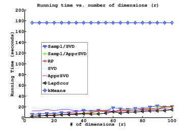
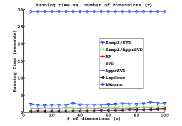
Refer to caption
(a) PIE - Running time
Refer to caption
(b) ORL - Running time
Refer to caption
(c) PIE - Objective
Refer to caption
(d) ORL - Objective
Refer to caption
(e) PIE - Accuracy of clustering
Refer to caption
(f) ORL - Accuracy of clustering
Figure 3: Plot of running time (a),(b), objective value (c),(d) and accuracy versus (e),(f) the number of projected dimensions for several dimensionality reduction approaches. Left column corresponds to the PIE dataset, whereas the right column corresponds to the ORL dataset.

7.5 Results

We present the results of our experiments in Figuresย 1,2 and 3. We experimented with relative small values for the number of dimensions:

r=5,10,15,โ€ฆ,100.๐‘Ÿ51015โ€ฆ100r=5,10,15,\dots,100.

In the synthetic dataset, we observe that all dimensionality reduction methods for k๐‘˜k-means clustering are clearly more efficient compared to naive k๐‘˜k-means clustering. More importantly, the accuracy plots of Figureย 1 demonstrate that the dimensionality reduction approach is also accurate in this case even for relatively (with respect to k๐‘˜k) small values of r๐‘Ÿr, i.e., โ‰ˆ20absent20\approx 20. Recall that in this case the clusters of the dataset are well-separated between each other. Hence, these observations suggest that dimensionality reduction for k๐‘˜k-means clustering is effective when applied to well-separated data points.

The behavior of the dimensionality reduction methods for k๐‘˜k-means clustering for the real-world datasets is similar with the synthetic dataset, see Figuresย 2 andย 3. That is, as the number of projecting dimensions increases, the normalized objective value of the resulting clustering decreases. Moreover, in all cases the normalized objective value of the proposed methods converge to the objective value attained by the naive k๐‘˜k-means algorithm (as the number of dimensions increases). In all cases but the PIE and COIL20 dataset, the proposed dimensionality reduction methods have superior performance compared to Laplacian Scoresย [21] both in terms of accuracy and normalized k๐‘˜k-means objective value. In the PIE and COIL20 datasets, the Laplacian Scores approach is superior compared to all other approaches in terms of accuracy. However, notice that in these two datasets the naive k๐‘˜k-means algorimhm performs poorly in terms of accuracy which indicates that the data might not be well-separated.

Regarding the running times of the algorithms notice that in some cases the running time does not necessarily increased by increasing the number of dimensions. This happens because after the dimensionality reduction step the k๐‘˜k-means method might take a different number of iterations to converge. We did not investigated this behavior further since this is not the focus of our experimental evaluation.

Our experiments indicate that running our algorithms with small values of r๐‘Ÿr, e.g., r=20๐‘Ÿ20r=20 or r=30๐‘Ÿ30r=30, achieves nearly optimal separation of a mixture of Gaussians and does well in several real-world clustering problems. Although a more thorough experimental evaluation of our algorithms would have been far more informative, our preliminary experimental findings are quite encouraging with respect to the performance of our algorithms in practice.

8 Conclusions

We studied the problem of dimensionality reduction for k๐‘˜k-means clustering. Most of the existing results in this topic consist of heuristic approaches, whose excellent empirical performance can not be explained with a rigorous theoretical analysis. In this paper, our focus was on dimensionality reduction methods that work well in theory. We presented three such approaches, one feature selection method for k๐‘˜k-means and two feature extraction methods. The theoretical analysis of the proposed methods is based on the fact that dimensionality reduction for k๐‘˜k-means has deep connections with low-rank approximations to the data matrix that contains the points one wants to cluster. We explained those connections in the text and employed modern fast algorithms to compute such low rank approximations and designed fast algorithms for dimensionality reduction in k๐‘˜k-means.

Despite our focus on the theoretical foundations of the proposed algorithms, we tested the proposed methods in practice and concluded that the experimental results are very encouraging: dimensionality reduction for k๐‘˜k-means using the proposed techniques leads to faster algorithms that are almost as accurate as running k๐‘˜k-means on the high dimensional data.

All in all, our work describes the first provably efficient feature selection algorithm for k๐‘˜k-means clustering as well as two novel provably efficient feature extraction algorithms. An interesting path for future research is to design provably efficient (1+ฮต)1๐œ€(1+\varepsilon)-relative error dimensionality reduction methods for k๐‘˜k-means.

References

  • [1] Feature ranking using laplacianscore. http://www.cad.zju.edu.cn/home/dengcai/Data/MCFS.html. Accessed on June 4th, 2013.
  • [2] The orl database of faces. http://www.cl.cam.ac.uk/research/dtg/attarchive/facedatabase.html. AT&T Laborartories Cambridge, UK.
  • [3] Pie database. http://www.ri.cmu.edu/research_project_detail.html?project_id=418&menu_id=261. Carnegie Mellon University.
  • [4] D.ย Achlioptas. Database-friendly random projections: Johnson-lindenstrauss with binary coins. Journal of Computer and System Sciences, 66(4):671โ€“687, 2003.
  • [5] N.ย Ailon and B.ย Chazelle. Approximate nearest neighbors and the fast johnson-lindenstrauss transform. In Proceedings of the 38th Annual ACM Symposium on Theory of Computing (STOC), 2006.
  • [6] S.ย Arora, E.ย Hazan, and S.ย Kale. A fast random sampling algorithm for sparsifying matrices. In Approximation, Randomization, and Combinatorial Optimization. Algorithms and Techniques, volume 4110 of Lecture Notes in Computer Science, pages 272โ€“279. Springer Berlin Heidelberg, 2006.
  • [7] D.ย Arthur and S.ย Vassilvitskii. k-means++: the advantages of careful seeding. In Proceedings of the eighteenth Annual ACM-SIAM Symposium on Discrete algorithms (SODA), 2007.
  • [8] K.ย Bache and M.ย Lichman. UCI machine learning repository. http://archive.ics.uci.edu/ml, 2013. University of California, Irvine, School of Information and Computer Sciences.
  • [9] C.ย Boutsidis, P.ย Drineas, and M.ย Magdon-Ismail. Near optimal column based matrix reconstruction. ArXiV:1103.0995, 2011.
  • [10] C.ย Boutsidis, M.ย Mahoney, and P.ย Drineas. Unsupervised feature selection for the k๐‘˜k-means clustering problem. In Neural Information Processing Systems (NIPS), 2009.
  • [11] K.ย L. Clarkson. Tighter bounds for random projections of manifolds. In Proceedings of the 24th Annual Symposium on Computational Geometry (SoCG), 2008.
  • [12] P.ย Drineas, A.ย Frieze, R.ย Kannan, S.ย Vempala, and V.ย Vinay. Clustering in large graphs and matrices. In Proceedings of the 10th Annual ACM-SIAM Symposium on Discrete Algorithms (SODA), 1999.
  • [13] P.ย Drineas, R.ย Kannan, and M.ย Mahoney. Fast Monte Carlo algorithms for matrices I: Approximating matrix multiplication. SIAM Journal of Computing, 36(1):132โ€“157, 2006.
  • [14] D.ย Feldman, M.ย Schmidt, and C.ย Sohler. Turning big data into tiny data: Constant-size coresets for k-means, pca and projective clustering. In SODA, pages 1434โ€“1453. SIAM, 2013.
  • [15] G.ย Frahling and C.ย Sohler. A fast k-means implementation using coresets. In Proceedings of the 22nd Annual Symposium on Computational Geometry (SoCG), 2006.
  • [16] I.ย Guyon and A.ย Elisseeff. An introduction to variable and feature selection. Journal of Machince Learning Research, 3:1157โ€“1182, 2003.
  • [17] I.ย Guyon, S.ย Gunn, A.ย Ben-Hur, and G.ย Dror. Result Analysis of the NIPS 2003 Feature Selection Challenge. In Neural Information Processing Systems (NIPS), 2005.
  • [18] S.ย Har-Peled and A.ย Kushal. Smaller coresets for k๐‘˜k-median and k๐‘˜k-means clustering. In Proceedings of the 21st Annual Symposium on Computational Geometry (SoCG), 2005.
  • [19] S.ย Har-Peled and S.ย Mazumdar. On coresets for k-means and k-median clustering. In Proceedings of the 36th Annual ACM Symposium on Theory of Computing (STOC), 2004.
  • [20] J.ย Hartigan. Clustering algorithms. John Wiley & Sons, 1975.
  • [21] X.ย He, D.ย Cai, and P.ย Niyogi. Laplacian Score for Feature Selection. In Y.ย Weiss, B.ย Schรถlkopf, and J.ย Platt, editors, Neural Information Processing Systems (NIPS), pages 507โ€“514. 2006.
  • [22] P.ย Indyk and R.ย Motwani. Approximate nearest neighbors: towards removing the curse of dimensionality. In Proceedings of the 30th Annual ACM Symposium on Theory of computing (STOC), 1998.
  • [23] W.ย Johnson and J.ย Lindenstrauss. Extensions of Lipschitz mappings into a Hilbert space. Contemporary mathematics, 26:189โ€“206, 1984.
  • [24] A.ย Kumar, Y.ย Sabharwal, and S.ย Sen. A simple linear time (1+ฯต1italic-ฯต1+\epsilon)-approximation algorithm for k-means clustering in any dimensions. In Proceedings of the 45th Annual IEEE Symposium on Foundations of Computer Science (FOCS), 2004.
  • [25] E.ย Liberty and S.ย Zucker. The Mailman algorithm: A note on matrix-vector multiplication. Information Processing Letters, 109(3):179โ€“182, 2009.
  • [26] S.ย Lloyd. Least squares quantization in PCM. IEEE Transactions on Information Theory, 28(2):129โ€“137, 1982.
  • [27] M.ย Magdon-Ismail. Row sampling for matrix algorithms via a non-commutative bernstein bound. ArXiv:1008.0587, 2010.
  • [28] MATLAB. 7.13.0.564 (R2011b). The MathWorks Inc., Natick, Massachusetts, 2010.
  • [29] S.ย A. Nene, S.ย K. Nayar, and H.ย Murase. Columbia university image library. http://www.cs.columbia.edu/CAVE/software/softlib/coil-20.php. Technical Report CUCS-005-96, February 1996.
  • [30] R.ย Ostrovsky and Y.ย Rabani. Polynomial time approximation schemes for geometric k๐‘˜k-clustering. In Proceedings of the 41th Annual IEEE Symposium on Foundations of Computer Science (FOCS), 2000.
  • [31] R.ย Ostrovsky, Y.ย Rabani, L.ย J. Schulman, and C.ย Swamy. The effectiveness of lloyd-type methods for the k๐‘˜k-means problem. In Proceedings of the 47th Annual IEEE Symposium on Foundations of Computer Science (FOCS), 2006.
  • [32] M.ย Rudelson and R.ย Vershynin. Sampling from large matrices: An approach through geometric functional analysis. Journal of the ACM, 54, 2007.
  • [33] T.ย Sarlos. Improved approximation algorithms for large matrices via random projections. In Proceedings of the 47th Annual IEEE Symposium on Foundations of Computer Science (FOCS), 2006.
  • [34] M.ย D. Vose. A linear algorithm for generating random numbers with a given distribution. Software Engineering, IEEE Transactions on, 17(9):972โ€“975, 1991.
  • [35] X.ย Wu and etย al. Top 10 algorithms in data mining. Knowledge and Information Systems, 14(1):1โ€“37, 2008.

Appendix

The following technical lemma is useful in the proof of Lemmaย 8 and the proof of Lemmaย 10.

Lemma 14.

Let ๐โˆˆโ„nร—k๐superscriptโ„๐‘›๐‘˜{\mathbf{Q}}\in\R^{n\times k} with n>k๐‘›๐‘˜n>k and ๐Tโ€‹๐=๐ˆksuperscript๐T๐subscript๐ˆ๐‘˜{\mathbf{Q}}^{\textsc{T}}{\mathbf{Q}}={\mathbf{I}}_{k}. Let ๐šฏ๐šฏ{\mathbf{\Theta}} be any nร—r๐‘›๐‘Ÿn\times r matrix (r>k๐‘Ÿ๐‘˜r>k) satisfying 1โˆ’ฮตโ‰คฯƒi2โ€‹(๐Tโ€‹๐šฏ)โ‰ค1+ฮต1๐œ€subscriptsuperscript๐œŽ2๐‘–superscript๐T๐šฏ1๐œ€1-\varepsilon\leq\sigma^{2}_{i}({\mathbf{Q}}^{\textsc{T}}{\mathbf{\Theta}})\leq 1+\varepsilon for every i=1,โ€ฆ,k๐‘–1โ€ฆ๐‘˜i=1,\dots,k and 0<ฮต<1/30๐œ€130<\varepsilon<1/3. Then,

โ€‹โ€–(๐Tโ€‹๐šฏ)โ€ โˆ’(๐Tโ€‹๐šฏ)Tโ€–2โ‰คฮต1โˆ’ฮตโ‰ค1.5โ€‹ฮต.subscriptnormsuperscriptsuperscript๐T๐šฏโ€ superscriptsuperscript๐T๐šฏT2๐œ€1๐œ€1.5๐œ€\mbox{}\|({\mathbf{Q}}^{\textsc{T}}{\mathbf{\Theta}})^{\dagger}-({\mathbf{Q}}^{\textsc{T}}{\mathbf{\Theta}})^{\textsc{T}}\|_{2}\leq{\varepsilon\over\sqrt{1-\varepsilon}}\leq 1.5\varepsilon.
Proof.

Let ๐—=๐Tโ€‹๐šฏโˆˆโ„kร—r๐—superscript๐T๐šฏsuperscriptโ„๐‘˜๐‘Ÿ{\mathbf{X}}={\mathbf{Q}}^{\textsc{T}}{\mathbf{\Theta}}\in\R^{k\times r} with SVD ๐—=๐”๐—โ€‹๐šบ๐—โ€‹๐•๐—T๐—subscript๐”๐—subscript๐šบ๐—superscriptsubscript๐•๐—T{\mathbf{X}}={\mathbf{U}}_{{\mathbf{X}}}{\mathbf{\Sigma}}_{{\mathbf{X}}}{\mathbf{V}}_{\mathbf{X}}^{\textsc{T}}. Here, ๐”๐—โˆˆโ„kร—ksubscript๐”๐—superscriptโ„๐‘˜๐‘˜{\mathbf{U}}_{{\mathbf{X}}}\in\R^{k\times k}, ๐šบ๐—โˆˆโ„kร—ksubscript๐šบ๐—superscriptโ„๐‘˜๐‘˜{\mathbf{\Sigma}}_{{\mathbf{X}}}\in\R^{k\times k}, and ๐•๐—โˆˆโ„rร—ksubscript๐•๐—superscriptโ„๐‘Ÿ๐‘˜{\mathbf{V}}_{\mathbf{X}}\in\R^{r\times k}, since r>k๐‘Ÿ๐‘˜r>k. Consider taking the SVD of (๐Tโ€‹๐šฏ)โ€ superscriptsuperscript๐T๐šฏโ€ ({\mathbf{Q}}^{\textsc{T}}{\mathbf{\Theta}})^{\dagger} and (๐Tโ€‹๐šฏ)Tsuperscriptsuperscript๐T๐šฏT({\mathbf{Q}}^{\textsc{T}}{\mathbf{\Theta}})^{\textsc{T}},

โ€‹โ€–(๐Tโ€‹๐šฏ)โ€ โˆ’(๐Tโ€‹๐šฏ)Tโ€–2=โ€‹โ€–๐•๐—โ€‹๐šบ๐—โˆ’1โ€‹๐”๐—Tโˆ’๐•๐—โ€‹๐šบ๐—โ€‹๐”๐—Tโ€–2=โ€‹โ€–๐•๐—โ€‹(๐šบ๐—โˆ’1โˆ’๐šบ๐—)โ€‹๐”๐—Tโ€–2=โ€‹โ€–๐šบ๐—โˆ’1โˆ’๐šบ๐—โ€–2,subscriptnormsuperscriptsuperscript๐T๐šฏโ€ superscriptsuperscript๐T๐šฏT2subscriptnormsubscript๐•๐—superscriptsubscript๐šบ๐—1superscriptsubscript๐”๐—Tsubscript๐•๐—subscript๐šบ๐—superscriptsubscript๐”๐—T2subscriptnormsubscript๐•๐—superscriptsubscript๐šบ๐—1subscript๐šบ๐—superscriptsubscript๐”๐—T2subscriptnormsuperscriptsubscript๐šบ๐—1subscript๐šบ๐—2\mbox{}\|({\mathbf{Q}}^{\textsc{T}}{\mathbf{\Theta}})^{\dagger}-({\mathbf{Q}}^{\textsc{T}}{\mathbf{\Theta}})^{\textsc{T}}\|_{2}=\mbox{}\|{\mathbf{V}}_{{\mathbf{X}}}{\mathbf{\Sigma}}_{{\mathbf{X}}}^{-1}{\mathbf{U}}_{{\mathbf{X}}}^{\textsc{T}}-{\mathbf{V}}_{{\mathbf{X}}}{\mathbf{\Sigma}}_{{\mathbf{X}}}{\mathbf{U}}_{{\mathbf{X}}}^{\textsc{T}}\|_{2}=\mbox{}\|{\mathbf{V}}_{{\mathbf{X}}}({\mathbf{\Sigma}}_{{\mathbf{X}}}^{-1}-{\mathbf{\Sigma}}_{{\mathbf{X}}}){\mathbf{U}}_{{\mathbf{X}}}^{\textsc{T}}\|_{2}=\mbox{}\|{\mathbf{\Sigma}}_{{\mathbf{X}}}^{-1}-{\mathbf{\Sigma}}_{{\mathbf{X}}}\|_{2},

since ๐•๐—subscript๐•๐—{\mathbf{V}}_{{\mathbf{X}}} and ๐”๐—Tsuperscriptsubscript๐”๐—T{\mathbf{U}}_{{\mathbf{X}}}^{\textsc{T}} can be dropped without changing the spectral norm. Let ๐˜=๐šบ๐—โˆ’1โˆ’๐šบ๐—โˆˆโ„kร—k๐˜superscriptsubscript๐šบ๐—1subscript๐šบ๐—superscriptโ„๐‘˜๐‘˜{\mathbf{Y}}={\mathbf{\Sigma}}_{{\mathbf{X}}}^{-1}-{\mathbf{\Sigma}}_{{\mathbf{X}}}\in\R^{k\times k} be a diagonal matrix. Then, for all i=1,โ€ฆ,k๐‘–1โ€ฆ๐‘˜i=1,\ldots,k, ๐˜iโ€‹i=1โˆ’ฯƒi2โ€‹(๐—)ฯƒiโ€‹(๐—).subscript๐˜๐‘–๐‘–1superscriptsubscript๐œŽ๐‘–2๐—subscript๐œŽ๐‘–๐—{\mathbf{Y}}_{ii}={1-\sigma_{i}^{2}({\mathbf{X}})\over\sigma_{i}({\mathbf{X}})}. Since ๐˜๐˜{\mathbf{Y}} is diagonal,

โ€‹โ€–๐˜โ€–2=max1โ‰คiโ‰คkโก|๐˜iโ€‹i|=max1โ‰คiโ‰คkโก|1โˆ’ฯƒi2โ€‹(๐—)ฯƒiโ€‹(๐—)|=max1โ‰คiโ‰คkโก|1โˆ’ฯƒi2โ€‹(๐—)|ฯƒiโ€‹(๐—)โ‰คฮต1โˆ’ฮตโ‰ค1.5โ€‹ฮต.subscriptnorm๐˜2subscript1๐‘–๐‘˜subscript๐˜๐‘–๐‘–subscript1๐‘–๐‘˜1superscriptsubscript๐œŽ๐‘–2๐—subscript๐œŽ๐‘–๐—subscript1๐‘–๐‘˜1superscriptsubscript๐œŽ๐‘–2๐—subscript๐œŽ๐‘–๐—๐œ€1๐œ€1.5๐œ€\mbox{}\|{\mathbf{Y}}\|_{2}=\max_{1\leq i\leq k}\left|{\mathbf{Y}}_{ii}\right|=\max_{1\leq i\leq k}\left|{1-\sigma_{i}^{2}({\mathbf{X}})\over\sigma_{i}({\mathbf{X}})}\right|=\max_{1\leq i\leq k}{\left|1-\sigma_{i}^{2}({\mathbf{X}})\right|\over\sigma_{i}({\mathbf{X}})}\leq{\varepsilon\over\sqrt{1-\varepsilon}}\leq 1.5\varepsilon.

The first equality follows since the singular values are positive (from our choice of ฮต๐œ€\varepsilon and the left hand side of the bound for the singular values). The first inequality follows by the bound for the singular values of ๐—๐—{\mathbf{X}}. The last inequality follows by the assumption that 0<ฮต<1/30๐œ€130<\varepsilon<1/3. ย 

Proof of Lemma 8

Proof.

We begin with the analysis of a matrix-multiplication-type term involving the multiplication of the matrices ๐„๐„{\mathbf{E}}, ๐™๐™{\mathbf{Z}}. The sampling and rescaling matrices ๐›€,๐’๐›€๐’{\mathbf{\Omega}},{\mathbf{S}} indicate the subsampling of the columns and rows of ๐„๐„{\mathbf{E}}, ๐™๐™{\mathbf{Z}}, respectively. Eqn.ย (4) of Lemma 4 of [13] gives a bound for such ๐›€,๐’๐›€๐’{\mathbf{\Omega}},{\mathbf{S}} constructed with randomized sampling with replacement and any set of probabilities p1,p2,โ€ฆ,pnsubscript๐‘1subscript๐‘2โ€ฆsubscript๐‘๐‘›p_{1},p_{2},\dots,p_{n} (over the columns of ๐„๐„{\mathbf{E}} - rows of ๐™๐™{\mathbf{Z}}),

๐”ผโกโ€‹โ€–๐„๐™โˆ’๐„โ€‹๐›€โ€‹๐’๐’Tโ€‹๐›€Tโ€‹๐™โ€–F2โ‰คโˆ‘i=1nโ€‹โ€–๐„(i)โ€–22โ€‹โ€‹โ€–๐™(i)โ€–22rโ€‹piโˆ’1rโ€‹โ€‹โ€–๐„๐™โ€–F2.๐”ผsuperscriptsubscriptnorm๐„๐™๐„๐›€superscript๐’๐’Tsuperscript๐›€T๐™F2superscriptsubscript๐‘–1๐‘›superscriptsubscriptnormsuperscript๐„๐‘–22superscriptsubscriptnormsubscript๐™๐‘–22๐‘Ÿsubscript๐‘๐‘–1๐‘Ÿsuperscriptsubscriptnorm๐„๐™F2\operatorname{\mathbb{E}}{\mbox{}\|{\mathbf{E}}{\mathbf{Z}}-{\mathbf{E}}{\mathbf{\Omega}}{\mathbf{S}}{\mathbf{S}}^{\textsc{T}}{\mathbf{\Omega}}^{\textsc{T}}{\mathbf{Z}}\|_{\mathrm{F}}^{2}}\leq\sum_{i=1}^{n}{\mbox{}\|{\mathbf{E}}^{(i)}\|_{2}^{2}\mbox{}\|{\mathbf{Z}}_{(i)}\|_{2}^{2}\over rp_{i}}-{1\over r}\mbox{}\|{\mathbf{E}}{\mathbf{Z}}\|_{\mathrm{F}}^{2}.

Notice that ๐„๐™=๐ŸŽmร—k๐„๐™subscript0๐‘š๐‘˜{\mathbf{E}}{\mathbf{Z}}=\bm{0}_{m\times k}, by construction (see Lemmaย 4). Now, for every i=1,โ€ฆ,n๐‘–1โ€ฆ๐‘›i=1,\dots,n replace the values pi=โ€‹โ€–๐™(i)โ€–22ksubscript๐‘๐‘–superscriptsubscriptnormsubscript๐™๐‘–22๐‘˜p_{i}={\mbox{}\|{\mathbf{Z}}_{(i)}\|_{2}^{2}\over k} (in Definitionย 5) and rearrange,

๐”ผโกโ€‹โ€–๐„โ€‹๐›€โ€‹๐’๐’Tโ€‹๐›€Tโ€‹๐™โ€–F2โ‰คkrโ€‹โ€‹โ€–๐„โ€–F2.๐”ผsuperscriptsubscriptnorm๐„๐›€superscript๐’๐’Tsuperscript๐›€T๐™F2๐‘˜๐‘Ÿsuperscriptsubscriptnorm๐„F2\operatorname{\mathbb{E}}{\mbox{}\|{\mathbf{E}}{\mathbf{\Omega}}{\mathbf{S}}{\mathbf{S}}^{\textsc{T}}{\mathbf{\Omega}}^{\textsc{T}}{\mathbf{Z}}\|_{\mathrm{F}}^{2}}\leq{k\over r}\mbox{}\|{\mathbf{E}}\|_{\mathrm{F}}^{2}. (20)

Observe that Lemmaย 6 and our choice of r๐‘Ÿr, implies that w.p. 1โˆ’ฮด1๐›ฟ1-\delta,

1โˆ’ฮตโ‰คฯƒi2โ€‹(๐™Tโ€‹๐›€โ€‹๐’)โ‰ค1+ฮต,for allย โ€‹i=1,โ€ฆ,k.formulae-sequence1๐œ€superscriptsubscript๐œŽ๐‘–2superscript๐™T๐›€๐’1๐œ€for allย ๐‘–1โ€ฆ๐‘˜1-\varepsilon\leq\sigma_{i}^{2}({\mathbf{Z}}^{\textsc{T}}{\mathbf{\Omega}}{\mathbf{S}})\leq 1+\varepsilon,\quad\text{for all }i=1,\ldots,k. (21)

For what follows, condition on the event of Ineq.ย (21). First, ฯƒkโ€‹(๐™Tโ€‹๐›€โ€‹๐’)>0subscript๐œŽ๐‘˜superscript๐™T๐›€๐’0\sigma_{k}({\mathbf{Z}}^{\textsc{T}}{\mathbf{\Omega}}{\mathbf{S}})>0. So, rankโ€‹(๐™Tโ€‹๐›€โ€‹๐’)=kranksuperscript๐™T๐›€๐’๐‘˜\hbox{\rm rank}({\mathbf{Z}}^{\textsc{T}}{\mathbf{\Omega}}{\mathbf{S}})=k and (๐™Tโ€‹๐›€โ€‹๐’)โ€‹(๐™Tโ€‹๐›€โ€‹๐’)โ€ =๐ˆksuperscript๐™T๐›€๐’superscriptsuperscript๐™T๐›€๐’โ€ subscript๐ˆ๐‘˜({\mathbf{Z}}^{\textsc{T}}{\mathbf{\Omega}}{\mathbf{S}})({\mathbf{Z}}^{\textsc{T}}{\mathbf{\Omega}}{\mathbf{S}})^{\dagger}={\mathbf{I}}_{k}555To see this, let ๐=๐™Tโ€‹๐›€โ€‹๐’โˆˆโ„kร—r๐superscript๐™T๐›€๐’superscriptโ„๐‘˜๐‘Ÿ{\mathbf{B}}={\mathbf{Z}}^{\textsc{T}}{\mathbf{\Omega}}{\mathbf{S}}\in\R^{k\times r} with SVD ๐=๐”๐โ€‹๐šบ๐โ€‹๐•๐T๐subscript๐”๐subscript๐šบ๐superscriptsubscript๐•๐T{\mathbf{B}}={\mathbf{U}}_{{\mathbf{B}}}{\mathbf{\Sigma}}_{{\mathbf{B}}}{\mathbf{V}}_{\mathbf{B}}^{\textsc{T}}. Here, ๐”๐โˆˆโ„kร—ksubscript๐”๐superscriptโ„๐‘˜๐‘˜{\mathbf{U}}_{{\mathbf{B}}}\in\R^{k\times k}, ๐šบ๐โˆˆโ„kร—ksubscript๐šบ๐superscriptโ„๐‘˜๐‘˜{\mathbf{\Sigma}}_{{\mathbf{B}}}\in\R^{k\times k}, and ๐•๐โˆˆโ„rร—ksubscript๐•๐superscriptโ„๐‘Ÿ๐‘˜{\mathbf{V}}_{\mathbf{B}}\in\R^{r\times k}, since r>k๐‘Ÿ๐‘˜r>k. Finally, (๐™Tโ€‹๐›€โ€‹๐’)โ€‹(๐™Tโ€‹๐›€โ€‹๐’)โ€ =๐”๐โ€‹๐šบ๐โ€‹๐•๐Tโ€‹๐•๐โŸ๐ˆkโ€‹๐šบ๐โˆ’1โ€‹๐”๐T=๐”๐โ€‹๐šบ๐โ€‹๐šบ๐โˆ’1โŸ๐ˆkโ€‹๐”๐T=๐ˆksuperscript๐™T๐›€๐’superscriptsuperscript๐™T๐›€๐’โ€ subscript๐”๐subscript๐šบ๐subscriptโŸsuperscriptsubscript๐•๐Tsubscript๐•๐subscript๐ˆ๐‘˜subscriptsuperscript๐šบ1๐superscriptsubscript๐”๐Tsubscript๐”๐subscriptโŸsubscript๐šบ๐subscriptsuperscript๐šบ1๐subscript๐ˆ๐‘˜superscriptsubscript๐”๐Tsubscript๐ˆ๐‘˜({\mathbf{Z}}^{\textsc{T}}{\mathbf{\Omega}}{\mathbf{S}})({\mathbf{Z}}^{\textsc{T}}{\mathbf{\Omega}}{\mathbf{S}})^{\dagger}={\mathbf{U}}_{{\mathbf{B}}}{\mathbf{\Sigma}}_{{\mathbf{B}}}\underbrace{{\mathbf{V}}_{\mathbf{B}}^{\textsc{T}}{\mathbf{V}}_{\mathbf{B}}}_{{\mathbf{I}}_{k}}{\mathbf{\Sigma}}^{-1}_{{\mathbf{B}}}{\mathbf{U}}_{{\mathbf{B}}}^{\textsc{T}}={\mathbf{U}}_{{\mathbf{B}}}\underbrace{{\mathbf{\Sigma}}_{{\mathbf{B}}}{\mathbf{\Sigma}}^{-1}_{{\mathbf{B}}}}_{{\mathbf{I}}_{k}}{\mathbf{U}}_{{\mathbf{B}}}^{\textsc{T}}={\mathbf{I}}_{k}.. Now, ๐€๐™๐™Tโˆ’๐€๐™๐™Tโ€‹๐›€โ€‹๐’โ€‹(๐™Tโ€‹๐›€โ€‹๐’)โ€ โ€‹๐™T=๐€๐™๐™Tโˆ’๐€๐™๐ˆkโ€‹๐™T=๐ŸŽmร—n.superscript๐€๐™๐™Tsuperscript๐€๐™๐™T๐›€๐’superscriptsuperscript๐™T๐›€๐’โ€ superscript๐™Tsuperscript๐€๐™๐™Tsubscript๐€๐™๐ˆ๐‘˜superscript๐™Tsubscript0๐‘š๐‘›{\mathbf{A}}{\mathbf{Z}}{\mathbf{Z}}^{\textsc{T}}-{\mathbf{A}}{\mathbf{Z}}{\mathbf{Z}}^{\textsc{T}}{\mathbf{\Omega}}{\mathbf{S}}({\mathbf{Z}}^{\textsc{T}}{\mathbf{\Omega}}{\mathbf{S}})^{\dagger}{\mathbf{Z}}^{\textsc{T}}={\mathbf{A}}{\mathbf{Z}}{\mathbf{Z}}^{\textsc{T}}-{\mathbf{A}}{\mathbf{Z}}{\mathbf{I}}_{k}{\mathbf{Z}}^{\textsc{T}}=\bm{0}_{m\times n}. Next, we manipulate the term ฮธ=โ€‹โ€–๐€๐™๐™Tโˆ’๐€โ€‹๐›€โ€‹๐’โ€‹(๐™Tโ€‹๐›€โ€‹๐’)โ€ โ€‹๐™Tโ€–F๐œƒsubscriptnormsuperscript๐€๐™๐™T๐€๐›€๐’superscriptsuperscript๐™T๐›€๐’โ€ superscript๐™TF\theta=\mbox{}\|{\mathbf{A}}{\mathbf{Z}}{\mathbf{Z}}^{\textsc{T}}-{\mathbf{A}}{\mathbf{\Omega}}{\mathbf{S}}({\mathbf{Z}}^{\textsc{T}}{\mathbf{\Omega}}{\mathbf{S}})^{\dagger}{\mathbf{Z}}^{\textsc{T}}\|_{\mathrm{F}} as follows (recall, ๐€=๐€๐™๐™T+๐„๐€superscript๐€๐™๐™T๐„{\mathbf{A}}={\mathbf{A}}{\mathbf{Z}}{\mathbf{Z}}^{\textsc{T}}+{\mathbf{E}}),

ฮธ=โ€‹โ€–๐€๐™๐™Tโˆ’๐€๐™๐™Tโ€‹๐›€โ€‹๐’โ€‹(๐™Tโ€‹๐›€โ€‹๐’)โ€ โ€‹๐™TโŸ๐ŸŽmร—nโˆ’๐„โ€‹๐›€โ€‹๐’โ€‹(๐™Tโ€‹๐›€โ€‹๐’)โ€ โ€‹๐™Tโ€–F=โ€‹โ€–๐„โ€‹๐›€โ€‹๐’โ€‹(๐™Tโ€‹๐›€โ€‹๐’)โ€ โ€‹๐™Tโ€–F.๐œƒsubscriptnormsubscriptโŸsuperscript๐€๐™๐™Tsuperscript๐€๐™๐™T๐›€๐’superscriptsuperscript๐™T๐›€๐’โ€ superscript๐™Tsubscript0๐‘š๐‘›๐„๐›€๐’superscriptsuperscript๐™T๐›€๐’โ€ superscript๐™TFsubscriptnorm๐„๐›€๐’superscriptsuperscript๐™T๐›€๐’โ€ superscript๐™TF\displaystyle\theta=\mbox{}\|\underbrace{{\mathbf{A}}{\mathbf{Z}}{\mathbf{Z}}^{\textsc{T}}-{\mathbf{A}}{\mathbf{Z}}{\mathbf{Z}}^{\textsc{T}}{\mathbf{\Omega}}{\mathbf{S}}({\mathbf{Z}}^{\textsc{T}}{\mathbf{\Omega}}{\mathbf{S}})^{\dagger}{\mathbf{Z}}^{\textsc{T}}}_{\bm{0}_{m\times n}}-{\mathbf{E}}{\mathbf{\Omega}}{\mathbf{S}}({\mathbf{Z}}^{\textsc{T}}{\mathbf{\Omega}}{\mathbf{S}})^{\dagger}{\mathbf{Z}}^{\textsc{T}}\|_{\mathrm{F}}=\mbox{}\|{\mathbf{E}}{\mathbf{\Omega}}{\mathbf{S}}({\mathbf{Z}}^{\textsc{T}}{\mathbf{\Omega}}{\mathbf{S}})^{\dagger}{\mathbf{Z}}^{\textsc{T}}\|_{\mathrm{F}}.

Finally, we manipulate the latter term as follows,

โ€‹โ€–๐„โ€‹๐›€โ€‹๐’โ€‹(๐™Tโ€‹๐›€โ€‹๐’)โ€ โ€‹๐™Tโ€–Fsubscriptnorm๐„๐›€๐’superscriptsuperscript๐™T๐›€๐’โ€ superscript๐™TF\displaystyle\mbox{}\|{\mathbf{E}}{\mathbf{\Omega}}{\mathbf{S}}({\mathbf{Z}}^{\textsc{T}}{\mathbf{\Omega}}{\mathbf{S}})^{\dagger}{\mathbf{Z}}^{\textsc{T}}\|_{\mathrm{F}} โ‰ค\displaystyle\leq โ€‹โ€–๐„โ€‹๐›€โ€‹๐’โ€‹(๐™Tโ€‹๐›€โ€‹๐’)โ€ โ€–Fsubscriptnorm๐„๐›€๐’superscriptsuperscript๐™T๐›€๐’โ€ F\displaystyle\mbox{}\|{\mathbf{E}}{\mathbf{\Omega}}{\mathbf{S}}({\mathbf{Z}}^{\textsc{T}}{\mathbf{\Omega}}{\mathbf{S}})^{\dagger}\|_{\mathrm{F}}
โ‰ค\displaystyle\leq โ€‹โ€–๐„โ€‹๐›€โ€‹๐’โ€‹(๐™Tโ€‹๐›€โ€‹๐’)Tโ€–F+โ€‹โ€–๐„โ€‹๐›€โ€‹๐’โ€–Fโ€‹โ€‹โ€–(๐™Tโ€‹๐›€โ€‹๐’)โ€ โˆ’(๐™Tโ€‹๐›€โ€‹๐’)Tโ€–2subscriptnorm๐„๐›€๐’superscriptsuperscript๐™T๐›€๐’TFsubscriptnorm๐„๐›€๐’Fsubscriptnormsuperscriptsuperscript๐™T๐›€๐’โ€ superscriptsuperscript๐™T๐›€๐’T2\displaystyle\mbox{}\|{\mathbf{E}}{\mathbf{\Omega}}{\mathbf{S}}({\mathbf{Z}}^{\textsc{T}}{\mathbf{\Omega}}{\mathbf{S}})^{\textsc{T}}\|_{\mathrm{F}}+\mbox{}\|{\mathbf{E}}{\mathbf{\Omega}}{\mathbf{S}}\|_{\mathrm{F}}\mbox{}\|({\mathbf{Z}}^{\textsc{T}}{\mathbf{\Omega}}{\mathbf{S}})^{\dagger}-({\mathbf{Z}}^{\textsc{T}}{\mathbf{\Omega}}{\mathbf{S}})^{\textsc{T}}\|_{2}
โ‰ค\displaystyle\leq kฮดโ€‹rโ€‹โ€‹โ€–๐„โ€–F+1ฮดโ€‹โ€‹โ€–๐„โ€–Fโ€‹ฮต1โˆ’ฮตโ‰ค(kฮดโ€‹r+ฮตฮดโ€‹1โˆ’ฮต)โ€‹โ€‹โ€–๐„โ€–F๐‘˜๐›ฟ๐‘Ÿsubscriptnorm๐„F1๐›ฟsubscriptnorm๐„F๐œ€1๐œ€๐‘˜๐›ฟ๐‘Ÿ๐œ€๐›ฟ1๐œ€subscriptnorm๐„F\displaystyle\sqrt{{k\over\delta r}}\mbox{}\|{\mathbf{E}}\|_{\mathrm{F}}+{1\over\sqrt{\delta}}\mbox{}\|{\mathbf{E}}\|_{\mathrm{F}}{\varepsilon\over\sqrt{1-\varepsilon}}\leq\left(\sqrt{{k\over\delta r}}+{\varepsilon\over\sqrt{\delta}\sqrt{1-\varepsilon}}\right)\mbox{}\|{\mathbf{E}}\|_{\mathrm{F}}
โ‰ค\displaystyle\leq (ฮต2โ€‹ฮดโ€‹1lnโก(2โ€‹k/ฮด)+ฮตฮดโ€‹1โˆ’ฮต)โ€‹โ€‹โ€–๐„โ€–F๐œ€2๐›ฟ12๐‘˜๐›ฟ๐œ€๐›ฟ1๐œ€subscriptnorm๐„F\displaystyle\left({\varepsilon\over 2\sqrt{\delta}}{1\over\sqrt{\ln(2k/\delta)}}+{\varepsilon\over\sqrt{\delta}\sqrt{1-\varepsilon}}\right)\mbox{}\|{\mathbf{E}}\|_{\mathrm{F}}
โ‰ค\displaystyle\leq (ฮต2โ€‹lnโก(4)โ€‹ฮด+ฮตฮดโ€‹1โˆ’ฮต)โ€‹โ€‹โ€–๐„โ€–Fโ‰ค1.6โ€‹ฮตฮดโ€‹โ€‹โ€–๐„โ€–F.๐œ€24๐›ฟ๐œ€๐›ฟ1๐œ€subscriptnorm๐„F1.6๐œ€๐›ฟsubscriptnorm๐„F\displaystyle\left({\varepsilon\over 2\ln(4)\sqrt{\delta}}+{\varepsilon\over\sqrt{\delta}\sqrt{1-\varepsilon}}\right)\mbox{}\|{\mathbf{E}}\|_{\mathrm{F}}\leq{1.6\varepsilon\over\sqrt{\delta}}\mbox{}\|{\mathbf{E}}\|_{\mathrm{F}}.

The first inequality follows by spectral submultiplicativity and the fact that โ€‹โ€–๐™Tโ€–2=1subscriptnormsuperscript๐™T21\mbox{}\|{\mathbf{Z}}^{\textsc{T}}\|_{2}=1. The second inequality follows by the triangle inequality for matrix norms. In the third inequality, the bound for the term โ€‹โ€–๐„โ€‹๐›€โ€‹๐’โ€‹(๐™Tโ€‹๐›€โ€‹๐’)Tโ€–Fsubscriptnorm๐„๐›€๐’superscriptsuperscript๐™T๐›€๐’TF\mbox{}\|{\mathbf{E}}{\mathbf{\Omega}}{\mathbf{S}}({\mathbf{Z}}^{\textsc{T}}{\mathbf{\Omega}}{\mathbf{S}})^{\textsc{T}}\|_{\mathrm{F}} follows by applying to it Markovโ€™s inequality together with Ineq.ย (20); also, โ€‹โ€–๐„โ€‹๐›€โ€‹๐’โ€–Fsubscriptnorm๐„๐›€๐’F\mbox{}\|{\mathbf{E}}{\mathbf{\Omega}}{\mathbf{S}}\|_{\mathrm{F}} is bounded by (1/ฮด)โ€‹โ€‹โ€–๐„โ€–F1๐›ฟsubscriptnorm๐„F(1/\sqrt{\delta})\mbox{}\|{\mathbf{E}}\|_{\mathrm{F}} w.p. 1โˆ’ฮด1๐›ฟ1-\delta (Lemmaย 7), while we bound โ€‹โ€–(๐™Tโ€‹๐›€โ€‹๐’)โ€ โˆ’(๐™Tโ€‹๐›€โ€‹๐’)Tโ€–2subscriptnormsuperscriptsuperscript๐™T๐›€๐’โ€ superscriptsuperscript๐™T๐›€๐’T2\mbox{}\|({\mathbf{Z}}^{\textsc{T}}{\mathbf{\Omega}}{\mathbf{S}})^{\dagger}-({\mathbf{Z}}^{\textsc{T}}{\mathbf{\Omega}}{\mathbf{S}})^{\textsc{T}}\|_{2} using Lemmaย 14 (set ๐=๐™๐๐™{\mathbf{Q}}={\mathbf{Z}} and ๐šฏ=๐›€โ€‹๐’๐šฏ๐›€๐’{\mathbf{\Theta}}={\mathbf{\Omega}}{\mathbf{S}} ). So, by the union bound, the failure probability is 3โ€‹ฮด3๐›ฟ3\delta. The rest of the argument follows by our choice of r๐‘Ÿr, assuming kโ‰ฅ2๐‘˜2k\geq 2, ฮต<1/3๐œ€13\varepsilon<1/3 and simple algebraic manipulations. ย 

Proof of Lemmaย 9

Proof.

First, define the random variable Y=โ€‹โ€–๐˜๐‘โ€–F2๐‘Œsuperscriptsubscriptnorm๐˜๐‘F2Y=\mbox{}\|{\mathbf{Y}}{\mathbf{R}}\|_{\mathrm{F}}^{2}. It is easy to see that ๐”ผโกY=โ€‹โ€–๐˜โ€–F2๐”ผ๐‘Œsuperscriptsubscriptnorm๐˜F2\operatorname{\mathbb{E}}{Y}=\mbox{}\|{\mathbf{Y}}\|_{\mathrm{F}}^{2} and moreover an upper bound for the variance of Y๐‘ŒY is available in Lemmaย 888 of [33]: Varโ€‹[Y]โ‰ค2โ€‹โ€‹โ€–๐˜โ€–F4/rVardelimited-[]๐‘Œ2superscriptsubscriptnorm๐˜F4๐‘Ÿ\text{Var}\left[Y\right]\leq 2\mbox{}\|{\mathbf{Y}}\|_{\mathrm{F}}^{4}/r 666[33] assumes that the matrix ๐‘๐‘{\mathbf{R}} has i.i.d rows, each one containing four-wise independent zero-mean {1/r,โˆ’1/r}1๐‘Ÿ1๐‘Ÿ\{1/\sqrt{r},-1/\sqrt{r}\} entries. The claim in our lemma follows because our rescaled sign matrix ๐‘๐‘{\mathbf{R}} satisfies the four-wise independence assumption, by construction. . Now, Chebyshevโ€™s inequality tells us that,

โ„™(|Yโˆ’๐”ผโกY|โ‰ฅฮตโ€‹โ€‹โ€–๐˜โ€–F2)โ‰คVarโ€‹[Y]ฮต2โ€‹โ€‹โ€–๐˜โ€–F4โ‰ค2โ€‹โ€‹โ€–๐˜โ€–F4rโ€‹ฮต2โ€‹โ€‹โ€–๐˜โ€–F4โ‰ค2c0โ€‹kโ‰ค0.01.โ„™๐‘Œ๐”ผ๐‘Œ๐œ€superscriptsubscriptnorm๐˜F2Vardelimited-[]๐‘Œsuperscript๐œ€2superscriptsubscriptnorm๐˜F42superscriptsubscriptnorm๐˜F4๐‘Ÿsuperscript๐œ€2superscriptsubscriptnorm๐˜F42subscript๐‘0๐‘˜0.01\displaystyle\Prob(|Y-\operatorname{\mathbb{E}}{Y}|\geq\varepsilon\mbox{}\|{\mathbf{Y}}\|_{\mathrm{F}}^{2})\leq{\text{Var}\left[Y\right]\over\varepsilon^{2}\mbox{}\|{\mathbf{Y}}\|_{\mathrm{F}}^{4}}\leq{2\mbox{}\|{\mathbf{Y}}\|_{\mathrm{F}}^{4}\over r\varepsilon^{2}\mbox{}\|{\mathbf{Y}}\|_{\mathrm{F}}^{4}}\leq{2\over c_{0}k}\leq 0.01.

The last inequality follows by assuming c0โ‰ฅ100subscript๐‘0100c_{0}\geq 100 and the fact that k>1๐‘˜1k>1. Finally, taking square root on both sides concludes the proof. ย 

Proof of Lemma 10.

We start with the definition of the Johnson-Lindenstrauss transform.

Definition 15 (Johnson-Lindenstrauss Transform).

A random matrix ๐‘โˆˆโ„nร—r๐‘superscriptโ„๐‘›๐‘Ÿ{\mathbf{R}}\in\R^{n\times r} forms a Johnson-Lindenstrauss transform if, for any (row) vector ๐ฑโˆˆโ„n๐ฑsuperscriptโ„๐‘›\bm{x}\in\R^{n},

โ„™((1โˆ’ฮต)โ€‹โ€‹โ€–๐’™โ€–22โ‰คโ€‹โ€–๐’™โ€‹๐‘โ€–22โ‰ค(1+ฮต)โ€‹โ€‹โ€–๐’™โ€–22)โ‰ฅ1โˆ’eโˆ’Cโ€‹ฮต2โ€‹rโ„™1๐œ€superscriptsubscriptnorm๐’™22superscriptsubscriptnorm๐’™๐‘221๐œ€superscriptsubscriptnorm๐’™221superscript๐‘’๐ถsuperscript๐œ€2๐‘Ÿ\Prob{\left(\left(1-\varepsilon\right)\mbox{}\|\bm{x}\|_{2}^{2}\leq\mbox{}\|\bm{x}{\mathbf{R}}\|_{2}^{2}\leq\left(1+\varepsilon\right)\mbox{}\|\bm{x}\|_{2}^{2}\right)}\geq 1-e^{-C\varepsilon^{2}r}

where C>0๐ถ0C>0 is an absolute constant.

Notice that in order to achieve failure probability at most ฮด๐›ฟ\delta, it suffices to take r=Oโ€‹(logโก(1/ฮด)/ฮต2)๐‘Ÿ๐‘‚1๐›ฟsuperscript๐œ€2r=O(\log(1/\delta)/\varepsilon^{2}). We continue with Theorem 1.11.11.1 of [4] (properly stated to fit our notation and after minor algebraic manipulations), which indicates that a (rescaled) sign matrix ๐‘๐‘{\mathbf{R}} corresponds to a Johnson-Lindenstrauss transform as defined above.

Theorem 16 ([4]).
777This theorem is proved by first showing that a rescaled random sign matrix is a Johnson-Lindenstrauss transformย [4, Lemmaย 5.15.15.1] with constant C=36๐ถ36C=36. Then, setting an appropriate value for r๐‘Ÿr and applying the union bound over all pairs of row indices of ๐€๐€{\mathbf{A}} concludes the proof.

Let ๐€โˆˆโ„mร—n๐€superscriptโ„๐‘š๐‘›{\mathbf{A}}\in\R^{m\times n} and 0<ฮต<10๐œ€10<\varepsilon<1. Let ๐‘โˆˆโ„nร—r๐‘superscriptโ„๐‘›๐‘Ÿ{\mathbf{R}}\in\R^{n\times r} be a rescaled random sign matrix with r=36ฮต2โ€‹logโก(m)โ€‹logโก(1/ฮด)๐‘Ÿ36superscript๐œ€2๐‘š1๐›ฟr={36\over\varepsilon^{2}}\log(m)\log(1/\delta). Then for all i,j=1,โ€ฆ,mformulae-sequence๐‘–๐‘—1โ€ฆ๐‘ši,j=1,\ldots,m and w.p. at least 1โˆ’ฮด1๐›ฟ1-\delta,

(1โˆ’ฮต)โ€‹โ€‹โ€–๐€(i)โˆ’๐€(j)โ€–22โ‰คโ€‹โ€–(๐€(i)โˆ’๐€(j))โ€‹๐‘โ€–22โ‰ค(1+ฮต)โ€‹โ€‹โ€–๐€(i)โˆ’๐€(j)โ€–22.1๐œ€superscriptsubscriptnormsubscript๐€๐‘–subscript๐€๐‘—22superscriptsubscriptnormsubscript๐€๐‘–subscript๐€๐‘—๐‘221๐œ€superscriptsubscriptnormsubscript๐€๐‘–subscript๐€๐‘—22(1-\varepsilon)\mbox{}\|{\mathbf{A}}_{(i)}-{\mathbf{A}}_{(j)}\|_{2}^{2}\leq\mbox{}\|\left({\mathbf{A}}_{(i)}-{\mathbf{A}}_{(j)}\right){\mathbf{R}}\|_{2}^{2}\leq(1+\varepsilon)\mbox{}\|{\mathbf{A}}_{(i)}-{\mathbf{A}}_{(j)}\|_{2}^{2}.

In addition, we will use a matrix multiplication bound which follows from Lemmaย 666 ofย [33]. The second claim of this lemma says that for any ๐—โˆˆโ„mร—n๐—superscriptโ„๐‘š๐‘›{\mathbf{X}}\in\R^{m\times n} and ๐˜โˆˆโ„nร—p๐˜superscriptโ„๐‘›๐‘{\mathbf{Y}}\in\R^{n\times p}, if ๐‘โˆˆโ„nร—r๐‘superscriptโ„๐‘›๐‘Ÿ{\mathbf{R}}\in\R^{n\times r} is a matrix with i.i.d rows, each one containing four-wise independent zero-mean {1/r,โˆ’1/r}1๐‘Ÿ1๐‘Ÿ\{1/\sqrt{r},-1/\sqrt{r}\} entries, then,

๐”ผโกโ€‹โ€–๐—๐˜โˆ’๐—๐‘๐‘Tโ€‹๐˜โ€–F2โ‰ค2rโ€‹โ€‹โ€–๐—โ€–F2โ€‹โ€‹โ€–๐˜โ€–F2.๐”ผsuperscriptsubscriptnorm๐—๐˜superscript๐—๐‘๐‘T๐˜F22๐‘Ÿsuperscriptsubscriptnorm๐—F2superscriptsubscriptnorm๐˜F2\operatorname{\mathbb{E}}{\mbox{}\|{\mathbf{X}}{\mathbf{Y}}-{\mathbf{X}}{\mathbf{R}}{\mathbf{R}}^{\textsc{T}}{\mathbf{Y}}\|_{\mathrm{F}}^{2}}\leq{2\over r}\mbox{}\|{\mathbf{X}}\|_{\mathrm{F}}^{2}\mbox{}\|{\mathbf{Y}}\|_{\mathrm{F}}^{2}. (22)

Our random matrix ๐‘๐‘{\mathbf{R}} uses full independence, hence the above bound holds by dropping the limited independence condition.

Statement 111.

The first statement in our lemma has been proved in Corollary 111111 ofย [33], see alsoย [11, Theoremย 1.31.31.3] for a restatement. More precisely, repeat the proof of Corollary 111111 ofย [33] paying attention to the constants. That is, set ๐‚=๐•kTโ€‹๐‘Tโ€‹๐‘๐•kโˆ’๐ˆk๐‚superscriptsubscript๐•๐‘˜Tsuperscript๐‘Tsubscript๐‘๐•๐‘˜subscript๐ˆ๐‘˜{\mathbf{C}}={\mathbf{V}}_{k}^{\textsc{T}}{\mathbf{R}}^{\textsc{T}}{\mathbf{R}}{\mathbf{V}}_{k}-{\mathbf{I}}_{k} and ฮต0=1/2subscript๐œ€012\varepsilon_{0}=1/2 in Lemmaย 101010 ofย [33], and apply our JL transform with (rescaled) accuracy ฮต/4๐œ€4\varepsilon/4 on each vector of the set Tโ€ฒ:={๐•kTโ€‹๐’™|๐’™โˆˆT}assignsuperscript๐‘‡โ€ฒconditional-setsuperscriptsubscript๐•๐‘˜T๐’™๐’™๐‘‡T^{\prime}:=\{{\mathbf{V}}_{k}^{\textsc{T}}\bm{x}\ |\ \bm{x}\in T\} (which is of size at most โ‰คekโ€‹lnโก(18)absentsuperscript๐‘’๐‘˜18\leq e^{k\ln(18)}, see [6, Lemmaย 4] for this bound). So,

โ„™(โˆ€i=1,โ€ฆ,k: 1โˆ’ฮตโ‰คฯƒi2(๐•kT๐‘)โ‰ค1+ฮต)โ‰ฅ1โˆ’ekโ€‹lnโก(18)eโˆ’ฮต2โ€‹r/(36โ‹…16).\Prob{\left(\forall i=1,\dots,k:\ 1-\varepsilon\leq\sigma_{i}^{2}({\mathbf{V}}_{k}^{\textsc{T}}{\mathbf{R}})\leq 1+\varepsilon\right)}\geq 1-e^{k\ln(18)}e^{-\varepsilon^{2}r/(36\cdot 16)}. (23)

Setting r๐‘Ÿr such that the failure probability is at most 0.010.010.01 indicates that r๐‘Ÿr should be at least rโ‰ฅ576โ€‹(kโ€‹lnโก(18)+lnโก(100))/ฮต2๐‘Ÿ576๐‘˜18100superscript๐œ€2r\geq 576(k\ln(18)+\ln(100))/\varepsilon^{2}. So, c0=3330subscript๐‘03330c_{0}=3330 is a sufficiently large constant for the lemma.

Statement 222.

Consider the following three events (w.r.t. the randomness of the random matrix ๐‘๐‘{\mathbf{R}}): โ„ฐ1:={1โˆ’ฮตโ‰คฯƒi2โ€‹(๐•kTโ€‹๐‘)โ‰ค1+ฮต}assignsubscriptโ„ฐ11๐œ€superscriptsubscript๐œŽ๐‘–2superscriptsubscript๐•๐‘˜T๐‘1๐œ€\mathcal{E}_{1}:=\{1-\varepsilon\leq\sigma_{i}^{2}({\mathbf{V}}_{k}^{\textsc{T}}{\mathbf{R}})\leq 1+\varepsilon\}, โ„ฐ2:={โ€–๐€ฯโˆ’kโ€‹๐‘โˆฅF2โ‰ค(1+ฮต)โ€‹โ€‹โ€–๐€ฯโˆ’kโ€–F2}assignsubscriptโ„ฐ2conditional-setevaluated-atsubscript๐€๐œŒ๐‘˜๐‘F21๐œ€superscriptsubscriptnormsubscript๐€๐œŒ๐‘˜F2\mathcal{E}_{2}:=\{\mbox{}\|{\mathbf{A}}_{\rho-k}{\mathbf{R}}\|_{\mathrm{F}}^{2}\leq(1+\varepsilon)\mbox{}\|{\mathbf{A}}_{\rho-k}\|_{\mathrm{F}}^{2}\} and โ„ฐ3:={โ€–๐€ฯโˆ’kโ€‹๐‘๐‘Tโ€‹๐•kโˆฅF2โ‰คฮต2โ€‹โ€‹โ€–๐€ฯโˆ’kโ€–F2}assignsubscriptโ„ฐ3conditional-setevaluated-atsubscript๐€๐œŒ๐‘˜superscript๐‘๐‘Tsubscript๐•๐‘˜F2superscript๐œ€2superscriptsubscriptnormsubscript๐€๐œŒ๐‘˜F2\mathcal{E}_{3}:=\{\mbox{}\|{\mathbf{A}}_{\rho-k}{\mathbf{R}}{\mathbf{R}}^{\textsc{T}}{\mathbf{V}}_{k}\|_{\mathrm{F}}^{2}\leq\varepsilon^{2}\mbox{}\|{\mathbf{A}}_{\rho-k}\|_{\mathrm{F}}^{2}\}. Ineq.ย (23) and Lemmaย 9 with ๐˜=๐€ฯโˆ’k๐˜subscript๐€๐œŒ๐‘˜{\mathbf{Y}}={\mathbf{A}}_{\rho-k} imply that โ„™(โ„ฐ1)โ‰ฅ0.99โ„™subscriptโ„ฐ10.99\Prob{(\mathcal{E}_{1})}\geq 0.99, โ„™(โ„ฐ2)โ‰ฅ0.99โ„™subscriptโ„ฐ20.99\Prob{(\mathcal{E}_{2})}\geq 0.99, respectively. A crucial observation for bounding the failure probability of the last event โ„ฐ3subscriptโ„ฐ3\mathcal{E}_{3} is that ๐€ฯโˆ’kโ€‹๐•k=๐”ฯโˆ’kโ€‹๐šบฯโˆ’kโ€‹๐•ฯโˆ’kโŠคโ€‹๐•k=๐ŸŽmร—ksubscript๐€๐œŒ๐‘˜subscript๐•๐‘˜subscript๐”๐œŒ๐‘˜subscript๐šบ๐œŒ๐‘˜superscriptsubscript๐•๐œŒ๐‘˜topsubscript๐•๐‘˜subscript0๐‘š๐‘˜{\mathbf{A}}_{\rho-k}{\mathbf{V}}_{k}={\mathbf{U}}_{\rho-k}{\mathbf{\Sigma}}_{\rho-k}{\mathbf{V}}_{\rho-k}^{\top}{\mathbf{V}}_{k}=\mathbf{0}_{m\times k} by orthogonality of the columns of ๐•ksubscript๐•๐‘˜{\mathbf{V}}_{k} and ๐•ฯโˆ’ksubscript๐•๐œŒ๐‘˜{\mathbf{V}}_{\rho-k}. This event can now be bounded by applying Markovโ€™s Inequality on Ineq.ย (22) with ๐—=๐€ฯโˆ’k๐—subscript๐€๐œŒ๐‘˜{\mathbf{X}}={\mathbf{A}}_{\rho-k} and ๐˜=๐•k๐˜subscript๐•๐‘˜{\mathbf{Y}}={\mathbf{V}}_{k} and recalling that โ€‹โ€–๐•kโ€–F2=ksuperscriptsubscriptnormsubscript๐•๐‘˜F2๐‘˜\mbox{}\|{\mathbf{V}}_{k}\|_{\mathrm{F}}^{2}=k and r=c0โ€‹k/ฮต2๐‘Ÿsubscript๐‘0๐‘˜superscript๐œ€2r=c_{0}k/\varepsilon^{2}. Assuming c0โ‰ฅ200subscript๐‘0200c_{0}\geq 200, it follows that โ„™(โ„ฐ3)โ‰ฅ0.99โ„™subscriptโ„ฐ30.99\Prob{(\mathcal{E}_{3})}\geq 0.99 (hence, setting c0=3330subscript๐‘03330c_{0}=3330 is a sufficiently large constant for both statements). A union bound implies that these three events happen w.p. 0.970.970.97. For what follows, condition on these three events.

Let ๐„~=๐€kโˆ’(๐€๐‘)โ€‹(๐•kTโ€‹๐‘)โ€ โ€‹๐•kTโˆˆโ„mร—n~๐„subscript๐€๐‘˜๐€๐‘superscriptsuperscriptsubscript๐•๐‘˜T๐‘โ€ superscriptsubscript๐•๐‘˜Tsuperscriptโ„๐‘š๐‘›\widetilde{{\mathbf{E}}}={\mathbf{A}}_{k}-({\mathbf{A}}{\mathbf{R}})({\mathbf{V}}_{k}^{\textsc{T}}{\mathbf{R}})^{\dagger}{\mathbf{V}}_{k}^{\textsc{T}}\in\R^{m\times n}. By setting ๐€=๐€k+๐€ฯโˆ’k๐€subscript๐€๐‘˜subscript๐€๐œŒ๐‘˜{\mathbf{A}}={\mathbf{A}}_{k}+{\mathbf{A}}_{\rho-k} and using the triangle inequality,

โ€‹โ€–๐„~โ€–Fโ‰คโ€‹โ€–๐€kโˆ’๐€kโ€‹๐‘โ€‹(๐•kTโ€‹๐‘)โ€ โ€‹๐•kTโ€–F+โ€‹โ€–๐€ฯโˆ’kโ€‹๐‘โ€‹(๐•kTโ€‹๐‘)โ€ โ€‹๐•kTโ€–F.subscriptnorm~๐„Fsubscriptnormsubscript๐€๐‘˜subscript๐€๐‘˜๐‘superscriptsuperscriptsubscript๐•๐‘˜T๐‘โ€ superscriptsubscript๐•๐‘˜TFsubscriptnormsubscript๐€๐œŒ๐‘˜๐‘superscriptsuperscriptsubscript๐•๐‘˜T๐‘โ€ superscriptsubscript๐•๐‘˜TF\mbox{}\|\widetilde{{\mathbf{E}}}\|_{\mathrm{F}}\ \leq\ \mbox{}\|{\mathbf{A}}_{k}-{\mathbf{A}}_{k}{\mathbf{R}}({\mathbf{V}}_{k}^{\textsc{T}}{\mathbf{R}})^{\dagger}{\mathbf{V}}_{k}^{\textsc{T}}\|_{\mathrm{F}}\ +\ \mbox{}\|{\mathbf{A}}_{\rho-k}{\mathbf{R}}({\mathbf{V}}_{k}^{\textsc{T}}{\mathbf{R}})^{\dagger}{\mathbf{V}}_{k}^{\textsc{T}}\|_{\mathrm{F}}.

The event โ„ฐ1subscriptโ„ฐ1\mathcal{E}_{1} implies that rankโ€‹(๐•kTโ€‹๐‘)=kranksuperscriptsubscript๐•๐‘˜T๐‘๐‘˜\text{rank}({\mathbf{V}}_{k}^{\textsc{T}}{\mathbf{R}})=k thus888To see this, let ๐=๐•kTโ€‹๐‘โˆˆโ„kร—r๐superscriptsubscript๐•๐‘˜T๐‘superscriptโ„๐‘˜๐‘Ÿ{\mathbf{B}}={\mathbf{V}}_{k}^{\textsc{T}}{\mathbf{R}}\in\R^{k\times r} with SVD ๐=๐”๐โ€‹๐šบ๐โ€‹๐•๐T๐subscript๐”๐subscript๐šบ๐superscriptsubscript๐•๐T{\mathbf{B}}={\mathbf{U}}_{{\mathbf{B}}}{\mathbf{\Sigma}}_{{\mathbf{B}}}{\mathbf{V}}_{\mathbf{B}}^{\textsc{T}}. Here, ๐”๐โˆˆโ„kร—ksubscript๐”๐superscriptโ„๐‘˜๐‘˜{\mathbf{U}}_{{\mathbf{B}}}\in\R^{k\times k}, ๐šบ๐โˆˆโ„kร—ksubscript๐šบ๐superscriptโ„๐‘˜๐‘˜{\mathbf{\Sigma}}_{{\mathbf{B}}}\in\R^{k\times k}, and ๐•๐โˆˆโ„rร—ksubscript๐•๐superscriptโ„๐‘Ÿ๐‘˜{\mathbf{V}}_{\mathbf{B}}\in\R^{r\times k}, since r>k๐‘Ÿ๐‘˜r>k. Finally, (๐•kTโ€‹๐‘)โ€‹(๐•kTโ€‹๐‘)โ€ =๐”๐โ€‹๐šบ๐โ€‹๐•๐Tโ€‹๐•๐โŸ๐ˆkโ€‹๐šบ๐โˆ’1โ€‹๐”๐T=๐”๐โ€‹๐šบ๐โ€‹๐šบ๐โˆ’1โŸ๐ˆkโ€‹๐”๐T=๐ˆksuperscriptsubscript๐•๐‘˜T๐‘superscriptsuperscriptsubscript๐•๐‘˜T๐‘โ€ subscript๐”๐subscript๐šบ๐subscriptโŸsuperscriptsubscript๐•๐Tsubscript๐•๐subscript๐ˆ๐‘˜subscriptsuperscript๐šบ1๐superscriptsubscript๐”๐Tsubscript๐”๐subscriptโŸsubscript๐šบ๐subscriptsuperscript๐šบ1๐subscript๐ˆ๐‘˜superscriptsubscript๐”๐Tsubscript๐ˆ๐‘˜({\mathbf{V}}_{k}^{\textsc{T}}{\mathbf{R}})({\mathbf{V}}_{k}^{\textsc{T}}{\mathbf{R}})^{\dagger}={\mathbf{U}}_{{\mathbf{B}}}{\mathbf{\Sigma}}_{{\mathbf{B}}}\underbrace{{\mathbf{V}}_{\mathbf{B}}^{\textsc{T}}{\mathbf{V}}_{\mathbf{B}}}_{{\mathbf{I}}_{k}}{\mathbf{\Sigma}}^{-1}_{{\mathbf{B}}}{\mathbf{U}}_{{\mathbf{B}}}^{\textsc{T}}={\mathbf{U}}_{{\mathbf{B}}}\underbrace{{\mathbf{\Sigma}}_{{\mathbf{B}}}{\mathbf{\Sigma}}^{-1}_{{\mathbf{B}}}}_{{\mathbf{I}}_{k}}{\mathbf{U}}_{{\mathbf{B}}}^{\textsc{T}}={\mathbf{I}}_{k}.,

(๐•kTโ€‹๐‘)โ€‹(๐•kTโ€‹๐‘)โ€ =๐ˆk.superscriptsubscript๐•๐‘˜T๐‘superscriptsuperscriptsubscript๐•๐‘˜T๐‘โ€ subscript๐ˆ๐‘˜({\mathbf{V}}_{k}^{\textsc{T}}{\mathbf{R}})({\mathbf{V}}_{k}^{\textsc{T}}{\mathbf{R}})^{\dagger}={\mathbf{I}}_{k}.

Replacing ๐€k=๐”kโ€‹๐šบkโ€‹๐•kTsubscript๐€๐‘˜subscript๐”๐‘˜subscript๐šบ๐‘˜superscriptsubscript๐•๐‘˜T{\mathbf{A}}_{k}={\mathbf{U}}_{k}{\mathbf{\Sigma}}_{k}{\mathbf{V}}_{k}^{\textsc{T}} and setting (๐•kTโ€‹๐‘)โ€‹(๐•kTโ€‹๐‘)โ€ =๐ˆk,superscriptsubscript๐•๐‘˜T๐‘superscriptsuperscriptsubscript๐•๐‘˜T๐‘โ€ subscript๐ˆ๐‘˜({\mathbf{V}}_{k}^{\textsc{T}}{\mathbf{R}})({\mathbf{V}}_{k}^{\textsc{T}}{\mathbf{R}})^{\dagger}={\mathbf{I}}_{k}, we obtain that

โ€‹โ€–๐€kโˆ’๐€kโ€‹๐‘โ€‹(๐•kTโ€‹๐‘)โ€ โ€‹๐•kTโ€–F=โ€‹โ€–๐€kโˆ’๐”kโ€‹๐šบkโ€‹๐•kTโ€‹๐‘โ€‹(๐•kTโ€‹๐‘)โ€ โŸ๐ˆkโ€‹๐•kTโ€–F=โ€‹โ€–๐€kโˆ’๐”kโ€‹๐šบkโ€‹๐•kTโ€–F=0.subscriptnormsubscript๐€๐‘˜subscript๐€๐‘˜๐‘superscriptsuperscriptsubscript๐•๐‘˜T๐‘โ€ superscriptsubscript๐•๐‘˜TFsubscriptnormsubscript๐€๐‘˜subscript๐”๐‘˜subscript๐šบ๐‘˜subscriptโŸsuperscriptsubscript๐•๐‘˜T๐‘superscriptsuperscriptsubscript๐•๐‘˜T๐‘โ€ subscript๐ˆ๐‘˜superscriptsubscript๐•๐‘˜TFsubscriptnormsubscript๐€๐‘˜subscript๐”๐‘˜subscript๐šบ๐‘˜superscriptsubscript๐•๐‘˜TF0\mbox{}\|{\mathbf{A}}_{k}-{\mathbf{A}}_{k}{\mathbf{R}}({\mathbf{V}}_{k}^{\textsc{T}}{\mathbf{R}})^{\dagger}{\mathbf{V}}_{k}^{\textsc{T}}\|_{\mathrm{F}}=\mbox{}\|{\mathbf{A}}_{k}-{\mathbf{U}}_{k}{\mathbf{\Sigma}}_{k}\underbrace{{\mathbf{V}}_{k}^{\textsc{T}}{\mathbf{R}}({\mathbf{V}}_{k}^{\textsc{T}}{\mathbf{R}})^{\dagger}}_{{\mathbf{I}}_{k}}{\mathbf{V}}_{k}^{\textsc{T}}\|_{\mathrm{F}}=\mbox{}\|{\mathbf{A}}_{k}-{\mathbf{U}}_{k}{\mathbf{\Sigma}}_{k}{\mathbf{V}}_{k}^{\textsc{T}}\|_{\mathrm{F}}=0.

To bound the second term above, we drop ๐•kTsuperscriptsubscript๐•๐‘˜T{\mathbf{V}}_{k}^{\textsc{T}}, add and subtract ๐€ฯโˆ’kโ€‹๐‘โ€‹(๐•kTโ€‹๐‘)Tsubscript๐€๐œŒ๐‘˜๐‘superscriptsuperscriptsubscript๐•๐‘˜T๐‘T{\mathbf{A}}_{\rho-k}{\mathbf{R}}({\mathbf{V}}_{k}^{\textsc{T}}{\mathbf{R}})^{\textsc{T}}, and use the triangle inequality and spectral sub-multiplicativity,

โ€‹โ€–๐€ฯโˆ’kโ€‹๐‘โ€‹(๐•kTโ€‹๐‘)โ€ โ€‹๐•kTโ€–Fsubscriptnormsubscript๐€๐œŒ๐‘˜๐‘superscriptsuperscriptsubscript๐•๐‘˜T๐‘โ€ superscriptsubscript๐•๐‘˜TF\displaystyle\mbox{}\|{\mathbf{A}}_{\rho-k}{\mathbf{R}}({\mathbf{V}}_{k}^{\textsc{T}}{\mathbf{R}})^{\dagger}{\mathbf{V}}_{k}^{\textsc{T}}\|_{\mathrm{F}} โ‰ค\displaystyle\leq โ€‹โ€–๐€ฯโˆ’kโ€‹๐‘โ€‹(๐•kTโ€‹๐‘)Tโ€–F+โ€‹โ€–๐€ฯโˆ’kโ€‹๐‘โ€‹((๐•kTโ€‹๐‘)โ€ โˆ’(๐•kTโ€‹๐‘)T)โ€–Fsubscriptnormsubscript๐€๐œŒ๐‘˜๐‘superscriptsuperscriptsubscript๐•๐‘˜T๐‘TFsubscriptnormsubscript๐€๐œŒ๐‘˜๐‘superscriptsuperscriptsubscript๐•๐‘˜T๐‘โ€ superscriptsuperscriptsubscript๐•๐‘˜T๐‘TF\displaystyle\mbox{}\|{\mathbf{A}}_{\rho-k}{\mathbf{R}}({\mathbf{V}}_{k}^{\textsc{T}}{\mathbf{R}})^{\textsc{T}}\|_{\mathrm{F}}\ +\ \mbox{}\|{\mathbf{A}}_{\rho-k}{\mathbf{R}}(({\mathbf{V}}_{k}^{\textsc{T}}{\mathbf{R}})^{\dagger}-({\mathbf{V}}_{k}^{\textsc{T}}{\mathbf{R}})^{\textsc{T}})\|_{\mathrm{F}}
โ‰ค\displaystyle\leq โ€‹โ€–๐€ฯโˆ’kโ€‹๐‘๐‘Tโ€‹๐•kโ€–F+โ€‹โ€–๐€ฯโˆ’kโ€‹๐‘โ€–Fโ€‹โ€‹โ€–(๐•kTโ€‹๐‘)โ€ โˆ’(๐•kTโ€‹๐‘)Tโ€–2.subscriptnormsubscript๐€๐œŒ๐‘˜superscript๐‘๐‘Tsubscript๐•๐‘˜Fsubscriptnormsubscript๐€๐œŒ๐‘˜๐‘Fsubscriptnormsuperscriptsuperscriptsubscript๐•๐‘˜T๐‘โ€ superscriptsuperscriptsubscript๐•๐‘˜T๐‘T2\displaystyle\mbox{}\|{\mathbf{A}}_{\rho-k}{\mathbf{R}}{\mathbf{R}}^{\textsc{T}}{\mathbf{V}}_{k}\|_{\mathrm{F}}\ +\ \mbox{}\|{\mathbf{A}}_{\rho-k}{\mathbf{R}}\|_{\mathrm{F}}\mbox{}\|({\mathbf{V}}_{k}^{\textsc{T}}{\mathbf{R}})^{\dagger}-({\mathbf{V}}_{k}^{\textsc{T}}{\mathbf{R}})^{\textsc{T}}\|_{2}.

Now, we will bound each term individually. We bound the first term using โ„ฐ3subscriptโ„ฐ3\mathcal{E}_{3}. The second term can be bounded using โ„ฐ1subscriptโ„ฐ1\mathcal{E}_{1} and โ„ฐ2subscriptโ„ฐ2\mathcal{E}_{2} together with Lemmaย 14 (set ๐=๐•k๐subscript๐•๐‘˜{\mathbf{Q}}={\mathbf{V}}_{k} and ๐šฏ=๐‘๐šฏ๐‘{\mathbf{\Theta}}={\mathbf{R}}). Hence,

โ€‹โ€–๐„~โ€–Fsubscriptnorm~๐„F\displaystyle\mbox{}\|\widetilde{{\mathbf{E}}}\|_{\mathrm{F}} โ‰ค\displaystyle\leq โ€‹โ€–๐€ฯโˆ’kโ€‹๐‘๐‘Tโ€‹๐•kโ€–F+โ€‹โ€–๐€ฯโˆ’kโ€‹๐‘โ€–Fโ€‹โ€‹โ€–(๐•kTโ€‹๐‘)โ€ โˆ’(๐•kTโ€‹๐‘)Tโ€–2subscriptnormsubscript๐€๐œŒ๐‘˜superscript๐‘๐‘Tsubscript๐•๐‘˜Fsubscriptnormsubscript๐€๐œŒ๐‘˜๐‘Fsubscriptnormsuperscriptsuperscriptsubscript๐•๐‘˜T๐‘โ€ superscriptsuperscriptsubscript๐•๐‘˜T๐‘T2\displaystyle\mbox{}\|{\mathbf{A}}_{\rho-k}{\mathbf{R}}{\mathbf{R}}^{\textsc{T}}{\mathbf{V}}_{k}\|_{\mathrm{F}}+\mbox{}\|{\mathbf{A}}_{\rho-k}{\mathbf{R}}\|_{\mathrm{F}}\mbox{}\|({\mathbf{V}}_{k}^{\textsc{T}}{\mathbf{R}})^{\dagger}-({\mathbf{V}}_{k}^{\textsc{T}}{\mathbf{R}})^{\textsc{T}}\|_{2}
โ‰ค\displaystyle\leq ฮตโ€‹โ€‹โ€–๐€ฯโˆ’kโ€–F+(1+ฮต)โ€‹โ€‹โ€–๐€ฯโˆ’kโ€–Fโ‹…1.5โ€‹ฮต๐œ€subscriptnormsubscript๐€๐œŒ๐‘˜Fโ‹…1๐œ€subscriptnormsubscript๐€๐œŒ๐‘˜F1.5๐œ€\displaystyle\varepsilon\mbox{}\|{\mathbf{A}}_{\rho-k}\|_{\mathrm{F}}+\sqrt{(1+\varepsilon)}\mbox{}\|{\mathbf{A}}_{\rho-k}\|_{\mathrm{F}}\cdot 1.5\varepsilon
โ‰ค\displaystyle\leq ฮตโ€‹โ€‹โ€–๐€ฯโˆ’kโ€–F+2โ€‹ฮตโ€‹โ€‹โ€–๐€ฯโˆ’kโ€–F๐œ€subscriptnormsubscript๐€๐œŒ๐‘˜F2๐œ€subscriptnormsubscript๐€๐œŒ๐‘˜F\displaystyle\varepsilon\mbox{}\|{\mathbf{A}}_{\rho-k}\|_{\mathrm{F}}+2\varepsilon\mbox{}\|{\mathbf{A}}_{\rho-k}\|_{\mathrm{F}}
=\displaystyle= 3โ€‹ฮตโ‹…โ€‹โ€–๐€ฯโˆ’kโ€–F.โ‹…3๐œ€subscriptnormsubscript๐€๐œŒ๐‘˜F\displaystyle 3\varepsilon\cdot\mbox{}\|{\mathbf{A}}_{\rho-k}\|_{\mathrm{F}}.

The last inequality holds by our choice of ฮตโˆˆ(0,1/3)๐œ€013\varepsilon\in(0,1/3). ย 

Proof of Eqn.ย (3)

Proof.

๐”ผโกโ€‹โ€–๐„โ€–F2โ‰ค(1+ฮต)โ€‹โ€‹โ€–๐€โˆ’๐€kโ€–F2โ†’๐”ผโกโ€‹โ€–๐„โ€–F2โˆ’โ€‹โ€–๐€โˆ’๐€kโ€–F2โ‰คฮตโ€‹โ€‹โ€–๐€โˆ’๐€kโ€–F2.๐”ผsuperscriptsubscriptnorm๐„F21๐œ€superscriptsubscriptnorm๐€subscript๐€๐‘˜F2โ†’๐”ผsuperscriptsubscriptnorm๐„F2superscriptsubscriptnorm๐€subscript๐€๐‘˜F2๐œ€superscriptsubscriptnorm๐€subscript๐€๐‘˜F2\operatorname{\mathbb{E}}{\mbox{}\|{\mathbf{E}}\|_{\mathrm{F}}^{2}}\leq(1+\varepsilon)\mbox{}\|{\mathbf{A}}-{\mathbf{A}}_{k}\|_{\mathrm{F}}^{2}\rightarrow\operatorname{\mathbb{E}}{\mbox{}\|{\mathbf{E}}\|_{\mathrm{F}}^{2}-\mbox{}\|{\mathbf{A}}-{\mathbf{A}}_{k}\|_{\mathrm{F}}^{2}\leq\varepsilon\mbox{}\|{\mathbf{A}}-{\mathbf{A}}_{k}\|_{\mathrm{F}}^{2}}. Now, apply Markovโ€™s inequality on the random variable Y=โ€‹โ€–๐„โ€–F2โˆ’โ€‹โ€–๐€โˆ’๐€kโ€–F2โ‰ฅ0๐‘Œsuperscriptsubscriptnorm๐„F2superscriptsubscriptnorm๐€subscript๐€๐‘˜F20Y=\mbox{}\|{\mathbf{E}}\|_{\mathrm{F}}^{2}-\mbox{}\|{\mathbf{A}}-{\mathbf{A}}_{k}\|_{\mathrm{F}}^{2}\geq 0. (Yโ‰ฅ0๐‘Œ0Y\geq 0 because ๐„=๐€โˆ’๐€๐™๐™T๐„๐€superscript๐€๐™๐™T{\mathbf{E}}={\mathbf{A}}-{\mathbf{A}}{\mathbf{Z}}{\mathbf{Z}}^{\textsc{T}} and rankโ€‹(๐€๐™๐™T)=kranksuperscript๐€๐™๐™T๐‘˜\hbox{\rm rank}({\mathbf{A}}{\mathbf{Z}}{\mathbf{Z}}^{\textsc{T}})=k). This gives โ€‹โ€–๐„โ€–F2โˆ’โ€‹โ€–๐€โˆ’๐€kโ€–F2โ‰ค100โ€‹ฮตโ€‹โ€‹โ€–๐€โˆ’๐€kโ€–F2superscriptsubscriptnorm๐„F2superscriptsubscriptnorm๐€subscript๐€๐‘˜F2100๐œ€superscriptsubscriptnorm๐€subscript๐€๐‘˜F2\mbox{}\|{\mathbf{E}}\|_{\mathrm{F}}^{2}-\mbox{}\|{\mathbf{A}}-{\mathbf{A}}_{k}\|_{\mathrm{F}}^{2}\leq 100\varepsilon\mbox{}\|{\mathbf{A}}-{\mathbf{A}}_{k}\|_{\mathrm{F}}^{2} w.p. 0.990.990.99; so, โ€‹โ€–๐„โ€–F2โ‰คโ€‹โ€–๐€โˆ’๐€kโ€–F2+100โ€‹ฮตโ€‹โ€‹โ€–๐€โˆ’๐€kโ€–F2superscriptsubscriptnorm๐„F2superscriptsubscriptnorm๐€subscript๐€๐‘˜F2100๐œ€superscriptsubscriptnorm๐€subscript๐€๐‘˜F2\mbox{}\|{\mathbf{E}}\|_{\mathrm{F}}^{2}\leq\mbox{}\|{\mathbf{A}}-{\mathbf{A}}_{k}\|_{\mathrm{F}}^{2}+100\varepsilon\mbox{}\|{\mathbf{A}}-{\mathbf{A}}_{k}\|_{\mathrm{F}}^{2}. ย