Finite-Volume Scaling of the Wilson-Dirac Operator Spectrum

Abstract

The microscopic spectral density of the Hermitian Wilson-Dirac operator is computed numerically in quenched lattice QCD. We demonstrate that the results given for fixed index of the Wilson-Dirac operator can be matched by the predictions from Wilson chiral perturbation theory. We test successfully the finite volume and the mass scaling predicted by Wilson chiral perturbation theory at fixed lattice spacing.

I Introduction

For a long time, the Wilson construction of Dirac fermions on the lattice was somewhat overshadowed by other formulations with either explicit chiral symmetry or remnants thereof. Recently, with the help of improved simulation techniques and more powerful computers, numerical simulations with Wilson fermions have picked up momentum again. The initial concern about the explicit breaking of chiral symmetry in this formulation can be dealt with in precisely the way originally envisaged: by simply pushing simulations into the regime of very light fermions, even to the physical point of almost massless $u$ and $d$ quarks. This requires tight control on the smallest eigenvalues of the associated Wilson-Dirac operator $D_{W}$. If the lattice spacing is not small enough, the gap associated with the Hermitian Wilson-Dirac operator $D_{5}\equiv\gamma_{5}(D_{W}+m)$, where $m$ is the quark mass in continuum language, shrinks due to small eigenvalues populating the region between $-m$ and $m$. This can cause severe numerical instabilities in the simulations. Studies of the spectral gap and its potential disappearance have indicated that simulations may be continued to the physical point even at realistic lattice spacings of present-day computational power Luscher .

Sparked by this renewed interest in simulations with Wilson fermions on the lattice, also work on analytical approaches to understanding the chiral limit of these fermions has intensified. As is always the case, it is advantageous to phrase the discussion in terms of the pertinent low-energy effective field theory, Wilson chiral perturbation theory (WCPT) Sharpe . Within this framework Sharpe Sharpe1 was the first to consider the effects of finite lattice spacing, $a$, on the spectrum of the Hermitian Wilson-Dirac operator. More recently, a complete description of the microscopic details of the Wilson-Dirac operator spectrum up to and including $a^{2}$ corrections has been presented for both quenched DSV ; ADSV ; AN ; KVZ and unquenched cases ADSVNf1 ; SVdyn . Here we will test these recent predictions against quenched lattice data.

The microscopic description works, at leading order in the chiral counting rule of the finite-volume $\epsilon$-regime, at two equivalent levels: (i) a Wilson chiral random matrix theory (WRMT) and (ii) the zero-mode sector of WCPT to order $a^{2}$. Beyond leading order only the approach based on WCPT survives.

The $\gamma_{5}$-Hermiticity of the Wilson-Dirac operator,

$$D_{W}^{\dagger}=\gamma_{5}D_{W}\gamma_{5},$$ (1)

together with the explicit form of $D_{W}$ tells us that the eigenvalues of $D_{W}$ come in complex conjugate pairs Itoh , a feeble remnant of chiral symmetry. In addition, $\gamma_{5}$-Hermiticity of $D_{W}$ ensures that the Hermitian Wilson-Dirac operator,

$$D_{5}\equiv\gamma_{5}(D_{W}+m),$$ (2)

as the name suggests, is Hermitian. While the eigenvalues of $D_{W}$ can be computed by, say, the Arnoldi algorithm, it is clearly advantageous to focus instead on the Hermitian Wilson-Dirac operator $D_{5}$, for which fast algorithms exist that provide an ascending sequence of lowest eigenvalues.

Here we test the predictions for the quenched microscopic spectral density of $D_{5}$ that were presented in DSV ; ADSV against lattice data. All results of DSV ; ADSV are given for fixed index of the Wilson-Dirac operator. This index $\nu$ is defined for a given gauge field configuration by

$$\nu~{}\equiv~{}{\sum_{k}}^{\prime}{\rm sign}(\langle k|\gamma_{5}|k\rangle).$$ (3)

Here, $|k\rangle$ denotes the $k$’th eigenstate of the Wilson-Dirac operator. Only those eigenvectors which correspond to a real eigenvalue of the Wilson-Dirac operator have a nonvanishing expectation value of $\gamma_{5}$ Itoh and hence contribute to the index.

In the microscopic limit the real eigenvalues of the Wilson-Dirac operator are predicted to be located in regions with width of order $1/V$ DSV ; ADSV ; KVZ , where $V$ is the four volume, and we choose only to include the physical/leftmost of these regions in the above definition of the index. This is indicated by the prime on the sum in Eq. (3).

The predictions DSV ; ADSV for the quenched microscopic spectral density of $D_{5}$ are based on the $\epsilon$-regime of Wilson chiral perturbation theory. At leading order in the $\epsilon$-regime of WCPT three additional low energy constants, $W_{6}$, $W_{7}$ and $W_{8}$ parametrize the leading corrections due to the nonzero lattice spacing (order $a^{2}$ corrections) Sharpe . There are large-$N_{c}$ arguments ($N_{c}$ is the number of colors) to the effect that the Wilson low-energy constants $W_{6}$ and $W_{7}$ may be small Sharpe1 . For the case $W_{6}=W_{7}=0$ it was argued in DSV ; ADSV that only $W_{8}>0$ correctly describes lattice QCD with a nonnormal and $\gamma_{5}$-Hermitian Dirac operator. In agreement with this we will demonstrate here that the quenched microscopic eigenvalue density of $D_{5}$ obtained on the lattice can be matched by the prediction from WCPT with the low energy parameters $W_{6}=0$, $W_{7}=0$ and $W_{8}>0$.

We identify the effects of nonzero $W_{6}$ and $W_{7}$ in the spectrum of $D_{5}$, and conclude that they do not change the above conclusion.

Finally, we explicitly compute the real eigenvalues of $D_{W}$ and compare to the predictions.

Wilson chiral perturbation theory has also been considered in the finite-volume scaling limit where the $a^{2}$-terms can be pulled down from the action and treated as small perturbations Shindler . The analytic constraint on $W_{8}$ that we discussed above is not obvious in such a scaling limit.

Our paper is organized as follows. In the section just below, we first briefly recall those results from WCPT in the $\epsilon$-regime that are most relevant for the present lattice study. Section III gives the definition of Wilson chiral random matrix theory. In section IV we give details of the lattice simulations we have performed. We compare our lattice data to the predictions from Wilson chiral perturbation theory in section V. Section VI contains our conclusions.

II Predictions for the microscopic spectrum

Here we recall the predictions for the spectral density of $D_{5}$,

$$\rho_{5}(\lambda^{5},m;a)=\left\langle\sum_{k}\delta(\lambda^{5}_{k}-\lambda^{5})\right\rangle.$$ (4)

The eigenvalues $\lambda^{5}$, defined by

$$D_{5}\psi_{k}=\lambda^{5}_{k}\psi_{k}$$ (5)

are considered in the microscopic limit where $V\to\infty$ while

$$mV,\quad\lambda^{5}_{k}V,\quad\quad a^{2}V$$ (6)

are kept fixed.

The microscopic spectral density follows from WCPT. To ${\cal O}(a^{2})$ accuracy this effective theory was written down in Sharpe , expanding in all operators that contribute to this order in the Szymanzik scheme. To order $a^{2}$ the zeromode partition function at fixed index $\nu$ can be obtained DSV by decomposing the momentum zeromode partition function according to

$$Z_{N_{f}}(m,\theta;a)\equiv\sum_{\nu=-\infty}^{\infty}e^{i\nu\theta}Z_{N_{f}}^{\nu}(m;a).$$ (7)

In this $\epsilon$-regime, the partition function reduces to a unitary matrix integral

$$Z_{N_{f}}^{\nu}(m,z;a)=\int_{U(N_{f})}dU\ {\det}^{\nu}U~{}e^{S[U]},$$ (8)

where the action $S[U]$ for degenerate quark masses is given by

$$S = \frac{m}{2}\Sigma V{\rm Tr}(U+U^{\dagger})+\frac{z}{2}\Sigma V{\rm Tr}(U-U^{\dagger})$$ (11)

$$-a^{2}VW_{6}[{\rm Tr}\left(U+U^{\dagger}\right)]^{2}-a^{2}VW_{7}[{\rm Tr}\left(U-U^{\dagger}\right)]^{2}$$

$$-a^{2}VW_{8}{\rm Tr}(U^{2}+{U^{\dagger}}^{2}).$$

In addition to the chiral condensate, $\Sigma$, the action contains the low-energy Wilson constants $W_{6}$, $W_{7}$ and $W_{8}$ as unknown parameters . In the continuum the decomposition (7) into a sum over sectors of index $\nu$ is unambiguous LS . At nonzero lattice spacing the terms of order $a^{2}$ in the chiral Lagrangian, however, allow one to make different decompositions corresponding to different definitions of $\theta$ and $\nu$ at $a\neq 0$. As was shown in Ref. ADSV , the specific decomposition (7-11) corresponds exactly to the definition of $\nu$ given in Eq. (3). Moreover, in the microscopic limit the real modes are predicted to be in well seprated regions each width width of order $a^{2}W_{i}/\Sigma\sim 1/V$. The gauge field configurations which contribute to the individual terms in the sum (7) can thus be identified on the basis of the spectral flow Heller0 . This provides a firm foundation for choosing this particular lattice definition of the index.

To simplify our notation, we absorb the factor of $VW_{i}$ into $a_{i}^{2}$ and the factor $V\Sigma$ into $m$, $z_{k}$ and $\lambda^{5}$

$$a^{2}VW_{i}\to\hat{a}_{i}^{2}\qquad mV\Sigma\to\hat{m}$$ (12)

$$zV\Sigma\to\hat{z}\quad\,\quad \lambda^{5}V\Sigma\to\hat{\lambda}^{5}.$$ (13)

The explicit expression for the quenched microscopic spectral density can be derived following the procedure described in Ref. DOTV , now extended to the case of a source $z$ for the pseduoscalar density. In addition, much like at nonzero chemical potential SVfact ; SVbos , one must carefully take into account the convergence of the noncompact integrals. The resulting analytical formula was obtained in DSV ; ADSV :

$$\rho^{\nu}_{5}(\hat{\lambda}^{5},\hat{m};\hat{a}_{i}) = \frac{1}{\pi}{\rm Im}\ G^{\nu}(-\hat{\lambda}^{5},\hat{m};\hat{a}_{i}),$$ (14)

where

$$G^{\nu}(\hat{z},\hat{m};\hat{a}_{i})=\int_{-\infty}^{\infty}ds\int_{-\pi}^{\pi}\frac{d\theta}{2\pi}i\cos(\theta)e^{(i\theta-s)\nu}$$ (15)

$$\times\!\exp[\!-\hat{m}\sin(\theta)\!-\!i\!\hat{m}\!\sinh(s)\!+\!i\hat{z}\cos(\theta)\!-\!i\!(\hat{z}\!-\!i\epsilon)\!\cosh(s)$$

$$+4\hat{a}_{6}^{2}(-i\sin(\theta)+\sinh(s))^{2}+4\hat{a}_{7}^{2}(\cos(\theta)-\cosh(s))^{2}$$ (16)

$$+2\hat{a}_{8}^{2}(\cos(2\theta)-\cosh(2s))]$$

$$\times\big{(}-\frac{\hat{m}}{2}\sin(\theta)+i\frac{\hat{m}}{2}\sinh(s)+i\frac{\hat{z}}{2}\cos(\theta)+i\frac{\hat{z}}{2}\cosh(s)$$

$$-4(\hat{a}_{6}^{2}+\hat{a}_{7}^{2})(\sin^{2}(\theta)+\sinh^{2}(s))$$ (17)

$$+2\hat{a}_{8}^{2}(\cos(2\theta)+\cosh(2s)+e^{i\theta+s}+e^{-i\theta-s})\!+\!\frac{1}{2}\big{)}.$$ (18)

Existence of the integrals leads to the constraint $W_{8}>0$ (for $W_{6}=W_{7}=0$) as described in detail in Refs. DSV ; ADSV . The sign of $W_{8}$ is also crucial for understanding if one approaches the so-called Aoki phase of Wilson fermions Aokiclassic . A positive sign of $W_{8}$ (and $W_{6}=W_{7}=0$) indicates that the Aoki phase will appear as the gap in the spectrum of $D_{5}$ closes. The analytic predictions of WCPT for the spectral density $D_{5}$ allow us to follow in detail how the gap disappears as $m$ is taken to zero at fixed lattice spacing $a$.

III Wilson chiral random matrix theory

As we will make explicit use of it below, we give also here the corresponding expressions in the equivalent Wilson chiral random matrix theory formulation DSV ; ADSV . The idea is to introduce the most general large-$N$ matrix that has conjugation properties similar to $\gamma_{5}$-Hermiticity. Let this matrix be

$$\tilde{D}_{W}=\left(\begin{array}[]{cc}aA&iW\\ iW^{\dagger}&aB\end{array}\right),$$ (21)

where

$$A=A^{\dagger}\quad{\rm and}\quad B^{\dagger}=B$$ (22)

are $(n+\nu)\times(n+\nu)$ and $n\times n$ complex matrices, respectively, and $W$ a rectangular complex matrix of size $(n+\nu)\times n$. As in ADSV we use tildes to indicate quantities in Wilson chiral random matrix theory which are analogues of those in the field theory. We consider the limit $N=2n+\nu\to\infty$ with $\tilde{m}N$, $\tilde{z}N$ and $\tilde{a}^{2}N$ fixed.

The matrix $\tilde{D}_{W}$ is $\tilde{\gamma}_{5}$-Hermitian with respect to

$$\tilde{\gamma}_{5}={\rm diag}(1,\cdots,1,-1,\cdots,-1)~{},$$ (23)

where the first $(n+\nu)$ entries are +1, and the remaining $n$ entries are -1.

Results based on the Wilson chiral random matrix theory are expected to be universal, as in the case of the usual chiral random matrix theory ADMN . For simplicity one can therefore take the matrix elements to be distributed with Gaussian weight

$$P(A,B,W)\equiv e^{-\frac{N}{2}{\rm Tr}[A^{2}+B^{2}]-N{\rm Tr}[WW^{\dagger}]}.$$ (24)

The partition function of the Wilson chiral random matrix theory is thus defined by

$$\tilde{Z}^{\nu}_{N_{f}}=\int\!\!dAdBdW\ \!\!\!\prod_{f=1}^{N_{f}}\det(\tilde{D}_{W}+\tilde{m}_{f}+\tilde{z}_{f}\tilde{\gamma}_{5})\ P.$$ (25)

The matrix integrals are over the complex Haar measure.

In the limit $N\to\infty$ the partition function (25) coincides with that of (8) when $W_{6}=W_{7}=0$. It is straightforward to extend the Wilson chiral random matrix theory so that also double-trace terms corresponding to $W_{6}$ and $W_{7}$ are included ADSV ; JO . The correspondence between parameters of Wilson chiral random matrix theory and Wilson chiral perturbation theory is

$$N\tilde{m}=\frac{m\Sigma V}{2},\quad N\tilde{z}=\frac{z\Sigma V}{2},\quad\frac{N\tilde{a}^{2}}{2}=a^{2}W_{8}V.$$ (26)

Once this identification is made, one can equally well use the Wilson chiral random matrix theory to derive spectral distributions. This has been demonstrated explicitly in AN ; KVZ . Moreover, since no compact expressions are presently known for individual eigenvalue distributions, it is straightforward to generate such eigenvalue distributions numerically using the Gaussian integrals of Wilson chiral random matrix theory. This will be used below.

IV The lattice setup

Here we give a few details of the lattice simulations. For this initial study we work in the quenched approximation. It is advantageous to use a pure gauge action which gives configurations with a fairly unique topological charge, i.e., a pure gauge action that suppresses so-called dislocations. Experience from simulations with domain wall fermions, for which the dislocations tend to increase the residual chiral symmetry breaking at finite fifth dimensional extent $L_{s}$, suggests that the Iwasaki gauge action Iwasaki would be a good choice. This action is fairly well studied and appears to have a rather smooth continuum limit. Our lattice parameters were chosen using $r_{0}/a$ values from interpolation formulae given in Iwasaki_r0.a ; Iwasaki_r0.b and using $r_{0}=0.5$ fm to set the physical scale.

We used a mixture of heatbath and overrelaxation updates with, as advocated in Ref. Iwasaki_r0.b , $N_{or}\approx 1.5r_{0}/a$ overrelaxation sweeps for each heatbath sweep. We saved configurations separated by 100 heatbath sweeps for our measurements. We found no detectable autocorrelations in the ensembles generated. Experience indicates that for studies of the $\epsilon$-regime of chiral perturbation theory, physical lattice sizes of $L=1.5$ to 2 fm are most useful. The lattice size is large enough so that several Dirac eigenvalues are governed by the $\epsilon$-regime of CPT, but it is small enough that sufficient statistics in sectors of given, small topological charge can be obtained. Some relevant parameters of the three ensemble considered in this study are summarized in Table 1.

Ensemble	$\beta_{Iw}$	size	$r_{0}/a$	$a$ [fm]	$L$ [fm]	# cfgs
A	2.635	$16^{4}$	5.37	0.093	1.5	6500
B	2.635	$20^{4}$	5.37	0.093	1.9	3000
C	2.79	$20^{4}$	6.70	0.075	1.5	6000

Table 1: Parameters of the pure gauge configurations considered. They are generated with the Iwasaki gauge action.

IV.1 Spectral flow

In order for the match to Wilson chiral perturbation theory to be valid the assignment of index $\nu$ to a given gauge field configuration must be obtained from Eq. (3) using either a) the (small) real eigenvalues of the Wilson-Dirac operator, together with the chiralities of the corresponding eigenvectors or equivalently b) by counting the number of net crossings of zero of the eigenvalues of the Hermitian Wilson-Dirac operator as a function of the mass parameter $m_{0}$ Heller0 and weighting their contribution by the sign of the slope at the crossing. Since we did not have an implementation of the Arnoldi algorithm to compute the (complex) eigenvalues of the Wilson-Dirac operator, including the relevant real eigenvalues, we used the spectral flow strategy.

The index determined from the real eigenvalues of the Wilson-Dirac operator, or equivalently from the spectral flow, can depend on the range of the real eigenvalues considered, or equivalently, the value of $-m_{cut}$ at which the spectral flow is terminated. With $-m_{c}$ being the critical mass, at which the pion formed from Wilson quarks becomes massless, $m_{cut}$ should be sufficiently larger than $m_{c}$, but smaller than the value at which the doubler fermions become light. For our computations we use one HYP smearing of the gauge fields HYP in the construction of the Wilson-Dirac operator to help further suppress lattice artifacts. Then the choice $m_{cut}=1.0$ is safely away from both $m_{c}$ and the doubler region. With the Iwasaki gauge action and its suppression of dislocations, crossings in the neighborhood of $m_{cut}$ are rare, but they do occur occasionally. Hence a change in $m_{cut}$ would change the index on a few configurations.

Ensemble	size	$\beta_{Iw}$	$m_{0}$	$\#$ configs
				$\nu=0,1,-1$
A	$16^{4}$	2.635	$-0.216$	1246, 1088, 1045
B	$20^{4}$	2.635	$-0.216$	379, 319, 322
C	$20^{4}$	2.79	$-0.178$	1172, 990, 988
C	$20^{4}$	2.79	$-0.184$	1172, 990, 988

Table 2:

V The Spectrum of $D_{5}$: lattice simulations

In this section we compare the microscopic spectral density of $D_{5}$ as predicted by WCPT for the quenched case to the lattice simulations described above.

The values of $m$, $\lambda^{5}$ and $a$ given in the figures refer to $\hat{m}$, $\hat{\lambda}^{5}$ and $\hat{a}_{8}$. For all plots except Figure 8 we have set $\hat{a}_{6}=\hat{a}_{7}=0$.

V.1 Volume scaling

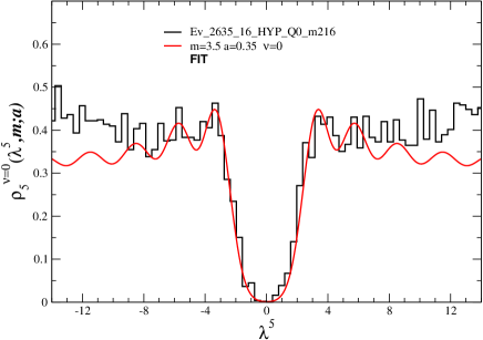
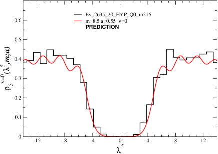
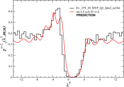
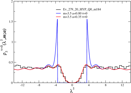
Our first test of the analytic predictions for the microscopic spectrum of $D_{5}$ concerns the finite volume scaling at fixed lattice spacing. That is, the scaling of $\hat{m}$, $\hat{\lambda}^{5}$ and $\hat{a}_{8}$ with $V$ for fixed $a$. To this end we consider the two sets of data with $\beta_{Iw}=2.635$ and $m_{0}=-0.216$, see Table 2. Because of the larger statistics obtained we first match the $16^{4}$ lattice data with $\nu=0$ to the prediction (18). The result is displayed in the top panel of Figure 1. We observe that it is possible to make a reasonable fit to the data. The range over which the predictions match the data is limited to the lowest two eigenvalues, beyond which the increasing slope of the data indicates that the $p$-regime effects set in. Given the best values found in the fit we then scale $\hat{m}$ by $20^{4}/16^{4}$ and $\hat{a}_{8}$ by $20^{2}/16^{2}$ to obtain the analytic prediction for the spectral density obtained on the $20^{4}$ lattice at the same value of the coupling and lattice mass. This parameter free prediction is plotted against the lattice data in the lower panel of Figure 1. We observe that this finite-volume scaling of the analytic prediction is consistent with the $20^{4}$ data. The limited statistics does not allow us to resolve the detailed structure of the analytic prediction.

Figure 1: The eigenvalue density of $D_{5}$ in the sector with $\nu=0$ for $V=16^{4}$ (top) and $V=20^{4}$ (bottom) both with $\beta_{Iw}=2.635$ and $m_{0}=-0.216$. The $x$-axis has been rescaled by $\Sigma V$, where $\Sigma 16^{4}=157.5$. In the top plot the smooth red curve displays a fit of the analytic prediction for the microscopic density of $D_{5}$ to the $16^{4}$ data. The fit values are $\hat{m}=3.5$ and $\hat{a}_{8}=0.35$ ($\hat{a}_{6}=\hat{a}_{7}=0$). In the plot below the smooth red line shows the prediction for the $20^{4}$ data ($\hat{m}=8.5$ and $\hat{a}_{8}=0.55$) obtained from finite volume scaling of the $16^{4}$ values. We observe that the finite volume scaling at fixed lattice spacing is well respected.

Figure 2: The eigenvalue density of $D_{5}$ in the sector with $\nu=1$ for $V=16^{4}$ (top) and $V=20^{4}$ (bottom) both with $\beta_{Iw}=2.635$ and $m_{0}=-0.216$. The $x$-axis has been rescaled by $\Sigma V$, where $\Sigma 16^{4}=157.5$. The smooth red curves displays the analytic prediction for the microscopic density of $D_{5}$. The values, $\hat{m}=3.5$ and $\hat{a}_{8}=0.35$ for $16^{4}$ and $\hat{m}=8.5$ and $\hat{a}_{8}=0.55$ are obtained from the fit in the top panel of Figure 1 and by finite volume scaling from $16^{4}$ to $20^{4}$ ($\hat{a}_{6}=\hat{a}_{7}=0$).

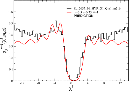
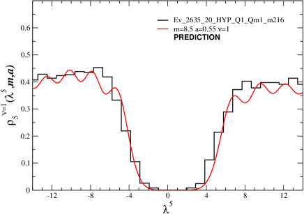
Likewise for $|\nu|=1$ we can test the analytic prediction with the parameters fixed from the fit to the $16^{4}$ and $\nu=0$ data. The result is displayed in Figure 2. Note that the analytic prediction for $-\nu$ is obtained from the one for $\nu$ by flipping the sign of $\hat{\lambda}^{5}$. To make the most of our statistics we therefore overlay the data obtained for $\nu=1$ and $\nu=-1$ flipping the sign of the eigenvalues of the latter. This is done throughout this paper. We observe that the general structure of the $16^{4}$ $\nu=1$ data is reproduced by the analytic prediction. Also the overall features of the $20^{4}$ $\nu=1$ data are followed by the parameter free analytic prediction which in this case follows from finite volume scaling.

We conclude that $W_{6}=W_{7}=0$ and $W_{8}>0$ is consistent with the lattice data at $\beta_{Iw}=2.635$ and that the volume scaling at fixed lattice spacing predicted by Wilson chiral perturbation works well.

V.2 Mass scaling

Our second test of the analytic predictions for the spectrum of $D_{5}$ concerns the scaling with the quark mass at fixed lattice spacing. For this we choose a $20^{4}$ lattice with $\beta_{Iw}=2.79$ and two masses $m_{0}=-0.178$ respectively $m_{0}=-0.184$.

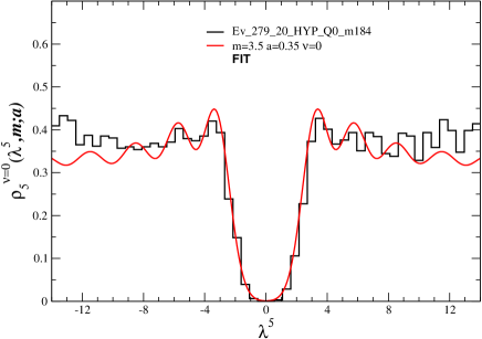
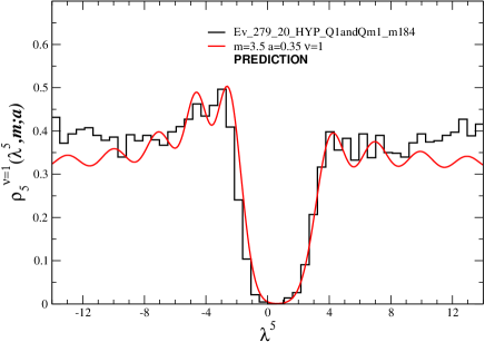
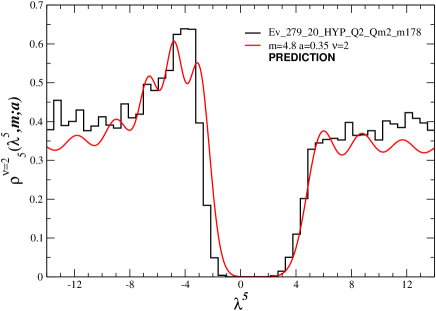
We first consider the $m_{0}=-0.184$ data with $\nu=0$. We make a fit and find the best values of $\hat{m}=3.5$, $\Sigma V=216$ and $\hat{a}_{8}=0.35$. (The fact that $\hat{m}$ and $\hat{a}$ takes the same value as for the $16^{4}$ lattice at $\beta_{Iw}=2.635$ is accidental.) For these values the analytic curve matches the data well over the lowest four eigenvalues, see the top panel of Figure 3.

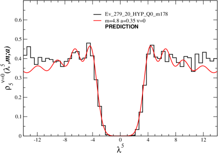
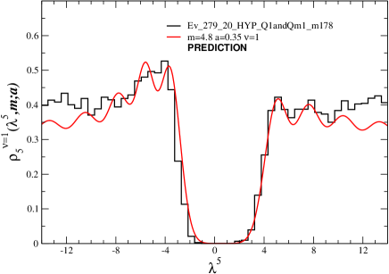
Given these values of $\hat{m}$ and $\hat{a}_{8}$ we then test the predicted density for $\nu=1$ against the data. As can be observed from the lower panel of Figure 3 this again works well for the lowest four eigenvalues. Finally, we consider also the higher mass data at the same value of the coupling. Since the lattice mass has changed from $m_{0}=-0.184$ to $m_{0}=-0.178$ we have $\delta m=0.006$ so that $\delta m\Sigma V=0.006*216=1.3$. Hence, we predict that the $\beta_{Iw}=2.79$ data with $m_{0}=-0.178$ should be matched with $\hat{m}=4.8$ and $\hat{a}=0.35$. As can be seen from Figure 4 this parameter free prediction works well for the $\nu=0$ as well as for the $|\nu|=1$ sector. Figure 5 compares the corresponding parameter free prediction for $|\nu|=2$ against the data.

We conclude that $W_{6}=W_{7}=0$ and $W_{8}>0$ is consistent with the $20^{4}$ lattice data with $\beta_{Iw}=2.79$ and that the mass scaling at fixed lattice spacing implied by WCPT works well. For the influence of $W_{6}$ and $W_{7}$ see below.

Figure 3: The eigenvalue density of $D_{5}$ for $\beta_{Iw}=2.79$, $V=20^{4}$ and $m_{0}=-0.184$ top: $\nu=0$ and bottom: $|\nu|=1$. For the $\nu=0$ data we find the best values $\hat{m}=3.5$, $\hat{a}_{8}=0.35$ and $\Sigma V=216$. With these values we then test the prediction against the $|\nu|=1$ data.

Figure 4: The eigenvalue density of $D_{5}$ for $\beta_{Iw}=2.79$, $V=20^{4}$ and $m_{0}=-0.178$ top: $\nu=0$ and bottom: $|\nu|=1$. We use the value $\Sigma V=216$ (found for $m_{0}=-0.184$) and $\delta m=-0.006$ to determine the value $\hat{m}=4.8$ for the $\beta_{Iw}=2.79$, $V=20^{4}$, $m_{0}=-0.178$ data. Since the coupling is unchanged also $\hat{a}_{8}=0.35$ is fixed by the previous fit. The parameter free predictions for $\nu=0$ and $|\nu|=1$ are then plotted against the data. We observe that the mass scaling at fixed lattice spacing works well.

Figure 5: The eigenvalue density of $D_{5}$ for $\beta_{Iw}=2.79$, $V=20^{4}$ and $|\nu|=2$ top: $m_{0}=-0.184$ and bottom: $m_{0}=-0.178$. The smooth curves are the parameter free predictions from WCPT (all parameters are fixed from the fit to the $\nu=0$, $m_{0}=-0.184$ data).

V.3 The $\hat{m}$ and $\hat{a}_{8}$ dependence

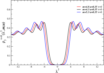
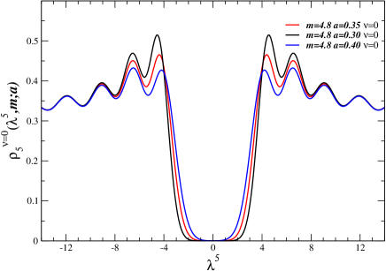
Above we have obtained best fits of the analytic prediction, Eq. (18), to the lattice data by varying $\hat{m}$ and $\hat{a}_{8}$. Here we demonstrate the strong sensitivity of the analytic predictions for the microscopic eigenvalue density of $D_{5}$ with fixed index to the values of $\hat{m}$ and $\hat{a}_{8}$. Figure 6 give examples of this strong dependence which allow for a precise determination of the best values for the match to the data. Figure 7 compares the best fit to the continuum, $a=0$, curve. In this way we estimate the error on $\hat{a}_{8}$ in our data sets to be at most $0.05$ and the error on $\hat{m}$ to be below $0.5$. With increased statistics on slightly larger lattices at slightly smaller lattice spacing it should be possible to determine $\hat{m}$ and $\hat{a}_{8}$ with high accuracy.

Figure 6: The dependence of the eigenvalue density of $D_{5}$ for $\nu=0$ on top: the quark mass $\hat{m}$ and on bottom: the lattice artifacts $\hat{a}_{8}$. The central (Red) line in both plots correspond to the (Red) analytic curve which is plotted against the data in the top panel of Figure 4.

Figure 7: The eigenvalue density of $D_{5}$ for $\nu=0$. Shown are the lattice data and best fit, previously displayed in the top panel of Figure 3, along with the $a=0$ result at the same value of $\hat{m}$. Clearly it is essential to include the order $a^{2}$ effects in WCPT in order to match the data. Note that scale on the $y$-axis is different from that in the other plots.

V.4 Effects of $W_{6}$ and $W_{7}$

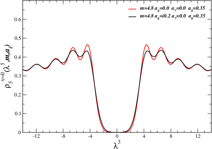
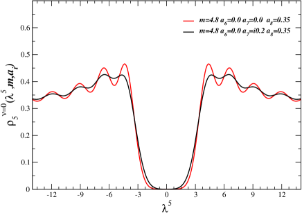
The effect of $W_{6}<0$ or $W_{7}<0$ is to smear out the analytic predictions so that the bumps in the curves become less pronounced. In Figure 8 we give an example of the effect of $\hat{a}_{6}^{2}$ and $\hat{a}_{7}^{2}$. The more oscillating curve in both plots corresponds to the curve in the top panel of Figure 4 which has $\hat{a}_{6}=\hat{a}_{7}=0$. As a less pronounced structure of the oscillations due to the individual eigenvalues is unfavored by the lattice data we conclude that $|\hat{a}_{6}^{2}|$ and $|\hat{a}_{7}^{2}|$ appear to be smaller than $0.01$. Note that $\hat{a}_{i}$ only enters as squares in the action (11), that is why it is natural to give the bound on the square.

Figure 8: The eigenvalue density of $D_{5}$ for $\nu=0$ top: the dependence on $\hat{a}_{6}$ and bottom: the dependence on $\hat{a}_{7}$. The more oscillating (Red) line in both plots has $a_{6}=a_{7}=0$ and corresponds to the (Red) analytic curve which is plotted against the data in the top panel of Figure 4. Both $\hat{a}_{6}^{2}<0$ or $\hat{a}_{7}^{2}<0$ tends to smear out the oscillations. Since the magnitude of the oscillations in the lattice data presented in Figure 4 is of the same magnitude as those in the analytic prediction with $\hat{a}_{6}=\hat{a}_{7}=0$ we can put an upper bound on these $|\hat{a}_{6}^{2}|,|\hat{a}_{7}^{2}|<0.01$.

V.5 Individual eigenvalue distributions

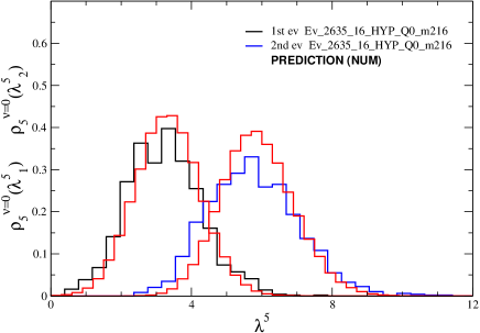
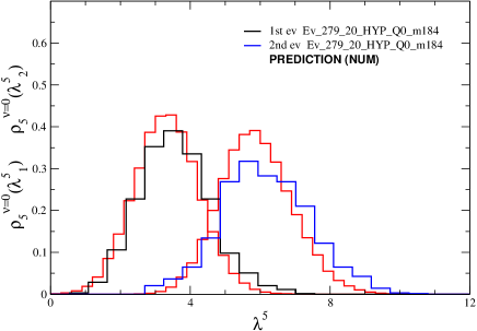
In order to understand in greater detail whether our lattice data match the predictions from WCPT and WRMT it is advantageous to consider the distributions of individual eigenvalues. As we do not have any simple expression available from the chiral Lagrangian approach, we will simply make use of the relation to Wilson chiral random matrix theory, and generate the distributions numerically. See Figure 9.

For the $\beta_{Iw}=2.635$ data on the $16^{4}$ lattice the first eigenvalue matches well that generated from WRMT. The second eigenvalue however is somewhat broader.

In the $\beta_{Iw}=2.79$ data from the $20^{4}$ lattice the first eigenvalue again matches well that generated from WRMT. This time the second eigenvalue is repelled from the first in a manner comparable to the one observed in the simulation of WRMT.

Figure 9: The distribution of the first (black) and second (blue) eigenvalue top: in the $16^{4}$ $\beta_{Iw}=2.635$ data set and bottom: in the $20^{4}$ $\beta_{Iw}=2.79$ data set. The (red) histograms show the first and second eigenvalue distribution in a WRMT simulation with $n=100$ and 100000 matrices.

V.6 The real eigenvalues of $D_{W}$

From the flow of $\lambda^{5}$ as a function of $m$ we have also determined the real eigenvalues of $D_{W}$ as well as their chiralities. This enables us to measure both the density of the real modes

$$\rho_{real}^{\nu}(\lambda^{W};a)=\left\langle\sum_{k}\delta(\lambda^{W}-\lambda^{W}_{k})\right\rangle$$ (27)

as well as the distribution

$$\rho_{\chi}^{\nu}(\lambda^{W};a)=\left\langle\sum_{k}\delta(\lambda^{W}-\lambda^{W}_{k}){\rm sign}\langle k|\gamma_{5}|k\rangle\right\rangle.$$ (28)

The analytic predictions for both these quantities are available, see KVZ for $\rho_{real}$ and DSV ; ADSV for $\rho_{\chi}$. The two distributions both merge to a $\nu$-fold $\delta$-function at the origin for $\hat{a}\to 0$.

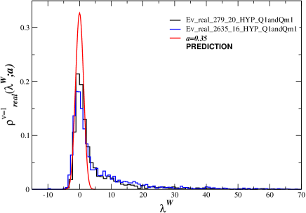
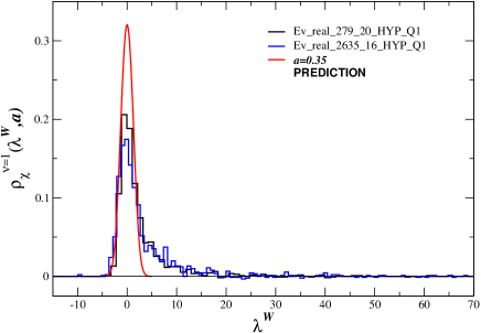
From the fit to $\rho_{5}$ we have already obtained the relevant values of $\Sigma V$, $\hat{m}$ and $\hat{a}$. This enables a highly nontrivial parameter free test of WCPT. In Figure 11 the parameter free analytic predictions are plotted along with the results from the lattice. Since accidentally the value $\hat{a}=0.35$ was obtained for both data sets we have combined the plots. For the plot we have rescaled the lattice eigenvalues, shown in Figure 10, by $\Sigma V$ (the value for which we obtained from the respective fits to $\rho_{5}$) and then shifted the eigenvalues by $\Sigma Vm_{0}-\hat{m}$. For the $20^{4}$ data with $m_{0}=-0.184$ and $\beta_{Iw}=2.79$ this reads $\Sigma Vm_{0}-\hat{m}=216(-0.184)-3.5=-43.2$ while for the $16^{4}$ data with $\beta_{Iw}=2.635$ and $m_{0}=-0.216$ it reads $\Sigma Vm_{0}-\hat{m}=157.5(-0.216)-3.5=-37.5$.

Figure 10: The distribution of the real modes of $D_{W}$ before subtraction of the bare mass and scaling of the axis.

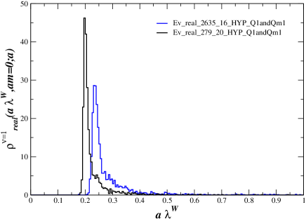
We observe that the scaling implied by WCPT is remarkable accurate. After the parameter free shift of the eigenvalues the center of the data peak is right at the origin as predicted by WCPT. Moreover, the width of the peak in both data sets is exactly of the right magnitude. We also note that the peak height in the data increases towards the analytic prediction when going from $16^{4}$ to $20^{4}$.

However, in the data there is an asymmetry of $\rho_{real}$ and $\rho_{\chi}$ which persist when going from $16^{4}$ to $20^{4}$. Moreover, the average number of real modes is predicted to be 1.017 by WRMT for $\nu=1$ and $\hat{a}=0.35$ KVZ , in the data we find 1.237 for the $16^{4}$ lattice and 1.185 for the $20^{4}$ lattice. That is, the average number of additional real modes is off by a factor of 10. We note, however, that this average number of additional real modes decrease by $22\%$ when going from $a=0.93$ fm on $16^{4}$ to $a=0.075$ fm on $20^{4}$.

The asymmetry of the distribution of the real eigenvalues is a clear signal that at the present volumes there are small real eigenvalues of $D_{W}$ which are not captured by leading order WCPT. In Anna it was observed that the eigenvectors corresponding to eigenvalues of $D_{W}$ which fall to the right of the main band have a strong tendency to be localized. Obviously such localized modes are not described by WCPT.

Figure 11: top: The distribution of the real modes. bottom: the distribution $\rho_{\chi}$ defined in Eq. (28). All parameters are fixed from the fits to $\rho_{5}$. The eigenvalue data are first rescaled by $\Sigma V$ and then shifted by $m_{0}\Sigma V-\hat{m}$ where $m_{0}$ is the lattice mass and $\hat{m}$ is the value obtained previously for this $m_{0}$.

VI Conclusions

The analytical predictions for the quenched microscopic spectral density of the Hermitian Wilson-Dirac operator have been compared to the low lying eigenvalues of Wilson fermions on the lattice. In this first study, we have demonstrated that the results given for fixed index of the Wilson-Dirac operator can be matched by the predictions from Wilson chiral perturbation theory with $W_{8}>0$ and $W_{6}=W_{7}=0$. We have successfully tested the finite volume scaling at fixed lattice spacing as well as the mass scaling as fixed lattice spacing predicted by Wilson chiral perturbation theory against the lattice data. The spectrum of $D_{5}$ in this way gives a very direct way of measuring the low-energy constants of Wilson chiral perturbation theory. Although these constants represent lattice artifacts, it is essential to know their values in order to extract the physical constants. Moreover, the detailed predictions can be used with advantage to understand how the spectrum can be made to retain its gap as simulations are pushed towards physical values and towards the continuum limit.

We emphasize that the assignment of index $\nu$ to a given gauge field configuration must be based on the spectral flow of the Hermitian Wilson-Dirac in order for the match to Wilson chiral perturbation theory to be valid. In the microscopic limit the analytic results predict that the real eigenvalues of $D_{W}$ are located in well separated regions. On the lattice, it should therefore be possible in a clean way to introduce a cut-off such that we consider only the physical branch of the spectrum. In support of this we have explicitly computed the real eigenvalues of $D_{W}$ and found that the bulk of the real eigenvalues follow the predictions from WCPT. However, we observed also an asymmetry of the distribution of the real eigenvalues not described by WCPT. For this reason some configurations that are difficult to classify remain in our samples. Similar concerns have been voiced already in the context of the overlap operator Anna , where localized modes that intuitively should play no role in the continuum limit nevertheless significantly deform the spectrum of the overlap operator at fixed $\nu$. We stress that such localized modes are not described by Wilson chiral perturbation theory. As such modes are more easily identified in the complex part of the spectrum of $D_{W}$ a careful and high-statistics study of the microscopic spectrum of the Wilson-Dirac operator which address this issue would provide a valuable test of Wilson chiral perturbation theory at presently realistic lattice spacings. The analytic prediction for the quenched microscopic eigenvalue density of $D_{W}$ in the complex plane has been presented very recently KVZ .

It is also possible to transform all analytical predictions for the microscopic spectral density of the Hermitian Wilson-Dirac operator into corresponding expressions for the pseudoscalar condensate $\langle\bar{\psi}\gamma_{5}\psi\rangle$, as discussed in Ref. Heller . It would be interesting to use this quantity to extract the Wilson low-energy constants.

To summarize we have demonstrated here that the theoretical predictions of Wilson chiral perturbation theory with $W_{6}=W_{7}=0$ and $W_{8}>0$ for the microscopic spectral properties of the Wilson-Dirac operator can be matched to lattice data. It would be most interesting to extend this quenched study to the physical case of two light flavors. The detailed theoretical predictions have been given recently SVdyn .

End note: We learned at the Lattice 2011 meeting that Albert Deuzeman, Urs Wenger and Jaïr Wuilloud have been investigating the same issues we have discussed here. We thank these authors for coordinating publication of results. Their paper is Ref. DWW .

Acknowledgments: We would like to thank Jac Verbaarschot, Anna Hasenfratz, Hidenori Fukaya, Christian Lang and Christof Gattringer for discussions. The work of K.S. was supported by the Sapere Aude program of The Danish Council for Independent Research.

References

- (1) L. Del Debbio, L. Giusti, M. Lüscher, R. Petronzio and N. Tantalo, JHEP 0602, 011 (2006) [hep-lat/0512021]; JHEP 0702, 056 (2007) [hep-lat/0610059].
- (2) S. R. Sharpe and R. L. Singleton, Phys. Rev. D 58, 074501 (1998) [hep-lat/9804028]; G. Rupak and N. Shoresh, Phys. Rev. 66, 054503 (2002), [hep-lat/0201019]; O. Bär, G. Rupak and N. Shoresh, Phys. Rev. D 70, 034508 (2004), [hep-lat/0306021]; S. Aoki, Phys. Rev. D 68, 054508 (2003) [arXiv:hep-lat/0306027]; S. Aoki and O. Bär, Phys. Rev. D 70, 116011 (2004) [arXiv:hep-lat/0409006].
- (3) S. R. Sharpe, Phys. Rev. D 74, 014512 (2006) [hep-lat/0606002].
- (4) P. H. Damgaard, K. Splittorff and J. J. M. Verbaarschot, Phys. Rev. Lett. 105, 162002 (2010). [arXiv:1001.2937 [hep-th]].
- (5) G. Akemann, P. H. Damgaard, K. Splittorff, J. J. M. Verbaarschot, Phys. Rev. D 83, 085014 (2011) [1012.0752 [hep-lat]].
- (6) G. Akemann, T. Nagao, [arXiv:1108.3035 [math-ph]].
- (7) M. Kieburg, J. J. M. Verbaarschot, S. Zafeiropoulos, [arXiv:1109.0656 [hep-lat]].
- (8) G. Akemann, P. H. Damgaard, K. Splittorff, J. J. M. Verbaarschot, PoS LATTICE2010, 079 (2010). [1011.5121 [hep-lat]].
- (9) K. Splittorff and J. J. M. Verbaarschot, arXiv:1105.6229 [hep-lat].
- (10) S. Itoh, Y. Iwasaki and T. Yoshie, Phys. Rev. D 36, 527 (1987).
- (11) A. Shindler, Phys. Lett. B672, 82-88 (2009). [0812.2251 [hep-lat]]; O. Bar, S. Necco, S. Schaefer, JHEP 0903, 006 (2009). [0812.2403 [hep-lat]]; S. Necco, A. Shindler, [1101.1778 [hep-lat]].
- (12) H. Leutwyler, A. V. Smilga, Phys. Rev. D46, 5607-5632 (1992).
- (13) R. G. Edwards, U. M. Heller and R. Narayanan, Nucl. Phys. B 535, 403 (1998) [hep-lat/9802016].
- (14) P. H. Damgaard, J. C. Osborn, D. Toublan and J. J. M. Verbaarschot, Nucl. Phys. B 547, 305 (1999) [hep-th/9811212].
- (15) K. Splittorff, J. J. M. Verbaarschot, Nucl. Phys. B683, 467-507 (2004). [hep-th/0310271].
- (16) K. Splittorff, J. J. M. Verbaarschot, Nucl. Phys. B757, 259-279 (2006). [hep-th/0605143].
- (17) S. Aoki, Phys. Rev. D30, 2653 (1984).
- (18) G. Akemann, P. H. Damgaard, U. Magnea and S. Nishigaki, Nucl. Phys. B 487, 721 (1997) [hep-th/9609174].
- (19) J. C. Osborn, Nucl. Phys. Proc. Suppl. 129, 886 (2004) [hep-lat/0309123].
- (20) Y. Iwasaki, UTHEP-118.
- (21) S. Takeda, et al., Phys. Rev. D70, 074510 (2004) [arXiv:hep-lat/0408010].
- (22) S. Necco, Nucl. Phys. B683, 137 (2004) [arXiv:hep-lat/0309017].
- (23) A. Hasenfratz and F. Knechtli, Phys. Rev. D64, 034504 (2001) [arXiv:hep-lat/0103029].
- (24) A. Hasenfratz, R. Hoffmann and S. Schaefer, JHEP 0711, 071 (2007) [0709.0932 [hep-lat]].
- (25) K. M. Bitar, U. M. Heller and R. Narayanan, Phys. Lett. B 418, 167 (1998) [hep-th/9710052].
- (26) A. Deuzeman, U. Wenger and J. Wuilloud, arXiv:1110.4002 [hep-lat].