Interspecific competition underlying mutualistic networks
Abstract
Multiple classes of interactions may exist affecting one another in a given system. For the mutualistic networks of plants and pollinating animals, it has been known that the degree distribution is broad but often deviate from power-law form more significantly for plants than animals. To illuminate the origin of such asymmetry, we study a model network in which links are assigned under generalized preferential-selection rules between two groups of nodes and find the sensitive dependence of the resulting connectivity pattern on the model parameters. The nonlinearity of preferential selection can come from interspecific interactions among animals and among plants. The model-based analysis of real-world mutualistic networks suggests that a new animal determines its partners not only by their abundance but also under the competition with existing animal species, which leads to the stretched-exponential degree distributions of plants.
pacs:
87.23.Kg, 05.40.-a, 89.75.HcDiverse interactions and dependencies among nonidentical elements are characteristic of complex systems mucha10 ; buldyrev10 ; ahn10 . Ecological systems are a prototypical example, in which numerous species interact via predation, herbivory, mutualistic support, competition, cooperation, and so on, and their network structure and function have attracted much attention pascual05 ; bascompte10 ; montoya06 ; saavedra09 ; bastolla09 . The mutualistic relation between two species is beneficial for the survival and reproduction of both of them such as animal pollinators and flowering plants. Given numerous species of plants and insects, producing nectar with different composition and flavor and carrying a wide range of preference and capacities, respectively, the establishment of individual mutualistic relationship depends on specific needs and qualification. Nevertheless, the global organization of the mutualistic plant-pollinator networks exhibits common features jordano03 ; bascompte03 ; vazquez05 ; guimaraes07 ; santamaria07 ; guimaraes07 ; maeng11 ; campbell11 . The degrees of plant and animal species are distributed broadly in general, but their distributions often deviate from a power-law form, more significantly for plant species: While the degree distribution of animals are close to power laws, those of plants are of truncated power-law, exponential, or stretched-exponential form jordano03 ; guimaraes07 ; maeng11 . Biological matching, species abundance, and the difference between the numbers of animals and plants may bring such deviation from scale invariance jordano03 ; vazquez05 ; guimaraes07 , which, however, remains to be addressed further santamaria07 . Interestingly, mutualistic networks have their topological features distinguished from trophic networks particularly in their nestedness and modularity, which is related to the stable architecture varying with the type of interaction thebault10 .
To gain insight into the underlying mechanism of mutualistic community formation, here we propose and study a simple growing bipartite network model and apply it to analyze real-world mutualistic networks. The model is based on a generalized preferential-selection rule, being an extension of the model in Ref. guimaraes07 . From the nestedness and broad degree distributions identified in lots of mutualistic communities, the preferential selection barabasi99 has been expected to play a role in their evolution jordano03 ; guimaraes07 ; santamaria07 ; thebault10 . Our model provides a unified picture of evolving mutualistic communities. The nonlinear preferential selection reflects the impact of individual characteristics and interspecific interactions on determining symbionts. Fitting the model prediction to empirical data, we discover a pattern of interspecific interaction affecting the architecture of mutualistic networks. While a new animal species is attracted to a plant species with high abundance and thus with many pollinators already, it should compete with the existing pollinators. As a result, the chance to find a plant species with a large number of pollinators is not as high as expected, which is shown to cause the degree distribution of plants to take a stretched-exponential form.

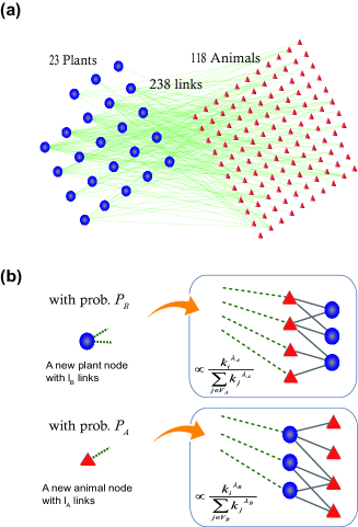
To be specific, we consider plant-pollinator mutualistic networks as in Fig. 1 (a), in which each node represents a species of either animal () type or plant () type and some pairs of nodes of the opposite types are connected representing their mutualistic relationship. A growing bipartite network (GBN) model defined below and also sketched in Fig. 1(b) guimaraes07 ; ramasco04 ; goldstein05 ; lambiotte05 illustrates the topological evolution of the plant-pollinator networks. Initially there are nodes of type and nodes of type , all pairs of nodes of the opposite types being connected. At each time step, a new node of type arrives with probability , where . The new node of type () are linked to partners of type that are selected with the probability proportional to the th power of their degrees. Iterating these procedures up to time , one obtains a bipartite network of nodes of type and nodes of type on average.
The degree-based preferential selection by a new species is assumed in this model and can be motivated as follows. In case that a new species appears by speciation from an existing one, it can be assumed to inherit the mutualistic interactions of the ancestor species, as the protein interactions are inherited by duplicated genes berg04 . Then, the more partners an existing species has, the higher the chance to have a new mutualistic partner speciated from one of its old partners is. Also, if we assume that a new species in a community, appearing by either speciation or migration, selects randomly its partner organisms, the new species will be more likely to form a mutualistic relationship with a more abundant species due to the existence of more organisms of the species. Given that the number of mutualistic partners - degree - of a species is positively correlated with the abundance of the species, the degree-based preferential selection is expected to work in this case, too.
Restricted resources provided by one type of species may draw competition among the other type of species, which can give rise to the nonlinear preferential selection. For a new animal species , let us assign to each pollinator of each plant , which can be negative or positive depending on the significance of the competitive interaction between and relative to the abundance of plant . The sum of those interaction coefficients over can be a measure of the chance that can occupy the plant . When the sum is negative, the plant will not be selected. Thus, the selection probability of plant with degree will be proportional to , which can be viewed as the effective degree of for . On ensemble average, and the selection probability will be proportional to if . On the other hand, if , , in which is the random-walk dimension varying with the distribution and correlation of ’s hughesbook . Both cases are considered in our model with . Similarly, a new plant can be complementary or substitutable for each pollinator nurturing each animal , which leads the probability of animal to pollinate to scale with linearly or sublinearly. The impact of such nonlinear preferential attachment has been investigated for unipartite growing networks krapivsky00 and the preferential-selection exponent, , has been measured empirically e.g., for the Internet satorras01 .
The mean number of nodes of degree and type evolves with time as krapivsky00
| (1) |
where . We use and to indicate the opposite types of nodes such that or . In the long-time limit , is proportional to time such that , where is the degree distribution for type . It is inserted into Eq. (1) to yield
| (2) |
where the constant is given by
| (3) |
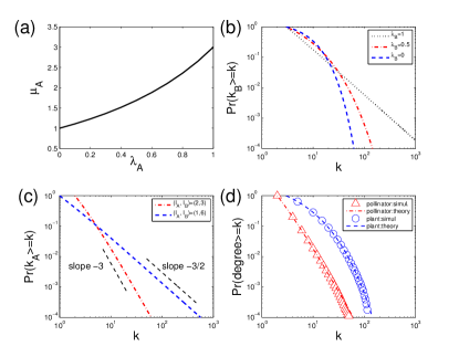
It is worthy to note that Eq. (1) has the Kramers-Moyal coefficients that are identical at all orders riskenbook , preventing a truncated expansion. While and are engaged in determining and , respectively, both and depend on , and , leading and to be coupled. Note that at and at (Fig. 2 (a)).

The dependence of the degree distributions on the parameters is manifested in its asymptotic behavior:
| (6) | |||||
with
| (7) |
Remarkably, changes from a power-law to a stretched-exponential form as deviates from as in the example in Fig. 2 (b) krapivsky00 . For , the degree exponent of power-law degree distributions varies continuously not only with the fraction of nodes of the two types and guimaraes07 but also with the initial numbers of links and (Fig. 2(c)). Such sensitive dependence in bipartite networks enables us to look into the microscopic details through the global organization of bipartite systems. The numerical solutions are in agreement with model simulations as in Fig. 2(d).
If and are integers, the possible value of in Eq. (7) are restricted, which is not the case in real-world networks. Considering as the mean number of initial links, we let a new node of type assigned or links with probability or , respectively. is the largest integer not larger than . Then Eq. (6) remains to be true, with a slight change of from Eq. (2) to
| (8) |
with .

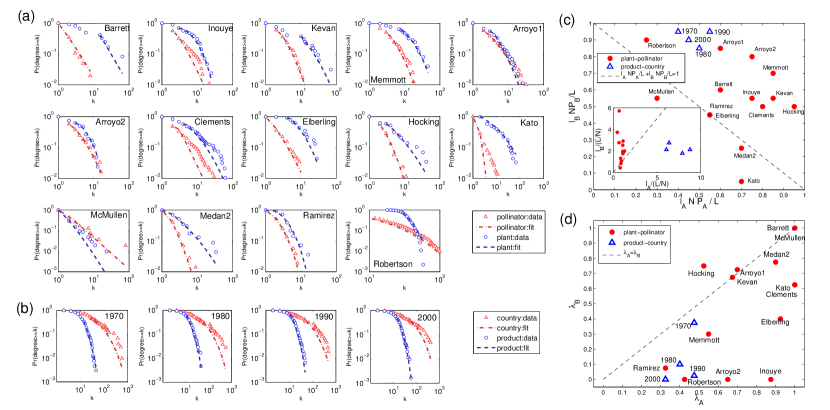
We fitted the model predictions of the degree distributions in Eq. (8) to those of real plant-pollinator networks iwdb by adjusting , and through the combined use of the maximum-likelihood estimation and the Kolmogorov-Smirnov statistic clauset09 . The fitted degree distributions are in good agreement with data as shown in Fig. 3 (a). The initial number of links of plants turns out to be much larger than that of animals probably due to there being more animal than plant species; their normalized values, and , are distributed uniformly as shown in Fig. 3 (c). Most importantly, the preferential-selection exponents show a significant asymmetry: in most networks as shown in Fig. 3 (d). This implies the significantly strong competition between a new animal and existing pollinators contrary to the relatively weak competition between plants. Thus one can see that the restriction on the number of available plant species is a more crucial factor in shaping the mutualistic community than the restriction on available animal species, possibly related to the difference in their survival and reproduction rates. Consequently, plants with large degrees have the advantage of their high abundance screened by the competition between animals characterized by less than , which leads the degree distribution to take a stretched-exponential form . We remark that these observations are not the case for “Hocking” in Fig. 3 (d), for which it has been reported in Ref. hocking68 that the competition between plants is more significant than between pollinators, implying .
To check further the robustness of our results, we analyzed the product-country networks representing which country exports which product hidalgo07 . Both the prevalence of a product and the wealth of each country depend on trade volume and thus a country (A) and a product (B) may have mutualistic relation in the global economic ecosystems. Although and contrasted to plant-pollinator networks, we find again that suggesting the same patterns of competition among countries as among pollinators.
In conclusion, we found that the connectivity pattern of bipartite networks is sensitively dependent on model details. Such sensitivity can be of potential use in controlling transport and epidemic affected by the connectivity in multiconnected systems and, in the present work, allowed us to illuminate the interaction patterns hidden under the bipartite architecture of mutualistic networks. The stretched-exponential form of the degree distribution of plants is shown to be driven by the significant competition between pollinating animals, which is true also for countries in economic mutualistic networks. Our results demonstrate the importance of taking into account the cross-talk between different types of links interwoven in a system in order to understand and predict its properties. While we focused on the global network architecture of mutualistic communities, it is highly desirable to extend our model to account for the population dynamics and diverse interspecific interactions.
Acknowledgements.
We thank the anonymous reviewers for helpful comments. This work was supported by Basic Science Research Program through the National Research Foundation of Korea (NRF) funded by the Ministry of Education, Science and Technology [Grants No. 2011-0003015 (J.W.L) and No. 2011-0003488 (D.-S.L)]. D.-S.L. acknowledges the TJ Park Foundation for support.References
- (1) P.J. Mucha, T. Richardson, K. Macon, M.A. Porter, and J.-P. Onnela, Science 328, 876 (2010).
- (2) S. V. Buldyrev, R. Parshani, G. Paul, H. E. Stanley, and S. Havlin, Nature 464, 1025 (2010).
- (3) Y.-Y. Ahn, J.P. Bagrow, and S. Lehmann, Nature 466, 761 (2010).
- (4) see e.g., M. Pascual and J.A. Dunne, Ecological Networks: Linking Structure to Dynamics in Food Webs (Oxford Univ. Press, new York, 2005) and references therein.
- (5) J.M. Montoya, S.L. Pimm, and R.V. Solé, Nature 442, 259 (2006).
- (6) J. Bascompte, Science 329, 765 (2010).
- (7) S. Saavedra, F. Reed-Tsochas, and B. Uzzi, Nature 457, 463 (2008).
- (8) U. Bastolla, M.A. Fortuna, A. Pascual-Garcia, A. Ferrera, B. Luque, and J. Bascompte, Nature 458, 1018 (2009).
- (9) J. Bascompte, P. Jordano, C.J. Melián, and J.M. Olesen, Proc. Nat’l Acad. Sci. USA 100, 9383 (2003).
- (10) P. Jordano, J. Bascompte, and J.M. Olesen, Ecol. Lett. 6, 69 (2002).
- (11) P.R. Guimarães Jr., G. Machado, M.A.M. de Aguiar, P. Jordano, J. Bascompte, A. Pinheiro, and S.F. dos Reis, J. Theo. Biol. 249, 181 (2007).
- (12) S.E. Maeng and J.W. Lee, J. Kor. Phys. Soc. 58, 851 (2011).
- (13) C. Campbell, S. Yang, R. Albert, and K. Shea, Proc. Nat’l Acad. Sci. USA 108, 197 (2010).
- (14) D.P. Vázquez, Oikos 108, 421 (2005).
- (15) L. Santamaría and M.A. Rodríguez-Gironés, PLoS Biol. 5, e31 (2007).
- (16) E. Thébault and C. Fontaine, Science 329, 853 (2010).
- (17) A.-L. Barabási and R. Albert, Science 286, 509 (1999).
- (18) J.J. Ramasco, S.N. Dorogovtsev, and R. Pastor-Satorras, Phys. Rev. E 70, 036106 (2004).
- (19) M.L. Goldstein, S.A. Morris, and G.G. Yen, Phys. Rev. E 71, 026108 (2005).
- (20) R. Lambiotte and M. Ausloos, Phys. Rev. E 72, 066107 (2005).
- (21) J. Berg, M. Lässig, and A. Wagner, BMC Evol. Biol. 4, 51 (2004).
- (22) B.D. Hughes, Random Walks and Random Environments (Oxford University, New York, 1995).
- (23) P.L. Krapivsky, S. Redner, and F. Leyvraz, Phys. Rev. Lett. 85, 4629 (2000).
- (24) R. Pastor-Satorras, A. Vázquez, and A.Vespignani, Phys. Rev. Lett. 87, 258701 (2001).
- (25) H. Risken, The Fokker-Planck Equation (Springer, Berlin, 1989).
- (26) http://www.nceas.ucsb.edu/interactionweb/resources.html. The reference of each data-set is also given in the Web site.
- (27) A. Clauset, C.R. Shalizi, and M.E.J. Newman, SIAM Review 51, 661 (2009).
- (28) B. Hocking, Oikos 19, 359 (1968).
- (29) C.A. Hidalgo, R. B. Klinger, A.-L. Barabási, R. Hausmann, Science 317, 482 (2007).
- (30) H. Elberling and J.M. Olesen, Ecography 22, 314 (1999).