When Shape Matters: correcting the ICFs to derive the chemical abundances of bipolar and elliptical PNe

Abstract

The extraction of chemical abundances of ionised nebulae from a limited spectral range is usually hampered by the lack of emission lines corresponding to certain ionic stages. So far, the missing emission lines have been accounted for by the ionisation correction factors (ICFs), constructed under simplistic assumptions like spherical geometry by using 1-D photoionisation modelling.

In this contribution we discuss the results (Gonçalves et al. 2011, in prep.) of our ongoing project to find a new set of ICFs to determine total abundances of N, O, Ne, Ar, and S, with optical spectra, in the case of non-spherical PNe. These results are based on a grid of 3-D photoionisation modelling of round, elliptical and bipolar shaped PNe, spanning the typical PN luminosities, effective temperatures and densities.

We show that the additional corrections –to the widely used Kingsburgh and Barlow (1994) ICFs– are always higher for bipolars than for ellipticals. Moreover, these additional corrections are, for bipolars, up to: 17% for oxygen, 33% for nitrogen, 40% for neon, 28% for argon and 50% for sulphur. Finally, on top of the fact that corrections change greatly with shape, they vary also greatly with the central star temperature, while the luminosity is a less important parameter.

1 A brief history the derivation of nebular abundances

Accurate ionization correction factors are the key to determining reliable elemental abundances for ionized nebulae, for which it is usually the case that only one or two ionization stages of a given element can be observed.

[Torres-Peimbert & Peimbert (1979), Torres-Peimbert & Peimbert (1979)] already proposed and used ICFs to obtain total abundances of PNe, a number of years ago. Their ICFs were based on the correlations of the ionic abundances of different elements, like those shown in their Fig. 3, for $\log(Ne^{++}/O^{++})$ and $\log(Ar^{++}/O)$ respect to $\log(O^{++}/O)$. Other ICF schemes were proposed since then, being the [Kingsburgh & Barlow (1994), Kingsburgh & Barlow (1994)](KB94) the main one.

The other common approach to derive total abundances is the one in which the empirical (ICF) abundances are the input abundances in the photoionisation model fitting of a particular nebula for which a number of other input parameters are available ([Stasińska 2002, Stasińska 2002]). In this case the empirical abundances are varied until the predicted emission-line ratios (and emission-line maps) match the observations (see, for instance, [Gonçalves et al. 2006, Gonçalves et al. 2006]).

2 Our grid of 3-D models for bipolar and elliptical PNe

For this study we use mocassin (a fully 3-D Monte Carlo photoionisation code): i) which treats the basic ionization and recombination (including charge-exchange and dielectronic recombination) physical processes; ii) in which the stellar and diffuse radiation fields are treated self-consistently; and iii) is completely independent of the assumed nebular geometry ([Ercolano et al. (2003), Ercolano et al. (2005), Ercolano et al. (2008), Ercolano et al. 2003, 2005, 2008)].

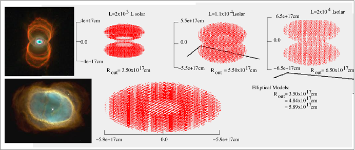
Figure 1: The density maps of the 3-D models. The outer radius of all the 6 B and E geometries adopted are also given. Top: the size variation with luminosity, for bipolars. Bottom: the largest elliptical density distribution.

The space parameter to be explored was defined following the previous studies of [AB97, Alexander & Balick (1997)], [Perinotto et al. (1998), Perinotto et al. (1998)], [Gruenwald & Viegas (1998), Gruenwald & Viegas (1998)] and [Morisset & Stasińska (2008), Morisset & Stasińska (2008)]. We explored blackbody central star temperature ($T_{eff}$) and luminosity (L) ranges similar to theirs, with: three different L ($2\times 10^{3}$ L_⊙, $1.1\times 10^{4}$ L_⊙ and $2\times 10^{4}$ L_⊙); and varying the $T_{eff}$ from $50\times 10^{3}$ to $200\times 10^{3}$ (K) in steps of 25,000 K. The set of chemical abundances of the models are two, those of non-type I and type I PNe, as defined by KB94, for He, C, N, O, Ne, Ar and S. Bipolar (B) and elliptical (E) bright rim geometries are adopted (see Figure 1), with constant electron densities ($N_{e}$) of $3\times 10^{3}$ cm^-3 within the shells, and a much higher constant $N_{e}$ in the torus of the bipolar models ($N_{e}$(torus)=6$\times$$N_{e}$(lobes), [TA09, Tafoya et al. 2009]). Finally, the inner and outer radius are varied in order to keep all models radiation bounded. As a consequence the higher the luminosity, the larger the nebula.

3 Results and highlighting remarks

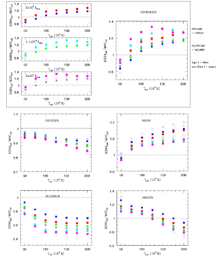
Figure 2: The variation of the KB94_ICF to MOC_ICF ratio for N, O, Ne, S and Ar with $T_{eff}$, L, chemical type and morphology. The 3 luminosities are show one by one, for nitrogen, in the top-left panel and then all together in the top-right one. Red (dark blue), white blue (green) and magenta (grey) represent the $2\times 10^{3}$ L_⊙, $1.1\times 10^{4}$ L_⊙ and $2\times 10^{4}$ L_⊙ elliptical (bipolar) models, respectively. The same colors apply to the other elements. Squares are for bipolar, while circles are for elliptical PNe, being the empty symbols for non-type I and the filled ones for type I PNe models. The doted line indicates the total agreement between the two ICFs, therefore points above (below) it indicate over (under) estimation of the true ionization correction factor that would completely account for the total chemical abundances of these elements.

Remembering that no ICFs are needed for He/H (the exception would be the very low-excitation PNe), we discuss only the results for O/H, N/H, Ne/H, S/H, and Ar/H (hereafter, we use X, instead of X/H, as the total abundance of a given element). The reader is referred to the KB94’s work to check the set of ICFs we use for the present analysis, that is restricted to the equations valid when optical (only) spectra are available. Namely, these are equations (A1), (A9), (A28), (A30), and (A36) of their Appendix A.

In our study, first, the line intensities given by mocassin for the 126 different models (whose parameters are given above) are used to obtain the He and the ionic abundances. Second, the KB94’s ICF, KB94_ICF, are calculated based on the optical emission-line ratios (ions). Third, as mocassin models return the ionic fractions, the true ionization correction factors, MOC_ICF, are obtained. And, finally, the ratio between the two ICFs tell us which are the additional corrections we should apply to the KB94 scheme in order to derive more robust chemical abundances for bipolar and elliptical PNe.

Our results are explained in Figure 2. It is straightforward to notice that none of the KB94 ICFs can recover the true abundances of bipolar (previously discussed by [Gruenwald & Viegas (1998), Gruenwald & Viegas (1998)] in a 3-D fashion, but only for nitrogen) and elliptical PNe. For $T_{eff}$ higher than $\sim$60$\times 10^{3}$ K, nitrogen and neon are always overestimated by the KB94 prescriptions, while oxygen and sulphur are under-estimated within the full range of effective temperatures, and argon goes from over- to under-estimation at about 150$\times 10^{3}$ K.

We can summarise the main results so far obtained for the discrepancies between ICF and true abundances as follows.

(1) The discrepancies vary with effective temperature as much as with shape, and they also change with luminosity and chemical type.

(2) The discrepancies are in general higher for bipolars than for ellipticals.

(3) In the worst cases, these discrepancies amount to, for bipolars (ellipticals):

- up to 33 (19)% for N (mainly over estimated);

- up to 17 (13)% for O (under estimated);

- up to 40 (40)% for Ne (mainly over estimated);

- up to 55 (50)% for S (under estimated); and

- up to 28 (24)% for Ar (either under or over estimated).

As a matter of fact, we are also studying the ICFs for round (spherically symmetric nebulae), since the approach we adopted here allow us to estimated the discrepancies that appear due the variation of L and $T_{eff}$ for simple morphological cases as well. Its clear from our spherically symmetric models that KB94 ICFs should be revisited also in the case of round PNe.

And, last but not least, the variation of ICF with temperature and luminosity can be more simply thought of as a variation with excitation class (although with some scatter). The complete discussion, as well as a set of equations for the corrections of the different morphologies, will be publish elsewhere soon (Gonçalves et al. 2011, in prep.).

References

- [Ercolano et al. (2003)] Ercolano B., Barlow M. J., Storey P. J., & Liu X.-W. 2003, MNRAS, 340, 1136
- [Ercolano et al. (2005)] Ercolano B., Barlow M. J., & Storey P. J. 2005, MNRAS, 362, 1038
- [Ercolano et al. (2008)] Ercolano B.,Young P. R., Drake J. J., & Raymond J. C. 2008, ApJS, 175, 534
- [Gonçalves et al. 2006] Gonçalves D. R., Ercolano B., Carnero A., Mampaso A., & Corradi R. L. M. 2006, MNRAS, 365, 1039
- [Gruenwald & Viegas (1998)] Gruenwald R., & Viegas S. M. 1998, ApJ, 501, 221
- [Kingsburgh & Barlow (1994)] Kingsburgh R. L., & Barlow M. J. 1994, MNRAS, 271, 257
- [Morisset & Stasińska (2008)] Morisset C., & Stasińska G. 2008, RMxAA, 44, 171
- [Perinotto et al. (1998)] Perinotto M., Kifonidis K., Schoenberner D., & Marten H. 1998, A&A, 332, 1044
- [Stasińska 2002] Stasińska G. 2002, in Cosmochemistry: The melting pot of the elements. XIII Canary Islands Winter School of Astrophysics. Eds. C. Esteban, R. J. García López, A. Herrero, F. Sanchéz