Response to “Comment on ‘Resolving the $180^{\circ}$ Ambiguity in Solar Vector Magnetic Field Data: Evaluating the Effects of Noise, Spatial Resolution, and Method Assumptions’ ”

Abstract

We address points recently discussed in mg2011 in reference to ambigworkshop2. Most importantly, we find that the results of mg2011 support a conclusion of ambigworkshop2: that limited spatial resolution and the presence of unresolved magnetic structures can challenge ambiguity-resolution algorithms. Moreover, the findings of both ambigworkshop1 and ambigworkshop2 are confirmed in mg2011: a method’s performance can be diminished when the observed field fails to conform to that method’s assumptions. The implication of boundaries in models of solar magnetic structures is discussed; we confirm that the distribution of the field components in the model used in ambigworkshop2 is closer to what is observed on the Sun than what is proposed in mg2011. It is also shown that method does matter with regards to simulating limited spatial resolution and avoiding an inadvertent introduction of bias. Finally, the assignment of categories to data-analysis algorithms is revisited; we argue that assignments are only useful and elucidating when used appropriately.

1 Introduction

sec:intro

The interpretation of remotely-observed solar polarimetric data requires algorithms to manipulate the data in order to prepare them for physical analysis. In order to produce a map of photospheric vector magnetic field, one must solve an inherent degeneracy in the direction of the inferred magnetic field perpendicular to the observer’s line of sight. Recently, efforts have been made to test the performance of available algorithms using “hare & hound” exercises that depend on synthetic data, for which the answer is known and performance can be evaluated quantitatively [Metcalf et al. (2006), Leka et al. (2009b)]. Ambiguity-resolution algorithms may seem fairly esoteric, yet provide intriguing windows into assumptions and details of observational data which are all too often made without acknowledgment or full understanding. For example, ambigworkshop1 showed that even the simplest “potential-field acute-angle” methods provide different solutions due to (seemingly) minor differences in implementation.

“Hare & hound” methods are only as good as the synthetic “hare” data. The best examples are constructed to separately test specific aspects of observational data, and the influences of underlying assumptions in the algorithms. Recently, mg2011 (MG2011) has questioned one “hare” used in ambigworkshop2 (LE2009) and the conclusions drawn from it. To test several aspects, including the effects of limited spatial resolution on ambiguity resolution algorithms, a potential-field construction nicknamed the “Flowers” model was devised in LE2009 to include small spatial scale structures that became unresolved after manipulations were performed to simulate the effects of smaller telescope aperture. A counter-model was proposed by MG2011 with the same vertical field, $B_{\rm z}$ on the boundary but a very different construction for $B_{\rm h}$, the horizontal field component; following MG2011, we refer to this as the “semi-infinite” model. (The models are constructed at disk-center; aside from subtle curvature issues that are beyond the scope of this response, the vertical field component is interchangeable with the line-of-sight or “longitudinal” component $B_{\rm long}$, and the horizontal field is interchangeable with the “transverse” component $B_{\rm trans}$, caveat the ambiguity-resolution.) Interested readers are referred to ambigworkshop2 and mg2011 for details; all data are publicly available.

The results of MG2011 help clarify a conclusion reached in LE2009, although we disagree with several of the specific claims made in the former. In this Response, we address four specific topics of particular importance. The results for the semi-infinite case of MG2011 in the context of limited spatial resolution are discussed, and we argue that there is no contradiction to the conclusions made by LE2009 (Section sec:res). We reinforce the reasons the “Flowers” test case was used in place of the semi-infinite model (Section sec:flowers), and the importance of properly simulating the effects of limited spatial resolution (Section sec:rebin). Finally, we discuss the distinctions made in MG2011 between “physics-based” and “optimization” methods for ambiguity resolution (Section sec:methods), and argue that the best performing methods are both “physics-based” and perform “optimization”.

2 Clarifying The Effects of Limited Spatial Resolution vs. Model Assumptions on Ambiguity Resolution Algorithms for the Flowers Model

sec:res

Testing the performance of algorithms requires an understanding of both the algorithms (the “hounds”) and the data used for evaluating the performance (the “hares”). Ideally, one challenge is presented to the algorithms at a time so as to disentangle cause and effect. Three challenges were presented in LE2009: photon noise, spatial resolution, and model assumptions. The “Flowers” model was used for the latter two challenges.

MG2011 disputes the conclusions of LE2009 about the role limited spatial resolution plays in the performance of ambiguity resolution algorithms. It is important to note that LE2009 did not claim that limited spatial resolution alone was responsible for the failure of algorithms in all areas of the “Flowers” case.

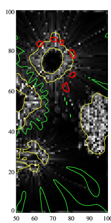
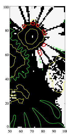
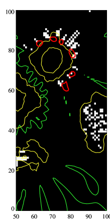
Figure 1.: Detail (right half) of select figures from LE2009 for bin-30 ($0.9^{\prime\prime}$): (Left) the parameter $\mathcal{D}$ (greyscale) from Figure 8 of LE2009, indicating “the degree to which the lack of spatial resolution affects the field” (LE2009). Green contour is the magnetic neutral line, yellow is a smoothed contour at $\mathcal{D}=0.25$, indicating a level of moderate impact, and red contours indicate locations of “azimuth centers”. Middle: the graphic representation of success/failure (black/white) for solution “KDP” from Figure 11 of LE2009, for bin-30 ($0.9^{\prime\prime}$), with same contours. Right: same representation for the solution “ME0”.fig:Dfig

In fact, most of the “Flowers” field is spatially resolved, even after binning by a factor of 30, with the notable exceptions of the “plage” area (centered at $[95,45]$ in Figure fig:Dfig), and some regions within the “sunspots”; this is clarified in Figure fig:Dfig, based on Figure 8 of LE2009. Where the parameter $\mathcal{D}$ is enhanced, the smallest-scale structures are located, although note that $\mathcal{D}$ is weighted by field strength. These areas can be expected to suffer due to degraded resolution.

The plage area has the smallest spatial scales, very enhanced $\mathcal{D}$, and was problematic for all methods applied to the Flowers model field. This area is precisely the region where poor results were also found in MG2011 by algorithms applied to the semi-infinite case, as evident from the statement

“Minor inconsistencies (white areas) refer exclusively to the “plage” area in the case of full resolution. For limited resolution, problems in the “plage” area seem to be enhanced, at least for the $0.3^{\prime\prime}$-per-pixel case (Figures 5(b) and 5(e) and, in addition, some minor problems occur in areas of strong gradients in the magnitude and orientation of the transverse field (Figure 1(e)) due to the lost structure.”

Similarly, “strong gradients in the magnitude and orientation of the transverse field” indicate the presence of small spatial scales. The “minor inconsistencies” even at full resolution are likely to be a result of the very small spatial scales (while resolved, they are presented on a discrete grid in the full-resolution model(s)) and possibly the discrepancy between the method used for the boundary computation (Green’s function for the “semi-infinite” case) and the FFT-based potential-field computation used in both algorithms highlighted in MG2011. In either case, this effect becomes more pronounced when the spatial resolution is degraded, as MG2011 pointed out for the semi-infinite case. Indeed, a second area of very small structures (the “ring” of azimuth centers highlighted in Figure fig:Dfig; see LE2009 and MG2011 for details) also proved troublesome for some algorithms, including in some instances propagating erroneous solutions.

Outside of the ring of azimuth centers in this top-left “sunspot”, however, the Flowers model is spatially resolved, and was constructed to test the susceptibility of algorithms to their inherent model assumptions. Potential-field acute-angle methods fail in this area (see Figure fig:Dfig, middle), as did most algorithms which compute a comparison field from the $B_{\rm z}$ boundary; other algorithms performed better (see Figure fig:Dfig, right). As such, this part of “Flowers” did not acutely test algorithms’ performance with spatial resolution degradation. The NonPotential Field Calculation method (NPFC, see Section sec:methods [Georgoulis (2005)]) fails in this area of the Flowers test case not due to worsening spatial resolution, but rather due to an assumption which is inconsistent with the model field, or possibly another aspect of the algorithm (such as the smoothing operator that may propagate erroneous solutions from regions where unresolved structure is an issue).

Thus there is no contradiction between the results of MG2011 and LE2009: spatially unresolved structures can cause problems for ambiguity resolution algorithms, even when the assumptions relied upon in the algorithms are satisfied by the underlying model (or observed) field. And MG2011 confirms what was stated in LE2009 (Section 4.3, referring to ambigworkshop1), “As in Paper I we find many methods perform poorly when the underlying field violates the assumptions being made.”

3 The Use of Boundaries in Models of the Solar Atmosphere

sec:flowers

One of the main objections raised in MG2011 to the “Flowers” case in LE2009 is the following (emphasis his):

“The chosen limited-resolution (‘flowers’) magnetograms, however, exhibited a feature that effectively disabled most disambiguation methods: the magnetic field vector was defined only within a narrow layer of $0.18^{\prime\prime}$ above the perceived ‘photosphere’, i.e., the plane on which disambiguation was tested.”

The “Flowers” model was only computed between the two boundaries (see LE2009 for a full description). However, it is straightforward to extend the definition to a semi-infinite space above the second boundary. Since ambiguity resolution algorithms only typically have the observed field on a single surface to work with, there was no reason to compute the field elsewhere.

Regarding the use of an upper boundary, MG2011 further contends,

“As sakurai89 puts it, one must have a physical reason for choosing a finite volume. This is the core of the problem with the finite-size magnetic structure of LE2009: other than computational convenience, there are no physical reasons dictating its selection.”

We agree with the sentiment expressed by sakurai89. The second boundary of the “Flowers” model was not chosen for “computational convenience” but instead was included to enable the model field to mimic specific physical features of the observed solar photospheric field, most notably the field structure within plage areas.

The motivation and execution of our approach is similar to Potential Field Source Surface models (PFSS; e.g., SchattenWilcoxNess69, altschulernewkirk69): while the corona is known to not be potential, by including a source surface, the effect of the plasma on the field – here, the opening of the magnetic field by the solar wind – can be reproduced with considerable success [Riley et al. (2006), Lee et al. (2011)].

Figure 2.: Distributions of $|B_{\rm long}|$ vs. $B_{\rm trans}$ for data from Hinode/SP (left; a,d), the “Flowers” model after “instrument”-binning by 10 (middle: b,e) and the bin-10 data from MG2011 (right:c,f). Top row (a,b,c) is for a model “penumbral” area (lower-left of the model, near $[x,y]=[500,500]$ in full-resolution; not near the contentious upper-right of the model), bottom row (d,b,f) is for the “plage” area centered at $[2700,1300]$ (see LE2009 for coordinate information). fig:comps1

For the “Flowers” model, we were guided by the distribution of the photospheric field components ($B_{\rm long}$ vs. $B_{\rm trans}$) as observed by the Solar Optical Telescope/SpectroPolarimeter aboard Hinode (hinode; hinode_sp and see Figure 9 in LE2009). The character of this distribution describes the behavior of the magnetic inclination angle as a function of field strength, and is influenced by the plasma in and overlying the photosphere. Figure fig:comps1 reproduces the scatter plots from the Hinode/SP data, and from the “Flowers” model after instrument-binning by a factor of 10 to approximate the spatial resolution of the Hinode/SP data. Also shown are the bin-10 data used in MG2011 for the same two areas, and presented in the same manner. There is a better qualitative agreement between the plots of the Hinode/SP data and the “Flowers” model, as compared to the distributions from the “semi-infinite” model.

The agreement between the synthetic-field distributions and the observed distributions is quantified using a non-parametric statistical test (see Table table:stats). The 2-D Kolmogorov-Smirnoff “$D$”-Statistic is the maximum difference between two probability distributions integrated over the quadrants around each of the data points in a sample, where the maximum is taken both over quadrants and over data points [Fasano and Franceschini (1987)]; the larger the $D$-statistic, the more different the distributions are. In this case, the test is performed for the two-dimensional $B_{\rm long}$ vs. $B_{\rm trans}$ distribution and the samples are the data from the models (“Flowers” and “semi-infinite”) compared to the Hinode/SP data of the similar target region. The $D$-statistic is computed only for points above $50$ G in both $|B_{\rm long}|$ and $B_{\rm trans}$. While the results in Table table:stats indicate that neither model reproduces the observed distribution well, by this analysis the “Flowers model” produces a field structure closer to what is observed, and spectral manipulation (see Sec. sec:rebin) slightly improves things compared to the binning used in MG2011. The introduction of a second boundary enables the “Flowers” construct to better model the influence of the plasma on the magnetic structures as observed at the photosphere.

Table 1.: Statistical Test of Similarity to Hinode Datatable:stats

	2-D Kolmogorov-Smirnoff “$D$”-Statistic
Model	Penumbra	Plage
“Flowers”, instrument-bin by 10	0.31	0.43
Semi-Infinite, bin-10 from MG2011	0.36	0.64
Semi-Infinite, instrument-bin by 10	0.36	0.59

4 Modeling Spatial Resolution

sec:rebin

In the spirit of properly addressing the issue of limited spatial resolution and ambiguity resolution algorithms’ performance in the presence of unresolved structures, we believe “post-facto” manipulation of a vector magnetogram is simply inferior to a method which simulates the action of the telescope on the incoming light by spatially binning the Stokes polarization spectra (“instrument-binning”). A detailed comparison of some different methods which can be used for producing degraded vector field maps was recently published in magres, and interested readers are directed there for further details. Here, we simply investigate the conclusion of MG2011, Section 3.1 that the test data are “insensitive to the binning process”. The bin-10 and bin-30 models used in MG2011, which were “spatially binned” post-facto (details not provided) from the full-resolution semi-infinite boundary, are compared to the results of the full-resolution semi-infinite boundary being subjected to instrument-binning by the same factors (Figure fig:bincomp).

Figure 3.: Comparisons of $|B_{\rm long}|$ (a,b) and $B_{\rm trans}$ (c,d), for the bin-10 (a,c) and bin-30 (b,d) “spatially rebinned” data used in MG2011 ($x$-axis) vs. instrument-rebinned data ($y$-axis), prepared using the full-resolution semi-infinite model boundary and manipulating the spectra. These points are taken only from the “plage” area (cf. Fig. fig:comps1).fig:bincomp

The “post-facto” method used for spatial rebinning in MG2011 (meaning that it acts on the magnetogram rather than the Stokes spectra) generally produces stronger field than the instrument-binning. This is fully consistent with the findings of magres (see their Figure 6 and related discussion), that when the spectra are averaged, the result is weighted in favor of brighter features – which generally correspond to the weaker polarization signals. This effect is most dramatic in areas of un-resolved structure.

In evaluating the scatter plots of Figure 3 in section 3.1 of MG2011, it is stated, “ …simple spatial rebinning does not introduce many more artifacts than the spectral rebinning and subsequent inversion of LE2009, which is encouraging for this test.” We find instead that it introduces systematic differences in addition to scatter. In keeping with the closing remarks of MG2011, we submit that post-facto spatial averaging does not provide a “proper means” of simulating the effects of telescopic spatial resolution.

5 “Physics-based” Versus “Optimization” Methods

sec:methods

In the first algorithm-comparison study [Metcalf et al. (2006)], an effort was made to differentiate between the physical assumptions in each algorithm and the approach used to implement those physical assumptions. (A short description of each was included there and referred to in LE2009; readers are directed to the earlier work for background.) The authors of ambigworkshop1 agreed that separating physics from implementation could be very informative. For example, it was demonstrated that while algorithms based solely on the comparison of the observed field with a potential field constructed from the boundary have the same underlying physics, the results could vary significantly due solely to implementation, including the manner of calculating said potential reference field.

MG2011 makes frequent reference to physics-based ambiguity resolution methods, often referred to as “sophisticated physics-based methods” and contrasting them to “optimization” methods. We believe that care must be taken when categorizing methods this way. In particular, both the NonPotential Field Calculation method (NPFC; georgoulis05) and the Minimum Energy method (ME; metcalf94) assume that

eqn:assumption$${\partial B_{z}\over\partial z}\bigg{|}_{z=0} = {\partial B_{z}^{p}\over\partial z}\bigg{|}_{z=0},$$ (1)

where $\mbox{\boldmath$B$}^{p}$ is a (semi-infinite) potential field and $z=0$ is the observed boundary. Both methods then use $\mbox{\boldmath$\nabla$}{\mathbf{\cdot}}\mbox{\boldmath$B$}=0$, albeit in very different ways.

In the case of the NPFC method, the field is decomposed into a potential field whose normal component, $B_{z}^{p}$, matches the observed normal component, $B_{z}$, on the boundary $z=0$, and a nonpotential field ($\mbox{\boldmath$B$}^{c}=\mbox{\boldmath$B$}-\mbox{\boldmath$B$}^{p}$). The above assumption and “physics” are then used to derive a computationally efficient way of computing the nonpotential field on the boundary from the vertical current density. The divergence of this model field always vanishes ($\mbox{\boldmath$\nabla$}{\mathbf{\cdot}}\mbox{\boldmath$B$}^{c}=\mbox{\boldmath$\nabla$}{\mathbf{\cdot}}\mbox{\boldmath$B$}^{p}=0$), but the model field does not exactly match the observed field obtained from either choice of the azimuthal direction. On the other hand, the ME method directly evaluates the divergence using finite differences, and thus always matches the observed field while seeking to minimize the magnitude of an approximation to the divergence. Both methods then use an optimization approach (iterative and local, in the case of NPFC; global using a simulated annealing algorithm in the case of ME) to minimize differences from the expected result. Thus both methods should be considered both physics-based and optimization methods.

Both methods also include a possibly unphysical smoothing. In the case of NPFC, it is a simple smoothing applied after the iterative process has converged, for which no physical justification has been given. In the case of ME, it is done in part by including a term in the minimization which depends on the current density. In the original Minimum Energy method [Metcalf (1994)], this term was an approximation to the total current density, and thus (based on the work of aly88) it represents the solution with the minimum free energy in the coronal magnetic field. Whether the Sun is in such a minimum energy state is, of course, unknown, and only an approximation to the total current density can be calculated, so one can legitimately dispute whether there is a physical meaning to the smoothing, but it was based on a physical assumption. For further discussion of smoothing, particularly in the ME0 version of the minimum energy approach, see LE2009 and hinode2ambig.

The choice of optimization method may be even more important than underlying assumptions in some cases. While this broad statement applies to a range of data-analysis algorithms, it is very true for azimuthal ambiguity resolution (see the discussion in crouchbarnesleka09). As both NPFC and ME make the same basic physical assumptions, the difference in their performance on the original “Flowers” case (see LE2009) is likely due to the implementation and optimization methods. We strongly support informative categorizations, and recognize that all methods include both physical and mathematical assumptions and optimization algorithms whose implementation also differs.

6 Conclusions

With the current state of observations, the question of how best to resolve the azimuthal ambiguity in vector magnetic field observations is one which has not yet been clearly resolved (pun intended). The results of both LE2009 and MG2011 demonstrate that the limited spatial resolution of solar magnetograms impacts the performance of ambiguity resolution algorithms, and should be taken into account. The use of model data, for which the answer is known, has helped to drive progress in this field. Creating a good test case can be surprisingly challenging. While making model fields “solar-like” is important, our “hare & hound” exercises have focused on testing particular aspects of solar observations and the algorithms available. As such, we believe that accurately including instrumental effects on the model field should be part of this process. And, as the title of LE2009 implies, this process includes challenging (and not catering to) the assumptions made by the algorithms being tested.

From here, future algorithm tests should incorporate the reality of today’s available data. What is the role of ambiguity-resolution for spectropolarimetric data (such as from Hinode/SP as well as various ground-based instruments) having sufficient spatial and spectral resolution that the Milne-Eddington assumptions are no longer appropriate? What is the best approach for consistent results with long time-series of evolving active regions, as obtained from the Solar Dynamics Observatory/Helioseismic and Magnetic Imager [Scherrer, Hoeksema, and The HMI Team (2006), Schou et al. (2010)]? We learned in ambigworkshop1 to start simple, and in ambigworkshop2 to consider carefully all factors influencing the outcomes. We look forward to further interaction and collaboration in the community on these efforts.

The authors gratefully acknowledge support from the NASA/Living with a Star Program, contracts Nos. NNH05CC49C and NNH05CC75C, NASA Supporting Research and Technology contract No. NNH09CE60C, and NASA/Guest Investigator Program contract NNH09CF22C.

References

- Altschuler and Newkirk (1969) Altschuler, M.D., Newkirk, G.: 1969, Sol. Phys. 9, 131. doi:10.1007/BF00145734.
- Aly (1988) Aly, J.J.: 1988, Astron. Astrophys. 203, 183.
- Crouch, Barnes, and Leka (2009) Crouch, A.D., Barnes, G., Leka, K.D.: 2009, Sol. Phys. 260, 271. doi:10.1007/s11207-009-9454-2.
- Fasano and Franceschini (1987) Fasano, G., Franceschini, A.: 1987, MNRAS 225, 155.
- Georgoulis (2005) Georgoulis, M.K.: 2005, Astrophys. J. Letters 629, 69. doi:10.1086/444376.
- Georgoulis (2011) Georgoulis, M.K.: 2011, Sol. Phys.. doi:10.1007/s11207-011-9819-1.
- Kosugi et al. (2007) Kosugi, T., Matsuzaki, K., Sakao, T., Shimizu, T., Sone, Y., Tachikawa, S., Hashimoto, T., Minesugi, K., Ohnishi, A., Yamada, T., Tsuneta, S., Hara, H., Ichimoto, K., Suematsu, Y., Shimojo, M., Watanabe, T., Shimada, S., Davis, J.M., Hill, L.D., Owens, J.K., Title, A.M., Culhane, J.L., Harra, L.K., Doschek, G.A., Golub, L.: 2007, Sol. Phys. 243, 3. doi:10.1007/s11207-007-9014-6.
- Lee et al. (2011) Lee, C.O., Luhmann, J.G., Hoeksema, J.T., Sun, X., Arge, C.N., de Pater, I.: 2011, Sol. Phys. 269, 367. doi:10.1007/s11207-010-9699-9.
- Leka and Barnes (2011) Leka, K., Barnes, G.: 2011, Sol. Phys.. doi:10.1007/s11207-011-9821-7.
- Leka, Barnes, and Crouch (2009a) Leka, K.D., Barnes, G., Crouch, A.: 2009a, In: B. Lites, M. Cheung, T. Magara, J. Mariska, & K. Reeves (ed.) The Second Hinode Science Meeting: Beyond Discovery-Toward Understanding, Astronomical Society of the Pacific Conference Series 415, 365.
- Leka et al. (2009b) Leka, K.D., Barnes, G., Crouch, A.D., Metcalf, T.R., Gary, G.A., Jing, J., Liu, Y.: 2009b, Sol. Phys. 260, 83. doi:10.1007/s11207-009-9440-8.
- Metcalf (1994) Metcalf, T.R.: 1994, Solar Phys. 155, 235.
- Metcalf et al. (2006) Metcalf, T.R., Leka, K.D., Barnes, G., Lites, B.W., Georgoulis, M.K., Pevtsov, A.A., Gary, G.A., J ing, J., Balasubramaniam, K.S., Li, J., Liu, Y., Wang, H..N., Abramenko, V., Yurchyshyn, V., Moon, Y.-J.: 2006, Solar Phys. 237, 267. doi:10.1007/s11207-006-0170-x.
- Riley et al. (2006) Riley, P., Linker, J.A., Mikić, Z., Lionello, R., Ledvina, S.A., Luhmann, J.G.: 2006, ApJ 653, 1510. doi:10.1086/508565.
- Sakurai (1989) Sakurai, T.: 1989, Space Sci. Rev. 51, 11. doi:10.1007/BF00226267.
- Schatten, Wilcox, and Ness (1969) Schatten, K.H., Wilcox, J.M., Ness, N.F.: 1969, Sol. Phys. 6, 442. doi:10.1007/BF00146478.
- Scherrer, Hoeksema, and The HMI Team (2006) Scherrer, P.H., Hoeksema, J.T., The HMI Team: 2006, In: 36th COSPAR Scientific Assembly, COSPAR, Plenary Meeting 36, 1469.
- Schou et al. (2010) Schou, J., Borrero, J.M., Norton, A.A., Tomczyk, S., Elmore, D., Card, G.L.: 2010, Sol. Phys., 177. doi:10.1007/s11207-010-9639-8.
- Tsuneta et al. (2008) Tsuneta, S., Ichimoto, K., Katsukawa, Y., Nagata, S., Otsubo, M., Shimizu, T., et al.: 2008, Sol. Phys. 249, 167. doi:10.1007/s11207-008-9174-z.