Metallicity of M dwarfs

Stellar parameters are not easily derived from M dwarf spectra, which are dominated by complex bands of diatomic and triatomic molecules and do not agree well with the individual line predictions of atmospheric models. M dwarf metallicities are therefore most commonly derived through less direct techniques. Several recent publications propose calibrations that provide the metallicity of an M dwarf from its $K_{s}$ band absolute magnitude and its $V-K_{s}$ color, but disagree at the $\pm$0.1 dex level. We compared these calibrations using a sample of 23 M dwarfs, which we selected as wide ($>$ 5 arcsec) companions of F-, G-, or K- dwarfs with metallicities measured on a homogeneous scale and which we require to have $V$ band photometry measured to better than $\sim$0.03 magnitude. We find that the Schlaufman & Laughlin (2010, A&A, 519, A105+) calibration has the lowest offsets and residuals against our sample, and used our improved statistics to marginally refine that calibration. With more strictly selected photometry than in previous studies, the dispersion around the calibration is well in excess of the [Fe/H] and photometric uncertainties. This suggests that the origin of the remaining dispersion is astrophysical rather than observational.

1 Introduction

M dwarfs are the smallest and coldest stars of the main sequence. Long lived and ubiquitous, M dwarfs are of interest in many astrophysical contexts, from stellar evolution to the structure of our Galaxy. Most recently, interest in M dwarfs has been increased further by planet search programs. Planets induce higher reflex velocities and deeper transits when they orbit and transit M dwarfs rather than larger FGK stars, and the habitable zone of the less luminous M dwarfs are closer in. Lower mass, smaller, and possibly habitable planets are therefore easier to find around M dwarfs, and are indeed detected at an increasing pace (e.g. Udry et al. 2007; Mayor et al. 2009).

Interesting statistical correlations between the characteristics of exoplanets and the properties of their host stars have emerged from the growing sample of exoplanetary systems (e.g. Endl et al. 2006; Johnson et al. 2007; Udry & Santos 2007, Bonfils et al. 2011 in prep.). Of those, the planet-metallicity correlation was first identified and remains the best established: a higher metal content increases, on average, the probability that a star hosts Jovian planets (Gonzalez 1997; Santos et al. 2001, 2004; Fischer & Valenti 2005). Within the core-accretion paradigm for planetary formation, that correlation reflects the higher mass of solid material available to form protoplanetary cores in the protoplanetary disks of higher metallicity stars. The correlation is then expected to extend to, and perhaps be reinforced in, the cooler M dwarfs. To counterbalance the lower overall mass of their protoplanetary disks, those disks need a higher fraction of refractory material to form similar populations of the protoplanetary core. Whether the planet-metallicity correlation that seems to vanish for Neptunes and lower mass planets around FGK stars (Sousa et al. 2008; Bouchy et al. 2009) persists for Neptune-mass planets around M dwarfs is still an open question.

Our derivation of the first photometric metallicity calibration for M dwarfs (Bonfils et al. 2005) was largely motivated by probing their planet-metallicity correlation, though only two M-dwarf planetary systems were known at the time. A few planet detections later, a Kolmogorov-Smirnov test of the metallicity distributions of M dwarfs with and without known planets indicated that they only had a $\sim 11\%$ probability of being drawn from a single parent distribution (Bonfils et al. 2007). With an improved metallicity calibration and a larger sample of M dwarf planets, Schlaufman & Laughlin (2010) lower the probability that M-dwarf planetary hosts have the same metallicity distribution as the general M dwarf population to $\sim 6\%$. This result is in line with expectations for the core accretion paradigm, but is only significant at the $\sim$2 $\sigma$ level. Both finding planets around additional M dwarfs and measuring metallicity more precisely will help characterize this correlation and the possible lack thereof. Here we explore the second avenue.

Measuring accurate stellar parameters from the optical spectra of M dwarfs unfortunately is not easy. As the abundances of diatomic and triatomic molecules (e.g. TiO, VO, H₂O, CO) in the photospheric layers increases with spectral subtype, their forest of weak lines eventually erases the spectral continuum and makes a line-by-line spectroscopic analysis difficult for all but the earlier M subtypes. Woolf & Wallerstein (2005, 2006) measured atomic abundances from the high-resolution spectra of 67 K and M dwarfs through a classical line-by-line analysis, but had to restrict their work to the earliest M subtypes ($T_{eff}>3500$ K) and to mostly metal-poor stars (median [Fe/H]$=-0.89$ dex). They find that metallicity correlates with CaH and TiO band strengths, but do not offer a quantitative calibration.

Although the recent revision of the solar oxygen abundance (Asplund et al. 2009; Caffau et al. 2011) has greatly improved the agreement between model atmosphere prediction and spectra of M dwarfs observed at low-to-medium resolution (Allard et al. 2010), many visual-to-red spectral features still correspond to molecular bands that are missing or incompletely described in the opacity databases that underly the atmospheric models. At high spectral resolution, many individual molecular lines in synthetic spectra are additionally displaced from their actual position. Spectral synthesis, as well, has therefore had limited success in analyzing M dwarf spectra (e.g. Valenti et al. 1998; Bean et al. 2006). In this context, less direct techniques have been developed to evaluate the metal content of M dwarfs. Of those, the most successful leverage the photometric effects of the very molecular bands that complicate spectroscopic analyses. Increased TiO and VO abundances in metal-rich M dwarfs shift radiative flux from the visible range, where these species dominate the opacities, to the near infrared. For a fixed mass, an increased metallicity also reduces the bolometric luminosity. Those two effects of metallicity work together in the visible, but, in the [Fe/H] and T_eff range of interest here, they largely cancel out in the near-infrared. As a result, the absolute $V$ magnitude on an M dwarf is very sensitive to its metallicity, while its near infrared magnitudes are not (Chabrier & Baraffe 2000; Delfosse et al. 2000). Position in a color/absolute magnitude diagram that combines visible and near-infrared bands is therefore a sensitive metallicity probe, but one that needs external calibration.

We pioneered that approach in Bonfils et al. (2005), where we anchored the relation on a combination spectroscopic metallicities of early-M dwarfs from Woolf & Wallerstein (2005) and metallicities, which we measured for the FGK primaries of binary systems containing a widely separated M dwarf component. That calibration, in terms of the $K_{s}$-band absolute magnitude and the $V-K_{s}$ color, results in a modestly significant disagreement between the mean metallicity of solar-neighborhood early/mid-M dwarfs and FGK dwarfs. Johnson & Apps (2009) correctly points out that M and (at least) K dwarfs have the same age distribution, since both live longer than the age of the universe, and that they are therefore expected to have identical metallicity distributions. They derived an alternative calibration, anchored in FGK+M binaries that partly overlap the Bonfils et al. (2005) sample, which forces the agreement of the mean metallicities of local samples of M and FGK dwarfs. Most recently, Schlaufman & Laughlin (2010) have pointed out the importance of kinematically matching the M and GK samples before comparing their metallicity distributions, and used stellar structure models of M dwarfs to guide their choice of a more effective parametrization of position in the $M_{K_{s}}$ vs $V-K_{s}$ diagram. The difference between the three calibrations varies slightly across the Herzprung-Russell diagram but, on average, the Johnson & Apps (2009) calibration is 0.2 dex more metal-rich than Bonfils et al. (2005), and Schlaufman & Laughlin (2010) is half-way between those two extremes. Those discrepancies are largely irrelevant when comparing M dwarfs with metallicities consistently measured on any of these three scales, but they are uncomfortably large in any comparison with external information.

We set out here to test those three calibrations. For that purpose, we have assembled a sample of 23 M dwarfs with accurate photometry, parallaxes, and metallicity measured from a hotter companion (Sect. 2). We then perform statistical tests of the three calibrations in Sect. 3, and in Sect. 4 we discuss those results and slightly refine the Schlaufman & Laughlin (2010) calibration, which we find works best. Section 5 presents our conclusions, and an appendix compares our preferred calibration against metallicities obtained with independent techniques.

2 Sample and observations

We adopt the now well-established route of measuring the metal content of the primaries of FGK$+$M binaries through classical spectroscopic methods, by assuming that it applies to the M secondaries. We searched for such binaries in the third edition of the catalog of nearby stars (Gliese & Jahreiß 1991), the catalog of nearby wide binary and multiple systems (Poveda et al. 1994), the catalog of common proper-motion companions to $Hipparcos$ stars (Gould & Chanamé 2004), and the catalog of disk and halo binaries from the revised Luyten catalog (Chanamé & Gould 2004). To ensure uncontaminated measurements of the fainter M secondaries, we required separations of at least 5 arcsec. That initial selection identified almost 300 binaries. We eliminated known fast rotators, spectroscopic binaries, pairs without a demonstrated common proper motion, as well as systems that do not figure in the revised $Hipparcos$ catalog (van Leeuwen 2007) from which we obtained the parallaxes of the primaries. With very few exceptions, the secondaries have good $JHK_{s}$ photometry in the 2MASS catalog (Skrutskie et al. 2006), which we therefore adopt as our source of near-infrared photometry. The only exception is Gl 551 (Proxima Centauri), which has saturated $K_{s}$ 2MASS measurements and for which we use the Bessell (1991) measurements that we transform into $K_{s}$ photometry using the equations of Carpenter (2001).

Precise optical photometry of the secondaries, to our initial surprise, has been less forthcoming, and we suspected noise in their $V$-band photometry to contribute much of the dispersion seen in previous photometric metallicity calibrations. We therefore applied a strict threshold in our literature search and only retained pairs in which the $V$-band magnitude of the secondary is measured to better than 0.03 magnitude. This criterion turned out to severely restrict our sample, and we plan to obtain $V$-band photometry for the many systems that meet all our other requirements, including the availability of a good high-resolution spectrum of the primary. Mermilliod et al. (1997) has been our main source of Johnson-Cousins $VRI$ photometry. For ten sources $RI$ photometry was in Weistrop and Kron systems instead of Johnson-Cousins. We therefore applied transformations following Weistrop (1975) and Leggett (1992), respectively. The $RIJH$ photometry was used to calculate metallicity from the Casagrande et al. (2008) calibration, as discussed in the Appendix. Our final sample contains 23 systems, of which 19 have M-dwarf secondaries and four have K7/K8 secondaries.

We either measured the metallicity of the primaries from high-resolution spectra or adopted measurements from the literature which are on the same metallicity scale. We obtained spectra for nine stars with the FEROS spectrograph (Kaufer & Pasquini 1998) on the 2.2m ESO/MPI telescope at La Silla. We used the ARES program (Sousa et al. 2007) to automatically measure the equivalent widths of the Fe 1 and Fe 2 weak lines ($<200$ mÅ) in the Fe line list of Sousa et al. (2008). This list is comprised of 263 Fe 1 and 36 Fe 2 stable lines, ranging, in wavelength, from 4500 to 6890 Å. Then, we followed the procedure described in Santos et al. (2004): [Fe/H] and the stellar parameters are determined by imposing excitation and ionization equilibrium, using the 2002 version of the MOOG (Sneden 1973) spectral synthesis program with a grid of ATLAS9 plane-parallel model atmospheres (Kurucz 1993).

Table 1: Stellar parameters measured from the primaries, with the [Fe/H] of the M dwarf secondary inferred from the primary.

Primary	Secondary	$T_{eff}$	log g	$\xi_{t}$	[Fe/H]	[Fe/H]	$T_{eff}$
		[K]	[cm s-2]	[km s-1]		source	source
Gl53.1A	Gl53.1B	4705 $\pm$ 131	4.33 $\pm$ 0.26	0.76 $\pm$ 0.25	0.07 $\pm$ 0.12	B05
Gl56.3A	Gl56.3B	5394 $\pm$ 47	-	-	0.00 $\pm$ 0.10	COR	S08CAL
Gl81.1A	Gl81.1B	5332 $\pm$ 22	3.90 $\pm$ 0.03	0.99 $\pm$ 0.02	0.08 $\pm$ 0.02	S08
Gl100A	Gl100C	4804 $\pm$ 81	4.82 $\pm$ 0.24	1.25 $\pm$ 0.24	-0.28 $\pm$ 0.03	New
Gl105A	Gl105B	4910 $\pm$ 65	4.55 $\pm$ 0.14	0.77 $\pm$ 0.18	-0.19 $\pm$ 0.04	New
Gl140.1A	Gl140.1B	4671 $\pm$ 65	4.31 $\pm$ 0.15	0.54 $\pm$ 0.31	-0.41 $\pm$ 0.04	S08
Gl157A	Gl157B	4854 $\pm$ 71	4.75 $\pm$ 0.19	1.31 $\pm$ 0.20	-0.16 $\pm$ 0.03	New
Gl173.1A	Gl173.1B	4888 $\pm$ 72	4.72 $\pm$ 0.16	0.97 $\pm$ 0.21	-0.34 $\pm$ 0.03	New
Gl211	Gl212	5293 $\pm$ 109	4.50 $\pm$ 0.21	0.79 $\pm$ 0.17	0.04 $\pm$ 0.11	B05
Gl231.1A	Gl231.1B	5951 $\pm$ 14	4.40 $\pm$ 0.03	1.19 $\pm$ 0.01	-0.01 $\pm$ 0.01	New
Gl250A	Gl250B	4670 $\pm$ 80	4.41 $\pm$ 0.16	0.70 $\pm$ 0.19	-0.15 $\pm$ 0.09	B05
Gl297.2A	Gl297.2B	6461 $\pm$ 14	4.65 $\pm$ 0.02	1.74 $\pm$ 0.01	0.03 $\pm$ 0.05	New
Gl324A	Gl324B	5283 $\pm$ 59	4.36 $\pm$ 0.11	0.87 $\pm$ 0.08	0.32 $\pm$ 0.07	B05
Gl559A	Gl551	5857 $\pm$ 24	4.38 $\pm$ 0.04	1.19 $\pm$ 0.03	0.23 $\pm$ 0.02	New
Gl611A	Gl611B	5214 $\pm$ 44	4.71 $\pm$ 0.06	-	-0.69 $\pm$ 0.03	SPO
Gl653	Gl654	4723 $\pm$ 89	4.41 $\pm$ 0.24	0.52 $\pm$ 0.31	-0.62 $\pm$ 0.04	S08
Gl666A	Gl666B	5274 $\pm$ 26	4.47 $\pm$ 0.04	0.74 $\pm$ 0.05	-0.34 $\pm$ 0.02	New
Gl783.2A	Gl783.2B	5094 $\pm$ 66	4.31 $\pm$ 0.13	0.30 $\pm$ 0.19	-0.16 $\pm$ 0.08	B05
Gl797A	Gl797B	5889 $\pm$ 32	4.59 $\pm$ 0.06	1.01 $\pm$ 0.06	-0.07 $\pm$ 0.04	B05
GJ3091A	GJ3092B	4971 $\pm$ 79	4.48 $\pm$ 0.15	0.81 $\pm$ 0.22	0.02 $\pm$ 0.04	S08
GJ3194A	GJ3195B	5860 $\pm$ 47	-	-	0.00 $\pm$ 0.10	SOP	S08CAL
GJ3627A	GJ3628B	5013 $\pm$ 47	-	-	-0.04 $\pm$ 0.10	SOP	S08CAL
NLTT34353	NLTT34357	5489 $\pm$ 19	4.46 $\pm$ 0.03	0.91 $\pm$ 0.03	-0.18 $\pm$ 0.01	New

References. [B05] Bonfils et al. (2005); [COR] CCF [Fe/H] derived from spectra of the CORALIE Spectrograph; [S08CAL] T_eff calibration from Sousa et al. (2008); [S08] Sousa et al. (2008); [New] This paper; [SPO] Valenti & Fischer (2005); [SOP] CCF [Fe/H] taken from spectra of the SOPHIE Spectrograph (Bouchy & The Sophie Team 2006).

For three stars, we used spectra gathered with the CORALIE (Queloz et al. 2000) spectrograph, on the Swiss Euler 1.2 m telescope at la Silla, and SOPHIE (Bouchy & The Sophie Team 2006) spectrograph, on the Observatoire de Haute Provence 1.93 m telescope. For those three stars, we use metallicities derived from a calibration of the equivalent width of the cross correlation function (CCF) of their spectra with numerical templates (Santos et al. 2002). We adopted that approach, rather than a standard spectroscopic analysis, because those observations were obtained with a ThAr lamp illuminating the second fiber of the spectrographs for highest radial velocity precision. The contamination of the stellar spectra by scattered ThAr light would affect stellar parameters measured through a classical spectral analysis, but is absorbed (to first order) into the calibration of the CCF equivalent width to a metallicity. That calibration is anchored onto abundances derived with the Santos et al. (2004) procedures, and has been verified to be on the same scale to within 0.01 dex (Sousa et al. 2011).

We adopt 10 [Fe/H] determinations from previous publications of our group (Bonfils et al. 2005; Sousa et al. 2008), which also used the Santos et al. (2004) methods. Finally, we take one metallicity value from Valenti & Fischer (2005). That reference derived its metallicities through full spectral synthesis, and Sousa et al. (2008) found that they are on the same scale as Santos et al. (2004).

Table 1 lists the adopted stellar parameters (effective temperature, surface gravity, micro-turbulence, and metallicity) from high-resolution spectra of the primaries. Table 2 lists parallaxes and photometry for the full sample, along with their respective references. Columns 1 and 3 display the names of the primary and secondary stars, while columns 2 and 4 display their respective spectral types. Column 5 lists the Hipparcos parallaxes of the primaries with their associated standard errors. Columns 6 to 11 contain the $V(RI)_{c}JHK_{s}$ photometry of the secondary and their associated errors. Column 12 contains the bibliographic references for the photometry.

Table 2: Sample of wide binaries with an FGK primary and an M dwarf secondary, listing the parallaxes of the primary and photometry of the secondary, along with their respective references.

Primary	Sp. Type.	Secondary	Sp. Type	$\pi$	V	R	I	J	H	Ks	V/RI/JHK source
	primary		secondary	[mas]	[mag]	[mag]	[mag]	[mag]	[mag]	[mag]
Gl53.1A	K4	Gl53.1B	M3	48.20 $\pm$ 1.06	13.60 $\pm$ 0.02	12.48 $\pm$ 0.05	11.01 $\pm$ 0.05	9.533 $\pm$ 0.039	8.927 $\pm$ 0.023	8.673 $\pm$ 0.024	W93 / W93 / 2MASS
Gl56.3A	K1	Gl56.3B	K7	37.75 $\pm$ 0.95	10.70 $\pm$ 0.02	09.84 $\pm$ 0.03	9.01 $\pm$ 0.03	8.012 $\pm$ 0.021	7.369 $\pm$ 0.029	7.190 $\pm$ 0.020	B90 / B90 / 2MASS
Gl81.1A	G9	Gl81.1B	K7	30.44 $\pm$ 0.60	11.20 $\pm$ 0.01	10.30 $\pm$ 0.01	9.41 $\pm$ 0.01	8.413 $\pm$ 0.023	7.763 $\pm$ 0.021	7.597 $\pm$ 0.027	C84 / C84 / 2MASS
Gl100A	K4.5	Gl100C	M2.5	51.16 $\pm$ 1.33	12.85 $\pm$ 0.01	11.79 $\pm$ 0.01	10.43 $\pm$ 0.01	9.181 $\pm$ 0.027	8.571 $\pm$ 0.029	8.347 $\pm$ 0.021	C84 / C84 / 2MASS
Gl105A	K3	Gl105B	M4	139.27 $\pm$ 0.45	11.66 $\pm$ 0.02	10.45 $\pm$ 0.05	8.87 $\pm$ 0.05	7.333 $\pm$ 0.018	6.793 $\pm$ 0.038	6.574 $\pm$ 0.020	W93 / W93 / 2MASS
Gl140.1A	K3.5	Gl140.1B	K8	51.95 $\pm$ 1.16	10.17 $\pm$ 0.01	- $\pm$ -	- $\pm$ -	7.436 $\pm$ 0.023	6.828 $\pm$ 0.023	6.620 $\pm$ 0.040	S96 / - / 2MASS
Gl157A	K4	Gl157B	M2	64.40 $\pm$ 1.06	11.61 $\pm$ 0.03	- $\pm$ -	- $\pm$ -	7.773 $\pm$ 0.024	7.162 $\pm$ 0.033	6.927 $\pm$ 0.031	U74 / - / 2MASS
Gl173.1A	K3	Gl173.1B	M3	32.69 $\pm$ 1.51	14.19 $\pm$ 0.02	13.05 $\pm$ 0.05	11.65 $\pm$ 0.05	10.263 $\pm$ 0.022	9.715 $\pm$ 0.028	9.421 $\pm$ 0.024	W93 / W93 / 2MASS
Gl211	K1	Gl212	M0	81.44 $\pm$ 0.54	09.76 $\pm$ 0.01	8.81 $\pm$ 0.05	7.76 $\pm$ 0.05	6.586 $\pm$ 0.021	5.963 $\pm$ 0.016	5.759 $\pm$ 0.016	HIP / W93 / 2MASS
Gl231.1A	G0	Gl231.1B	M3.5	51.95 $\pm$ 0.40	13.27 $\pm$ 0.02	12.15 $\pm$ 0.05	10.62 $\pm$ 0.05	9.088 $\pm$ 0.023	8.559 $\pm$ 0.042	8.267 $\pm$ 0.018	WT81 / WT81 / 2MASS
Gl250A	K3	Gl250B	M2	114.94 $\pm$ 0.86	10.08 $\pm$ 0.01	09.04 $\pm$ 0.01	7.80 $\pm$ 0.01	6.579 $\pm$ 0.034	5.976 $\pm$ 0.055	5.723 $\pm$ 0.036	L89 / L89 / 2MASS
Gl297.2A	F6.5	Gl297.2B	M2	44.68 $\pm$ 0.30	11.80 $\pm$ 0.02	- $\pm$ -	- $\pm$ -	8.276 $\pm$ 0.019	7.672 $\pm$ 0.027	7.418 $\pm$ 0.016	R04 / - / 2MASS
Gl324A	G8	Gl324B	M4	81.03 $\pm$ 0.75	13.16 $\pm$ 0.01	11.94 $\pm$ 0.05	10.27 $\pm$ 0.05	8.560 $\pm$ 0.027	7.933 $\pm$ 0.040	7.666 $\pm$ 0.023	D88 / WT77 / 2MASS
Gl559A	G2	Gl551	M6	772.33 $\pm$ 2.42	11.05 $\pm$ 0.02	9.43 $\pm$ 0.03	7.43 $\pm$ 0.03	5.357 $\pm$ 0.023	4.835 $\pm$ 0.057	4.31 $\pm$ 0.03	B90 / B90 / 2MASS+B91
Gl611A	G8	Gl611B	M4	68.87 $\pm$ 0.33	14.23 $\pm$ 0.02	13.00 $\pm$ 0.05	11.38 $\pm$ 0.05	9.903 $\pm$ 0.021	9.453 $\pm$ 0.021	9.159 $\pm$ 0.017	W96 / W96 / 2MASS
Gl653	K5	Gl654	M2	93.40 $\pm$ 0.94	10.07 $\pm$ 0.01	9.10 $\pm$ 0.01	7.95 $\pm$ 0.01	6.780 $\pm$ 0.029	6.193 $\pm$ 0.021	5.975 $\pm$ 0.026	K02 / K02 / 2MASS
Gl666A	G8	Gl666B	M0	113.61 $\pm$ 0.69	08.70 $\pm$ 0.01	- $\pm$ -	- $\pm$ -	7.237 $\pm$ 9.999	5.112 $\pm$ 0.023	4.856 $\pm$ 0.020	E79 / - / 2MASS
Gl783.2A	K1	Gl783.2B	M4	49.04 $\pm$ 0.65	14.06 $\pm$ 0.02	12.81 $\pm$ 0.03	11.20 $\pm$ 0.03	9.627 $\pm$ 0.018	9.108 $\pm$ 0.015	8.883 $\pm$ 0.018	DS92 / DS92 / 2MASS
Gl797A	G5	Gl797B	M2.5	47.65 $\pm$ 0.76	11.87 $\pm$ 0.01	- $\pm$ -	- $\pm$ -	8.160 $\pm$ 0.020	7.645 $\pm$ 0.023	7.416 $\pm$ 0.016	D82 / - / 2MASS
GJ3091A	K2	GJ3092B	M	33.83 $\pm$ 1.00	15.64 $\pm$ 0.03	13.81 $\pm$ 0.05	11.97 $\pm$ 0.05	11.092 $\pm$ 0.023	10.540 $\pm$ 0.026	10.266 $\pm$ 0.021	P82 / E76 / 2MASS
GJ3194A	G4	GJ3195B	M3	41.27 $\pm$ 0.58	12.55 $\pm$ 0.02	11.49 $\pm$ 0.05	10.15 $\pm$ 0.05	8.877 $\pm$ 0.021	8.328 $\pm$ 0.023	8.103 $\pm$ 0.029	W96 / W96 / 2MASS
GJ3627A	G5	GJ3628B	M3.5	38.58 $\pm$ 2.17	14.10 $\pm$ 0.03	12.88 $\pm$ 0.05	11.31 $\pm$ 0.05	9.828 $\pm$ 0.022	9.247 $\pm$ 0.021	9.015 $\pm$ 0.018	W88 / W88 / 2MASS
NLTT34353	G5	NLTT34357	K7	20.73 $\pm$ 1.05	12.41 $\pm$ 0.02	11.51 $\pm$ 0.03	10.59 $\pm$ 0.03	9.595 $\pm$ 0.026	8.910 $\pm$ 0.026	8.734 $\pm$ 0.019	R89 / R89 / 2MASS

References. [2MASS] Skrutskie et al. (2006); [B90] Bessell (1990); [B91] Bessell (1991); [C84] Caldwell et al. (1984); [D82] Dahn et al. (1982); [D88] Dahn et al. (1988); [DS92] - Dawson & Forbes (1992); [E76] Eggen (1976); [E79] - Eggen (1979); [HIP] van Leeuwen (2007); [K02] Koen et al. (2002); [L89] Laing (1989); [P82] Pesch (1982); [R04] Reid et al. (2004); [R89] Ryan (1989); [S96] Sinachopoulos & van Dessel (1996); [U74] Upgren (1974); [W88] Weis (1988); [W93] Weis (1993); [W96] Weis (1996); [WT77] Weistrop (1977); [WT81] Weistrop (1981).

3 Evaluating the photometric metallicity calibrations

To assess the three alternative photometric calibrations, we evaluated the mean and the dispersion of the difference between the spectroscopic metallicities of the primaries and the metallicities that each calibration predicts for the M dwarf components. As in previous works (Schlaufman & Laughlin 2010; Rojas-Ayala et al. 2010), we also computed the residual mean square $RMS_{p}$ and the squared multiple correlation coefficient $R^{2}_{ap}$ (Hocking 1976).

The residual mean square $RMS_{p}$ is defined as

$$RMS_{p}=\frac{SSE_{p}}{n-p},\\ SSE_{p}=\sum{(y_{i,model}-y_{i})^{2}},$$ (1)

where $SSE_{p}$ is the sum of squared residuals for a p-term model, n the number of data points, and p the number of free parameters of the model. The squared multiple correlation coefficient R${}^{2}_{ap}$ is defined as

$$R^{2}_{ap}=1-(n-1)\frac{RMS_{p}}{SST},\\ SST=\sum{(y_{i}-\bar{y})^{2}}.$$ (2)

A low RMS_p means that the model describes the data well, while R${}^{2}_{ap}$ close to 1 signifies that the tested model explains most of the variance of the data. The R${}^{2}_{ap}$ can take negative values, when the model under test increases the variance over a null model.

We recall that $p$ should be set to the number of adjusted parameters when a model is adjusted, but instead is zero when a preexisting model is evaluated against independent data. We are, somewhat uncomfortably, in an intermediate situation, with 11, 2, and 12 binary systems in common with the samples that define the calibrations of Bonfils et al. (2005), Johnson & Apps (2009), and Schlaufman & Laughlin (2010), and some measurements for those systems in common. Our sample therefore is not fully independent, and in full rigor $p$ should take some effective value between zero and the number of parameters in the model. Fortunately, that number, 2 for all three calibrations, is a small fraction of the sample size, 23. The choice of any effective $p$ between 0 and 2 therefore has little impact on the outcome. We present results for $p=0$, except when adjusting an update of the Schlaufman & Laughlin (2010) calibration to the full sample, where we use $p=2$ as we should.

We evaluate the uncertainties on the offset, dispersion, RMS_p, and R${}^{2}_{ap}$ through bootstrap resampling. We generated 100,000 virtual samples with the size of our observed sample by random drawing elements of our sample, with repetition. We computed the described parameters for each virtual sample, and used their standard deviation to estimate the uncertainties.

Table 3 displays the defining equations of the various calibrations, their mean offset for our sample, the dispersion around the mean value (rms), the residual mean square ($RMS_{p}$), the square of the multiple correlation coefficient ($R^{2}_{ap}$), as well as their uncertainties. The $M_{K}$ from the B05 calibration is the absolute magnitude calculated with the $K_{s}$ photometric magnitudes and the Hipparcos parallaxes. The $\Delta M$ from the B05(2) calibration is the difference between the $V$- and the $K$-band mass-luminosity relations of Delfosse et al. (2000). In the JA09 calibration, the $\Delta M_{K}$ is the difference between the mean value of [Fe/H] of the main sequence FGK stars from the Valenti & Fischer (2005) catalog (as defined by a fifth-order polynomial $MS=\sum{a_{i}(V-K_{s})^{i}}$, where a = {$-$9.58933, 17.3952, $-$8.88365, 2.22598, $-$0.258854, 0.0113399}), and the absolute magnitude in the $K_{s}$ band. The $\Delta(V-K_{s})$ in the SL10 and ‘This paper’ calibrations is the difference between the observed $V-K_{s}$ color and the fifth-order polynomial function of $M_{K_{s}}$ adapted from the previously mentioned formula from Johnson & Apps (2009). In this case, the coefficients of the polynomial are, in increasing order: (51.1413, $-$39.3756, 12.2862, $-$1.83916, 0.134266, $-$0.00382023).

Figure 1 depicts the different [Fe/H] calibrations from Bonfils et al. (2005) (a and b), Johnson & Apps (2009) (c), Schlaufman & Laughlin (2010) (d), and the calibration determined in this paper (e). Table 4 displays the metallicity values from spectroscopy and the different calibrations, where the individual values for each star can be compared directly.

The bootstrap uncertainties of the parameters (Table 3) show that the rms values are the most robust. The R${}^{2}_{ap}$ parameter, in contrast, has large uncertainties. With our small sample size, it therefore does not provide an effective diagnostic of the alternative models.

Table 3: The equations of the different calibrations, along with their calculated evaluation parameters.

Calibration Source + equation	offset	rms	RMSP	R${}^{2}_{ap}$
	[dex]	[dex]	[dex]
B05 : $[Fe/H]=0.196-1.527M_{K}+0.091M_{K}^{2}+1.886(V-K_{s})-0.142(V-K_{s})^{2}$	$-0.04\pm 0.04$	$0.20\pm 0.02$	$0.04\pm 0.01$	$0.31\pm 0.22$
B05(2) : $[Fe/H]=-0.149-6.508\Delta M,\Delta M=Mass_{V}-Mass_{K}$	$-0.05\pm 0.04$	$0.22\pm 0.02$	$0.05\pm 0.01$	$0.21\pm 0.34$
JA09 : $[Fe/H]=0.56\Delta M_{K}-0.05,\Delta M_{K}=MS-M_{K}$	$0.14\pm 0.04$	$0.24\pm 0.04$	$0.06\pm 0.02$	$0.03\pm 0.51$
SL10 : $[Fe/H]=0.79\Delta(V-K_{s})-0.17,\Delta(V-K_{s})=(V-K_{s})_{obs}-(V-K_{s})_{iso}$	$0.02\pm 0.04$	$0.19\pm 0.03$	$0.04\pm 0.01$	$0.41\pm 0.29$
This paper : $[Fe/H]=0.57\Delta(V-K_{s})-0.17$	$0.00\pm 0.04$	$0.17\pm 0.03$	$0.03\pm 0.01$	$0.43\pm 0.23$

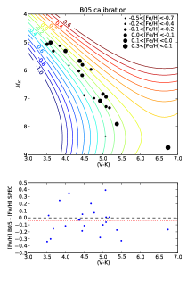
(a) B05 Calibration

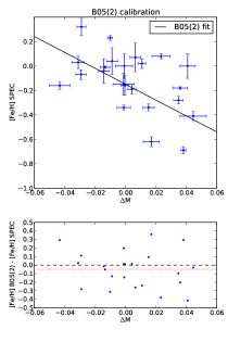
(b) B05(2) Calibration

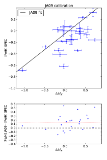
(c) JA09 Calibration

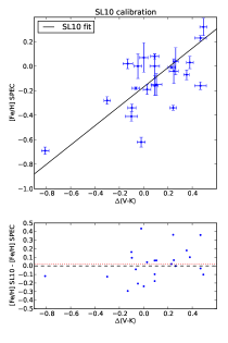
(d) SL10 Calibration

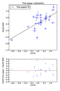
(e) This paper

Figure 1: The different [Fe/H] calibrations from Bonfils et al. (2005) (a and b), Johnson & Apps (2009) (c), Schlaufman & Laughlin (2010) (d), and the calibration determined in this paper (e). In each upper panel, the blue/black dots represent the data points. The black line depicts a fit to the data except in panel (a), where the calibrated [Fe/H] is shown as isometallicity contours. The lower subpanels show the difference between the calibrated and the spectroscopic metallicity. The black dashed lines represent the null value, and the red dotted line represents the mean difference for that calibration.

Table 4: Spectroscopic metallicity of the primaries and metallicities predicted for the secondary by the different calibrations.

Primary	Secondary	[Fe/H] [dex]
		Spectroscopic	B05	B05(2)	JA09	SL10	This paper
Gl53.1A	Gl53.1B	0.07	-0.21	-0.19	-0.05	-0.17	-0.17
Gl56.3A	Gl56.3B	0.00	-0.34	-0.42	-0.07	-0.21	-0.20
Gl81.1A	Gl81.1B	0.08	-0.22	-0.30	0.02	-0.10	-0.12
Gl100A	Gl100C	-0.28	-0.39	-0.38	-0.31	-0.41	-0.34
Gl105A	Gl105B	-0.19	-0.18	-0.18	-0.03	-0.15	-0.15
Gl140.1A	Gl140.1B	-0.41	-0.38	-0.44	-0.12	-0.25	-0.23
Gl157A	Gl157B	-0.16	0.04	0.13	0.36	0.20	0.10
Gl173.1A	Gl173.1B	-0.34	-0.27	-0.25	-0.14	-0.25	-0.23
Gl211	Gl212	0.04	-0.08	-0.09	0.15	0.04	-0.02
Gl231.1A	Gl231.1B	-0.01	-0.11	-0.06	0.15	0.01	-0.04
Gl250A	Gl250B	-0.15	-0.18	-0.14	0.04	-0.09	-0.11
Gl297.2A	Gl297.2B	0.03	0.00	0.05	0.27	0.13	0.05
Gl324A	Gl324B	0.32	-0.01	0.04	0.34	0.22	0.11
Gl559A	Gl551	0.23	0.06	-0.08	0.19	0.20	0.10
Gl611A	Gl611B	-0.69	-0.30	-0.40	-0.64	-0.81	-0.64
Gl653	Gl654	-0.62	-0.27	-0.26	-0.07	-0.19	-0.18
Gl666A	Gl666B	-0.34	-0.09	-0.14	0.12	0.02	-0.03
Gl783.2A	Gl783.2B	-0.16	-0.15	-0.15	0.02	-0.10	-0.12
Gl797A	Gl797B	-0.07	-0.02	0.04	0.25	0.11	0.03
GJ3091A	GJ3092B	0.02	-0.15	-0.22	-0.15	-0.27	-0.25
GJ3194A	GJ3195B	0.00	-0.19	-0.14	0.04	-0.10	-0.12
GJ3627A	GJ3628B	-0.04	-0.10	-0.06	0.16	0.03	-0.03
NLTT34353	NLTT34357	-0.18	-0.34	-0.38	-0.10	-0.22	-0.21

4 The latest metallicity measurements and calibrations

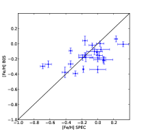
(a) B05 Calibration

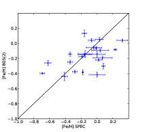
(b) B05(2) Calibration

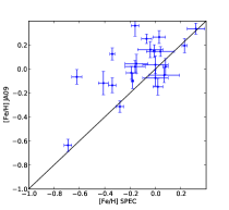
(c) JA09 Calibration

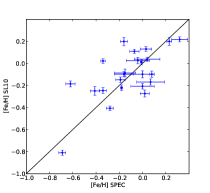
(d) SL10 Calibration

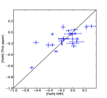
(e) This paper

Figure 2: [Fe/H] estimated from the the calibrations versus spectroscopic metallicity.The blue dots with error bars represent the data points. The black line depicts a one-to-one relationship.

In this section we discuss the three photometric metallicity calibrations in turn, and examine their agreement with our spectroscopic sample. Figure 2 plots the [Fe/H] obtained from each calibration against the spectroscopic [Fe/H], and it guides us through that discussion.

4.1 Bonfils et al. (2005) calibration

As recalled in the introduction, B05 first calibrated position in a $\{(V-K_{s})-M_{K_{s}}\}$ color-magnitude diagram into a useful metallicity indicator. That calibration is anchored, on the one hand, in spectroscopic metallicity measurements of early metal-poor M-dwarfs by Woolf & Wallerstein (2005), and on the other hand, in later and more metal-rich M dwarfs which belong in multiple systems for which B05 measured the metallicity of a hotter component. The B05 calibration has a $\sim$0.2 dex dispersion. Then, they used the calibration to measure the metallicity distribution of a volume-limited sample of 47 M dwarfs, which they found to be more metal-poor (by 0.07 dex) than 1000 FGK stars, with a modest significance of 2.6 $\sigma$. As mentioned above, Bonfils et al. (2007) used that calibration to compare M dwarfs with and without planets, and found that planet hosts are marginally metal-rich.

For our sample, the B05 calibration is offset by $-0.04\pm 0.04$ dex and has a dispersion of 0.20$\pm$0.02 dex. The negative offset is in line with SL10 finding (see Section 4.3) that B05 generally underestimates the true [Fe/H]. Correcting from this $-0.04$ offset almost eliminates the metallicity difference between local M dwarfs and FGK stars.

SL10 also report that the B05 calibration has a very poor $R^{2}_{ap}$, under 0.05, and that their own model explains almost an order of magnitude more of the variance of their calibration sample. In Sect. 3, we noted, however, that $R^{2}_{ap}$ is a noisy diagnostic for small samples.

In addition to their more commonly used calibration, B05 provide an alternative formulation for [Fe/H]. That second expression, labeled B05(2) in Table 3, works from the difference between the $V$- and $K_{s}$-band mass-luminosity relations of Delfosse et al. (2000). The two B05 formulations perform essentially equally for our sample, with B05(2) having a marginally higher dispersion. In the remainder of this paper we therefore no longer discuss B05(2).

4.2 Johnson & Apps (2009) calibration

Johnson & Apps (2009) argue that local M and FGK dwarfs should have the same metallicity distribution, and accordingly chose to fix their mean M dwarf metallicity to the value ($-0.05$ dex) for a volume-limited sample of FGK dwarfs from the Valenti & Fischer (2005) sample. They defined a sequence representative of average M dwarfs in the $\{(V-K_{s})-M_{K_{s}}\}$ color-magnitude diagram, and used the distance to that main sequence along $M_{K_{s}}$ as a metallicity diagnostic. They note that the inhomogeneous calibration sample of B05 is a potential source of systematics, and consequently chose to calibrate their scale from the metallicities of just six metal-rich M dwarfs in multiple systems with FGK primary components.

JA09 present two observational arguments for fixing the mean M dwarf metallicity. They first measured [Fe/H] for 109 G0-K2 stars (4900$<$T_eff$<$5900 K) and found no significant metallicity gradient over this temperature range, from which they conclude that no difference is to be expected for the cooler M dwarfs. We note, however, that a linear fit to their G0-K2 data set ([Fe/H]= $9.74\times 10^{-5}(T_{\rm eff}-5777)-0.04$) allows for a wide metallicity range when extrapolated to the cooler M dwarfs (2700$<$Teff$<$3750, for M7 to M0 spectral type, with [Fe/H] $=-0.24$ allowed at the 1 $\sigma$ level for an M0 dwarf and significantly lower than the [Fe/H] offset in B05. More importantly, they measured a large (0.32 dex) offset between the B05 metallicities of six metal-rich M dwarfs in multiple systems and the spectroscopic metallicities which they measured for their primaries. This robustly points to a systematic offset in the B05 calibration for metal-rich M dwarfs, but does not directly probe the rest of the (T_eff, [Fe/H]) space. We do find that the JA09 calibration is a good metallicity predictor for our sample at high metallicities, where its calibrator was chosen. With decreasing metallicity, that calibration increasingly overestimates the metallicity, however, as previously pointed out by SL10 (see below). Quantitatively, we measure a $+0.14\pm 0.04$ dex offset for our sample and a dispersion of $0.24\pm 0.04$.

4.3 Schlaufman & Laughlin (2010) calibration

Schlaufman & Laughlin (2010) improve upon B05 and JA09 in two ways. They first point out that, for M and FGK dwarfs to share the same mean metallicity, matched kinematics is as important as volume completeness. Since the various kinematic populations of our Galaxy have very different mean metallicities, the mean metallicity of small samples fluctuates very significantly with their small number of stars from the metal-poor populations. To overcome this statistical noise, they draw from the Geneva-Copenhagen Survey volume-limited sample of F and G stars a subsample that kinematically matches the volume limited sample of M dwarfs used by JA09. They find a $\simeq-0.14\pm 0.06$ dex mean metallicity for that sample, $0.09$ dex lower than adopted by JA09. However, they only used that sample to verify that the mean metallicity of M dwarfs in the solar neighborhood is well defined. In the end, the M dwarfs within a sample of binaries with an FGK primary that they used to fix their calibration are not volume-limited or kinematically-matched, but their mean metallicity ([Fe/H] = $-0.17\pm 0.07$) is statistically indistinguishable from the mean metallicity of the volume-limited and kinematically-matched sample.

Second, they use stellar evolution models to guide their parametrization of the color-magnitude space. Using [Fe/H] isocontours for the Baraffe et al. (1998) models, they show that in a {$(V-K_{s})-M_{K_{s}}$} diagram, changing [Fe/H] affects ($V-K_{s}$) at an essentially constant $M_{K_{s}}$. The metallicity is therefore best parametrized by ($V-K_{s}$), and their calibration uses a linear function of the ($V-K_{s}$) distance from a nominal sequence in the {$(V-K_{s})-M_{K_{s}}$} diagram. They do not force any specific mean metallicity, but verify a posteriori that it matches expectations.

We measure a $0.14\pm 0.02$ dex dispersion for the SL10 sample against their calibration, but that calibration has a significantly higher dispersion of $0.19\pm 0.03$ for our validation sample. That increased dispersion reflects our sample probing a wider metallicity range than SL10, as verified by computing the dispersion of an 18 star subsample that matches the metallicity range of the SL10 sample. That dispersion is $0.15\pm 0.03$ dex, and indistinguishable from $0.14\pm 0.02$ dex for the SL10 sample. The increased dispersion for a wider metallicity range suggests that a linear function of ($V-K_{s}$) does not fully describe metallicity. We also measure an offset of $0.02\pm 0.04$ dex. Offset and rms both improve over either of the B05 and JA10 calibrations.

4.4 Refining the Schlaufman & Laughlin (2010) calibration

We produced updated coefficients for the SL10 prescription, using the $RMS_{p}$ free parameter $p=2$ (see Sect. 3). The expression for the new metallicity calibration is

$$[Fe/H]=0.57\Delta(V-K_{s})-0.17,$$ (3)

$$\indent\Delta(V-K_{s})=(V-K_{s})_{obs}-(V-K_{s})_{iso},$$

where $(V-K_{s})_{obs}$ is the observed $V-K_{s}$ color and $(V-K_{s})_{iso}$ is a fifth-order polynomial function of $M_{K_{s}}$ that describes the mean main sequence of the solar neighborhood from the Valenti & Fischer (2005) catalog. This expression is adopted from Schlaufman & Laughlin (2010), who adapted an $M_{K_{s}}$ vs $(V-K_{s})$ formula from Johnson & Apps (2009).

Table 3 shows limited differences between this new fit and the original SL10 calibration. The dispersion of the new fit is tighter by just 0.02 dex ($0.17\pm 0.03$ dex instead of $0.19\pm 0.03$), and the offset is now $0.00\pm 0.04$, as expected. The R${}^{2}_{ap}$ value is similar ($0.43\pm 0.23$ vs $0.41\pm 0.29$) and uncertain. Readjusting the coefficients therefore produces a marginal improvement at best.

The dispersion, in all panels of Fig. 1, is well above the measurement uncertainties. Those therefore contribute negligibly to the overall dispersion, which must be dominated by other sources.

As can be seen in Fig. 2, B05 or B05(2) tend to underestimate [Fe/H], while the JA09 calibration clearly overestimates [Fe/H] except at the highest metallicities.

5 Summary

We have assembled a sample of M dwarf companions to hotter FGK stars, where the system has an accurate parallax and the M dwarf component has accurate $V$ and $K_{s}$-band photometry. Using the metallicities of the primaries, newly measured or retrieved from the literature, and the assumption that the two components have identical initial compositions, we compared the dispersions of the Bonfils et al. (2005), Johnson & Apps (2009), and Schlaufman & Laughlin (2010) photometric metallicity calibrations. We find that the Schlaufman & Laughlin (2010) scale, which is intermediate between Bonfils et al. (2005) and Johnson & Apps (2009), has the lowest dispersion. We slightly refine that relation, by readjusting its coefficients on our sample.

We find that our tight selection of binaries with accurate parallaxes and photometry sample has insignificantly reduced the dispersion of the measurements around the calibration compared to looser criteria. This suggests that the dispersion, hence the random errors of the calibration, is not defined by measurement uncertainties but instead reflects intrinsic astrophysical dispersion. Nonlinearities in the metallicity dependence of the $V-K_{s}$ color are likely to contribute, as suggested both by atmospheric models (Allard, private communication) and by the increased dispersion that we measure over a wider metallicity range. They are, however, unlikely to be the sole explanation, since we see dispersion even in narrow areas of the color-magnitude diagram. Stellar evolution cannot significantly contribute, since early-M dwarfs evolve rapidly to the main sequence and they remain there for much longer than a Hubble time, but rotation and magnetic activity could play a role. Unless, or until, we develop a quantitative understanding of this astrophysical dispersion, the photometric calibration approach may therefore have reached an intrinsic limit. Those calibrations also have the very practical inconvenience of needing an accurate parallax. This limits their use to the close solar neighborhood, at least until the GAIA catalog becomes available in a decade.

Alternative probes of the metallicities of M dwarfs are therefore obviously desirable. One obvious avenue is to work from higher spectral resolution information and to identify spectral elements that are most sensitive to metallicity and others that are most sensitive to effective temperature. We are pursuing this approach at visible wavelengths (Neves et al. in prep.), as do Rojas-Ayala et al. (2010, see Appendix A.2) in the near infrared, with encouraging results in both cases.

Appendix A Other methods

A.1 Calibration of Casagrande et al. (2008)

In Sect. 4 we described the photometric metallicity calibrations in detail. Casagrande et al. (2008) devised a completely different technique, based on their previous study of FGK stars using the infrared flux method (Casagrande et al. 2006), to determine effective temperatures and metallicities. The infrared flux method uses multiple photometry bands to derive effective temperatures, bolometric luminosities, and angular diameters. The basic idea of IRFM (Blackwell & Shallis 1977) is to compare the ratio between the bolometric flux and the infrared monochromatic flux, both measured on Earth, to the ratio between the surface bolometric flux ($\propto\sigma Teff^{4}$) and the surface infrared monochromatic flux for a model of the star. To adapt this method to M dwarfs, Casagrande et al. (2008) added optical bands, creating the so-called MOITE, Multiple Optical and Infrared TEchnique. This method provides sensitive indicators of both temperature and metallicity. The proposed effective temperature scale extends down to 2100-2200 K, into the L-dwarf limit, and is supported by interferometric angular diameters above $\sim$ 3000K. Casagrande et al. (2008) obtain metallicities by computing the effective temperature of the star for each color band $(V(RI)_{c}JHK_{s})$ for several trial metallicities, between $-$2.1 and 0.4 in 0.1 dex steps, and by selecting the metallicity that minimizes the scatter among the six trial effective temperatures. Casagrande et al. (2008) estimate that their total metallicity uncertainty is 0.2 to 0.3 dex.

Table 5: Metallicity values from spectroscopy and obtained using the method of Casagrande et al. (2008) (C08 in this table).

Primary	Secondary	[Fe/H] [dex]
		Spectroscopic	C08
Gl53.1A	Gl53.1B	0.07	-0.07
Gl56.3A	Gl56.3B	0.00	-0.21
Gl81.1A	Gl81.1B	0.08	-0.08
Gl100A	Gl100C	-0.28	-0.10
Gl105A	Gl105B	-0.19	-0.30
Gl140.1A	Gl140.1B	-0.41	-0.30
Gl157A	Gl157B	-0.16	-0.10
Gl173.1A	Gl173.1B	-0.34	-0.20
Gl211	Gl212	0.04	-0.21
Gl231.1A	Gl231.1B	-0.01	-0.28
Gl250A	Gl250B	-0.15	-
Gl297.2A	Gl297.2B	0.03	0.00
Gl324A	Gl324B	0.32	-0.20
Gl559A	Gl551	0.23	-
Gl611A	Gl611B	-0.69	-0.40
Gl653	Gl654	-0.62	-0.30
Gl666A	Gl666B	-0.34	-
Gl783.2A	Gl783.2B	-0.16	-0.30
Gl797A	Gl797B	-0.07	-0.90
GJ3091A	GJ3092B	0.02	-0.30
GJ3194A	GJ3195B	0.00	-0.60
GJ3627A	GJ3628B	-0.04	-0.20
NLTT34353	NLTT34357	-0.18	0.19

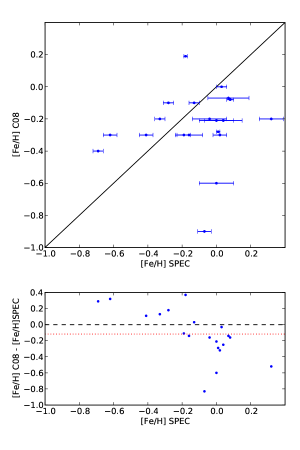
Figure 3: [Fe/H] obtained with the Casagrande et al. (2008) method versus the spectroscopic metallicity. The blue dots with error bars represent the data points. The black line depicts a one-to-one relationship. The metallicity difference between the values of the calibrations and the spectroscopic measurements is shown below each [Fe/H]-[Fe/H] plot. The black dashed line is the zero point of the difference, and the red dotted line represents the average of the metallicity difference.

The MOITE method does not reduce into a closed form that can be readily applied by others, but Luca Casagrande kindly computed MOITE [Fe/H] values for our sample (Table 5). We evaluated the calibration in the same manner as in Sect. 3 and obtained a value of $-0.11\pm 0.07$ dex for the offset, $0.32\pm 0.06$ dex for the rms, $0.10\pm 0.04$ dex for the RMS_P, and $-1.09\pm 1.45$ for the R${}^{2}_{ap}$. From these values and from Fig. 3, we can observe that the Casagrande et al. (2008) calibration has a higher rms and RMS_p and a poorer R${}^{2}_{ap}$ than the three photometric calibrations, consistently with the high metallicity uncertainty referred by Casagrande et al. (2008). The negative R${}^{2}_{ap}$ value formally means that this model increases the variance over a constant metallicity model, but as usual R${}^{2}_{ap}$ is a noisy diagnostic.

A.2 Rojas-Ayala et al. (2010) calibration

Rojas-Ayala et al. (2010) have recently published a novel and potentially very precise technique for measuring M dwarf metallicities. Their technique is based on spectral indices measured from moderate-dispersion ($R\sim 2700$) $K$-band spectra, and it needs neither a $V$ magnitude nor a parallax, allowing measurement of fainter (or/and farther) stars. They analyzed 17 M dwarf secondaries with an FGK primary, which also served as metallicity calibrators, and measured the equivalent widths of the NaI doublet (2.206 and 2.209 $\mu m$), and the CaI triplet (2.261, 2.263 and 2.265 $\mu m$). With these measurements and a water absorption spectral index sensitive to stellar temperatures, they constructed a metallicity scale with an adjusted multiple correlation coefficient greater than the one of Schlaufman & Laughlin (2010) ($R^{2}_{ap}=0.63$), and also with a tighter RMS_p of 0.02 when compared to other studies (0.05, 0.04, and 0.02 for Bonfils et al. 2005, Johnson & Apps 2009, and Schlaufman & Laughlin 2010 respectively). The metallicity calibration is valid over -0.5 to +0.5 dex, with an estimated uncertainty of $\pm$0.15 dex.

A test of the Rojas-Ayala et al. (2010) calibration for our full sample would be very interesting, but is not currently possible for lack of near-infrared spectra for most of the stars. Seven of our stars, however, have their metallicities measured in Rojas-Ayala et al. (2010) (Gl 212, Gl 231.1B, Gl 250B, Gl 324B, Gl611B, Gl783.2B, and Gl 797B with predicted [Fe/H] of $0.09,-0.05,-0.04,0.30,-0.49,-0.19$, and $-0.06$ dex, respectively). We find a dispersion of only 0.08 dex and an offset of 0.04 dex offset between our spectroscopic measurements of the primaries and the Rojas-Ayala et al. (2010) metallicities of the secondaries. These numbers are extremely encouraging, but still have little statistical significance. They will need to be bolstered by testing against a larger sample and over a wider range of both metallicity and effective temperature.