Hubbard-I approach to the Mott transition

Abstract

We expose the relevance of double occupancy conservation symmetry in application of the Hubbard-I approach to strongly correlated electron systems. We propose the utility of a composite method, viz. the Hubbard-I method in conjunction with strong coupling perturbation expansion, for studying systems violating the afore–mentioned symmetry. We support this novel approach by presenting a first successful Hubbard-I type calculation for the description of the metal-insulator Mott transition in a strongly correlated electron system with conserved double occupancies, which is a constrained Hubbard Hamiltonian equivalent to the Hubbard bond charge Hamiltonian with $X=t$. In particular, we obtain the phase diagram of this system for arbitrary fillings, including details of the Mott transition at half-filling. We also compare the Hubbard-I band–splitting Mott transition description with results obtained using the standard Gutzwiller Approximation (GA), and show that the two approximate approaches lead to qualitatively different results. In contrast to the GA applied to the system studied here, the Hubbard-I approach compares favourably with known exact results for the $d=1$ dimensional chain.

I Introduction

The metal to Mott insulator (MI) transition, envisaged by Mott Mott , is one of the striking effects induced by strong electronic correlations in many electron systems. The Coulomb interaction between electrons $U$ leads to highly correlated ground states in these systems, rendering their description quite challenging. As a result there have been various theoretical attempts at providing a satisfying description of the Mott transition.

The first of these was due to Hubbard HubbardI , who provided a seminal nonperturbative approach – the so-called Hubbard-I (H-I) approximation – to a simplified interacting electron problem described by the Hubbard model. H-I describes both (i) the atomic limit (i.e. limit of vanishing bandwidth $W\rightarrow 0$) exactly, in particular yielding two atomic levels corresponding to single and double local occupancy, and (ii) the non-interacting case ($U=0$) exactly, and so held some promise of describing the intermediate physics in a consistent interpolating fashion. For finite bandwidth, the atomic levels broaden into two “dynamic” (sub)bands which are occupation-number and interaction dependent. These are always split by a gap for all $U>0$ indicating an insulator phase. Unfortunately H-I approach in relation to the Hubbard model is flawed at a basic level. (i) It is not a particle-hole symmetry conserving approximation HubbardI (it is not guaranteed that the Mott insulator phase exists only exactly at half-filling). (ii) Hubbard-I predicts a Mott transition at $U=0$, which certainly is not true in general - the Hubbard model on the honeycomb lattice e.g. has a finite critical point $U_{c}$ Paiva2005 . More importantly, the Hubbard-I does not yield a viable description of the weak coupling limit $U/W\ll 1$, in particular it does not reproduce the renormalized Fermi liquid expected from the Hartree-Fock approximation. The situation was somewhat improved in the Hubbard-III approximation HubbardIII , where scattering and resonance broadening corrections shift the transition point to $U_{c}\sim W$. However, this approach does not predict the expected Fermi liquid properties on the metallic side, Edwards . The Hubbard approaches were very important for the conceptual introduction of the Hubbard subbands, however their problems have led some autors to the rejection of Hubbard approximations for the study of strongly correlated electron systems. In spite of these issues, however, as shown in a recent study by Dorneich et al. Dorneich2000 , a suitably generalized Hubbard-I approach actually gives reasonably good description even at the quantitative level in the limit of strong interaction (large $U$) and weak spin correlations, of the Hubbard model.

A complementary approach, starting from the weak coupling limit, is based on the Gutzwiller variational wave function Gutzwiller (GWF), which describes an increasingly correlated Fermi liquid with increasing interaction $U$. Brinkman and Rice Rice showed, using the so-called Gutzwiller approximation Gutzwiller (GA), that increase in $U$ is associated with the diminishing of the quasiparticle residue of the Fermi liquid, or equivalently with the increase in quasiparticle effective mass. In this framework, a metal-insulator transition occurs at finite value $U_{c}$ when the effective mass diverges and is thus driven by quasiparticle localisation. This method gives a good low energy description of the metal, but does not describe the precursors of the Hubbard bands which should plausibly appear on the metallic side. Importantly, for finite dimensional systems, the GBR transition is an artefact of the GA, since analytical Millis ; Dzierzawa and numerical studies Yokoyama of the GWF show that it always describes a metallic state.

Although, both these early methods have their flaws, they hint at two possible mechanisms behind the Mott transition. These two pictures have been brought to the forefront, more recently, with the development of more involved contemporary methods, in particular dynamical mean field theory (DMFT) Kotliar which provides a bridge between the formation of Hubbard bands on the one hand, and strongly correlated fermi liquid behaviour on the other. In particular, the DMFT inspired modern prevailing view is that quasiparticle localization drives the ground state Mott transition in the Hubbard model Kotliar .

In this paper, we reconsider the Hubbard-I type approach as a systematic means of obtaining a band-splitting theory of the Mott transition. Instead of trying to improve H-I approximation as a method for general strongly correlated Hamiltonians we rather seek to specify which Hamiltonians may be successfully studied by a standard H-I approximation. We shall argue that there are correlated Hamiltonians, viz. those describing electron systems with so-called extreme correlations Shastryex , for which the Hubbard-I approach provides a basic ”mean-field”–like description.

The paper is organized as follows: In Section 2 we discuss the relevance of double occupation conservation symmetry for the application of the H-I approximation. In Section 3 we consider the H-I approach to one of the simplest Hamiltonians preserving this symmetry as a model of a band-splitting theory of the Mott transition. In Section 4 we compare results with known features of the Hubbard bond-charge model - an equivalent model on bipartite lattices. Section 5 consists of a short discussion of corrections to the H-I approach for the studied Hamiltonian. Finally section 6 is devoted to a comparison of two complementary theories of the Mott transition: band-splitting driven and quasiparticle localisation driven.

II Inspection of the Hubbard-I approach

Contrary to early expectations, we now see the Hubbard approach, based on a Green’s function decoupling scheme, as a large–U approximation, despite its non perturbative nature. One may therefore suspect that some problems encountered in the Hubbard approach may originate in limitations of strong-coupling perturbation theory.

Consider therefore the Hubbard model: $H=\hat{T}+U\hat{D}$, where $\hat{D}=\sum_{i}n_{i\uparrow}n_{i\downarrow}$ is the number of doubly occupied sites and $\hat{T}=\sum_{i,j,\sigma}t_{i,j}c_{i\sigma}^{\dagger}c_{j\sigma}$ is the kinetic energy. The large-U perturbational expansion starts from splitting the kinetic energy into three parts $\hat{T}=\hat{T}_{0}+\hat{T}_{+1}+\hat{T}_{-1}$. $\hat{T}_{0}=\hat{T}_{UHB}+\hat{T}_{LHB}$ is the double occupancy conserving hopping (commuting perturbation) in the Upper and Lower Hubbard Bands:

$$\hat{T}_{UHB}=\sum_{i,j,\sigma}t_{ij}n_{i\bar{\sigma}}c_{i\sigma}^{\dagger}c_{j\sigma}n_{j\bar{\sigma}},$$

$$\hat{T}_{LHB}=\sum_{i,j,\sigma}t_{ij}(1-n_{i\bar{\sigma}})c_{i\sigma}^{\dagger}c_{j\sigma}(1-n_{j\bar{\sigma}}),$$

corresponding to hopping of projected electrons on doubly and singly occupied sites respectively. The remaining hopping terms $\hat{T}_{+1}$ and $\hat{T}_{-1}=\hat{T}_{+1}^{\dagger}$ correspond to interband hopping (non–commuting perturbation). The perturbational expansion for the Hubbard model is well known and can be performed e.g. using the method of canonical transformations HarrisLange ; Chao which to second order yields the effective Hamiltonian:

$$H^{(2)}_{\rm eff}=\hat{T}_{0}+U\hat{D}+\frac{1}{U}[\hat{T}_{+1},\hat{T}_{-1}].$$ (1)

Recall that the perturbation expansion to any order eliminates mixing between the degenerate subspaces of the unperturbed Hamiltonian $\hat{U}$ and leads to an effective Hamiltonian with emergent symmetry of conservation of the number of doubly occupied sites. Due to this property, the average of operators jointly changing the total number of doubly occupied sites, such as e.g. $\langle c_{j\sigma}n_{j\bar{\sigma}}c_{l\sigma}^{\dagger}h_{l\bar{\sigma}}\rangle$,($h_{j\bar{\sigma}}=1-n_{j\bar{\sigma}}$ is the on-site hole occupation number), are identically zero leading to the vanishing of the associated Green’s functions. Thus in this framework, the single particle Green’s function $G_{lj}^{\sigma}=\langle\langle c_{l\sigma}|c_{j\sigma}^{\dagger}\rangle\rangle$ decomposes into a sum of two Green’s functions $\Gamma_{lj}^{\sigma}=\langle\langle c_{l\sigma}n_{l\bar{\sigma}}|c_{j\sigma}^{\dagger}n_{j\bar{\sigma}}\rangle\rangle$ and $\widetilde{\Gamma}_{lj}^{\sigma}=\langle\langle c_{l\sigma}h_{l\bar{\sigma}}|c_{j\sigma}^{\dagger}h_{j\bar{\sigma}}\rangle\rangle$ related to the propagation of fermionic quasiparticles, in the upper and lower Hubbard bands respectively.

Interestingly the Hubbard-I approach is most naturally described by the separation of an electron into two non-canonical fermions $c_{j\sigma}=c_{j\sigma}n_{j\bar{\sigma}}+c_{j\sigma}h_{j\bar{\sigma}}$ HubbardIV . Consider therefore the H-I approach to the simplest non-trivial level of strong-coupling perturbational expansion, described by the first two terms in the expansion Eq.(1)

$$H_{c}=\hat{T}_{0}+U\hat{D}.$$ (2)

In the frequency domain, the equations of motion for the basic Green’s function are $\omega\Gamma_{lj}^{\sigma}(\omega)=\frac{1}{2\pi}\langle n_{l\bar{\sigma}}\rangle\delta_{lj}+\langle\langle[c_{l\sigma}n_{l\bar{\sigma}},H_{{\rm c}}]|c_{j\sigma}^{\dagger}n_{j\bar{\sigma}}\rangle\rangle_{\omega}$ and $\omega\widetilde{\Gamma}_{lj}^{\sigma}(\omega)=\frac{1}{2\pi}\langle h_{l\bar{\sigma}}\rangle\delta_{lj}+\langle\langle[c_{l\sigma}h_{l\bar{\sigma}},H_{{\rm c}}]|c_{j\sigma}^{\dagger}h_{j\bar{\sigma}}\rangle\rangle_{\omega}$. We perform the following mean-field or H-I type of decoupling on the higher order Green’s function in the equations for $\Gamma_{lj}^{\sigma}(\omega)$ to terminate the sequence of equations at the level of the upper and lower band Green’s functions:

$$\langle\langle c_{l+\delta\sigma}n_{l+\delta\bar{\sigma}}n_{l\bar{\sigma}}|c_{j\sigma}^{\dagger}n_{j\bar{\sigma}}\rangle\rangle_{\omega}\approx\langle n_{l\bar{\sigma}}\rangle\Gamma_{l+\delta,j}^{\sigma}(\omega)$$

$$\langle\langle c_{l\sigma}c_{l\bar{\sigma}}^{\dagger}c_{l+\delta\bar{\sigma}}n_{l+\delta\sigma}|c_{j\sigma}^{\dagger}n_{j\bar{\sigma}}\rangle\rangle_{\omega}\approx\langle c_{l\sigma}c_{l\bar{\sigma}}^{\dagger}\rangle\langle\langle c_{l+\delta\bar{\sigma}}n_{l+\delta\sigma}|c_{j\sigma}^{\dagger}n_{j\bar{\sigma}}\rangle\rangle_{\omega}$$

$$\langle\langle h_{l+\delta\sigma}c_{l+\delta\bar{\sigma}}^{\dagger}c_{l\bar{\sigma}}c_{l\sigma}|c_{j\sigma}^{\dagger}n_{j\bar{\sigma}}\rangle\rangle_{\omega}\approx\langle c_{l\bar{\sigma}}c_{l\sigma}\rangle\langle\langle c_{l+\delta\bar{\sigma}}^{\dagger}h_{l+\delta\sigma}|c_{j\sigma}^{\dagger}n_{j\bar{\sigma}}\rangle\rangle_{\omega}$$

with analogous complementary treatment of the set $\widetilde{\Gamma}_{lj}^{\sigma}(\omega)$. The last two decouplings lead to magnetic and superconducting order parameters and which are set here to zero, as we are interested in the description of a paramagnetic Mott transition. Solving the equations of motion, one obtains the following momentum (or Fourier transformed) Green’s functions for the system:

$$\Gamma_{\bm{k}}^{\sigma}(\omega)=\frac{1}{2\pi}\frac{n_{\bar{\sigma}}}{\omega-(n_{\bar{\sigma}}\epsilon_{\bm{k}}+U-\mu)}$$ (3)

$$\widetilde{\Gamma}_{\bm{k}}^{\sigma}(\omega)=\frac{1}{2\pi}\frac{1-n_{\bar{\sigma}}}{\omega-((1-n_{\bar{\sigma}})\epsilon_{\bm{k}}-\mu)}$$ (4)

The electron Green’s function $G_{\bm{k}}^{\sigma}(\omega)=\langle\langle c_{k\sigma}|c_{k\sigma}^{\dagger}\rangle\rangle_{\omega}=\Gamma_{\bm{k}}^{\sigma}(\omega)+\widetilde{\Gamma}_{\bm{k}}^{\sigma}(\omega)$ thus has the characteristic Hubbard-I two pole form describing two subbands, however the poles here have an elementary form in comparison with the solution for the full Hubbard model HubbardI . The main result stemming from these Green’s functions is that a Mott transition, identified with band separation, is elevated to finite interaction $U$. Indeed, for a paramagnetic configuration at half filling $\langle n_{\uparrow}\rangle=\langle n_{\uparrow}\rangle=1/2$ the lowest energy in the UHB is readily read out from Eq.(3) to be $U-W/4$, while the highest energy in the LHB is from Eq.(4) $W/4$ (where $W$ is the free electron bandwidth), hence a gap opens at a critical value $U_{c}=W/2$. Importantly, the presented solutions Eqs.(3,4) are explicitly electron hole symmetric. Accordingly, the gap opening at $U=W/2$ is associated with a Mott transition only exactly at half-filling.

These results provide explicit evidence that the source of problems in the Hubbard-I approach stem from the effects of the double occupancy non–conserving terms $T_{\pm 1}$. Since the Hubbard-I approach leads to the separation of an electron into two non-canonical fermions $c_{j\sigma}=c_{j\sigma}n_{j\bar{\sigma}}+c_{j\sigma}h_{j\bar{\sigma}}$ which are subsequently treated separately, we view the source problem as that of incompatibility of the one band electron normal Landau-Fermi liquid (consistent with the full hopping operator $\hat{T}$) with the two (bands of) non-canonical fermion liquids (consistent with double occupancy number conservation). In fact, the two non-canonical liquids cannot be adiabatically connected to the normal Fermi liquid, so one should rather consider the Hubbard-I as a mean-field type approach appropriate for systems conserving double occupancies, such as those obtained in strong coupling perturbational theory at any order, not arbitrary systems. We defer discussion of our Hubbard-I approach to other and higher order Hamiltonians to later papers, and in the remainder of this paper we shall analyze results for the model in Eq.(2).

III The Mott transition

The constrained Hamiltonian $H_{c}$ Eq.(2) is interesting in itself because it can be viewed as a particular model of extremely correlated electrons. Recall that the term extremely correlated electron systems has recently been introduced by Shastry Shastryex , emphasizing the appearance of noncanonical fermions resulting from the prohibition of double occupancies in the $U=\infty$ limit, which is a special case of symmetry of conserved double occupancies. The model $H_{c}$ considered here, that allows for double occupancies which are conserved and thus describes hopping of noncanonical (constrained) fermions $c_{j\sigma}n_{j\bar{\sigma}}$ and $c_{j\sigma}h_{j\bar{\sigma}}$ can therefore be considered a generalization of the problem of extremely correlated fermions for general interaction strength $U$. Note that the model $H_{c}$ contains the $U\rightarrow\infty$ limit of the Hubbard model due to its perturbative origin. Even for small $U$ and low fillings, we discuss below that the ground states of $H_{c}$ correspond to the ground states of the $U=\infty$ Hubbard model.

We now consider the details of the Hubbard-I description of the zero temperature Mott transition in the model $H_{c}$ of extremely correlated electrons, as it is a first successful theory of a band-splitting driven Mott transition. The analysis is carried out only for the paramagnetic phases, with $n_{\uparrow}=n_{\downarrow}$.

From the band structure of the one particle Green’s function, it is evident that the insulator phase exists only if $U>U_{c}$ and the lower band is completely filled while the upper band is empty. The Green’s functions Eqs.(3,4) lead to the following equation for the number of electrons of a given spin species:

$$n_{\sigma}=(1-n_{\bar{\sigma}})\int_{-W/2}^{W/2}\!f((1-n_{\bar{\sigma}})\epsilon-\mu)\rho(\epsilon)\,\mathrm{d}\epsilon$$

$$+n_{\bar{\sigma}}\int_{-W/2}^{W/2}\!f(n_{\bar{\sigma}}\epsilon+U-\mu)\rho(\epsilon)\,\mathrm{d}\epsilon$$ (5)

where $f(\ldots)$ is the Fermi-Dirac distribution and $\rho(\epsilon)$ is the density of states. The boundaries of the insulator phase are obtained, independently of the lattice, when either $\mu=(1-n_{\bar{\sigma}})W/2$ is at the end of the lower band or $\mu=-n_{\bar{\sigma}}W/2+U$ is at the beginning of the upper band. For both these cases, at zero temperature, Eq.(5) reduces to $n_{\sigma}=1-n_{\bar{\sigma}}$, showing that the transition only occurs at half-filling, as claimed. The jump in $\mu$ at half-filling $n_{\uparrow}=n_{\downarrow}=1/2$ reduces to zero at $U=W/2$ indicating the transition point. The Mott “lobe” is shown in Fig.1. Note that the kinetic energy and interaction energy are both zero in the Mott phase, which is an exact feature of the model. Indeed, note that there is extensive degeneracy of localized Mott states consisting of one particle per site which are all exact ground states of the considered model (Eq.(2)), with zero kinetic energy due to double occupancy conservation.

Figure 1: Ground state phase diagram of the model $H_{c}$ in the $U-n$ plane. In all calculations we assume only nearest neighbour hopping $t_{ij}=-t$. A metallic ECFL exists for all $n\leq 1$. At low filling, the metal resembles the $U=\infty$ metallic phase of the Hubbard model, with no double occupancies. Closer to $n=1$, the metal has double occupancies and is described by two Fermi liquids per spin species. In the H-I calculation, the boundary between these two behaviours is a Lifshitz-type transition, shown for hyper-cubic lattices in 1,2,3 dimensions and for the rectangular DOS. Shown is also the exact result for 1d, from Ovchinnikov with rescaled $U\rightarrow U/2$, for comparison. All transition lines cross the $n=1$ line at finite $U=W/2$ marking the point of Mott transition. Solid line depicts the Mott phase. The $n>1$ can be obtained by invoking electron-hole symmetry. Inset: Ground state phase diagram in the $U-\mu$ plane. The electron hole symmetry line (dotted) separates $n<1$ and $n>1$ cases. The $n=1$ case coincides with this line for $U<W/2$ whereas for $U>W/2$ opens into a Mott insulator ”lobe” of finite width.

Outside the Mott phase, the system is in a metallic phase described, in the used approximation, by four (two per spin species) dispersion-less extremely correlated Fermi liquids (ECFLs) associated with the lower and upper Hubbard bands Eq.(3,4). Depending on the filling factor and value of $U$, for each spin species one can obtain a situation where only one kind of Fermi liquid of $c_{j\sigma}h_{j\bar{\sigma}}$ fermions appears, to which there pertains a single well defined Fermi surface (see Fig. 1). For $n<1$, this case is physically equivalent to the infinite $U$ limit of the Hubbard model. The single Fermi liquid comes about because for small $n_{\uparrow},n_{\downarrow}$ the lower Hubbard band is wide while the upper Hubbard band is very narrow. Even for $U<W/2$, although the two bands overlap, the upper band centered around $U$ is too narrow to be occupied in the ground state. On the other hand, closer to half filling $n\leq 1$ for $U<W/2$ when the upper band can also be occupied, two coexistent Fermi liquids of $c_{j\sigma}h_{j\bar{\sigma}}$ and $c_{j\sigma}n_{j\bar{\sigma}}$ fermions emerge, per spin species, associated with two Fermi surfaces. The boundary between these two cases is therefore a Fermi surface topology changing transition, which can be called a Lifshitz type transition.

The above band picture comes with a caveat, viz. the bands Eq.(3,4) which seem to be apparently independent in the Grand Canonical Ensemble (GCE) cannot be treated as such when attempting to construct arbitrary excitations. For constructing elementary excitations, at the very least an additional rule must be implemented to obtain physically relevant states, i.e. the upper bands pertaining to both spin indices must be equally populated (these are equal to the double occupancy) while the number of holes in the lower bands must also be equal. This may be seen as a type of “statistical interaction” Haldane ; Gebhard between the bands in this system. In the GCE, this problem is masked and taken care of, by the common value of the chemical potential for both species which guarantees equal population of the upper band and equal number of holes in the lower band, in the thermodynamic limit.

We now focus on the interaction driven Mott transition from the metallic phase. Unlike in the Gutwziller method, the hopping in the approach discussed here cannot be used as an indicator of the transition, as it remains constant. The density of doubly occupied sites $D=\langle\hat{D}\rangle/N$ (occupation of the upper Hubbard band) is a good parameter at half filling capturing the transition for this model. Using the Green’s function of Eq.(3) (or the second term in Eq.(5)) and the half-filling condition $\mu=U/2$, one obtains the particularly simple form at zero temperature

$$D=\langle\hat{D}\rangle/N=\frac{1}{2}\int_{-W/2}^{-U}\!\rho(\epsilon)\,\mathrm{d}\epsilon$$ (6)

which depends only on $U$ and the density of states. We show results for a few different density of states (DOSes) in Fig.2.

Note that an important feature of our Hubbard-I calculation is that the critical point does not depend on the lattice type. Furthermore, lattice dependent properties emerge for the number of doubly occupied sites. A linear dependence is associated here only with a rectangular density of states. In fact, the critical behaviour of $D$ has universal properties depending only on spatial dimensions of the lattice. It is governed by the behaviour of the DOS at the bottom of the band. Indeed for parabolic energy dispersions near the bottom of the band, as ${\epsilon}\rightarrow-W/2\Rightarrow\Delta\epsilon_{\bm{k}}\propto{\bm{k}}^{2}$, we have for 1 dimension $\rho(-W/2+\Delta\epsilon)\propto 1/\sqrt{\Delta\epsilon}$, 2 dimensions that $\rho(-W/2+\Delta\epsilon)\propto\mathrm{const.}$, and 3 dimensions $\rho(-W/2+\Delta\epsilon)\propto\sqrt{\Delta\epsilon}$. Then we obtain that in 1d: $D\propto[(U_{c}-U)/{U_{c}}]^{\frac{1}{2}}$ , 2d: $D\propto(U_{c}-U)/{U_{c}}$ while in 3d: $D\propto[(U_{c}-U)/{U_{c}}]^{\frac{3}{2}}$.

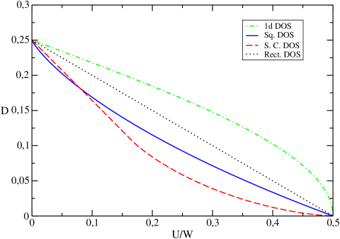
Figure 2: The double occupancy per site $D$ at half-filling $n=1$ as a function of $U$. Shown are results for hyper-cubic lattices in 1, 2, 3 dimensions and for rectangular DOS. For all DOSes $D=1/4$, at $U=0$, as in the uncorrelated metal, although it is a ECFL here. The Mott transition takes place at $U=W/2$. Note different critical behavior in 1,2 and 3 $d$. The curve calculated for 1$d$ coincides with known exact result Ovchinnikov for rescaled $U\rightarrow U/2$.

IV Relation to the Bond-charge Hubbard model

While the results presented in the previous paragraph provide a clear and simple quantitative picture of a paramagnetic transition as well as the metallic phase, one may wonder if the constrained model $H_{c}$ is realistic, as it was derived as lowest order of strong-coupling expansion. Additionally, it is not a priori clear how good an approximation the Hubbard-I approach yields for the constrained model $H_{c}$. Therefore it is important to note that this model is related to the class of generalized Hubbard models, differing from the Hubbard Hamiltonian by an additional bond charge interaction term (see e.g.:

$$H_{\rm bond-charge}=\hat{T}+U\hat{D}+\sum_{i,j,\sigma}X_{ij}(n_{i\bar{\sigma}}+n_{j\bar{\sigma}})c_{i\sigma}^{\dagger}c_{j\sigma}$$ (7)

which was already discussed by Hubbard HubbardI and reconsidered in relation to superconductivity by Micnas ; Hirsch ). Interestingly this is one of the few models in which there is a Mott transition in the ground state, for certain values of parameters Strack .

Indeed, at a symmetry point, when the bond charge interaction is equal to the hopping $X_{ij}=-t_{ij}$, this generalized Hubbard model conserves the number of double occupancies. In fact, the resultant symmetric model can be mapped onto the model $H_{c}$ on bipartite lattices, via the canonical transformation $U=\exp[-i\pi\sum_{j}{\bm{R}}_{j}n_{j\uparrow}n_{j\downarrow}]$, where $R_{j}=\pm 1$ on different sublattices, as shown in Gebhard . Analytical ground states of the symmetric bond-charge model were obtained in Strack in the regime $U>2W$ at half filling, for arbitrary dimensions $d$. These results were improved upon in Ovchinnikov revealing that a metal-insulator transition occurs at $U=W$, probably with ferromagnetic polarization on the metallic side (for $d>1$), which is supported by numerical evidence Gagliano .

The special case of $d=1$, was exactly solved in Ovchinnikov leading to the following main results: the metal to insulator transition occurs at $U_{c}=W$, and also the number of double occupancies is $D=1/2\pi{\rm ArcCos}(U/U_{c})$. In $d=1$, the H-I approach used here grossly underestimates the transition point, but remarkably the average number of double occupancies calculated for the 1-d DOS $\rho(\epsilon)=1/(\pi\sqrt{1-\epsilon^{2}})$, using Eq.(6) leads to exactly the same function and prefactor as the exact solution (with $U_{c}=W/2$ now being the H-I critical value). Interestingly, the exact results can also be interpreted in terms of lower and upper Hubbard bands, as shown in Gebhard . These bands however do not carry spin indices and the hopping is not renormalized, while also a different mechanism of statistical interaction than the one obtained here is present.

Furthermore, exact results away from half-filling $n=1$ reveal, that there is a critical boundary separating states with doubly occupied sites from states with no such sites, which in the H-I framework considered here corresponds to the Lishitz lines $U_{L}$ depicted in Fig.1. The exact boundary is given by the relation $U_{L}=W\cos(\pi(1-n))$ Ovchinnikov . Notice that, apart from the value of the Mott transition point, the Lifshitz line obtained using the H-I approach here is in good quantitative agreement with these results (see Fig.1). In general dimensions, the expected phase diagram is expected to be qualitatively similar Schadschneider as in $1$ dimension. We thus see, that the phase diagram derived by the Hubbard-I approach is in good qualitative agreement with exact results.

V The Roth–corrected approach

The critical point $U_{c}$ in the Hubbard-I approach is grossly underestimated and additionally, for general dimensions, does not depend on magnetic polarization, since the gap is always given by $U-W/2$ (see Eqs. (3, 4)). In this subsection we indicate that these drawbacks may be treated in a unified manner by the procedure invoked by Roth Roth , which removes ambiguities in the decoupling of Green’s functions equations of motion method. Applying the Roth procedure at the Hubbard-I level of equations of motion for the considered Hamiltonian $H_{c}$, we obtain the following Green’s functions:

$$\Gamma_{\bm{k}}^{\sigma}(\omega)=\frac{1}{2\pi}\frac{n_{\bar{\sigma}}}{\omega-E_{\sigma}},\;\widetilde{\Gamma}_{\bm{k}}^{\sigma}(\omega)=\frac{1}{2\pi}\frac{h_{\bar{\sigma}}}{\omega-\widetilde{E}_{\sigma}}$$

where, the quasi-particle energy factors are

$$E_{\sigma}=(U-\mu)+\epsilon_{\bm{k}}\langle n_{\bm{0}\bar{\sigma}}n_{\bm{\delta}\bar{\sigma}}\rangle/n_{\bar{\sigma}}$$

$$-\epsilon_{\bm{k}}(\langle T_{D}\rangle+\langle T_{X}\rangle)/n_{\bar{\sigma}}+(\langle T_{UHB}\rangle-\langle T_{LHB}\rangle)/n_{\bar{\sigma}},$$ (8)

$$\widetilde{E}_{\sigma}=-\mu+\epsilon_{\bm{k}}\langle h_{\bm{0}\bar{\sigma}}h_{\bm{\delta}\bar{\sigma}}\rangle/h_{\bar{\sigma}}$$

$$-\epsilon_{\bm{k}}(\langle T_{D}\rangle+\langle T_{X}\rangle)/h_{\bar{\sigma}}+(\langle T_{UHB}\rangle-\langle T_{LHB}\rangle)/h_{\bar{\sigma}}.$$ (9)

The term $\langle T_{X}\rangle\equiv\langle c_{\bm{0}\bar{\sigma}}^{\dagger}c_{\bm{\delta}\bar{\sigma}}c_{\bm{\delta}\sigma}^{\dagger}c_{\bm{0}\sigma}\rangle$ describes the process of interchange of spins between neighbouring sites, while $\langle T_{D}\rangle\equiv\langle c_{\bm{0}\bar{\sigma}}^{\dagger}c_{\bm{\delta}\bar{\sigma}}c_{\bm{0}\sigma}^{\dagger}c_{\bm{\delta}\sigma}\rangle$ describes the process of doublon transfer. The averages in Eqs. (8, 9) are yet to be determined quantities, which is a standard feature of Roth’s method. Notice, that disregarding the second lines in Eqs. (8, 9), and considering site occupations as uncorrelated, one recovers the Hubbard I results.

A full analysis of the Roth solutions shall be considered elsewhere Grzybowski , while here we only consider implications for the Mott phase, for which $\langle T_{X}\rangle,\langle T_{D}\rangle,\langle T_{UHB}\rangle,\langle T_{LHB}\rangle$ vanish identically for the considered model $H_{c}$. The closure of the spectral gap to excitations indicates the Mott phase instability. Consider the half-filled case with $n_{\uparrow}=n_{\downarrow}=1/2$. If there are no inter-site correlations in the Mott states, $U_{c}=W/2$ as indicated above. On the other hand for saturated ferromagnetic correlation, i.e. macroscopic separation of the system into two oppositely polarized ferromagnetic domains $\langle n_{\bm{0}\bar{\sigma}}n_{\bm{\delta}\bar{\sigma}}\rangle=1/2=n_{\bar{\sigma}}=\langle h_{\bm{0}\bar{\sigma}}h_{\bm{\delta}\bar{\sigma}}\rangle=h_{\bar{\sigma}}$ , Eqs. (8, 9) show that there is no renormalization of the band width in the Hubbard bands, and thus $U_{c}=W$. As all Mott states have the same energy, this analysis indicates that the Mott phase is unstable already at $U_{c}=W$ (which is in good agreement with known results summarized earlier), and changes probably into a ferromagnetic metallic state.

VI Comparison with the Gutzwiller approach

It is worthwhile to compare, for completeness, our H-I results, for half filling, with those obtained using the Gutzwiller approximation to the model $H_{c}$. We perform a standard calculation (see e.g. Vollhardt ), i.e assuming the reference state, that is Gutzwiller projected, to be the product of Fermi seas of the two spin species. Within the GA, the average energy of the Hamiltonian $H_{c}$ can be written as:

$$\langle H_{c}\rangle=\sum_{\sigma}q_{\sigma}\epsilon_{0\sigma}+UD,$$

where $\epsilon_{0\sigma}$ is the energy of the Fermi sea of a given spin species. The band narrowing factor $q_{\sigma}$ is easily found to be given by:

$$q_{\sigma}=\frac{(n_{\sigma}-D)(1+D-n_{\sigma}-n_{\bar{\sigma}})+D(n_{\bar{\sigma}}-D)}{n_{\sigma}(1-n_{\sigma})}.$$

Minimizing the average energy with respect to $D$, at half filling, we obtain a Gutzwiller-Brinkman-Rice transition(GBR) at a finite $U_{c}=-4|\epsilon_{0}|$, where $\epsilon_{0}$ is the summed ground state energy of the noninteracting Fermi liquids. The GA density of doubles on the metallic side is linearly dependent on the interaction $U$, reducing to zero at the transition point:

$$D=\frac{1}{4}\Big{(}1-U/U_{c}\Big{)},\;\;\;U\leq U_{c}.$$

Table 1: Comparison of Gutziller Approximation (GA) and Hubbard-I (H-I) results with known exact results Ovchinnikov ; Schadschneider for the bond-charge model at the symmetry point $X=t$.

	GA	H-I	Exact (X=-t)
$U_{c}$	lattice dependent	lattice independent	lattice independent
		$U_{c}=W/2$	$U_{c}=W$
$D(U)$	lattice independent	lattice dependent
	$D=\frac{1}{4}(1-U/U_{c})$	$D=\frac{1}{2}\int_{-U_{c}}^{U}\rho(\epsilon)d\epsilon$
		(1d) $D=1/2\pi{\rm ArcCos}(U/U_{c})$	(1d) $D=1/2\pi{\rm ArcCos}(U/U_{c})$
$D(U)\sim(\frac{U-U}{U_{c}})^{\beta}$	lattice independent	lattice dependent
	$\beta=1$	(1d) $\beta=1/2$	(1d) $\beta=1/2$
		(2d) $\beta=1$
		(3d) $\beta=3/2$

The GBR transition is of a quantitatively different character than the obtained H-I transition. Indeed, the distinct points are that the transition point is lattice dependent, while the metallic side has lattice independent double occupancies (which seem to be doubtful in the light of some exact results summarized above). As an aside, note however that, the choice of the reference state as noninteracting uncorrelated Fermi seas is of doubtful applicability, in the Gutzwiller analysis, of the model $H_{c}$ given that it certainly does not even correspond to the ground state of a correlated hopping Hamiltonian anywhere, including in the limit $U=0$. This is analogous to the Gutzwiller study of the bond-charge Hamiltonian Eq.(7) performed in Kollar , where the results for large bond charge interaction $X$ cannot be considered reliable. Indeed, in particular at the symmetry point (which is of direct relevance to the model $H_{c}$), $X_{ij}=-t_{ij}$, Kollar and Vollhardt in Kollar obtain a critical point $U_{c}=0$ using the GA. Thus, rather interestingly, we observe that the Gutzwiller approximation yields a qualitatively better picture of the phase transition itself in the model $H_{c}$ than in the bond-charge Hamiltonian.

Finally, the GA shows a ferromagnetic instability in the bond-charge model, for certain lattices Kollar before the Mott insulator transition. However, this is not the case for the GA in the $H_{c}$ Hamiltonian. Indeed, as usual Kollar ; Rice one can calculate the bulk magnetic susceptibility $\chi$, which is here given by:

$$\chi^{-1}=\frac{1-(U/U_{c})^{2}}{2\rho(\varepsilon_{F})}(1-\rho(\varepsilon_{F})U_{c})$$

where $\rho(\varepsilon_{F})$ is the density of states at the Fermi surface. Only one factor depends on $U$ and can diverge here, accompanying the metal insulator transition $U\rightarrow U_{c}$. Thus, the GA, like the H-I calculation, does not describe a ferromagnetic metal before the Mott transition. However, the phase boundaries and metallic properties are better described by the H-I approach, as seen on comparison with exact results recalled in Table 1.

VII Conclusions and Outlook

In this work, we have analyzed the Hubbard I approximation, explicitly showing that its known drawbacks originate from the interband hopping $T_{\pm 1}$ terms in the Hubbard model. We proposed to use the H-I approach in conjunction with perturbational expansion. The H-I approach, in combination with lowest order perturbational expansion, leads to a physically appealing, picture of the Mott transition including the appearance of a extremely correlated Fermi liquid in its vicinity, which is complementary to the Gutzwiller-Brinkman-Rice picture.

It is natural to wonder how well this approach fits as a description of Mott transitions and the surrounding ECFL in realistic strongly correlated electron models. In this regard, we emphasize that the double occupancy conserving Hamiltonian $H_{c}$ analyzed here is equivalent to the Hubbard model with bond charge interactions at the symmetry point $X=-t$ – which has been argued, e.g. in Strack ; Ovchinnikov , to be a quite realistic value. Our H-I or Roth improved H-I calculations compare quite favourably with known and expected results for the latter model, and are remarkably consistent with them in 1 dimension. Indeed, one would expect the picture presented here to hold in the neighbourhood of the symmetry point. On the other hand, for pure Hubbard like–systems, i.e. $X$ close to $0$, of course this strong coupling picture of the Mott transition can only be qualitatively correct (when antiferromagnetic order is suppressed) and that too only near the transition point. This gives rise to an open question concerning the possibility of obtaining an interpolating scheme between these two extreme cases.

In this regard, we propose to use the following variational ground state for systems exhibiting metal to Mott insulator transitions:

$$|\Psi\rangle=\exp[-\alpha\hat{T}_{0}]\exp[-\eta\hat{D}]|\Psi_{0}\rangle=\exp[-\alpha\hat{T}_{0}]|{\rm GWF}\rangle,$$

where $\alpha,\eta$ are variational parameters and $|\Psi_{0}\rangle$ is an appropriate reference state. This state is an extension of the standard Gutzwiller Wave Function (GWF) and should provide an improved description of the metallic side of the transition. Note that the two exponential terms commute and together form the exponential of $-\alpha H_{c}(U=\eta/\alpha)$, which may be viewed as a partial projection on to the ground state of $H_{c}(U=\eta/\alpha)$. This makes a connection with the ECFL properties described in this paper and allows for dressing of the GWF with precursors of the Hubbard bands. It is worth mentioning here that a similar function (containing hopping only of the lower Hubbard band in $T_{0}$) has already been used in Baeriswyl and has provided excellent results in comparison with exact results for 2 electrons on the Hubbard square.

References

- (1) N. F. Mott, Proc. Phys. Soc. London, A 63 416 (1949); N. F. Mott, Philos. Mag. 6, 287 (1961).
- (2) J. Hubbard, Proc. Roy. Soc. London A276, 238 (1963).
- (3) T. Paiva, R. T. Scalettar, W. Zheng, R. R. P. Singh, and J. Oitmaa, Phys. Rev. B 72, 085123 (2005).
- (4) J. Hubbard, Proc. Roy. Soc. London A 281, 401 (1964).
- (5) D. M. Edwards and A. C. Hewson, Rev. Mod. Phys. 40, 810 (1968).
- (6) A. Dorneich, M. G. Zacher, C. Gröber, and R. Eder, Phys. Rev. B 61, 12816 (2000).
- (7) M. Gutzwiller, Phys. Rev. 137, A1726 (1965).
- (8) W. F. Brinkman and T. M. Rice, Phys. Rev. B 2, 4302 (1970).
- (9) A. J. Millis and S. N. Coppersmith, Phys. Rev. B 43, 13770 (1991)
- (10) M. Dzierzawa, D. Baeriswyl and L. M. Martelo, Helv. Phys. Acta 70, 124 (1997).
- (11) H. Yokoyama and H. Shiba, J. Phys. Soc. Japan 56, 3582 (1987); ibid. 56 1490 (1987).
- (12) A. Georges, G. Kotliar, W. Krauth, M. J. Rozenberg, Rev. Mod. Phys. 68, 13 (1996) .
- (13) B. S. Shastry, Phys. Rev. B 81 045121 (2010).
- (14) A. B. Harris and R. V. Lange, Phys. Rev. 157, 295 (1967).
- (15) K. A. Chao, J. Spałek and A. M. Oleś, Phys. Rev. B 18, 3453 (1978); A. H. MacDonald, S. M. Girvin and Yoshioka, Phys. Rev. B 37, 9753 (1988).
- (16) J. Hubbard, Proc. Roy. Soc. London A285, 542 (1965).
- (17) F. D. M. Haldane, Phys. Rev. Lett. 67, 937 (1991).
- (18) F. Gebhard, K. Bott, M. Scheidler, P. Thomas, S. W. Koch, Phil. Mag. B 75, pp. 13-46 (1997).
- (19) R. Micnas, J. Ranninger, S. Robaszkiewicz, Phys. Rev. B 39, 11653 (1989).
- (20) F. Marsiglio and J. E. Hirch Phys. Rev. B 41, 6435 (1990).
- (21) R. Strack and D. Vollhardt, Phys. Rev. Lett. 70, 2637 (1993).
- (22) A. A. Ovchinnikov, Mod. Phys. Lett. B 7, 1397 (1993); J. Phys.: Condens. Matter 6, 11057 (1994).
- (23) E. R. Gagliano, A. A. Aligia, L. Arrachea, M Avignon, Phys. Rev. 51 14012 (1994).
- (24) A. Schadschneider, Phys. Rev. B 51, 10386 (1995).
- (25) L. M. Roth, Phys. Rev. Lett. 25, 1431 (1968); L. M. Roth, Phys. Rev. 184, 451(1969).
- (26) P. R. Grzybowski, R. W. Chhajlany, in preparation
- (27) Dieter Vollhardt, Rev. Mod. Phys. 56, 99 (1984).
- (28) M. Kollar, D. Vollhardt, Phys. Rev. B 63, 045107 (2001).
- (29) D. Baeriswyl, D. Eichenberger, M. Menteshashvili, New. J. Phys. 11, 075010 (2009).