INSTITUT NATIONAL DE RECHERCHE EN INFORMATIQUE ET EN AUTOMATIQUE

Hybrid static/dynamic scheduling for already optimized dense matrix factorization
Simplice DONFACK — Laura GRIGORI — William D. Gropp — Vivek Kale N° 0412
 Mars 2024 

Abstract: We present the use of a hybrid static/dynamic scheduling strategy of the task dependency graph for direct methods used in dense numerical linear algebra. This strategy provides a balance of data locality, load balance, and low dequeue overhead. We show that the usage of this scheduling in communication avoiding dense factorization leads to significant performance gains. On a 48 core AMD Opteron NUMA machine, our experiments show that we can achieve up to 64% improvement over a version of CALU that uses fully dynamic scheduling, and up to 30% improvement over the version of CALU that uses fully static scheduling. On a 16-core Intel Xeon machine, our hybrid static/dynamic scheduling approach is up to 8% faster than the version of CALU that uses a fully static scheduling or fully dynamic scheduling. Our algorithm leads to speedups over the corresponding routines for computing LU factorization in well known libraries. On the 48 core AMD NUMA machine, our best implementation is up to 110% faster than MKL, while on the 16 core Intel Xeon machine, it is up to 82% faster than MKL. Our approach also shows significant speedups compared with PLASMA on both of these systems.

Key-words: dynamic scheduling, communication-avoiding, LU factorization

Ordonnancement hybride statique/dynamique pour la factorisation deja optimisée des matrices denses

Résumé : Nous présentons une nouvelle stratégie d’ordonnancement hybride statique/dynamique du graphe de dépendance de tâches pour les méthodes directes utilisées en algèbre linéaire numérique dense. Cette stratégie offre un équilibre entre la localité de données, l’équilibrage de la charge des processors et la réduction de la charge de l’ordonnanceur de taches. Nous montrons que l’utilisation de cette technique d’ordonnancement appliquée aux algorithmes de réduction de communications pour la factorisation des matrices denses conduit à des gains de performance significatifs. Sur une machine NUMA AMD opteron disposant de 48 cores, nos expériences montrent que nous pouvons atteindre des gains de performance de 64% par rapport à la version de CALU qui utilise un ordonnancement statique, et jusqu’à 30% par rapport à un ordonnancement dynamique. Sur une machine Intel Xeon disposant de 16 cores, notre approche est jusqu’à 8% plus rapide que la version de CALU qui utilise un ordonnancement statique ou dynamique. Notre algorithme montre des améliorations importantes par rapport aux fonctions correspondantes à factorisation LU dans les libraires bien connus. Sur la machine AMD ayant 48 cores, la meilleur implémentation est jusqu’à 110% plus rapide que MKL, tandis que sur la machine Intel xeon ayant 16 cores, elle est jusqu’à 82% plus rapide que MKL. Notre approche montre aussi des accélérations significatives par rapport à PLASMA sur les deux machines.

Mots-clés : ordonnancement dynamique, reduction des communications, factorization LU

1 Introduction

One of the most important goals in high-performance computing is the design and development of efficient algorithms that can be portable for a diverse set of node architectures and scale to emerging high-performance clusters with an increasing number of nodes. Many parallel scientific applications are written using routines from numerical linear algebra libraries. Several methods have been used to make such routines more tunable to a particular architecture, particularly due to the sensitivity of architectural parameters. In an effort to provide well-optimized BLAS [2] that is portable, numerical libraries such as GOTOBLAS [11] or ATLAS [1] detect parameters of the user’s system during installation, and tune the library for a specific configuration. Cache-oblivious algorithms [9, 23] avoid tuning for matrix computations by using the optimal data layout independent of the size of the cache.

Despite various optimizations provided by vendors, the performance of such routines may still be dramatically affected by architectural characteristics that are hard to tune code for, particularly characteristics that cause dynamic performance variations during execution of the routine. In order to be scalable for future high-performance clusters(i.e. exascale), the code running within a node of a cluster must be tuned such that it achieves not simply “high-performance”, but also “performance consistency” [14, 16]. Such static tuning techniques provide few guarantees on performance consistency.

The problem becomes evident in a profile of a highly (statically scheduled) optimized communication avoiding LU (CALU) factorization. As can be seen in Figure 1, there are several pockets of thread idle time (shown through white spaces), indicating that even a statically optimized and tuned code still leads to idling cores during execution. This suggests that the code is not able to completely harness the true (or peak) performance of an architecture. In addition, there are almost no patterns seen for the pockets of idle time, suggesting a transient, dynamic performance variation of the architecture that cannot necessarily be predicted through static techniques.

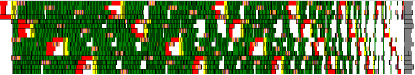
Figure 1: Profile of CALU using static scheduling on 16 cores of an AMD Opteron machine.

The emerging complexities of multi- and many-core architectures and the need for performance consistency suggests making codes more self-adaptive to the wide variety of different architectural characteristics that are difficult to predict. Examples of such self-adaptive techniques are work-stealing [6, 5] and openMP guided self-scheduling [20].

These self-adaptive strategies allow work to be dynamically scheduled to cores (during execution of the linear algebra routine), rather than to be statically scheduled (before execution of the routine). Using such dynamic scheduling techniques in numerical library routines gives the advantage that available threads execute tasks as soon as they are ready. Even if one thread becomes slow or inactive due to transient performance variation induced by system events such as I/O or OS daemons, the other threads will not be affected. The fundamental disadvantages of dynamic scheduling are the dequeue overhead and loss of data locality that these strategies introduce; the conventional static scheduling would not have caused overheads for such load balancing. The dequeue overhead to pull a task from a work queue can become non-negligible especially on an architecture with a large number of cores. Dynamic scheduling provides no guarantee for threads to reuse data resident in their local cache. The act of such dynamic migration of data has a significant cost, especially on architectures with large differences in access time between cache and main memory. Thus, due to these potentially large scheduling overheads, it may seem more appropriate to simply continue to use conventional static scheduling for these cases.

What is needed for such codes is a tunable scheduling strategy that maintains load balance across cores while also maintaining data locality and low dequeue overhead. To achieve this, we use a strategy that combines static and dynamic scheduling. This approach was shown to be successful on regular mesh computations [16]. This tunable scheduling strategy allows us to flexibly control the percentage of tasks that can be scheduled dynamically; this gives to a knob to control load balancing so that it occurs only at the point in computation when the benefits it provides outweighs the costs it induces. On NUMA machines where remote memory access is costly, the percentage of work scheduled dynamically should be small enough to avoid excessive cache misses, but large enough to keep the cores busy during idle times in the static part.

In this work, we show the effectiveness of this method in the context of already highly-optimized dense matrix factorizations. We focus in particular on communication avoiding LU (CALU), a recently introduced algorithm which offers minimal communication [12]. We choose LU because of its tight synchronization and communication constraints. Most of the discussion applies to other routines in dense numerical linear algebra also. Our prior work on multi-threaded CALU [8] was based on dynamic scheduling. The algorithm performed well on tall and skinny matrices, but became less scalable on square matrices with increasing numbers of processors. When the input matrix is tall and skinny, the fast factorization of the panel usually surpasses the various types of scheduler optimizations. However, when the matrix is large, it becomes important to modify the properties of the scheduler to take into account memory bandwidth bottlenecks and data locality.

In our hybrid scheduling approach, the percentage of computation that allotted to be dynamic scheduled can be tuned based on the underlying architecture and the input matrix size. An important factor that impacts performance is the data layout of the input matrix. Hence, we also investigate three data layouts: a classic column major format, a block cyclic layout, and a two level block layout. Table 1 describes the design space we explore. By avoiding load balancing until it is absolutely needed, we are able to acheive significantly higher performance gains over a fully static or a fully dynamic scheduling strategy, and also can provide better performance compared to two well-known numerical linear algebra libraries, MKL and PLASMA. While the paper focuses specifically on CALU, most of the discussion applies to other methods of factorization such as QR, rank-revealing QR, and to a certain degree the Cholesky and $LDL^{T}$ factorizations.

	CALU
Data Layout $\backslash$ Scheduling	Static	Dynamic	static (number%
			dynamic)
Block cyclic layout (BCL)	$\surd$	$\surd$	$\surd$
2-level block layout (2l-BL)	$\surd$	$\surd$	$\surd$
Column major layout (CM)		$\surd$

Table 1: Design space. In the hybrid version, number% represents the percentage of the dynamic part

This paper is organized as follows. In the section 2, we briefly give a background of LU and CALU factorization. In the section 3, we show how to combine static and dynamic scheduling to achieve good performance in numerical librairies. In section 4, we discuss the data layout we use for the matrices. In section 5, we present experimental results. In section 6, we present a theoretical analysis. In section 7, we present a discussion and broader impact to future machines(e.g. exascale). In section 8, we discuss relevant related work. In section 9, we conclude the paper and discuss future work.

2 Direct methods in dense linear algebra

In this section we briefly introduce the direct methods of factorization, and in particular the LU factorization and its communication avoiding variant, CALU. The LU factorization decomposes the input matrix $A$ of size $m\times n$ into the product of $L\cdot U$, where $L$ is a lower triangular matrix and $U$ is an upper triangular matrix. In a block algorithm, the factorization is computed by iterating over blocks of columns (panels). At each iteration, the LU factorization of the current panel is computed, the $U$ factor of the current block row is determined, and then the trailing matrix is updated. This last step is computationally the most expensive part of the algorithm. It can be performed efficiently since it exploits BLAS 3 operations, and it exposes parallelism. The panel factorization, even if it does not dominate the computation in terms of flops, is a bottleneck in terms of parallelism and communication. This is because the update of the trailing matrix can be performed only once the panel is factored. Hence, it is important to perform the panel factorization as fast as possible. For example, the multithreaded LAPACK [3] performs the panel factorization sequentially, and this leads to poor performance, even if the update is performed in parallel.

However, due to partial pivoting, its parallelization is not an easy task. The panel factorization requires communication (or synchronization in a shared memory environment) for the computation of each column, and this leads to an algorithm which communicates asymptotically more than what the lower bounds on communication require. An efficient sequential algorithm is the recursive LU factorization [23, 13]. However, a parallelization of this approach will likely have scalabiltity limits due to the recursive formulation of the algorithm.

Communication avoiding algorithms introduced in the last years provide a solution to this problem. In the case of the LU factorization, its communication avoiding version CALU [12] uses a different pivoting strategy, tournament pivoting, which is shown to be as stable as partial pivoting in practice. With this strategy, the panel factorization can be efficiently parallelized, and the overall algorithm is shown to provably minimize communication. The panel factorization, refered to as TSLU, is computed in two steps. The first preprocessing step identifies, with low communication cost, pivots that can be used for the factorization of the entire panel. These pivots are permuted into the diagonal positions, and the second step computes the LU factorization with no pivoting of the entire panel. The preprocessing step is performed as a reduction operation, with LU factorization with partial pivoting being the operator used at each step of the reduction. We use a binary tree for the reduction, which is known to minimize communication.

In CALU, the panel factorization remains on the critical path. However, current research indicates that this is required for obtaining a stable pivoting strategy and a stable factorization. A different pivoting strategy known as block pairwise pivoting removes the panel factorization from the critical path, but this strategy requires more investigation in terms of stability. This approach was explored in previous versions of PLASMA [7] and FLAME [21].

The scheduling strategy that we present in the following section relies on the task dependency graph of CALU. We consider that the input matrix $A$ is partitioned into blocks of size $b\times b$ as

$$A=\begin{pmatrix}A_{11}&A_{21}&\ldots&A_{1N}\\ A_{21}&A_{22}&\ldots&A_{2N}\\ \vdots&\vdots&&\vdots\\ A_{M1}&A_{M2}&\ldots&A_{MN}\end{pmatrix},$$

where $M=m/b$ and $N=n/b$.

The task dependency graph is obtained by considering that the computation of each block $A_{ij}$ is associated with a task. We distinguish the following tasks:

• task P: participates in the preprocessing step of the panel factorization TSLU.

• task L: computes part of the $L$ factor of the current panel, by using the pivots identified in task P.

• task U: computes a block of the $U$ factor in the current row.

• task S: updates a block of the trailing matrix.

With these notations, a matrix partitioned into $4\times 4$ blocks is showed in Figure 2, and its task dependency graph (DAG) is displayed in Figure 3.

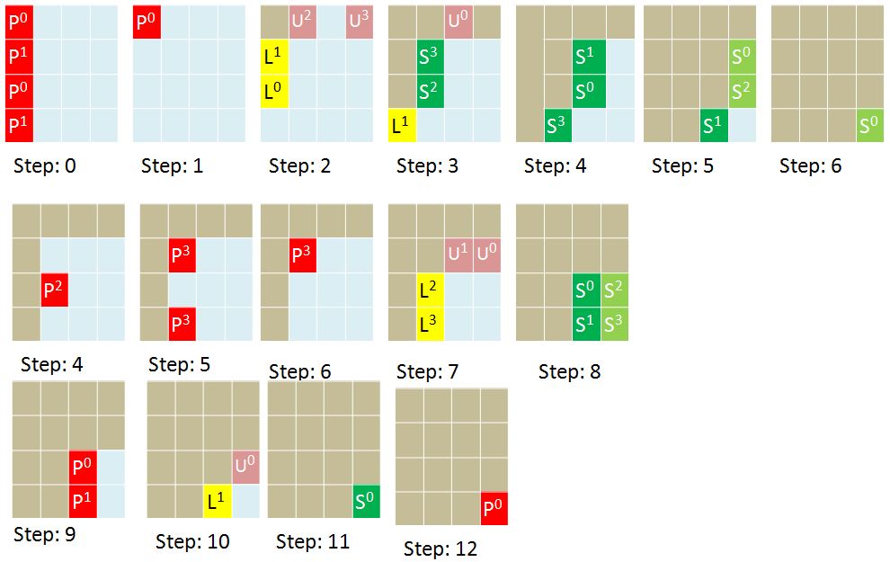
Figure 2: Example of execution of CALU static(20%) dynamic on a matrix partitioned into $4\times 4$ blocks using P=$4$ threads.

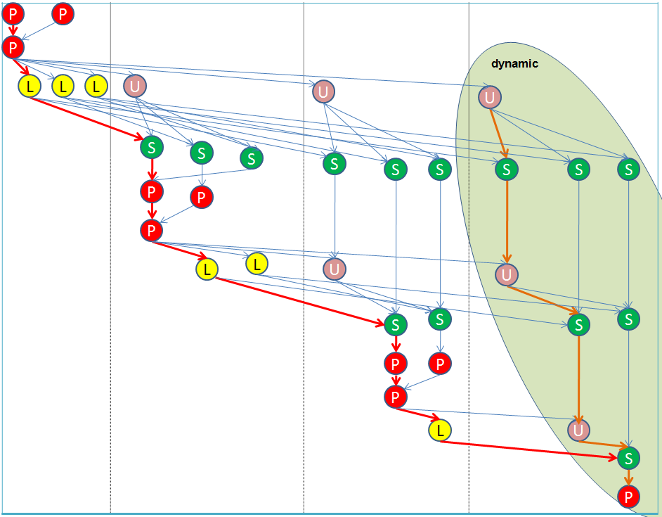
Figure 3: Task dependency graph of CALU static/dynamic of a matrix partitioned into $4\times 4$ blocks. The red arrows indicate the critical path of the static section of the algorithm, while the green arrows indicate the critical path of the dynamic section of the algorithm.

3 Scheduling based on a hybrid static/dynamic strategy

In this section, we describe our hybrid static/dynamic scheduling strategy that aims at exploiting data locality, ensuring good load balance, reducing scheduling overhead, and being able to adapt to dynamic changes in the system. The hybrid scheduling is obtained by spliting the task dependency graph into two parts, a first part which is scheduled statically, and a second part which is scheduled dynamically. Given a parameter $N_{static}$, tasks that operate on blocks belonging to the first $N_{static}$ panels are scheduled statically, while tasks that operate on blocks belonging to the last $(N-N_{static})$ panels are scheduled dynamically. Hence, the tasks that lie on the critical path of the algorithm are scheduled statically. During the factorization, each thread executes in priority tasks from the static part, to ensure progress in the critical path of the algorithm. When there are no ready static tasks, then the thread picks up a task from the dynamic part. Thus, the two parts of the task dependency graph are not independent.

Algorithm 1 describes CALU with hybrid static/dynamic scheduling. In the static part of the DAG, the matrix is distributed to threads using a classic two-dimensional block-cyclic distribution. The algorithm proceeds as follows. For the first $N_{static}$ iterations, once the panel $K$ is factored statically, several tasks become ready. These tasks are grouped into two distinct sets. The first set is formed by tasks that update blocks $A_{:,J}$, with $K+1\leq J\leq N_{static}$. These tasks are scheduled statically. They are inserted into the queue of ready tasks of the thread which owns the blocks $A_{:,J}$. The second set is formed by tasks that operate on blocks $A_{:,J}$ with $N_{static}<J\leq N$. These tasks are scheduled dynamically, they are inserted in a shared global queue of ready tasks. For clarity of the presentation, the algorithm does not present the insertion of ready tasks in the dynamic queue.

For the last $N-N_{static}$ iterations, the algorithm uses a fully dynamic scheduler. While the same pattern of execution is used as in the static part, the main difference is that now the tasks are scheduled dynamically when they are ready.

The static part of Algorithm 1 uses the routine "dynamic_tasks()", which is described in Algorithm 2. This routine selects one task in the dynamic part of the matrix when a thread requests it. The task is selected by traversing the DAG associated with the dynamic part using a depth- first search approach. With this approach, the columns are updated from left to right. This ensures that the execution follows in priority the critical path when the algorithm will reach the dynamic section. The tasks selected by the routine are removed from the global queue.

We note that a static/dynamic approach makes two critical paths appear. The first path corresponds to the critical part of the task dependency subgraph scheduled statically. In our case, this corresponds to the critical path of the whole task dependency graph of CALU. The second path corresponds to the critical path of the task dependency subgraph scheduled dynamically. The two paths are displayed in Figure 3 on our task dependency graph example. The second path is executed in parallel with the first one. We consider the second path as important as the first one; otherwise, the algorithm can stagnate when it arrives at the dynamic section.

We use the following notation and routines in Algorithm 1:

• I_Own(panel(K)): returns true if the thread executing this instruction owns a block of panel $K$.

• I_Own(block-row(K)): returns true if the thread executing the instruction owns a block of block-row $K$.

• task P: each thread executing this task performs a reduction operation to identify $b$ pivots that will be used for the panel factorization of the current panel. The reduction operator is Gaussian elimination with partial pivoting, and for this the best available sequential algorithm can be used. In our experiments we use recursive LU [23].

• "do task L (on $L_{K:M,K}$) in parallel": computes the $L$ factor of panel $K$ in parallel. In the static section, each thread computes the blocks of $L$ of panel $K$ that it owns. In the dynamic section, available threads compute blocks of $L$ of panel $K$ until the whole panel is finished.

• "do task S (on $A_{K+1:M,J}$) in parallel": panel $J$ is updated in parallel. In the static section, each thread updates the blocks of panel $J$ that it owns (if any). In the dynamic section, available threads update blocks of panel $J$ until the whole panel is finished.

Algorithm 1 CALU with hybrid static/dynamic scheduling

1:  Input: $m\times n$ matrix $A$, block size $b$, percentage of dynamic section $d_{ratio}$

2:  $N_{static}=N*(1-d_{ratio})$

3:  /* static section*/

4:  for $K$ = $1$ to $N_{static}$ do

5:      if I_Own(panel(K)) then

6:       do task P Preprocessing of TSLU($A_{K:M,K}$) in parallel

7:      endif

8:      while $taskP[K]$ not done

9:       do dynamic_tasks()

10:      end while

11:      Let $\Pi_{KK}$ be the permutation performed for panel $K$ such that $\Pi_{KK}A_{1:b,1:b}=L_{KK}U_{KK}$

12:      do task L $L_{K:M,K}=A_{K:M,K}U_{KK}^{-1}$ in parallel

13:      if I_Own(block-row(K)) then

14:       for $J$ = $K+1$ to $N_{static}$

15:        if I_Own(panel(J)) then

16:         do right swap $A_{K:M,J}=\Pi_{KK}A_{K:M,J}$

17:         do task U $U_{K,J}=L_{KK}^{-1}A_{K,J}$

18:        endif

19:       end for

20:      endif

21:      for $J$ = $K+1$ to $N_{static}$

22:       if I_Own(panel(J)) then

23:        while the block $U_{K,J}$ not computed

24:         do dynamic_tasks()

25:        end while

26:        do task S $A_{K+1:M,J}-=L_{K+1:M,K}U_{K,J}$ in parallel

27:       endif

28:      end for

29:  end for

30:  /* dynamic section*/

31:  for $K$ = $N_{static}$ to $N$ do

32:      do task P Preprocessing of TSLU($A_{K:M,K}$) in parallel and dynamically

33:      Let $\Pi_{KK}$ be the permutation performed for panel $K$ such that $\Pi_{KK}A_{1:b,1:b}=L_{KK}U_{KK}$

34:      do task L $L_{K:M,K}=A_{K:M,K}U_{KK}^{-1}$ in parallel and dynamically

35:      for $J$ = $K+1$ to $N$ do in parallel and dynamically

36:       do task U $A_{K,J}=L_{KK}^{-1}A_{K,J}$

37:      end for

38:      for $J$ = $K+1$ to $N$ do in parallel and dynamically

39:       do task S $A_{K+1:M,J}$ -= $L_{K+1:M,K}U_{K,J}$ in parallel

40:      end for

41:  end for

42:  /* Apply permutations to the left */

43:  $L_{1:M,1:N}=\Pi_{NN}\ldots\Pi_{11}L_{1:M,1:N}$ in parallel   /* dlaswap */

Algorithm 2 dynamic_task

1:  Let $K_{0}$ be the panel currently computed in the static section.

2:  for $J$ = $N\_STATIC+1$ to $N$ do

3:      for $K$ = $1$ to $K_{0}-1$ do

4:       if $U_{K,J}$ not computed

5:        do task U $U_{K,J}=L_{KK}^{-1}A_{K,J}$

6:       endif

7:       if $A_{:,J}$ not updated by panel $K$

8:        do task S $A_{I,J}=A_{I,J}-L_{I,K}*U_{K,J}$ for all $I$ with $K+1\leq I\leq M$

9:       endif

10:      endfor

11:  end for

We show an example of execution of our algorithm on the same matrix formed by $4\times 4$ blocks from Figure 2 and its task dependancy graph from Figure 3. In Figure 2, the exponent indicates the thread which executes the task. At steps 5 and 6, we observe that instead of becoming idle while waiting for the completion of the factorization of the third panel, two threads execute a task from the dynamic section. This avoids unnecessary idle time.

In our current work, the percentage of the dynamic part $d_{ratio}$ is a tuning parameter, which determines the number of panels that will be executed statically ($N_{static}$) or dynamically ($N-N_{static}$). It is therefore possible to switch from a 100% static version to a 100% dynamic version. In practice, a particular scheduling technique can be highly efficient on one architecture, but less efficient on another. In the experiemental section, we show that the best scheduling strategy depends not only on the architecture on which it is executed, but also on the size of the matrix, the data layout of the matrix, and the number of processors. The flexibility to choose the percentage of the dynamic section in our algorithm will allow it to adapt on different architectures.

As explained in section 2, for factorizations that use some form of pivoting as CALU or Gaussian elimination with partial pivoting, the panel factorization lies on the critical path. In a fully static approach, this can be a bottleneck and may cause inactivity due to lack of tasks. The combined static/dynamic scheduling helps to overcome this problem. Threads that are idle waiting for the completion of the panel factorization perform tasks from the dynamic part. This is illustrated in Figure 4 where a static (20% dynamic) scheduling is used to factor a matrix of size $5000\times 5000$. The red tasks represent the panel factorizations and the green tasks represent the updating computation. We observe that some of the threads finish earlier than others the panel factorization. In a fully static approach, they would become idle. In the hybrid approach, they execute tasks from the dynamic section, and there is almost no idle time in this example.

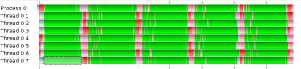
Figure 4: First steps of the factorization of a matrix of size $5000\times 5000$ using a static (20% dynamic) scheduling

Several other optimizations are used in our algorithm that are important for its performance, but we do not describe them in detail in this paper. For example, the static section employs look-ahead, a technique used in dense factorizations to allow the panel factorizations to be performed as quickly as possible. The granularity of the tasks used during the update of the trailing matrix has a direct impact on the performance of BLAS 3 operations (dgemm or cgemm in our case). The best granularity is a trade-off between parallelism (there should be enough tasks to schedule) and BLAS 3 performance. In the static section, a thread can update the blocks it owns one by one, or it can group them together and update using one single call to BLAS 3. The latter option leads to a better performance of BLAS 3, and also to a reduction in the number of messages transfered (if an appropriate data layout is used). However the number of words transfered stays the same. In our experiments, the threads update the trailing matrix by using blocks of size $kb,k\geq 1$, with $k=3$.

4 Data Layout

Classic libraries such as Lapack and Scalapack store the matrices using a column major layout. However, novel algorithms that minimize communication such as CALU require the usage of novel data layouts, based on blocking or recursive blocking. In this paper, we investigate the impact on performance of two data layouts that are adapted to our algorithm. We describe them in the following.

4.1 Block cyclic layout (BCL)

This layout aims at enabling data locality in the static section of our algorithm. The static section considers that the matrix is distributed using a 2D block cyclic layout over a 2D grid of threads. Then, during the algorithm, each thread modifies the blocks that it owns. The block cyclic layout stores contigously in memory, for each thread, the blocks that it owns. In other words, the matrix is partitioned into as many submatrices as threads. Each submatrix is stored in memory using a column major layout. Note that a submatrix is formed by blocks issued from the 2D block cyclic layout; that is, their column indices and row indices are not contiguous (except inside the small blocks of size $b\times b$).

The block cyclic layout is displayed at the left of figure 5. The matrix was partitioned into blocks of size $2\times 2$ which were distributed using the 2D block cyclic layout over a grid of 4 threads. The main avantage of this storage compared to full column major layout as implemented in LAPACK is that in the static section, the data of each thread is stored contiguously in its local memory. Another avantage is the possibility of improving BLAS 3 performance, described in the previous section. Each thread can simply call dgemm (or cgemm) on a block which can be larger than $b\times b$.

4.2 Two level block layout (2l-BL)

This layout can be seen as a recursive block layout, with the recursion being stopped at depth two (with the exception that at the first level, the matrix is partitioned using a block cyclic layout). At the second level of the recursion, the submatrix belonging to each thread is further partitioned into blocks of size $b\times b$ and each block is stored contigously in memory. This partitioning is shown at the right of Figure 5. The main avantages of this storage is that, with an appropriate value of $b$, the block (sometimes refered as tile) can fit in cache at some level of the hierarchy. Hence any operation on the block can be performed with no extra memory transfer.

However, with this layout, it is not straightforward to increase the size of the blocks used during the update of the trailing matrix using BLAS 3. This would require a copy of the data, which could add extra time. We do not explore this option in this paper.

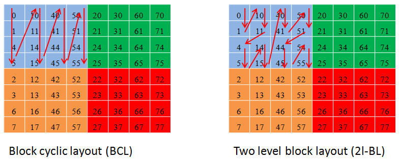
Figure 5: Data layout. The figure at left displays the partitioning of the matrix into four blocks using a 2D block cyclic layout (BCL) based on blocks of size $b\times b$. Each of the four blocks is stored contiguously in memory. The figure at right displays the two level block layout (2l-BL) layout, which further stores contigously in memory blocks of size $b\times b$ for each of the four blocks.

5 Experimental results

In this section we evaluate the performance of our algorithms on a four-socket, quad-core machine based on Intel Xeon EMT64 processor and on an eight-socket, six-core machine based on AMD Opteron processor running on Linux. The Intel machine has a theoretical peak performance of 85.3 Gflops/second in double precision. Each core has a frequency of 2.67GHz, a private L1 cache of size 32 Kbytes, an L2 cache of size 512 Kbytes, and an L3 cache of size 8192 Kbytes shared with the others cores. The AMD machine has a theoretical peak performance of 539.5 Gflops/second in double precision. Each core has a frequency of 2.1 GHz, a private L1 cache of size 64 Kbytes, a private L2 cache of size 512 Kbytes, and an L3 cache of size 5118 Kbytes shared with the other cores of the same socket.

We first present the performance of the hybrid static/dynamic scheduling compared to a fully static and a fully dynamic scheduling, while also discussing the impact of the data layout on performance. We then compare the performance with the corresponding routines from MKL 10.3.2 vendor library and PLASMA 2.3.1.

5.1 Performance of static/dynamic scheduling

In the following, CALU static refers to the version of CALU based on fully static scheduling, while CALU dynamic refers to the version of CALU based on fully dynamic scheduling. CALU static/dynamic refers to the version of CALU based on combined static and dynamic scheduling. When we want to identify the percentage of the dynamic part, we use CALU static(number% dynamic), where number% specifies the percentage of the computation scheduled dynamically.

5.1.1 Comparison with static and dynamic scheduling using block cyclic layout

We first discuss the performance of CALU using a block cyclic layout. As explained earlier, one of the advantages of this layout is that during the update of the trailing matrix, we can call dgemm on larger blocks by grouping together blocks that are stored in the same memory. While we can group together blocks that share the same rows or the same columns, we choose the latter option such that the algorithm can make progress on its critical path.

Figure 6 shows the performance of CALU static, CALU dynamic and CALU static/dynamic with varying the percentage of the dynamic scheduled work on the 16 core Intel Xeon machine. We observe that hybrid static/dynamic scheduling is more efficient than either of static or dynamic scheduling. In particular, CALU static(10% dynamic) is 8.20% faster than CALU static, and is 1.4% faster than CALU dynamic. However,the difference obtained by varying the percentage of the dynamic section is not significant. On this machine, the static scheduling is the least efficient, while the dynamic scheduling is closer to the best performance obtained by the static/dynamic approach. This performance is explained by the fact that the scheduler overhead and the cache miss penalties of the dynamic approach are less significant than the idle time introduced by load imbalance in the static approach.

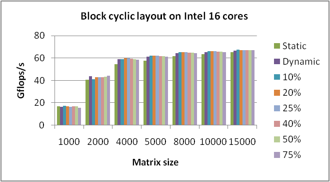
Figure 6: Performance of CALU with static/dynamic scheduling on Intel 16-core machine. The percentage of the dynamic part is varied from 10% to 75%. The matrix of size $M=N=5000$ is stored using block cyclic layout.

Figure 7 shows the performance obtained on the 48 core AMD Opteron machine. On NUMA machines, the memory latency plays an important role on performance. Static scheduling is very appropriate in this case because of its good use of data locality. However, the best performance is obtained by combining static with a small percentage of dynamic (10% or 20%), which is sufficient to reduce the thread idle time that cannot be handled by using purely static scheduling.

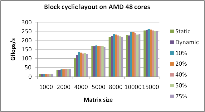
Figure 7: Performance of CALU with static/dynamic scheduling on the 48 core AMD opteron machine. The percentage of the dynamic part is varied from 10% to 75%. The matrix is stored using the block cyclic layout.

Figure 8 shows the percentage of improvement of CALU static(10% dynamic) and CALU static(20% dynamic) over CALU static and CALU dynamic. The best improvement is observed on 48 cores with $M=N=4000$, where CALU static(10% dynamic) is 30.3% faster than CALU static and 10.2% faster than CALU dynamic. For $M=N=10000$ on 48 cores, CALU static(10% dynamic) is 6.9% faster than CALU static and 8.4% faster than CALU dynamic. This suggests that, especially for smaller matrices, using just a small percentage of dynamic scheduling can provide significant performance benefits. When we do these experiments using only 24 cores, CALU static(20% dynamic) is slightly faster than CALU static(10% dynamic). This suggests that in some cases, increasing the percentage of dynamic scheduling could lead to better performance, and that this percentage should be appropriately tuned.

a. Experiments on 24 cores

b. Experiments on 48 cores

Figure 8: Percentage of improvement of CALU static(10% dynamic) and CALU static(20% dynamic) over CALU static and CALU dynamic on the AMD 48-core machine. The matrix is stored using a block cyclic layout.

5.1.2 Comparison with static and dynamic scheduling using 2-level block layout

We now discuss the performance of CALU when using a 2-level block layout. Figure 9 shows the performance obtained on 16 cores Intel Xeon machine. The behavior is the same as observed with the block cyclic layout. Increasing the percentage of dynamic in CALU static/dynamic does not have an important impact on performance. Again, the static scheduling is less efficient than all the other approaches. The best improvement is obtained with CALU static(10% dynamic) for $M=N=4000$, when it is 10.6% faster than static and 1.7% faster than dynamic.

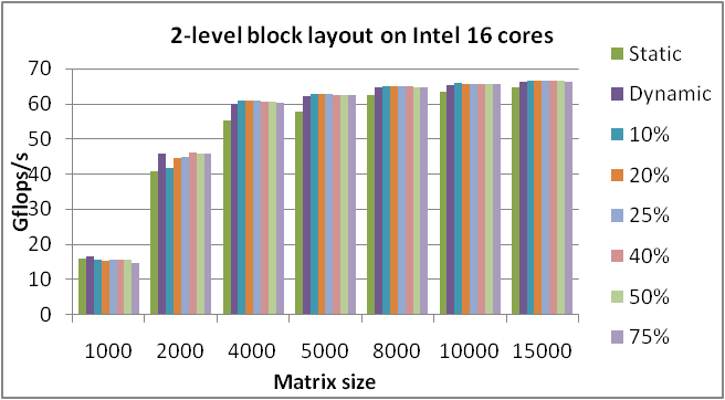
Figure 9: Performance of CALU with static/dynamic scheduling on Intel 16 core machine. The percentage of the dynamic part is varied from 10% to 75%. The matrix is stored using 2-level block layout.

Figure 10 shows the performance obtained on the 48 core AMD Opteron machine. In this case, varying the percentage of the dynamic part in the hybrid static/dynamic scheduling leads to important differences in performance. CALU dynamic is the least efficient approach. There are three main reasons for this. First, the blocks are stored contiguously in memory such that they fit in cache, but due to the dynamic scheduling, the data might not be reused. Second, when the matrix size increases along with the number of blocks, the dequeue overhead of the dynamic scheduler becomes significant. Third, due to the storage of the matrix, we do not group blocks together to improve the performance of BLAS operations and reduce scheduling overhead. Due to these reasons, increasing the percentage of the dynamic part in CALU static/dynamic does not lead to better performance.

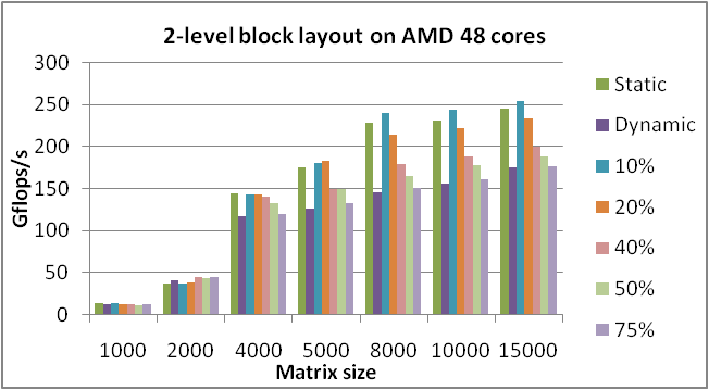
Figure 10: Performance of CALU with static/dynamic scheduling on AMD Opteron 48 core machine. The percentage of the dynamic part is varied from 10% to 75%. The matrix is stored using 2-level block layout

Figure 11 shows the percentage of improvement of CALU static(10% dynamic) and CALU static(20% dynamic) over CALU static and CALU dynamic. In the best case, CALU static(10% dynamic) is 5.9% faster than static, and 64.9% faster than dynamic on 48 cores. On 24 cores, CALU static(10% dynamic) is up to 10% faster than CALU static, and up to 16% faster than CALU dynamic.

a. Experiments on 24 cores

b. Experiments on 48 cores

Figure 11: Percentage of improvement of CALU static(10% dynamic) and CALU static(20% dynamic) over CALU static and CALU dynamic on AMD 48 core machine. The matrix is stored using a 2-level block layout.

5.1.3 Summary of results

Figures 12 and 13 show a summary of our results on both machines. (In the figures, dynamic rectangular refers to a column major layout of the input matrix.) We note that the performance of the algorithm depends on the matrix size, the data layout used, and is architecture dependent. However several trends appear. On the Intel Xeon machine, the dynamic scheduling is fairly efficient. For this machine, the time to transfer data from main memory to the cache of each core does not hinder the performace of a fully dynamic scheduling strategy. However, on a NUMA machine like the AMD Opteron, fully dynamic scheduling is highly inefficient due to the cost of cache misses, and so exploiting locality through constraining data migration is essential on such a machines.

When the matrix is small ($n\leq 5000$), the two-level block cyclic layout leads to good performance. But with increasing matrix size, the block cyclic layout leads to better performance than the two-level block layout. This is mainly due to our approach of performing BLAS 3 operations on larger blocks when the block cyclic layout is used. When the matrix is large enough, there are enough tasks to schedule, the synchronization is reduced, and the BLAS 3 operations are more efficient.

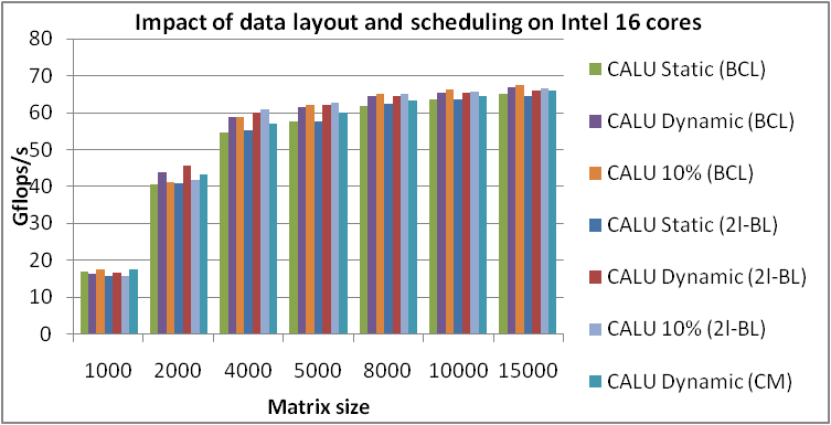
Figure 12: Impact of data layout and scheduling on the Intel 16 core machine.

In general, CALU static with a small percentage of dynamic leads to the best performance gains, and can achieve performance that is closer to peak performance on both machines. On the Intel machine, CALU static(10% dynamic) achieves up to $67.4$ Gflops/s, which is $79$% of the peak performance. On the AMD machine, CALU static(10% dynamic) achieves up to $264.1$ Gflops/s that is $49$% of the peak performance. Both results were obtained for a matrix of size $m=n=15000$ stored using a block cyclic layout.

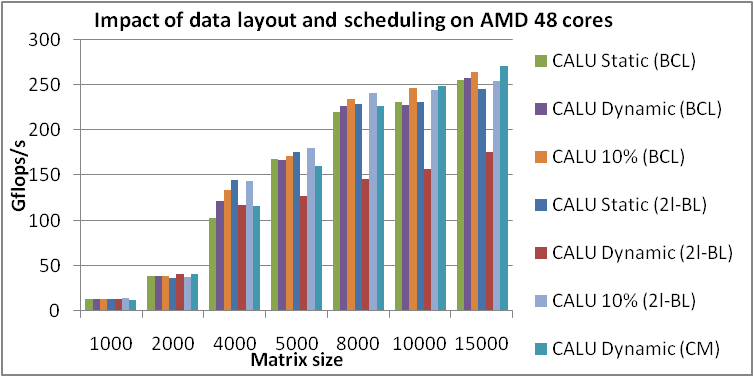
Figure 13: Impact of data layout and scheduling on AMD 48 core machine.

5.2 Profiling

We observe the timelines of our algorithm on a matrix of size $2500\times 2500$ with a block size of $b=100$ using 16 cores of the AMD machine. Figure 14 shows the profiling of the dynamic version of CALU using a column major layout. We observe that 90% of threads become idle after only 60% of the total factorization time, while for the other variants of scheduling, this happens towards the very end, after 80%-90% of the total factorization time.

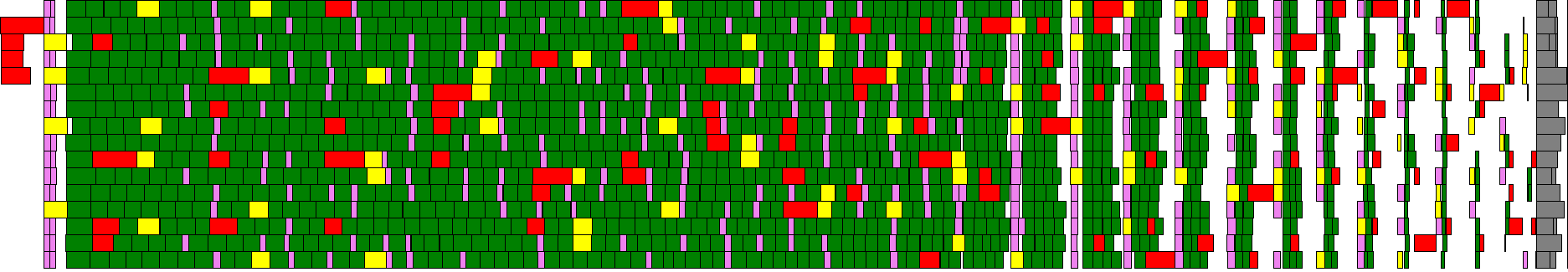
Figure 14: CALU dynamic with column major layout on AMD machine.

As presented in the Introduction, Figure 1 shows the profiling of the static version of CALU, we observe pockets of idle times during the factorization.

Figure 15 shows the profiling of static(10% dynamic) version of CALU. We observe that a small percentage of dynamic helps to keep the cores busy, and reduces drastically the idle time.

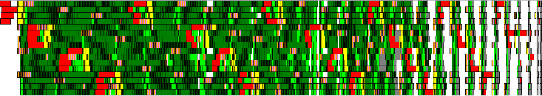
Figure 15: CALU static (10% dynamic) with 2-level block layout on AMD using 16 cores

5.3 Comparison with MKL and PLASMA

We compare in Figures 16 and 17 the performance of CALU static(10% dynamic) against the dgetrf routine from MKL and dgetrf_incpiv from PLASMA. The routine from MKL implements Gaussian Elimination with partial pivoting. Since the initial data placement may have a dramatic impact on the performance of an application running on NUMA machines [17], we distribute the input matrix to all the cores before calling MKL. This distribution was done using existing numactl (with argument –interleave), which controls NUMA policy for shared memory. This improves dramatically the performance of the routine MKL_dgetrf on the AMD 48 core machine.

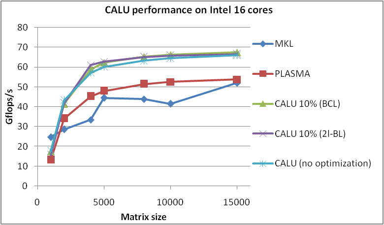
Figure 16: Performance of CALU, MKL, and PLASMA on the 16 core Intel machine.

Our algorithm outperforms MKL on both the Intel and AMD machines. On the 16 core Intel Xeon machine, for $M=N=10000$, CALU static(10% dynamic) with both BCL layout and 2l-BL layout is about $60\%$ faster than MKL. The best improvement is obtained with CALU static(10% dynamic) (2l-BL) for $M=N=4000$, where it is $82\%$ faster than MKL. On the 48 core AMD machine, for $M=N=10000$, CALU static(10% dynamic) with both data layouts is about $100\%$ (up to $110\%$ faster than MKL.

We also observe improvements (up to $20\%$ - $30\%$ for larger matrices) with respect to the dgetrf_incpiv routine from PLASMA. This routine implements the LU factorization using incremental pivoting (which can be seen as a block version of pairwise pivoting, whose stability is still under investigation), in which the panel factorization is removed from the critical path. This leads to a task dependency graph that is different from CALU’s task dependency graph. In the recently released version of PLASMA, there is also an implementation of Gaussian elimination with partial pivoting, but we do not have a thorough comparison against this new routine for the moment.

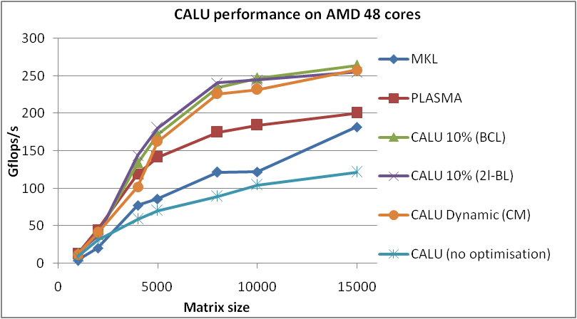
Figure 17: Performance of CALU, MKL, and PLASMA on the 48 core AMD Opteron machine.

6 Theoretical Analysis

To understand these results, we provide a basic performance model and theoretical analysis. Because we want to avoid load balancing as much as possible until it is absolutely needed(due to the overheads it incurs, such as coherence cache misses and dequeue overhead), we aim to minimize the percent dynamic. Thus, we ask the following question: given a particular algorithm and a particular architecture, what is the minimum percentage dynamic $d_{ratio}$(defined in the algorithm section) that should be used in an algorithm to obtain the best performance? To understand this, we formalize the problem as follows. Let $f_{s}$ the fraction of work done statically. Note the $d_{ratio}=1-f_{s}$. Let $p$ be the number of cores. Let $T_{1}$ be the serial time for the computation. Let $T_{p}$ = $\frac{T_{1}}{p}$ be the time for computation to be done in parallel across $p$ cores. We formalize our question by asking the following: what is the largest static fraction $f_{s}$ that will make it feasible to attain ideal execution time $t_{ideal}$, given a compute core $i$ has excess work ${\delta}_{i}$? Let ${\delta}_{max}$ be the maximum excess work across all cores. Let ${\delta}_{avg}$ be the average excess work across all cores. Theorem 1 provides the bound for this static fraction.

Theorem 1: $f_{s}\leq 1-\frac{{\delta}_{max}-{\delta}_{avg}}{T_{p}}$
Proof: In the presence of some excess work ${\delta}_{i}$ (e.g. system noise) that is forced on core $i$, let $t_{ideal}$ be the ideal time for computation for a given number of cores $p$ when excess work can be load balanced, and let $t_{actual}$ be the worst-case time taken when the excess work cannot be load balanced. This means that:

$t_{ideal}=\frac{T_{1}+\sum_{i=1}^{n}{\delta_{i}}}{p}$ and $t_{actual}=f_{s}\times\frac{T_{1}}{p}$ $+$ $\max{{\delta}_{i}}$

To find the breakpoint at which static scheduling will induce load imbalance, we set $t_{actual}\leq t_{ideal}$. Given this, the time for the case when the compuation is load imbalanced, $t_{actual}$, will be is no worse than the case of completely load balanced computation, $t_{ideal}$. Expanding this inequality, we have:

$f_{s}\times\frac{T_{1}}{p}+\max_{i=1}^{p}{{\delta}_{i}}$ $\leq$ $\frac{T_{1}+\sum_{i=1}^{n}{\delta_{i}}}{p}$

Solving for the static fraction $f_{s}$, we have:

$f_{s}\leq\left(\frac{T_{1}+\sum_{i=1}^{n}{\delta_{i}}}{p}-\max_{i=1}^{p}{\delta_{i}}\right)\times\frac{p}{T_{1}}$

$=$ $f_{s}\leq\frac{T_{1}+\sum_{i=1}^{n}{\delta_{i}}}{T_{1}}-\frac{\max_{i=1}^{p}{\delta}_{i}\times p}{T_{1}}$

$=$ $f_{s}\leq 1-\frac{{\left(\max_{i=1}^{p}{\delta}_{i}\right)\times p}-\sum_{i=1}^{n}{\delta_{i}}}{T_{1}}$

$=$ $f_{s}\leq 1-\frac{{\left(\max_{i=1}^{p}{\delta}_{i}\right)}-\frac{\sum_{i=1}^{n}{\delta_{i}}}{p}}{\frac{T_{1}}{p}}$

Based on our assumptions of $T_{p}$, and our definition of $\delta_{max}$, $\delta_{avg}$:

$f_{s}\leq 1-\frac{\delta_{max}-\delta_{avg}}{T_{p}}$

Note that this analysis assumes that parallel time includes no overheads. Due to the communication on critical path of LU(even for the communication-avoiding case), a full analysis of our LU factorization cannot ignore the term of communication cost, $T_{criticalPath}$. If $p\prec$ $\frac{T_{1}}{T_{criticalPath}}$, the $T_{criticalPath}$ does not dominate the total execution time of parallel CALU. Our analysis presented is easily extensible though for the case when $p$ $\geq$ $\frac{T_{1}}{T_{criticalPath}}$; this term of communication cost can be added to the denominator. Thus, the denominator will be $\frac{T_{1}}{p}+T_{criticalPath}$. If we also assume there is a cost of migration of tasks $T_{migration}$(due to coherence cache misses that scheduling incurs), then the denominator becomes $\frac{T_{1}}{p}+T_{criticalPath}+T_{migration}$. The model can be made even more accurate by incorporating other costs of load balancing (e.g. dequeue overheads) as well. In general, these additional relevant costs can be captured by adding a single term, $T_{overhead}$ to the term in the denominator $\frac{T_{1}}{p}$, effectively providing a more realistic value for $T_{p}$ that incorporates both communication cost and load balancing cost.

This simple theoretical analysis allows us to more clearly understand the impact of application parameters to our experimental results. Given the time complexity of the parallelized version of the computation $T_{p}$ of a dense factorization (again assuming there is no cost of data movement),the above formula gives us the ability to plug in the expression for $T_{p}$ to find the upper-bound on the static fraction. Increasing matrix size can cause an increase in $T_{1}$ in Theorem 1. From Theorem 1, we see that increasing matrix size allows us to increase the maximum static fraction that we can use. In general, as the total cost of the algorithm $T_{1}$ increases and we keep two architectural parameters $p$ and $\delta_{max}-\delta_{avg}$ constant, we can use a larger percent static to avoid scheduling overheads.

The static fraction can also be affected by architectural parameters. On the Intel machine, for example, communication compared to computation is negligible, due to the low-latency of coherence cache miss. This decreases percentage of dynamic fraction, and increases the static fraction $f_{s}$. Thus, as the penalty for coherence cache misses becomes higher, the percentage static will need to increase to avoid such coherence cache misses.

7 Discussion

A more detailed performance model and theoretical analysis for regular mesh codes has been established through the follow-up studies of the work by V. Kale et al [16]. The adoption of this model will allow us to calculate expected completion time of a dense matrix factorization in the presence of transient load imbalance occurring with some probability. Given this, we can couple our performance model with auto-tuning techniques and heuristics[10] for optimizing the scheduling strategy for a particular architecture, allowing us to significantly prune the search space of parameter configurations for our scheduling approach.

The problem of noise amplification has been projected (most recently through simulation) to seriously impede performance at very large scale [14]. In earlier work [16], it was shown that by improving performance consistency of the 3D regular mesh code, one can mitigate the impact of the noise amplification problem. The early results of the reduced standard deviations of wall clock times across multiple runs of our code under our tuned scheduling strategy is in accord with the performance consistency results shown in  [16].

With our theoretical analysis, we can provide projections for the upper-bound on the static fraction to be used within many-core nodes of an exascale machine. Keeping the work per core constant, the term $\left(\delta_{max}-\delta_{avg}\right)$ can increase in the presence of noise amplification. Given this and using Theorem 1, we project that the lower-bounds for percentage dynamic for numerical linear algebra routines will have to increase for use on future high-performance clusters.

8 Related work

The idea of combining static and dynamic scheduling has been studied in different contexts in the literature, but to the best of our knowledge none of the approaches focuses on dense numerical linear algebra. V. Kale et al. suggested a hybrid static/dynamic approach in [16] that can be incorporated into current MPI implementations of regular mesh codes to improve the load balancing of the initial static decompositions. They show the performance of their strategy on a 3D jacobi relaxation problem. Our work here embraces the fundamental principles advocated in that paper, and applies it in the context of dense matrix factorizations. Xue et al. introduced an approach in [24] that improves the data locality when executing loop iterations in codes. This is done in the context of chip multi-processors. The authors show that the different loops of many codes may be decomposed into two parts: in one part, iterations are distributed across processors at compilation time; in the other part, iterations are distributed at runtime to available processors to improve the load balancing.

Our approach has some similarity with work-stealing, but proceeds more efficiently. In work stealing, the work is initially (statically) distributed almost equally to each thread. During the algorithm, each inactive thread (the thief) can pick a task from the queue of tasks of another thread (the victim). An important question is: from which other thread will this thread steal work? The approach of randomized work-stealing from the queue of another thread is implemented in Cilk [5]. Cilk is founded on theoretical analysis and proofs on its efficiency. It has been shown to offer acceptable performance, particularly for multi-programmed workloads on multi-cores.

In the LU factorization, the update of the trailing sub-matrix is performed from left to right, to maintain the execution of the algorithm on the critical path and to guarantee that the panel factorization will be able to start as soon as possible even if the updates of the columns of the previous steps are not completely done. In other words, columns close to the panel have high priority. Although random stealing can help balancing work among processors during execution, it might not follow the critical path of the factorization. In typical implementations of work stealing, when the queue of a particular thread is empty, that thread attempts to pick a task either at the top, or at the bottom, of a victim queue. Whether chosen from the top or the bottom of the queue, this approach is not optimal for many computations and in particular for dense factorizations. Picking a task at the beginning of the queue (FIFO) may lead to non-negligible synchronization overheads with the victim, or may cause false sharing due to two threads accessing data in two regions in memory in close proximity. While picking a task at the end of the queue (LIFO) may lead to acceptable load balancing in general, for computations in LU/CALU, the last columns have the least priority within the computation. This inhibits the progression of the critical path. Other work such as [22] suggest then the steal is done from the queue of the thread having the highest number of tasks. This cannot be applied directly to dense factorizations, where the number of tasks of a thread is not proportional to its workload.

9 Conclusions

We have designed and implemented a strategy that combines static and dynamic scheduling to improve data locality, load balancing, and exploit the power of current and emerging multi-core architectures. Our hybrid static/dynamic scheduling strategy applied to CALU leads to performance improvements over the fully static CALU and fully dynamic CALU, and also provides performance improvements over the corresponding routines in MKL and PLASMA. Our performance results show that the combination of static and dynamic scheduling is effective for dense communication avoiding LU factorization. In our experiements, we determine the best percentage of the dynamic part by running variations of the algorithm with different dynamic percentages. We show that, usually, 10% dynamic leads to good performance because it provides the best compromise between data locality, load balancing, and minimal dequeue overhead. While in this paper we focus on CALU, the same techniques can be applied to other dense factorizations as Cholesky, QR, rank revealing QR, $LDL^{T}$, and their communication avoiding versions. This remains future work.

On future high-performance clusters planned within the timespan of 5 years, often termed as exascale, each node will be comprised of many levels of parallelism, with possibly on the order of 100s of cores per node. Choosing between purely static and purely dynamic scheduling for numerical linear algebra routines will escape the problem of trying to gradual evolve, rather than radically change, our codes for use on emerging and future high-performance clusters. Our hybrid approach allows for self-adaptivity of the numerical linear algebra routines to the transient dynamic variations of the architecture, without loss of data locality that is so fundamentally important to a large class of HPC applications.

In future work, we opt to design a stronger model to determine the percentage of the dynamic section. We provide an approach to theoretically determine the percentage of the dynamic section, but we believe we can obtain even tighter bounds, given knowledge of scheduling costs. Furthermore, this theoretical analysis can be applied to other numerical linear algebra routines, as well as to full-fledged applications, given the expression for parallel execution time. We plan to enhance our scheduling technique so that tasks are chosen from the queue such that the data that these tasks operate on is highly likely to be in a core’s cache already, allowing for fewer coherence cache misses due to task migration. Such intelligent selection of tasks can be implemented by adding locality tags within the task data structure, and incorporating heuristics that make more accurate predictions on the task that is least likely to incur a migration overhead, if chosen.

References

- [1] ATLAS homepage. http://http://acts.nersc.gov/atlas/.
- [2] Basic linear algebra subprogram. http://www.netlib.org/blas/.
- [3] LAPACK. http://www.netlib.org/lapack/.
- [4] SCALAPACK. http://www.netlib.org/scalapack/.
- [5] R.D. Blumofe, C.F. Joerg, B.C. Kuszmaul, C.E. Leiserson, K.H. Randall, and Y. Zhou. Cilk: An efficient multithreaded runtime system. In ACM SigPlan Notices, volume 30, pages 207–216. ACM, 1995.
- [6] Robert D. Blumofe and Charles E. Leiserson. Scheduling multithreaded computations by work stealing. J. ACM, 46:720–748, September 1999.
- [7] A Buttari, J Langou, J. Kurzak, and J. Dongarra. A class of parallel tiled linear algebra algorithms for multicore architectures. Parallel Computing, 35(1):38–53, 2009.
- [8] S. Donfack, L. Grigori, and A.K. Gupta. Adapting communication-avoiding LU and QR factorizations to multicore architectures. In Parallel & Distributed Processing (IPDPS), 2010 IEEE International Symposium on, pages 1–10. IEEE, 2010.
- [9] M. Frigo, C.E. Leiserson, H. Prokop, and S. Ramachandran. Cache-oblivious algorithms. In focs, page 285. Published by the IEEE Computer Society, 1999.
- [10] Archana Ganapathi, Kaushik Datta, Armando Fox, and David Patterson. A case for machine learning to optimize multicore performance. In Proceedings of the First USENIX conference on Hot topics in parallelism, HotPar’09, pages 1–1, Berkeley, CA, USA, 2009. USENIX Association.
- [11] K. Goto. Gotoblas homepage. http://www.tacc.utexas.edu/tacc-projects/gotoblas2.
- [12] L. Grigori, J.W. Demmel, and H. Xiang. Communication avoiding Gaussian elimination. In Proceedings of the 2008 ACM/IEEE conference on Supercomputing, page 29. IEEE Press, 2008.
- [13] F. Gustavson. Recursion leads to automatic variable blocking for dense linear-algebra algorithms. IBM Journal of Research and Development, 41(6):737–755, 1997.
- [14] T. Hoefler, T. Schneider, and A. Lumsdaine. Characterizing the influence of system noise on large-scale applications by simulation. In International Conference for High Performance Computing, Networking, Storage and Analysis (SC’10), Nov. 2010.
- [15] Intel. Math kernel library (MKL). http://www.intel.com/software/products/mkl/.
- [16] Vivek Kale and William Gropp. Load balancing for regular meshes on SMPs with MPI. In EuroMPI’10, pages 229–238. Springer, 2010.
- [17] A. Kleen. A numa API for Linux. Novel Inc, 2005.
- [18] N. Park, B. Hong, and V.K. Prasanna. Tiling, block data layout, and memory hierarchy performance. IEEE Transactions on Parallel and Distributed Systems, pages 640–654, 2003.
- [19] PLASMA. PLASMA. http://icl.cs.utk.edu/plasma/.
- [20] C. D. Polychronopoulos and D. J. Kuck. Guided self-scheduling: A practical scheduling scheme for parallel supercomputers. IEEE Trans. Comput., 36:1425–1439, December 1987.
- [21] G. Quintana-Orti, E. S. Quintana-Orti, E. Chan, F. G. Van Zee, and R.̃ van de Geijn. Programming algorithms-by-blocks for matrix computations on multithreaded architectures. Technical Report TR-08-04, University of Texas at Austin, 2008. FLAME Working Note 29.
- [22] L. Rudolph, M. Slivkin-Allalouf, and E. Upfal. A simple load balancing scheme for task allocation in parallel machines. In Proceedings of the third annual ACM symposium on Parallel algorithms and architectures, pages 237–245. Citeseer, 1991.
- [23] S. Toledo. Locality of reference in LU decomposition with partial pivoting. SIAM Journal on Matrix Analysis and Applications, 18(4):1065–1081, 1997.
- [24] L. Xue, M. Kandemir, G. Chen, F. Li, O. Ozturk, R. Ramanarayanan, and B. Vaidyanathan. Locality-aware distributed loop scheduling for chip multiprocessors. In 20th International Conference on VLSI Design, 2007. Held jointly with 6th International Conference on Embedded Systems, pages 251–258. IEEE Computer Society, 2007.