Local temperature perturbations in the boundary layer in regime of free viscous-inviscid interaction

Abstract

We analyze the disturbed flow in the supersonic laminar boundary layer when local heated elements are placed on the surface. It is exhibited that these flows are described in terms of free interaction theory for specific sizes of thermal sources. We construct the numerical solution for flat supersonic problem in the viscous asymptotic layer in which the flow is decribed by nonlinear equations for vorticity, temperature with the interaction condition which provides influence of perturbations to the pressure in the main order.

1 Introduction

The present work continues the studies started in (Lipatov, 2006; Koroteev & Lipatov, 2009), which were devoted to construction of asymptotic solutions of Navier-Stokes equations in the regions, in which local heating elements are situated on the surface of the body. In Koroteev & Lipatov (2009) we demonstrated how this problem can be solved analytically for small temperature perturbations.

The idea lying behind this approach consists in the utilizing of small temperature perturbations for the control of separation of the boundary layer and delay of laminar-turbulent transition. The former question is related to the zero shear stress point in the flow which can alter its location if one affects the boundary layer by some, not necessarily thermal, perturbations. The latter is related to the possibility to slow down the flow by means of the same perturbations to decrease local Reinolds number Re.

The main mechanism which enables to carry out the control of the boundaty layer is alteration of the pressure induced by that of displacement thickness in the flow from perturbations. The source of the perturbations, as we said, can have various nature, e.g., variation of curvature of the surface which can be realized as small humps or irregularities on it. The problems about perturbations in the boundary layer which are produced by small humps located on the surface in the bottom of the boundary layer served the object of thorough studies during past several decades (Bogolepov & Neiland, 1971; Smith, 1974; Bogolepov & Neiland, 1976)

In (Lipatov, 2006) the general description of problems emerging when local heating elements are located on the surface was given. In the same work an important similarity between the problems in question and those of flows over the surface with small humps was demonstrated. It was, in part, shown that the local heating forms an effective hump and the outline of the flow becomes similar to that of physical humps on the surface (Smith, 1974; Bogolepov & Neiland, 1976).

The purpose of the present paper is to extend the analysis to more general and more complicated case of nonlinear perturbations. Linear problems, corresponding to small perturbations $\Delta T<<1$, though being novel, only presented the first step in studing flows in the boundary layer with thermal perturbations. In addition, the nonlinear problem studied here, unlike the linear formulations (Koroteev & Lipatov, 2009, 2011), requires an extensive use of numerical methods and usually nontrivial algorithms for computation.

2 Formulation of problem for the viscous sublayer

We consider the uniform supersonic flow over a flat semi-infinite plate for large Reinolds numbers Re when laminar-turbulent transition is absent. Denote $\mbox{{Re}}=\epsilon^{-2}$ and consider it as a small parameter. The flow is assumed to be flat and stationary. On the surface of the body a heating element of size $a$ is located which produces thermal perturbations in the flow. The size of the element is an important parameter of the problem and discussed below. We assume that thermal perturbations are not small $\Delta T\sim T\sim O(1)$.

We are interested in constructing asymptotic solutions of Navier-Stokes equations supplied in this case by the equation for temperature, in regions where local perturbations of the temperature exist. This construction is accomplished in terms of the interaction theory by dividing the region in the vicinity of the leating element by three smaller regions or decks (Neiland, 1969; Stewartson & Williams, 1969; Messiter, 1970). Sizes of these regions are proportional to powers of the parameter $Re=\epsilon^{-2}$. The role of these regions consists in different character of perturbations in them and different influence on the flow as a whole. For the problem under consideration the analysis of equations corresponding to each region was fulfilled in Koroteev & Lipatov (2009); Lipatov (2006) and therefore is not described here. Note that this analysis shows that the flow is described by the regime of free interaction Neiland (1969); Lipatov (2006). In this regime thermal disturbances induce pressure gradient which influences the flow functions in the main order. That means that diffusive, convective, and pressure gradient terms in the Navier-Stokes equations have the same order. As exhibited in (Lipatov, 2006) this condition furnishes the following asymptotic relations $\Delta p\sim O(\epsilon^{1/2})$, $a\sim O(\epsilon^{3/4})$, $\Delta y\sim O(\epsilon^{5/4})$ which correspond to the known scales of free interaction (Neiland, 1969; Stewartson & Williams, 1969). Thus, the free interaction regime emerges only for specific sizes of the thermal region.

From this analysis it also follows that the upper deck is described by inviscid Euler equations, the middle deck by Prandtl boundary layer equations and the lower layer, the closest one to the surface, by some nonlinear set of equations of parabolic type (Koroteev & Lipatov, 2009, 2011). The asymptotic layout of three decks is portreyed in fig. 1.

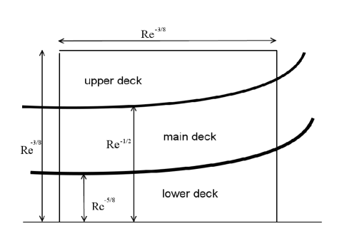
Figure 1: Sketch of triple deck region in the vicinity of heating element.

In addition, the equations on the lower deck are supplied by boundary and initial conditions, which are formulated below, and also by an interaction condition which not only connects functions of lower deck to those of upper deck, but also provides influence of the right boundary of the whole flow region to the behavior of functions inside the region. It implies that the set of equations in the lower deck can not be viewed as that of parabolic type and gains, in a sense, the property of ellipticity.

The lower deck is the most essential part of the hierarchy for the pressure gradient presented in equations for all decks is not fixed but becomes self-induced, i.e., varies on account of displacement thickness of the boundary layer to the outer inviscid flow, and the main contribution to the variation of the pressure is furnished by the very lower deck, while the main deck(the main part of the boundary layer) remains passive and merely conveys perturbations from the lower deck to the outer flow. The indicated scheme enables to construct solutions of equations in the lower deck with self-induced pressure gradient and thus provides interaction between lower and upper decks.

We give the formulation of the set of equations for lower deck, further called the viscous sublayer, referring to (Koroteev & Lipatov, 2009, 2011) for details of derivation.

The set of equations for the viscous sublayer has the form

$$\frac{\partial u_{b}}{\partial x_{b}}+\frac{\partial v_{b}}{\partial y_{b}}=0,$$

$$u_{b}\frac{\partial u_{b}}{\partial x_{b}}+v_{b}\frac{\partial u_{b}}{\partial y_{b}}+T_{b}\frac{\partial p_{b}}{\partial x_{b}}=\frac{\partial^{2}u_{b}}{\partial y_{b}^{2}},$$ (1)

$$u_{b}\frac{\partial T_{b}}{\partial x_{b}}+v_{b}\frac{\partial T_{b}}{\partial y_{b}}=\frac{\partial^{2}T_{b}}{\partial y_{b}^{2}}.$$

Here $u_{b},v_{b}$ are longitudal and vertical components of velocity in the sublayer, $T_{b}$ - the perturbation of temperature, $p_{b}(x)$ is the pressure which only depends on $x$ and consequently is constant through the decks.

The system is supplied by the following boundary conditions. On the surface the non-slip conditions are stated

$$u_{b}(x_{b},0)=v_{b}(x_{b},0)=0.$$ (2)

We prescribe a temperature profile on he surface:

$$T_{b}(x_{b},0)=T_{w}(x_{b}).$$ (3)

The boundary condition at significant distance from the surface is presented as follows

$$u_{b}\to y_{b}+\mathcal{A}(x_{b}),\quad\mathcal{A}_{1}(x_{b})=\int_{0}^{+\infty}(1-T_{b})d\eta+\mathcal{A}(x_{b}),$$

$$\quad T_{b}(x,\infty)\to 1,y_{b}\to\infty.$$ (4)

The function $\mathcal{A}(x_{b})$ is a standard displacement by means of which the problems of interaction without heat perturbations are formulated(Jobe & Burgraff, 1974; Sychev et al., 1998). Local perturbations of the temperature generate an effective local hump(Lipatov, 2006) and additionally contribute to the boundary condition for $y_{b}\to+\infty$, which is expressed by means of a function $\mathcal{A}_{1}(x_{b})$. The temprature perturbations vanish far from the location of the heated region and $\mathcal{A}(x_{b})$ tends to $\mathcal{A}_{1}(x_{b})$ as it follows from the above condition.

The conditions which relate the displacement thickness with the longitudal velocity are supplied by the interaction condition, which, in turn, relates the displacement thickness with the pressure which provides the interaction of the viscous sublayer with the outer inviscid flow.

The condition of interaction differs for subsonic and supersonic flows. We do not give its derivation for this question was many times discussed in literature (Stewartson, 1981; Sychev et al., 1998). In part, for the supersonic flow which we study, the condition of interaction has the form

$$p(x_{b})=-B\frac{\partial\mathcal{A}_{1}(x_{b})}{\partial x_{b}}.$$ (5)

Here $B$ is a constant which allows to consider different regimes of interaction. In our case $B\sim 1$ which corresponds to the regime of free interaction.

3 Numerical solution of boundary problem

The numerical solution the problem (1-5) is constructed on the premise of the method suggested in (Ruban, 1976), the detailed description of which can be found in (Sychev et al., 1998). The method was originally employed for computations of subsonic problems but can be also utilized for supersonic flows. Supplying the equation for temperature we thus give but a short sketch of the procedure, paying attention to necessary modifications of the numerical method.

In the first place the boundary problem described in the previous section is reduced to that for vorticity $\tau=\partial u/\partial y_{b}$. This is carried out by differentiating the momentum equation wrt. $y_{b}$ and taking into account the equation of continuity. Then the system becomes

$$u_{b}\frac{\partial\tau}{\partial x_{b}}+v_{b}\frac{\partial\tau}{\partial y_{b}}+\frac{\partial T_{b}}{\partial y_{b}}\frac{\partial p_{b}}{\partial x_{b}}=\frac{\partial^{2}\tau}{\partial y_{b}^{2}},$$

(6)

$$u_{b}\frac{\partial T_{b}}{\partial x_{b}}+v_{b}\frac{\partial T_{b}}{\partial y_{b}}=\frac{\partial^{2}T_{b}}{\partial y_{b}^{2}}.$$

The boundary conditions have the following form

$$\tau\to 1,y_{b}\to+\infty,x_{b}\to-\infty.$$ (7)

Non-slip conditions (2) as well as those for the temperature (3) are retained on the wall.

Next it is easily seen that the momentum equation gives

$$T_{w}(x_{b})\frac{\partial p}{\partial x_{b}}=\frac{\partial\tau}{\partial y_{b}},\quad y_{b}=0.$$ (8)

From this equation we obtain using the interaction condition (5)

$$-BT_{w}(x_{b})\frac{\partial^{2}\mathcal{A}_{1}}{\partial x^{2}_{b}}=\frac{\partial\tau}{\partial y_{b}},\quad y_{b}=0.$$ (9)

Localization of the effective hump implies the decay of perturbations downstream, namely

$$p(x_{b})\to 0,\quad x_{b}\to+\infty.$$

The last condition implies, according to (5), that

$$\frac{\partial\mathcal{A}_{1}(x_{b})}{\partial x_{b}}\to 0,\quad x_{b}\to+\infty.$$ (10)

The numerical method provides some freedom in the consecutive evaluations of the functions as the number of relations between them exceeds the number of functions. We describe but one possible realization of the procedure which enables to carry out the computations.

The grid is given by $(x_{j},y_{k})$, $j=1,2\ldots N,k=1,2\ldots M$, with steps $\Delta x,\Delta y$ respectively.

The system (6) is approximated as follows

$$u_{jk}\left(\frac{\partial\tau}{\partial x}\right)^{*}_{jk}+v_{jk}\frac{\tau_{jk+1}-\tau_{jk-1}}{2\Delta y}+p^{\prime}_{jk}\frac{T_{jk+1}-T_{jk-1}}{2\Delta y}=$$

$$=\frac{\tau_{jk-1}-2\tau_{jk}+\tau_{jk+1}}{\Delta y^{2}},$$

(11)

$$u_{jk}\frac{T_{j+1k}-T_{jk}}{\Delta x}+v_{jk}\frac{T_{jk+1}-T_{jk-1}}{2\Delta y}+\frac{T_{jk-1}-2T_{jk}+T_{jk+1}}{\Delta y^{2}}$$

where

$$\left(\frac{\partial\tau}{\partial x}\right)^{*}_{jk}=\left\{\begin{array}[]{ll}\frac{\tau_{jk}-\tau_{j-1k}}{\Delta x},&u_{jk}\geq 0\\[2.0pt] \frac{\tau_{j+1k}-\tau_{jk}}{\Delta x},&u_{jk}<0\end{array}\right.$$ (12)

We thus notice that depending on the sign of the longitudal velocity different templates are employed. This is quite a famous method for securing static stability of the difference scheme (Roache, 1972). Derivatives wrt. $x$ can be approximated using the values in three points (Sychev et al., 1998). However our computations show that this alteration does not produce noticeable effect in accuracy, at least for supersonic flows. Therefore we employed tow-point templates.

The solution is constructed by iterations with respect to $\mathcal{A}_{1}(x_{b})$ using under relaxation (Sychev et al., 1998). Let the approximation of $\mathcal{A}_{1}^{n}(x_{b})$ is known on some step of the iteration procedure. At each line $x=x_{j}$ the first equation of (11) is reduced to a linear set of algebraic equations with a tridiagonal matrix and solved consecutively from the bottom to the top of the grid with the boundary conditions (9) and (7) and then the equation for temperature (11) is solved with the boundary conditions (3), (4). Then the computations are transferred to the next line. It allows to fulfill computations of vorticity and temperature in the whole 2D region.

The right boundary attained, the functions $u_{jk},v_{jk}$ as well as $\hat{\mathcal{A}}_{1}(x_{b})$ are recomputed on the current iteration in the whole field and the new approximation for $\mathcal{A}_{1}(x_{b})$ is evaluated from the relaxation

$$\mathcal{A}_{1}^{n+1}=(1-r)\mathcal{A}_{1}^{n}+r\hat{\mathcal{A}}_{1}(x_{b}),$$

where $r$ is a relaxation parameter. In problems of interaction theory it usually turns out that convergence of iterations is strongly sensitive to the values of this parameter(Smith, 1977; Sychev et al., 1998). The problem under consideration is not an exception. In fig. 2

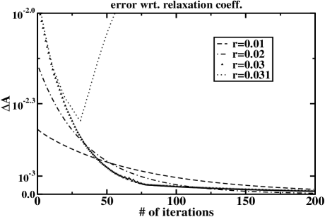
Figure 2: Behavior or error $\Delta A$ in consecutive iterations for various values of the relaxation parameter $r$.

the errors $\Delta A=\mathcal{A}^{n+1}-\mathcal{A}^{n}$ are presented for several values of the relaxation parameter. It is noticed that convergence, which exists for $r=0.02$, vanishes even for $r=0.031$. In our computations we took $r=0.02$, the value which was found empirically and which yields an estimate of the upper boundary of some interval of convergence.

4 Results of computations

The key functions to evaluate are distributions of pressure and shear stress on the surface. As we said, the self-induced pressure is constant through the layers and thus its values remain valid in the inviscid flow for the fixed $x_{b}$. The shear stress in turn can be thought of as a general function characterizing forces in the flow.

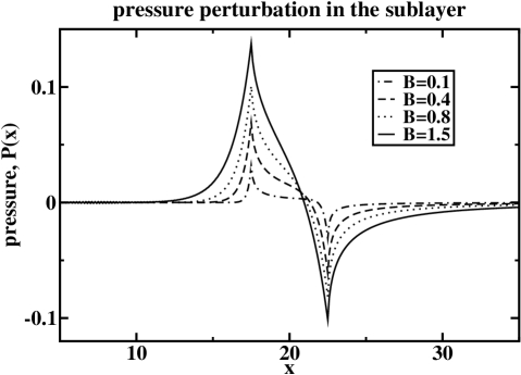
Figure 3: Pressure in the viscous sublayer obtained from the numerical solution of the problem. Small $B$ decline pressure perturbations even if $\Delta T$ is not small.

In fig. 3 it is exhibited the pressure in the viscous sublayer for heat humps, of a somewhat artificial form, which are given by

$$T_{w}(x_{b})=\left\{\begin{array}[]{ll}1+h,&\left|x_{b}\right|\leq a/2\\[2.0pt] 1,&\left|x_{b}\right|>a/2\end{array}\right.$$ (13)

Here $h$ the perturbation of the temperature and $a$ the size of the heated region. For computations we take $h=0.3-0.4$.

This form of temperature distribution is simpler for analytic study and in the same time enables to represent adequately qualitative behavior of functions in the flow. The results are presented for various $B$. It is noticed that the pressure perturbations decrease for small $B$ even if $\Delta T\sim O(1)$. This situation corresponds to compensated interaction regime which is discussed elsewhere.

The comparison of computations for nonlinear and linear cases, the latter corresponding to small temperature perturbations, is represented in fig. 4. The difference is especially noticeable in the transient region and downstream which are not quite adequately approximated by the linear theory.

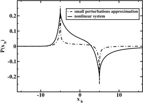
Figure 4: Pressure in the viscous sublayer obtained from the numerical solution of the problem compared to linear solution which corresponds to small temperature perturbations and was presented in (Koroteev & Lipatov, 2009). For both cases the heated region is determined by (13) with the size $10$.

The flow moves from the left to the right. When approaching the heated region the positive pressue gradient produces aditional deceleration of the flow, thus delaying possible laminar-turbulent transition. Note that there are two possible separation points in the flow, namely boundaries of the heated region upstream and downstream (fig. 5). They have to be controlled if the separation is not desirable. In the transient region between these points and over the heating element the flow accelerates affected by the negative pressure gradient which simultaniously increases the shear stress. Finally perturbations of the pressur decay Behind the heated region and the flow againg slows down. The parameter $B$ from (9) influences the amplitude of pressure perturbations. As we mentioned before the regime of free interaction implies $B\sim 1$.

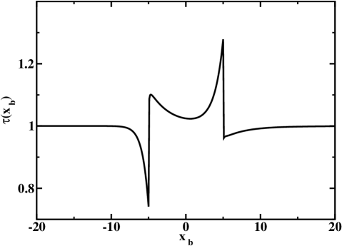
Figure 5: Shear stress in the boundary layer.

5 Conclusions

The problem whose solution is presented in this paper presumabily can essentially contribute to possibility of control of boundary layer and general understading of influence of thermal perturbations to both subsonic and supersonic flows. Possible closest developements of this work imply generalization of the obtained solutions to three dimensional case which is of course of more interest for applications. From the other hand, another direction would be the generalization of these results to nonstationary flow where it is essential to study nonlinear perturbations and their propagation. Both these problems are under consideration and will be published elsewhere.

References

- Bogolepov & Neiland (1971) Bogolepov, V. V. & Neiland, V. Y. 1971 Supersonic flow over small humps located on the surface. Transactions of TsAGI 1363.
- Bogolepov & Neiland (1976) Bogolepov, V. V. & Neiland, V. Y. 1976 On local perturbations of viscous supersonic flows. In Aeromechanics, pp. 104–118. Nauka, in Russian.
- Jobe & Burgraff (1974) Jobe, C. E. & Burgraff, O. R. 1974 The numerical solution of the asymptotitc equations of trailing edge flow. Proc. R. Soc. Lond. A 340, 91–111.
- Koroteev & Lipatov (2009) Koroteev, M. V. & Lipatov, I. I. 2009 Supersonic boundary layer in regions with small temperature perturbations on the wall. SIAM J. App. Math. 70(4), 1139–1156.
- Koroteev & Lipatov (2011) Koroteev, M. V. & Lipatov, I. I. 2011 Stationary subsonic boundary layer in the regions of local heating of surface. App. Math. Mech. Accepted, arXiv:0812.2513.
- Lipatov (2006) Lipatov, I. I. 2006 Disturbed boundary layer flow with local time-dependent surface heating. Fluid Dyn. 41(5), 55–65.
- Messiter (1970) Messiter, A. F. 1970 Boundary layer near the trailing edge of a flat plane. SIAM J. Appl. Math. 18, #1, 241–257.
- Neiland (1969) Neiland, V. Y. 1969 To the theory of laminar separation of boundary layer in supersonic flow. Izv. Acad. Nauk SSSR, Mech. Zhid. Gasa 4, 53–57, in Russian.
- Roache (1972) Roache, P. J. 1972 Computational fluid dynamics. Hermosa Pub.
- Ruban (1976) Ruban, A. I. 1976 To the theory of laminar separation of fluid from the point of zero turn of solid surface. Trans. TsAGI 7(4), 18–28, in Russian.
- Smith (1974) Smith, F. T. 1974 Laminar flow over a small hump on a flat plate. J. Fluid Mech. 57(4), 803–824.
- Smith (1977) Smith, F. T. 1977 The laminar separation of an incompressible fluid streaming past a smooth surface. Proc. Roy. Soc. London A 356(1687), 443–463.
- Stewartson (1981) Stewartson, K. 1981 D’alembert’s paradox. SIAM Review 23(3), 308–343.
- Stewartson & Williams (1969) Stewartson, K. & Williams, P. G. 1969 Self-induced separation. Proc. Roy. Soc. Ser. A, 312, 181–206.
- Sychev et al. (1998) Sychev, V. V., Ruban, A. I., Sychev, Vic. V. & Korolev, G. I. 1998 Asymptotitc theory of separated flows. Cambridge. Univ. Press.