Efficient Detection of Hot Span in Information Diffusion from Observation

Abstract

We addressed the problem of detecting the change in behavior of information diffusion from a small amount of observation data, where the behavior changes were assumed to be effectively reflected in changes in the diffusion parameter value. The problem is to detect where in time and how long this change persisted and how big this change is. We solved this problem by searching the change pattern that maximizes the likelihood of generating the observed diffusion sequences. The naive learning algorithm has to iteratively update the patten boundaries, each requiring optimization of diffusion parameters by the EM algorithm, and is very inefficient. We devised a very efficient search algorithm using the derivative of likelihood which avoids parameter value optimization during the search. The results tested using three real world network structures confirmed that the algorithm can efficiently identify the correct change pattern. We further compared our algorithm with the naive method that finds the best combination of change boundaries by an exhaustive search through a set of randomly selected boundary candidates, and showed that the proposed algorithm far outperforms the native method both in terms of accuracy and computation time.

1 Introduction

Social networking is now an important part of our daily lives, and our behavioral patterns are substantially affected by the communication through these networks Newman et al. (2002); Newman (2003); Gruhl et al. (2004); Domingos (2005); Leskovec et al. (2006). It has been shown that a social network has many interesting properties, e.g. power law for node degree distribution, large clustering coefficient, positive degree correlation, etc. Wasserman and Faust (1994), which affect how the information actually diffuses through the network, and researchers have devised several important measures to characterize these features based on the topology/structure of the network Wasserman and Faust (1994); Bonacichi (1987); Katz (1953). These measures, called centrality measures, are expected to be used to identify important nodes in the network. However, recent studies have shown that it is important to consider the diffusion mechanism explicitly and the measures based on network structure alone are not enough to identify the important nodes Kimura et al. (2009, 2010a).

Information diffusion is modeled typically by a probabilistic model. Most representative and fundamental ones are independent cascade (IC) model Goldenberg et al. (2001); Kempe et al. (2003), linear threshold (LT) model Watts (2002); Watts and Dodds (2007) and their extensions that include incorporating asynchronous time delay Saito et al. (2009). Explicit use of these models to solve such problems as the influence maximization problem Kempe et al. (2003); Kimura et al. (2010a) and the contamination minimization problem Kimura et al. (2009) clearly shows the advantage of the model. The identified influential nodes and links are considerably different from the ones identified by the centrality measures. However, use of these models brings in yet another difficulty. They have parameters that need be specified in advance, e.g. diffusion probabilities for the IC model, and weights for the LT model, and their true values are not known in practice. A series of studies by Saito et al. (2009, 2010) have shown one way of solving this problem in which they used a limited amount of observed information diffusion data and trained/learned the model such that the likelihood of generating the observed data by the model is maximized.

This paper is in the same line of these studies, but addresses a different aspect of information diffusion. Almost all of the work so far assumed that the model is stationary. We note that our behavior is affected not only by the behaviour of our neighbors but also by other external factors. The model only accounts for the interaction with neighbors. The problem we address here is to detect the change of the model from a limited amount of observed information diffusion data. If this is possible, we can infer that something unusual happened during a particular period of time by simply analyzing the limited amount of data.

This is in some sense the same, in the spirit, with the work by Kleinberg (2002) and  Swan and Allan (2000). They noted a huge volume of the data stream, tried to organize it and extract structures behind it. This is done in a retrospective framework, i.e. assuming that there is a flood of abundant data already and there is a strong need to understand it. Our aim is not exactly the same as theirs. We are interested in detecting changes which is hidden in the data. We also follow the same retrospective approach, i.e. we are not predicting the future, but we are trying to understand the phenomena that happened in the past. There are many factors that bring in changes and the model cannot accommodate all of them. We formalize this as the unknown changes in the diffusion parameter value, and we reduce the problem to that of detecting where in time and how long this change persisted and how big this change is. We call the period where the parameter takes anomalous values as “hot span” and the rest as “normal span”. To make the analysis simple, we limit the diffusion model to the asynchronous independent cascade model (AsIC) Saito et al. (2009) and the form of change to a rect-linear one, that is, the diffusion parameter changes to a new large value, persists for a certain period of time and is restored to the original value and stays the same thereafter . In this simplified setting, detecting the hot span is equivalent to identifying the time window where the parameter value is high and estimating the parameter values both in hot and normal spans.

To this end, we use the same parameter optimization algorithm as in Saito et al. (2009), i.e. the EM algorithm that iteratively updates the values to maximize the model’s likelihood of generating the observed data sequences. The problem here is more difficult because it has another loop to search for the hot span on top of the above loop. The naive learning algorithm has to iteratively update the patten boundaries requiring the parameter value optimization for each combination, which is a very inefficient procedure. Our main contribution is that we devised a very efficient general search algorithm which avoids the inner loop optimization by using the information of the first order derivative of the likelihood with respect to the diffusion parameters. We tested its performance using the structures of three real world networks (blog, Coauthorship and Wikipedia), and confirmed that the algorithm can efficiently identify the hot span correctly as well as the diffusion parameter values. We further compared our algorithm with the naive method that finds the best combination of change boundaries by an exhaustive search from a set of randomly selected boundary candidates, and showed that the proposed algorithm far outperforms the native method both in terms of accuracy and computation time.

2 Information Diffusion Model

The AsIC model we use in this paper incorporates asynchronous time delay into the independent cascade (IC) model which does not account for time-delay, reflecting that each node changes its state asynchronously in reality. We recall the definition of the AsIC model below, in which we consider choosing a delay-time from the exponential distribution for the sake of convenience, but of course other distributions such as power-law and Weibull can be employed.

Let $G=(V,E)$ be a directed graph, where $V$ and $E$ ($\subset V\times V$) are the sets of all the nodes and the links. For any $v\in V$, the set of all the nodes that have links from $v$ is denoted by $F(v)$ $=$ $\{u\in V;\ (v,u)\in E\}$ and the set of all the nodes that have links to $v$ by $B(v)$ $=$ $\{u\in V;\ (u,v)\in E\}$. Each node has one of the two states (active and inactive), and the nodes are called active if they have been influenced. It is assumed that nodes can switch their states only from inactive to active.

The AsIC model has two types of parameters $p_{u,v}$ and $r_{u,v}$ with $0$ $<$ $p_{u,v}$ $<$ $1$ and $r_{u,v}$ $>$ $0$, where $p_{u,v}$ and $r_{u,v}$ are referred to as the diffusion probability through link $(u,v)$ and the time-delay parameter through link $(u,v)$, respectively. The information diffusion process unfolds in continuous-time $t$, and proceeds from a given initial active node in the following way. When a node $u$ becomes active at time $t$, it is given a single chance to activate each currently inactive node $v\in F(u)$. A delay-time $\delta$ is chosen from the exponential distribution with parameter $r_{u,v}$. The node $u$ attempts to activate the node $v$ if $v$ has not been activated by time $t+\delta$, and succeeds with probability $p_{u,v}$. If $u$ succeed, $v$ will become active at time $t+\delta$. The information diffusion process terminates if no more activations are possible.

3 Problem Setting

We address the hot span detection problem. In this problem, we assume that some change has happened in the way the information diffuses, and we observe the diffusion sequences of a certain topic in which the change is embedded, and consider detecting where in time and how long this change persisted and how big this change is. We place a constraint that $p_{u,v}$ and $r_{u,v}$ do not depend on link $(u,v)$, i.e. $p_{u,v}=p$, $r_{u,v}=r$ ($\forall(u,v)\in E$), which should be acceptable noting that we can naturally assume that people behave quite similarly when talking about the same topic (see Section 6).

Let $[T_{1},T_{2}]$ denote the hot span of the diffusion of a topic, and let $p_{1}$ and $p_{2}$ denote the values of the diffusion probability of the AsIC model for the normal span and the hot span, respectively. Note that $p_{1}<p_{2}$. A diffusion result of the topic is represented as a set of pairs of active nodes and their activation times; i.e. $\{(u,t_{u}),(v,t_{v}),\cdots\}$. We consider a diffusion result $D$ that is generated by the AsIC model with $p_{1}$ for the period $[0,T_{1})$, $p_{2}$ for the period $[T_{1},T_{2}]$ and $p_{1}$ for the period $(T_{2},\infty)$, where the time-delay parameter does not change and takes the same value $r$ for the entire period $[0,\infty)$. We refer to the set $D$ as a diffusion result with a hot span. The problem is reduced to detecting $[T_{1},T_{2}]$ and estimating $p_{1}$ and $p_{2}$ from the observed diffusion results. Extensions of this problem setting is discussed later (see Section6).

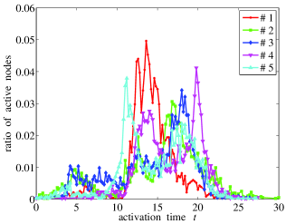
Figure 1: Information diffusion in the blog network with a hot span for the AsIC model.

Figure 1 shows examples of diffusion samples with a hot span based on the AsIC model, where the parameters are set at $p_{1}=0.1$, $p_{2}=0.3$, $r=1.0$, $T_{1}=10$ and $T_{2}=20$. The network used is the blog network described later in Subsection 5.1. We plotted the ratio of active nodes (the number of active nodes at a time step $t$ divided by the number of total active nodes over the whole time span) for five independent simulations, each from a randomly chosen initial source node at time $t=0$. We can clearly see bursty activities around the hot span $[T_{1}=10,T_{2}=20]$. However, each curve behaves differently, i.e., some has its bursty activities only in the first half, some other has them only in the last half, and yet some other has two peaks during the hot span. This means that it is quite difficult to accurately detect the true hot span from only a single diffusion sample. Methods that use only the observed bursty activities, including those proposed by Swan and Allan (2000) and Kleinberg (2002) would not work. We believe that an explicit use of underlying diffusion model is essential to solve this problem. It is crucially important to detect the hot span precisely in order to identify the external factors which caused the behavioral changes.

4 Hot Span Detection Methods

Let $\{D_{m};\ m=1,\cdots,M\}$ be a set of $M$ independent information diffusion results, where $D_{m}=\{(u,t_{m,u}),\ (v,t_{m,v}),\ \cdots\}$. Each $D_{m}$ is associated with the observed initial time $\phi_{m}=\min\{t_{m,v};\ (v,t_{m,v})\in D_{m}\}$, and the observed final time $\Phi_{m}\geq\max\{t_{m,v};\ (v,t_{m,v})\in D_{m}\}$. We express our observation data by ${\cal D}_{M}=\{(D_{m},\Phi_{m});\ m=1,\cdots,M\}$. For any $t\in[\phi_{m},\Phi_{m}]$, we set $C_{m}(t)=\{v;\ (v,t_{m,v})\in D_{m},\ t_{m,v}<t\}$. Namely, $C_{m}(t)$ is the set of active nodes before time $t$ in the $m$th diffusion result. For convenience sake, we use $C_{m}$ as referring to the set of all the active nodes in the $m$th diffusion result.

4.1 Parameter Learning Framework

The following logarithmic likelihood function ${\cal L}({\cal D}_{M};p,r)$ has been derived to estimate the values of $p$ and $r$ from ${\cal D}_{M}$ for the AsIC model in case there is no hot span Saito et al. (2009),

$${\cal L}({\cal D}_{M};p,r) = \sum_{m=1}^{M}{\cal L}((D_{m},\Phi_{m});p,r)$$ (1)

$$= \sum_{m=1}^{M}\sum_{v\in C_{m}}\left(\log h_{m,v}+\sum_{w\in F(v)\setminus C_{m}}\log g_{m,v,w}\right),$$

where $h_{m,v}$ is the probability density that a node $v$ $\in D_{m}$ with $t_{m,v}>0$ is activated at a time $t_{m,v}$, and $g_{m,v,w}$ is the probability that a node $w$ is not activated by a node $v$ within $[\phi_{m},\Phi_{m}]$, where there exists a link $(v,w)\in E$ and $v\in C_{m}$. The values of $p$ and $r$ can be stably obtained by maximizing Eq. (1) using the EM algorithm Saito et al. (2009).

The following parameter switching applies for a hot span $S=[T_{1},T_{2}]$ where ${\cal N}_{m}$ and ${\cal H}_{m}$ denote the sets of active nodes in the $m$-th diffusion result during the normal and the hot spans, respectively.

$$p = \left\{\begin{array}[]{ll}p_{1}&\mbox{if~{}$v\in{\cal N}_{m}(S),\ {\cal N}_{m}(S)=C_{m}(T_{1})\cup(C_{m}\setminus C_{m}(T_{2}))$},\\ p_{2}&\mbox{if~{}$v\in{\cal H}_{m}(S),\ {\cal H}_{m}(S)=C_{m}(T_{2})\setminus C_{m}(T_{1})$}.\end{array}\right.$$

Then, an extended objective function ${\cal L}({\cal D}_{M};p_{1},p_{2},r,S)$ can be defined by adequately modifying Eq. (1) under this switching scheme. Clearly, ${\cal L}({\cal D}_{M};p_{1},p_{2},r,S)$ is expected to be maximized by setting $S$ to the true span $S^{*}=[T_{1}^{*},T_{2}^{*}]$ if a substantial amount of data ${\cal D}_{M}$ is available. Thus, our problem is to find the following $\hat{S}$.

$$\hat{S} = \arg\max_{S}{\cal L}({\cal D}_{M};\hat{p}_{1},\hat{p}_{2},\hat{r},S),$$ (3)

where $\hat{p}_{1}$, $\hat{p}_{2}$, and $\hat{r}$ denote the maximum likelihood estimators for a given $S$.

In order to obtain $\hat{S}$, we need to prepare a reasonable set of candidate spans, denoted by ${\cal S}$. One way of doing so is to construct ${\cal S}$ by considering all pairs of observed activation time points: ${\cal S}=\{S=[t_{1},t_{2}]:t_{1}<t_{2},t_{1}\in{\cal T},t_{2}\in{\cal T}\}$, where ${\cal T}=\{t_{1},\cdots,t_{N}\}$ is a set of activation time points in ${\cal D}_{M}$.

4.2 Naive Method

Now we describe the naive method, which has two iterative loops. In the inner loop we first obtain the maximum likelihood estimators, $\hat{p}_{1}$, $\hat{p}_{2}$, and $\hat{r}$, for each candidate $S$ by maximizing ${\cal L}({\cal D}_{M};p_{1},p_{2},r,S)$ using the EM algorithm. In the outer loop we select the optimal $\hat{S}$ which gives the largest ${\cal L}({\cal D}_{M};\hat{p}_{1},\hat{p}_{2},\hat{r},S)$ value. However, this can be extremely inefficient when $N$ is large. To make it work with a reasonable computational cost, we restrict the number of candidate time points $N$ to a smaller value $K$ by selecting $K$ points from ${\cal T}$, i.e., we construct ${\cal S}_{K}=\{S=[t_{1},t_{2}]:t_{1}<t_{2},t_{1}\in{\cal T}_{k},t_{2}\in{\cal T}_{K}\}$, where ${\cal T}_{K}=\{t_{1},\cdots,t_{K}\}$. Note that $|{\cal S}_{K}|=K(K-1)/2$, which is large when $K$ is large.

4.3 Proposed Method

The naive method should be able to detect the hot span with a reasonable accuracy when $K$ is set large at the expense of the computational cost, but the accuracy becomes poorer when $K$ is set smaller to reduce the computational load. We propose a novel detection method which alleviates this problem and can efficiently and stably detect a hot span from ${\cal D}_{M}$.

We first obtain $\hat{p}$, and $\hat{r}$, based on the original objective function of Eq. (1), and focus on its first-order derivative with respect to $p$ for each node at each individual activation time. Let $p_{u,v}$ be the diffusion parameter from a node $u$ to a node $v$. The following formula holds for the maximum likelihood estimators due to the uniform parameter setting of Eq. (1) and the locally optimal condition.

$$\frac{\partial{\cal L}({\cal D}_{M};\hat{p},\hat{r})}{\partial p} = \sum_{(u,v)\in E}\frac{\partial{\cal L}({\cal D}_{M};\hat{p},\hat{r})}{\partial p_{u,v}}\ =\ 0.$$ (4)

Consider the following partial sum for a given $S=[T_{1},T_{2}]$.

$${\cal G}(S) = \sum_{m=1}^{M}\sum_{(u,v)\in E,u\in{\cal H}_{m}(S)}\frac{\partial{\cal L}((D_{m},\Phi_{m});\hat{p},\hat{r})}{\partial p_{u,v}}.$$ (5)

Clearly, ${\cal G}(S)$ should be sufficiently large if $S\approx S^{*}$ due to our problem setting, which leads to $p_{2}>\hat{p}>p_{1}$. Thus, the hot span $S^{*}$ can be estimated by searching for ${\hat{S}}$ that maximizes ${\cal G}(S)$.

$${\hat{S}} = \arg\max_{S\in{\cal S}}{\cal G}(S).$$ (6)

The nice thing here is that we can incrementally calculate ${\cal G}(S)$ by Eq. (7), where ${\cal T}=\{t_{1},\cdots,t_{N}\}$ and $t_{i}<t_{j}$ if $i<j$.

$${\cal G}([t_{i},t_{j+1}]) = {\cal G}([t_{i},t_{j}])+\sum_{m=1}^{M}\sum_{\stackrel{{\scriptstyle\scriptstyle(u,v)\in E}}{{u\in C_{m}(t_{j+1})\setminus C_{m}(t_{j})}}}\frac{\partial{\cal L}((D_{m},\Phi_{m});\hat{p},\hat{r})}{\partial p_{u,v}}.$$ (7)

The computational cost for examining each candidate span is much smaller than the naive method described above. Thus, we can use all the pairs to construct ${\cal S}$. We summarize our proposed method below.

1.

Maximize ${\cal L}({\cal D}_{M};p,r)$ by using the EM algorithm.

2.

Construct ${\cal T}$ and ${\cal S}$.

3.

Detect $\hat{S}$ by Eq. (6) and output $\hat{S}$.

4.

Maximize ${\cal L}({\cal D}_{M};p_{1},p_{2},r,\hat{S})$ by using the EM algorithm, and output $\hat{p}_{1}$, $\hat{p}_{2}$, and $\hat{r}$.

Here note that the proposed method requires maximization by using the EM algorithm only twice.

5 Experiments

We experimentally investigated how accurately the proposed method can estimate both the hot span and the diffusion probabilities in the hot and normal spans, as well as its efficiency, by comparing it with the naive method using three real world networks. We used three different values for $K$, i.e., $K=5$, $10$, and $20$ for the naive method.

The derivation assumed that there are multiple observed data sequences, but in the experiments we chose to learn from a single sequence, i.e., $M=1$, which is the most difficult situation.

5.1 Datasets

The three data are all bidirectionally connected networks. The first one is a trackback network of Japanese blogs used in Kimura et al. (2009), which has $12,047$ nodes and $79,920$ directed links (the blog network). The second one is a coauthorship network used in Palla et al. (2005), which has $12,357$ nodes and $38,896$ directed links (the Coauthorship network). The last one is a network of people that was derived from the “list of people” within Japanese Wikipedia, used in Kimura et al. (2009), and has $9,481$ nodes and $245,044$ directed links (the Wikipedia network).

For these networks, we generated diffusion samples with a hot span using the AsIC model. According to Kempe et al. (2003), we set the diffusion probability for the normal span, $p_{1}$, to be a value smaller than $1/{\bar{d}}$, where $\bar{d}$ is the mean out-degree of a network, and set the diffusion probability for the hot span, $p_{2}$, to be three times larger than $p_{1}$. Thus, $p_{1}$ and $p_{2}$ are $0.1$ and $0.3$ for the blog network, $0.2$ and $0.6$ for the Coauthorship network, and $0.02$ and $0.06$ for the Wikipedia network, respectively. We fixed the time-delay parameter at 1 ($r=1$) for all the networks because changing $r$ works only for scaling the time axis of the diffusion results. We set the hot span to $[T_{1}=10,T_{2}=20]$ based on the observation on the preliminary experiments. In all we generated five information diffusion samples using these parameter values for each network, randomly selecting an initial active node for each diffusion sample.

5.2 Results

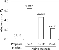
(a) Blog

(b) Coauthorship

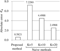
(c) Wikipedia

Figure 2: Comparison in accuracies of the estimated hot span

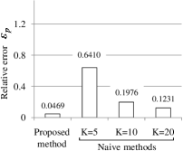
(a) Blog

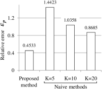
(b) Coauthorship

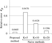
(c) Wikipedia

Figure 3: Comparison in accuracies of the estimated diffusion probability

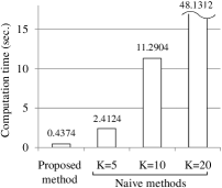
(a) Blog

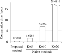
(b) Coauthorship

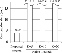
(c) Wikipedia

Figure 4: Comparison in computation time

We compared the proposed method with the naive method in terms of 1) the accuracy of the estimated hot span ${\hat{\cal S}}=[\hat{T}_{1},\hat{T}_{2}]$, 2) the accuracy of the diffusion probabilities $p_{1}$ (for the normal span) and $p_{2}$ (for the hot span), and 3) the computation time. Both the proposed and the naive methods were tested to each diffusion sample mentioned above, and the results were averaged over the five independent trials for each network.

Figure 4 shows the accuracy for ${\hat{\cal S}}$ in the absolute error ${\cal E}_{s}=|\hat{T}_{1}-T_{1}|+|\hat{T}_{2}-T_{2}|$. We see that the proposed method achieves a good accuracy, much better than the naive method for every network. As expected, ${\cal E}_{s}$ for the naive method decreases as $K$ becomes larger. But, even in the best case ($K=20$), its average error is about 3 to 10 times larger than that of the proposed method. Figure 4 shows the accuracy of $p_{1}$ and $p_{2}$ in the relative error ${\cal E}_{p}=|\hat{p}_{1}-p_{1}|/p_{1}+|\hat{p}_{2}-p_{2}|/p_{2}$. Here again, the average relative error for the naive method decreases as $K$ becomes larger. However, even in the best case ($K=20$), it is about 2 to 3 times larger than that of the proposed method. We note that the average errors for the Coauthorship network are relatively large. This is because the number of active nodes within the normal span was relatively small for this network. Figure 4 shows the computation time. It is clear that the proposed method is much faster than the naive method. The significant difference is attributed to the difference in the number of runs of the EM algorithm. The proposed method executes the EM algorithm only twice: steps 1 and 4 in the algorithm (see Section 4.3). On the other hand, the naive method has to execute the EM algorithm once for every single candidate span $S\in{\cal S}_{K}$ which is $|{\cal S}_{K}|=K(K-1)/2$ times (see Section 4.2). Indeed, the computation time of the naive method for $K=5$ is about 5 times larger for every network, which is consistent with $|{\cal S}_{K}|=10$. This relation roughly holds also for the other two cases ($K=10$ and $K=20$). This means that even if the naive method could achieve a good accuracy by setting $K$ to a sufficiently large value, it would require unacceptable computation time for such a large $K$.

In summary, we can say that the proposed method can detect and estimate the hot span and diffusion probabilities much more accurately and efficiently compared with the naive method. Here we mention that we could obtain much better results by using more than one diffusion sequence, say $M=5$, but we have to omit the details due to space limitations.

6 Discussion

We placed a simplifying constraint that the parameters $p_{u,v}$ and $r_{u,v}$ are link independent, i.e. $p_{u,v}=p$, $r_{u,v}=r$ ($\forall(u,v)\in E$), by focusing on single topic diffusion sequences. Saito et al. (2009, 2010) gave some evidences for this assumption. They examined $7,356$ diffusion sequences for a real blogroll network containing $52,525$ bloggers and $115,552$ blogroll links, and experimentally confirmed that $p$ and $r$ that were learned from different diffusion sequences belonging to the same topic were quite similar for most of the topics. This observation naturally suggests that people behave quite similarly for the same topic.

In this paper, we considered AsIC model, but it is straightforward to apply the same technique to AsLT model Saito et al. (2010) and to their SIS versions in which each node is allowed to be activated multiple times. The same idea can naturally be applied to opinion formation model, e.g. value-weighted voter model Kimura et al. (2010b).

The change pattern considered here is the simplest one. We can assume a more intricate problem setting such that both $p$ and $r$ change for multiple distinct hot spans and the shape of change pattern $p$ is not necessarily rect-linear. One possible extension is to approximate the pattern of any shape by $J$ pairs of time interval each with its corresponding $p_{j}$, i.e., $Z_{J}=\{([t_{j-1},t_{j}],p_{j});\ j=1,\cdots J\}\ (t_{0}=0,t_{J}=\infty)$ and use a divide-and-conquer type greedy recursive partitioning, still employing the derivative of the likelihood function ${\cal G}$ as the main measure for search. More specifically, we first initialize $Z_{1}=\{([0,\infty),\hat{p}_{1})\}$ where $\hat{p}_{1}$ is the maximum likelihood estimator, and search for the first change time point $t_{1}$, which we expect to be the most distinguished one, by maximizing $|{\cal G}([t,\infty),\hat{p}_{1})|$. We recursively perform this operation $J$ times by fixing the previously determined change points. When to stop can be determined by a statistical criterion such as AIC or MDL. This algorithm requires parameter optimization $J$ times. Figure 5 is one of the preliminary results obtained for two distinct rect-linear patterns using five sequences ($M=5$) in case of the blog network. MDL is used as the stopping criterion. The change pattern of $p$ is almost perfectly detected with respect to both $p_{j}$ and $t_{j}$ ($J=5$).

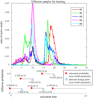
Figure 5: Information diffusion in the blog network with two hot spans for the AsIC model.

7 Conclusion

In this paper, we addressed the problem of detecting the change in behavior of information diffusion from a limited amount of observed diffusion sequences in a retrospective setting, assuming that the diffusion follows the asynchronous independent cascade (AsIC) model. We defined the “hot span” as the period during which the diffusion probability is changed to a relatively high value compared with the other periods (called the normal spans). A naive method to detect such a hot span would have to iteratively update the candidate hot span boundaries, each requiring parameter optimization such that the likelihood function is maximized. This is very inefficient and totally unacceptable. We developed a novel and general framework that avoids the inner loop optimization during search by making use of the first derivative of the likelihood function. It needs to optimize the parameter values only twice by the iterative updating algorithm (EM algorithm), which reduces the computation times by 5 to 100 times, and is very efficient. We compared the proposed method with the naive method that considers only the randomly selected boundary candidates, by applying both the methods (the proposed and the naive) to information diffusion samples generated by simulation from three real world large networks, and confirmed that the proposed method far outperforms the naive method both in terms of accuracy and efficiency. Although we assumed a very simplified problem setting in this paper, the proposed method can be easily extended to solve more intricate problems. We showed one possible direction and the preliminary results obtained for two rect-linear shape hot spans was very promising. Our immediate future work is to evaluate our method using real world information diffusion samples with hot spans, as well as to deal with spatio-temporal hot span detection problems using more appropriate stochastic models under a similar problem solving framework.

References

- Bonacichi [1987] P. Bonacichi. Power and centrality: A family of measures. Amer. J. Sociol., 92:1170–1182, 1987.
- Domingos [2005] P. Domingos. Mining social networks for viral marketing. IEEE Intell. Syst., 20:80–82, 2005.
- Goldenberg et al. [2001] J. Goldenberg, B. Libai, and E. Muller. Talk of the network: A complex systems look at the underlying process of word-of-mouth. Market. Lett., 12:211–223, 2001.
- Gruhl et al. [2004] D. Gruhl, R. Guha, D. Liben-Nowell, and A. Tomkins. Information diffusion through blogspace. SIGKDD Expl., 6:43–52, 2004.
- Katz [1953] L. Katz. A new status index derived from sociometric analysis. Sociometry, 18:39–43, 1953.
- Kempe et al. [2003] D. Kempe, J. Kleinberg, and E. Tardos. Maximizing the spread of influence through a social network. In KDD 2003, pages 137–146, 2003.
- Kimura et al. [2009] M. Kimura, K. Saito, and H. Motoda. Blocking links to minimize contamination spread in a social network. ACM Trans. Knowl. Discov. Data, 3:9:1–9:23, 2009.
- Kimura et al. [2010a] M. Kimura, K. Saito, R. Nakano, and H. Motoda. Extracting influential nodes on a social network for information diffusion. Data Min. Knowl. Disc., 20:70–97, 2010.
- Kimura et al. [2010b] M. Kimura, K. Saito, K. Ohara, and H. Motoda. Learning to predict opinion share in social networks. In AAAI-10, pages 1364–1370, 2010.
- Kleinberg [2002] J. Kleinberg. Bursty and hierarchical structure in streams. In KDD 2002, pages 91–101, 2002.
- Leskovec et al. [2006] J. Leskovec, L. A. Adamic, and B. A. Huberman. The dynamics of viral marketing. In EC’06, pages 228–237, 2006.
- Newman et al. [2002] M. E. J. Newman, S. Forrest, and J. Balthrop. Email networks and the spread of computer viruses. Phys. Rev. E, 66:035101, 2002.
- Newman [2003] M. E. J. Newman. The structure and function of complex networks. SIAM Rev., 45:167–256, 2003.
- Palla et al. [2005] G. Palla, I. Derényi, I. Farkas, and T. Vicsek. Uncovering the overlapping community structure of complex networks in nature and society. Nature, 435:814–818, 2005.
- Saito et al. [2009] K. Saito, M. Kimura, K. Ohara, and H. Motoda. Learning continuous-time information diffusion model for social behavioral data analysis. In ACML 2009, pages 322–337, 2009.
- Saito et al. [2010] K. Saito, M. Kimura, K. Ohara, and H. Motoda. Selecting information diffusion models over social networks for behavioral analysis. In ECML PKDD 2010, pages 180–195, 2010.
- Swan and Allan [2000] R. Swan and J. Allan. Automatic generation of overview timelines. In SIGIR 2000, pages 49–56, 2000.
- Wasserman and Faust [1994] S. Wasserman and K. Faust. Social network analysis. Cambridge Univ. Press, Cambridge, UK, 1994.
- Watts and Dodds [2007] D. J. Watts and P. S. Dodds. Influence, networks, and public opinion formation. J. Consum. Res., 34:441–458, 2007.
- Watts [2002] D. J. Watts. A simple model of global cascades on random networks. PNAS, 99:5766–5771, 2002.