IPMU-11-0171

On 6d $\mathcal{N}=(2,0)$ theory compactified
on a Riemann surface with finite area

Davide Gaiotto¹, Gregory W. Moore² and Yuji Tachikawa³

¹ School of Natural Sciences, Institute for Advanced Study,

Princeton, NJ 08504, USA

² NHETC and Department of Physics and Astronomy, Rutgers University,

Piscataway, NJ 08855, USA

³ IPMU, University of Tokyo, Kashiwa, Chiba 277-8583, Japan

abstract

We study 6d $\mathcal{N}=(2,0)$ theory of type $\mathrm{SU}(N)$ compactified on Riemann surfaces with finite area, including spheres with fewer than three punctures. The Higgs branch, whose metric is inversely proportional to the total area of the Riemann surface, is discussed in detail. We show that the zero-area limit, which gives us a genuine 4d theory, can involve a Wigner-İnönü contraction of global symmetries of the six-dimensional theory. We show how this explains why subgroups of $SU(N)$ can appear as the gauge group in the 4d limit. As a by-product we suggest that half-BPS codimension-two defects in the six-dimensional $(2,0)$ theory have an operator product expansion whose operator product coefficients are four-dimensional field theories.

1 Introduction

In the past few years we have learned many things about a class of four dimensional field theories - sometimes called “theories of class $S$” - obtained by compactifying the six-dimensional $\mathcal{N}=(2,0)$ theory on a Riemann surface $C$. This note discusses one subtlety which can arise when deriving the four-dimensional theory from the six-dimensional theory. In the process we clarify some aspects of the behavior of the four-dimensional theories in weak-coupling limits defined by degenerations of the complex structure of $C$. Our considerations naturally suggest the existence of an “operator product expansion” (OPE) of codimension two supersymmetric defects in six-dimensional $(2,0)$ theory whose OPE coefficients are four-dimensional field theories. Our discussion will be somewhat informal and makes no pretense to being fully systematic or complete.

To be more precise, we will focus on the $A_{N-1}$ theories of class $S$. This means we begin with the six-dimension $\mathcal{N}=(2,0)$ theory of type $\mathrm{SU}(N)$ on $\mathbb{R}^{1,3}\times C$ where $C$ is a punctured Riemann surface of genus $g$. The theory is partially topologically twisted in order to preserve $d=4,\mathcal{N}=2$ supersymmetry and at each puncture $p_{i}$ there are certain half-BPS codimension-two defects $D(\rho_{i})$, where $\rho_{i}$ is a homomorphism $\rho_{i}:\mathrm{SU}(2)\to\mathrm{SU}(N)$. This construction goes back to [1, 2] and its study was rekindled in [3, 4], to which we refer for more details. The associated four-dimensional theory at scales much larger than those of $C$ is denoted $S_{N}[C,D]$ where $D$ stands for the collection $\{D(\rho_{i})\}$. For certain choices of $C$ and $D(\rho_{i})$ there can be difficulties in taking the four-dimensional limit.

In this paper we illustrate the above-mentioned difficulties by focusing on the Higgs branch of $A_{N-1}$ theories of class $S$ when the area of $C$ is nonzero. As we show in Sec. 3.1 below, the hyperkähler  metric on the Higgs branch only depends on the metric on $C$ through the total area $\mathcal{A}$, a result which is in harmony with the nice recent discussion of [5]. Thus, the limit we focus on is $\mathcal{A}\to 0$. The dependence of the Higgs branch on the area is simple:

$$ds^{2}_{\mathcal{A}}=\mathcal{A}^{-1}ds^{2}_{\mathcal{A}=1}.$$ (1.1)

Evidently, the limit $\mathcal{A}\to 0$ does not make sense without some further discussion. If we fix a point on the Higgs branch then the limit can be taken by simultaneously restricting attention to fields which lie at a finite distance from that chosen point. Now, a generic point on the Higgs branch breaks R-symmetries and global symmetries. The absence of a point preserving UV R-symmetries is an indication that the IR limit might contain very different physics from what would naively expect. The situation is very similar to the trichotomy between good/bad/ugly 3d gauge theories discussed in [6] and in fact in Sec. 3.1 we relate our discussion directly to that work. In the good theories, there is a region of the Higgs branch which looks like a cone. Choosing the vacuum at the tip of the cone, none of the expected R-symmetries or global symmetries are broken in the $\mathcal{A}\to 0$ limit. In the ugly theories, there is still a natural vacuum which does not break the expected symmetries, but it is not a conical singularity (or possibly is locally the product of a smooth part and a conical singularity). Thus free hypermultiplets appear in the IR. In the bad theories, there is no point on the moduli space which preserves the symmetries: We need further input in order to understand the IR physics.

The above subtleties of the $\mathcal{A}\to 0$ limit are closely related to the behavior of $S_{N}[C,D]$ when the complex structure on $C$ degenerates. As first stressed in [3] this behavior is related to the gauging of global symmetries of theories of class $S$. Let us recall the basic assertion. Consider a separating degeneration where $C$ splits into a one-point union of $C_{L}$ and $C_{R}$ at a common point $p$. The degeneration splits the set of defects into $D_{L}$ and $D_{R}$. A neighborhood of this point, in the moduli space of complex structures on $C$, can be parametrized by introducing coordinates $z_{L},z_{R}$ near $p_{L}\in C_{L}$ and $p_{R}\in C_{R}$ and sewing the surfaces together using the plumbing fixture $z_{L}z_{R}=q$. The sewn surface near the degeneration limit is denoted $C_{L}\times_{q}C_{R}$ and the degeneration limit is $q\to 0$. Then the basic gluing law states that:

$$S_{N}[C_{L}\times_{q}C_{R},D_{L}\cup D_{R}]=S_{N}[C_{L},D_{L}\cup D_{f}]\times_{SU(N),q}S_{N}[C_{R},D_{R}\cup D_{f}]$$ (1.2)

where on the right-hand side $D_{f}$ refers to the so-called “full puncture” with full $\mathrm{SU}(N)$ global symmetry and $\times_{SU(N),q}$ means that the diagonal subgroup of the global $\mathrm{SU}(N)\times\mathrm{SU}(N)$ global symmetry of the two full punctures is gauged with the coupling constant $q\sim e^{i\pi\tau}$. It was shown in [7] that (1.2) naturally leads to a notion of a “two-dimensional conformal field theory valued in four-dimensional field theories,” a notion which has yet to be made completely precise. Unfortunately, there are certain cases of (1.2) which are not strictly true. In these cases the statement must be amended. In particular, there are cases when only a subgroup of the diagonal $\mathrm{SU}(N)$ gauge group is gauged. This was already noted in [3] and was discussed further in [8, 9]; even the prototypical example of Argyres and Seiberg [10] involved the subgroup $\mathrm{SU}(2)$ of $\mathrm{SU}(3)$. The subtlety appears when one or both halves $C_{L}$, $C_{R}$ are spheres with certain combinations of punctures $D(\rho_{i})$ which are “too small”. In the present paper we give a complementary discussion of the subtleties.

In a nutshell, we find that even when the combination of $D(\rho_{i})$ is not good, the theory at finite $\mathcal{A}$ always has $\mathrm{SU}(N)$ flavor symmetry associated with the defects at $p_{L}$ and $p_{R}$. We will see, however, that at no point in the vacuum moduli space is all of $\mathrm{SU}(N)$ preserved; at most a subgroup $H\subset\mathrm{SU}(N)$ remains unbroken. Then in the $\mathcal{A}\to 0$ limit, the broken part of $\mathrm{SU}(N)$ is contracted à la İnönü-Wigner, and cannot even be seen acting on the theory in the four-dimensional limit. Instead, in papers [8, 9] the authors identified $H$ using various indirect means. We will introduce the notion of fusion, or OPE, of two or more defects, which captures the subtleties of the $\mathcal{A}\to 0$ limit. Note that although in two-dimensional rational conformal field theories one can always represent the OPE of two vertex operators as the sewing in of a trinion into the surface, this is not the case in the most general non-rational conformal field theories, in particular Toda theories. In general two semi-degenerate representations of Toda have an OPE which consists of an integral over some other class of semi-degenerate representations in the intermediate channel, and cannot be produced by a straightforward sewing procedure: the sewing would produce an integral over non-degenerate representations.

The rest of the paper is organized as follows. In Sec. 2, we consider two easy cases, namely 6d theory on a torus and on a sphere with two full punctures, to see the area dependence explicitly and observe two different behaviors in the $\mathcal{A}\to 0$ limit. In Sec. 3, we study the dependence of the Higgs branch of the system on the metric of $C$ from various perspectives. We learn that the Higgs branch only depends on the total area of $C$, we discuss the basic trichotomy for the behavior in the $\mathcal{A}\to 0$ limit, and devise a method to obtain the Higgs branch as the hyperkähler quotient constructed out of a few basic ingredients. We also study a general way to deform the metric of a hyperkähler manifold with a group action. In Sec. 4, we apply the knowledge obtained to the analysis of 4d theories. We return to the exceptions to the gluing law (1.2). We will gain more insight, for example, as to how an $\mathrm{SU}(2)$ gauge group can arise in the strong-coupling dual to the $\mathrm{SU}(3)$ gauge theory with six flavors. This is one of the cases where the factorization statement (1.2) must be amended. The considerations of factorization naturally lead one to the study of the behavior of two half-BPS defects of type $D(\rho)$ when they are close together. We believe there should be an analog of the operator product expansion whose coefficients are four-dimensional field theories. We briefly introduce that idea in Sec. 5 below.

2 Two easy pieces

2.1 Torus

Consider 6d theory of type $A_{N-1}$ on a rectangular $T^{2}$, with lengths of sides given by $R_{5}$ and $R_{6}$. Its moduli space is the same as that of the 5d maximally-supersymmetric $\mathrm{SU}(N)$ Yang-Mills, with coupling constant $1/g^{2}_{5d}\sim 1/R_{6}$, compactified on a circle with circumference $R_{5}$. Up to the identification by the Weyl group, the five scalars give $(\mathbb{R}^{5})^{N-1}$, and the Wilson line around $S^{1}$ gives $(S^{1})^{N-1}$. If we view this $\mathcal{N}=4$ theory as an $\mathcal{N}=2$ theory the moduli space contains the Coulomb branch $(\mathfrak{t}\oplus\mathfrak{t})/W\cong(\mathfrak{t}\otimes\mathbb{C})/W$ and the Higgs branch $(\mathfrak{t}\oplus\mathfrak{t}\oplus\mathfrak{t}\otimes T)/W\cong(\mathfrak{t}\otimes\mathbb{H})/\widehat{W}$, where $\mathfrak{t}$ and $T$ are the Cartan subalgebra and the Cartan subgroup of $\mathrm{SU}(N)$, $W\cong\mathfrak{S}_{N}$ is the Weyl group and $\widehat{W}$ is the affine Weyl group.

Let the periodicity of the scalars parameterizing $T$ be $2\pi$, which means we set

$$R_{5}A_{5}=\mathop{\mathrm{diag}}(\phi_{1},\ldots,\phi_{N})$$ (2.1)

with the identification $\phi_{i}\sim\phi_{i}+2\pi$. Then the kinetic term of $\phi_{i}$ is given by

$$\sim\int dx_{5}\frac{1}{g^{2}_{5d}}\mathrm{tr}(\partial_{\mu}A_{5})^{2}\sim\frac{1}{R_{5}R_{6}}\sum_{i}\partial_{\mu}\phi_{i}\partial_{\mu}\phi_{i}.$$ (2.2)

Therefore, the metric of the Higgs branch has the area dependence of the form $ds^{2}=(\mathcal{A})^{-1}ds_{\mathcal{A}=1}^{2}$. As discussed in the Introduction, we must choose a point around which to take the $\mathcal{A}\to 0$ limit. If we choose the origin of the Higgs branch, which is an orbifold point, the limit $\mathcal{A}\to 0$ turns the Higgs branch into its “tangent space” $(\mathfrak{t}\oplus\mathfrak{t}\oplus\mathfrak{t}\oplus\mathfrak{t})/W$, which is the Higgs branch of 4d $\mathcal{N}=4$ super Yang-Mills. Note that the topology of the Higgs branch has changed.

2.2 Sphere with two full punctures

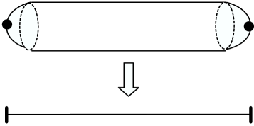
Figure 1: 6d theory on a sphere with two full punctures, and its reduction to 5d theory. The punctures become boundary conditions.

Next, let us consider 6d theory of type $A_{N-1}$ on a sphere of area $\mathcal{A}$, with two full punctures, each carrying $\mathrm{SU}(N)$ global symmetry. We choose the metric on the sphere so that it looks like a cylinder of circumference $R_{6}$ and length $R_{5}$ with $R_{6}\ll R_{5}$, capped by disks each with a full puncture at the center, see Fig. 1.

This system can be analyzed as the 5d maximally-supersymmetric $\mathrm{SU}(N)$ Yang-Mills with coupling constant $1/g^{2}_{5d}\sim 1/R_{6}$, put on a segment with length $R_{5}$, with Dirichlet boundary condition at both ends. The BPS equation whose solution corresponds to a point in the Higgs branch is the Nahm equation on the segment $s\in[0,R_{5}]$:

$$\frac{d}{ds}\Phi_{i}+[A_{s},\Phi_{i}]=\epsilon_{ijk}[\Phi_{j},\Phi_{k}]$$ (2.3)

where $i,j,k$ run from $1$ to $3$. The Dirichlet boundary conditions of the Yang-Mills theory imply that $\Phi_{i}(s)$ should be regular at both boundaries. We identify two solutions related by a gauge transformation $h:[0,R_{5}]\to\mathrm{SU}(N)$ such that $h(0)=h(R_{5})=1$. The metric on the moduli space comes from the kinetic terms in the 5d Lagrangian, and, analogously to the case in the previous subsection, it has a factor of $1/\mathcal{A}\sim 1/(R_{5}R_{6})$ in it. We will denote this hyperkähler moduli space by $I(\mathcal{A})$. Since the group of all maps $h:[0,R_{5}]\to\mathrm{SU}(N)$ acts on solutions to (2.3) there is a global $\mathrm{SU}(N)\times\mathrm{SU}(N)$ symmetry acting on $I(\mathcal{A})$, where the two factors are obtained from $h(0)$ and $h(R_{5})$.

The moduli space $I(\mathcal{A})$ can be parametrized by $g=P\exp\int_{0}^{R_{5}}A_{s}ds$ and $\Phi_{i}(0)$. Therefore it is topologically $\simeq\mathrm{SU}(N)\times\mathfrak{su}(N)^{3}$. Let us consider a point $(g,\phi_{i})$ in it. Then the global symmetry element $(h_{1},h_{2})\in\mathrm{SU}(N)_{1}\times\mathrm{SU}(N)_{2}$ acts via

$$(g,\phi_{i})\to(h_{1}gh_{2}^{-1},h_{1}\phi_{i}h_{1}^{-1}).$$ (2.4)

Of course, at a general point on the moduli space the global symmetry is broken to a discrete group (the center of $\mathrm{SU}(N)$, diagonally embedded). However, even when $\phi_{i}=0$, the global symmetry $\mathrm{SU}(N)_{1}\times\mathrm{SU}(N)_{2}$ is spontaneously broken to a diagonal subgroup $\mathrm{SU}(N)$ specified by $h_{1}=gh_{2}g^{-1}$. In particular, there is no point where the whole of the global symmetry $\mathrm{SU}(N)^{2}$ is unbroken. The largest isotropy group of any point is $\mathrm{SU}(N)$.

Now let us consider taking the limit $\mathcal{A}\to 0$. Once again, as discussed in the Introduction, one must choose a point around which to expand. It is instructive to see how the global symmetries behave in this limit. The most symmetric point we can choose is $(1,\vec{0})\in\mathrm{SU}(N)\times\mathfrak{su}(N)^{3}$. As before, the limiting metric is just the flat metric on the tangent space at $(1,\vec{0})$, which is isomorphic to $\mathfrak{su}(N)\oplus\mathfrak{su}(N)^{3}\cong\mathfrak{su}(N)\otimes\mathbb{H}$. The $\mathrm{SU}(N)\times\mathrm{SU}(N)$ symmetry was broken to the diagonal $\mathrm{SU}(N)$. The broken anti-diagonal symmetries contract to translations by $\mathbb{R}^{N^{2}-1}$. The isometry group of the IR limit, commuting with the hyperkähler structure, is just the semidirect product of translations with $\mathrm{Sp}(N^{2}-1)$.

This example illustrates two points: i) some of the global symmetry at nonzero $\mathcal{A}$ can get contracted in the limit, and ii) the global symmetry after $\mathcal{A}\to 0$ limit can be enhanced.

3 Higgs branch for $C$ with finite area

Having seen two easy examples, let us discuss the general case of $A_{N-1}$ theories of class $S$ described in the Introduction. As we mentioned there, each defect is labeled by a map $\rho:\mathrm{SU}(2)\to\mathrm{SU}(N)$. (These defects admit mass deformations. However in this paper we take the mass deformations to be zero.) Equivalently, $\rho$ is given by a partition $(\lambda_{1},\lambda_{2},\ldots)$ of $N$. We use the notation so that, for example, $\rho=[3^{2}1^{2}]$ stands for the partition $8=3+3+1+1$. The puncture of type $\rho$ has a flavor symmetry $G^{\rho}$, which is the commutant of the image of $\rho$ inside $G$. The punctures corresponding to $f=[1^{N}]$ and $s=[N-1,1]$ are particularly important and are called full and simple, respectively; the puncture $\rho=[N]$ corresponds to the absence of the puncture altogether. The full puncture has $\mathrm{SU}(N)$ flavor symmetry, and the simple puncture has $\mathrm{U}(1)$ flavor symmetry. We first analyze the Higgs branch of this system in two ways in Sections 3.1 and 3.2, then we apply those two viewpoints.

3.1 As the Coulomb branch of 5d super Yang-Mills on $C$

Let us consider our 4d system on $S^{1}$, of circumference $R$. It has 3d $\mathcal{N}=4$ symmetry. The Higgs branch does not depend on $R$; but as the metric of the moduli space has mass dimension two and one in spacetime dimension four and three, respectively, it is natural to set

$$ds^{2}(\text{4d Higgs branch})=R^{-1}ds^{2}(\text{3d Higgs branch}).$$ (3.1)

We now have 6d theory compactified on $S^{1}\times C$. We can perform the compactification on $S^{1}$ first, and regard the system as 5d maximally-supersymmetric $\mathrm{SU}(N)$ Yang-Mills on $C$ with codimension-two defects $D(\rho_{i})$. The coupling constant is as always $1/g^{2}_{5d}\sim 1/R$. Since 5d SYM is IR free we can identify the defects as 3d superconformal field theories coupled to the bulk. It turns out these are just the theories called $T_{\rho}[\mathrm{SU}(N)]$ in [6]. This procedure is effectively the 3d mirror operation, and as such the original Higgs branch is the Coulomb branch of this 3d system obtained by compactifying the 5d SYM on $C$.

As a 3d theory, our 5d SYM on $C$ has an infinite-dimensional gauge group of maps from $C$ to $\mathrm{SU}(N)$. The 5d kinetic term

$$\int_{\mathbb{R}^{3}}d^{3}x\int_{C}dzd\bar{z}e^{\phi}\frac{1}{g^{2}_{5d}}\mathrm{tr}F_{\mu\nu}F_{\mu\nu}$$ (3.2)

can be thought of defining a coupling matrix on the gauge algebra of maps $X,Y:C\to\mathfrak{su}(N)$ via

$$\int_{C}dzd\bar{z}e^{\phi}\frac{1}{g^{2}_{5d}}\mathrm{tr}XY.$$ (3.3)

Here we used the complex structure and the Weyl mode to express the 2d metric on $C$. This infinite-dimensional group is always broken down to $\mathrm{SU}(N)$, which corresponds to constant maps from $C$ to $\mathrm{SU}(N)$. Effectively, our 3d theory is just $\mathrm{SU}(N)$ $\mathcal{N}=4$ theory coupled to $g$ hypermultiplets in the adjoint representation of $\mathrm{SU}(N)$ and $T_{\rho_{i}}[\mathrm{SU}(N)]$ where $i=1,\ldots,n$ and $g$ is the genus of $C$. The adjoint hypermultiplets come from the zero modes of $A_{z}$, $A_{\bar{z}}$ on $C$.

The metric of the Coulomb branch only depends on the coupling constant of the unbroken gauge group, and not on the coupling matrix of the broken part of the gauge fields. The coupling constant of the unbroken $\mathrm{SU}(N)$ gauge field is given by

$$\frac{1}{g_{3}^{2}}=\frac{\int_{C}dzd\bar{z}e^{\phi}}{g_{5}^{2}}=\frac{\mathcal{A}}{R}.$$ (3.4)

As this is the only scale in the system, the metric on the 3d Coulomb branch has an overall factor of $R/\mathcal{A}$. Combining with (3.1), we see that the 4d Higgs branch has an overall factor of $1/\mathcal{A}$. Let us stress that the metric does not depend on the detailed form of the Weyl mode $e^{\phi}$.

Recall that $T_{\rho}[\mathrm{SU}(N)]$ has a linear quiver realization [6]: for a partition $\rho=[\lambda_{1},\lambda_{2},\ldots,\lambda_{k}]$ with $\lambda_{1}\geq\lambda_{2}\geq\cdots$, the quiver is

$$\underline{\mathrm{SU}(N)}-\mathrm{U}(n_{1})-\mathrm{U}(n_{2})-\cdots-\mathrm{U}(n_{k-1})$$ (3.5)

where $n_{s}=\sum_{s<t}\lambda_{t}$; the underlined group is a flavor symmetry. $T_{\rho}[\mathrm{SU}(N)]$ is defined to be the limit where the gauge coupling of all the gauge groups are taken to infinity.

Then our Coulomb branch is obtained by taking the linear quiver realizations of $T_{\rho_{i}}[\mathrm{SU}(N)]$ for each $\rho_{i}$, and coupling it to an $\mathrm{SU}(N)$ and $g$ adjoint hypermultiplets [11]. We keep the gauge coupling of the central $\mathrm{SU}(N)$ finite, given by (3.4), but take the coupling constants of all the other gauge groups to be infinitely large.

Let us consider the genus zero case, and consider defects labeled by partitions $\rho_{i}=[\lambda_{i,1},\lambda_{i,2},\ldots]$. Then the central $\mathrm{SU}(N)$ has in total

$$N_{f}=\sum_{i}n_{i,1}=\sum_{i}(N-\lambda_{i,1})$$ (3.6)

fundamental flavors. Depending on whether $N_{f}\geq 2N$, $N_{f}=2N-1$, or $N_{f}\leq 2N-2$, the dynamics of the $\mathrm{SU}(N)$ gauge multiplet is “good”, “ugly” or “bad” in the terminology of [6]. In our context, when it is good the $\mathcal{A}\to 0$ limit gives us an interacting 4d theory; when it is ugly the $\mathcal{A}\to 0$ limit gives us a free 4d theory, or an interacting theory with a free subsector; when it is bad, more data is needed to specify an $\mathcal{A}\to 0$ limit. In contrast to the example in Sec. 2.2 there is no canonical place in the moduli space to take the limit. In the “bad” cases the $R$-symmetries and global symmetries in the UV and IR theories can be quite different. When $g>1$, the theory is always good. When $g=1$, the theory is bad when there is no puncture, ugly when there is only one simple puncture, and good otherwise.

Let us conclude with several remarks:

1. This approach to the moduli space tells us when the limit $\mathcal{A}\to 0$ is easily taken. But it does not give us a way to calculate the metric, because we do not quite know how to determine the exact, quantum-corrected metric on the Coulomb branch of a 3d $\mathcal{N}=4$ gauge theory yet. However, this expression has the virtue of showing its independence from the nonzero modes of the Weyl factor of the metric on $C$. In the following, we denote the Higgs branch by $\eta(C,D,\mathcal{A})$, where $D=\{D(\rho_{i})\}$. We also denote it as $\eta(C_{\rho_{1},\ldots,\rho_{n}},\mathcal{A})$.

2. It is worth remarking that the good/ugly/bad trichotomy can also be detected by studying the virtual dimension of the mass-dimension $N$ part of the Coulomb branch of the would-be 4-dimensional field theory of the $\mathcal{A}\to 0$ limit, when $g=0$. Each defect is characterized by $\rho_{i}$. By Riemann-Roch, the virtual dimension of the mass-dimension $N$ part of the Coulomb branch of $S_{N}[C,D]$ is

   $$\dim_{\mathbb{C}}{\cal M}^{\text{Coulomb}}_{\text{mass dim}=N}=-(2N-1)+\sum_{i}(N-\lambda_{i,1})$$ (3.7)

   Then the good/ugly/bad trichotomy corresponds to the cases where $\dim_{\mathbb{C}}{\cal M}^{\text{Coulomb}}_{\text{mass dim}=N}$ is positive, zero, and negative, respectively.

3. In [6] the good/bad/ugly trichotomy was established by studying the conformal dimensions of monopole operators. In the good cases the monopole operators have positive dimension, as computed from the R-symmetry. In the the ugly cases, they are free fields. In the bad cases they have dimensions violating the unitarity bound as computed from the naive R-symmetry. In the bad cases one thus concludes that the IR R-symmetry must be different from the UV R-symmetry. These monopole operators come from monopole strings in the 5d SYM theory wrapped on $C$. These in turn come from the surface defects of the 6d theory wrapped on $C$. Their holographic duals are then given by M2-branes wrapped on $C$. In this last setting the associated chiral operators of the 4d theory were considered in [12]. This is useful since, in principle, one could compute the conformal dimensions of these operators via the AdS/CFT correspondence.

4. Although we are focused here on the $\mathcal{A}\to 0$ limit, it is worth noting that the $\mathcal{A}\to\infty$ limit is a weak coupling limit, and in this limit the metric on the moduli space approaches a product metric on a fibration over $(\mathbb{R}^{3}\times S^{1})^{N-1}/\mathfrak{S}_{N}$ whose fiber is $\prod_{i}\mathcal{M}^{\rm Coul}(T_{\rho_{i}})$. Recall from [6] that $\mathcal{M}^{\rm Coul}(T_{\rho_{i}})=S_{\rho_{i}}\cap\mathcal{N}$ is the intersection of a Slodowy slice with the nilpotent cone. Thus, in the $\mathcal{A}\to\infty$ limit the Higgs moduli space can be made rather explicit.

3.2 As a hyperkähler quotient

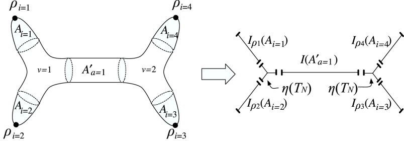
Figure 2: Left: a skeleton-like metric on $C$. Right: its reduction to 5d. The Higgs branch of the each component is named. The Higgs branch of the total system is given by the hyperkähler quotient via the diagonal $\mathrm{SU}(N)$ actions.

As a second method, consider putting on $C$ a metric of cylinders of circumference $R_{6}$ joined at three-pronged junctures, so that the punctures are at the center of the caps, see Fig. 2. The Higgs branch is then that of 5d maximally-supersymmetric Yang-Mills with coupling constant $1/g^{2}_{5d}\sim 1/R_{6}$ on a trivalent graph. The original codimension-two defect at $p$ labeled by $\rho:\mathrm{SU}(2)\to\mathrm{SU}(N)$ becomes a supersymmetric boundary of the 5d Yang-Mills, given by

$$\Phi_{i}(s)\sim\rho(t^{i})/s+\Phi^{0}_{i}+{\cal O}(s)$$ (3.8)

where $t^{j}=\frac{i}{4}\sigma^{j}$ is a basis of generators of $\mathfrak{sl}(2,\mathbb{C})$, $s$ is the distance to the boundary, and $\Phi^{0}_{i}$ must be in the commutant of $\rho$. The junction of three segments is a supersymmetric boundary condition of $\mathrm{SU}(N)^{3}$ super Yang-Mills; we have the 4d $T_{N}$ theory with $\mathrm{SU}(N)^{3}$ living on the boundary. Therefore, the Higgs branch of this system is given by the hyperkäher quotient

$$\eta(C,D,\mathcal{A})=\left[\prod_{i}I_{\rho_{i}}(\mathcal{A}_{i})_{i}\times\prod_{a}I(\mathcal{A}_{a}^{\prime})_{a,1;a,2}\times\prod_{v}\eta(T_{N})_{v,1;v,2;v,3}\right]/\!/\!/\prod_{j=1}^{3n_{v}}\mathrm{SU}(N).$$ (3.9)

Here, $I_{\rho}(\mathcal{A})$ is the moduli space of the Nahm equation on a segment of length $\mathcal{A}$ with a boundary condition (3.8) on one side and with $\Phi_{i}(s)$ regular on the other side. $I(\mathcal{A})$ is an abbreviation for $I_{\rho}(\mathcal{A})$ where $\rho$ is zero. Moreover $\eta(T_{N})$ is the Higgs branch of the 4d $T_{N}$ theory. The labels $i$, $a$ and $v$ enumerate the external edges, the internal edges and the trivalent vertices respectively. $\mathcal{A}_{i}$ and $\mathcal{A}_{a}^{\prime}$ are the areas of the external and internal cylinders, respectively. The trinions carry zero area.

Here and in the following, we have actions of many copies of $\mathrm{SU}(N)$ on the spaces. To distinguish them, we put subscripts to the spaces as in (3.9), so that $\mathrm{SU}(N)_{i}$ act on $I_{\rho_{i}}(\mathcal{A}_{i})_{i}$, $\mathrm{SU}(N)_{a,1}\times\mathrm{SU}(N)_{a,2}$ on $I(\mathcal{A}^{\prime}_{a})_{a,1;a,2}$, and $\mathrm{SU}(N)_{v,1}\times\mathrm{SU}(N)_{v,2}\times\mathrm{SU}(N)_{v,3}$ on $\eta(T_{N})_{v,1;v,2;v,3}$. The numerator of (3.9) has an action by $6n_{v}$ copies of $SU(N)$. A subgroup, defined by the diagonal combinations of $\mathrm{SU}(N)\times\mathrm{SU}(N)$ which are glued together, and isomorphic to $3n_{v}$ copies of $SU(N)$, is gauged. In the following, we denote by $\mathrm{SU}(N)_{a,b}$ the diagonal subgroup of $\mathrm{SU}(N)_{a}\times\mathrm{SU}(N)_{b}$.

This construction is closely related to and partially overlaps with the bow construction of Cherkis and collaborators [13, 14, 15, 16, 17, 18]. Our $I_{\rho}(\mathcal{A})$ is their bow. Instead of their arrows, we have trivalent vertices.

$I_{\rho}(\mathcal{A})$ is a relatively well-studied manifold which we will review below; the structure of $\eta(T_{N})$ is also partially known. Therefore this expression gives us a practical way to study the Higgs branch. Note that this equality asserts that the hyperkähler quotient on the right hand side only depends on $\mathcal{A}_{i},\mathcal{A}_{a}^{\prime}$ through the sum $\mathcal{A}=\sum\mathcal{A}_{i}+\sum\mathcal{A}_{a}^{\prime}$. We will explain why this is so in Sec. 3.5. First, we need to recall some basic properties of $I_{\rho}(\mathcal{A})$ and $\eta(T_{N})$.

3.3 The manifold $I_{\rho}(\mathcal{A})$

An important special case of the above construction is the case where $C$ is a Riemann sphere with two punctures, where one puncture is characterized by $\rho$ and another puncture is full, $f=[1^{N}]$. This gives the Higgs branch moduli space $I_{\rho}(\mathcal{A})$. In the general notation this is $\eta(C,\{D(\rho),D(f)\},\mathcal{A})=\eta(C_{\rho,f},\mathcal{A})$.

We review here the structure of the manifold $I_{\rho}(\mathcal{A})$, which is the moduli space of the Nahm’s equation where $\Phi_{i}(s)$ satisfy the boundary condition (3.8) on one end, and are regular at the other end. This moduli space was studied mathematically [19, 20, 21] and was given physical interpretation in Sec. 3.9 of [22]. We only quote salient results here; the details can be found op. cit.

We already saw $I(\mathcal{A})$ in Sec. 2.2. As a holomorphic symplectic manifold, this is $T^{*}\mathrm{SU}(N)_{\mathbb{C}}$, which is further isomorphic to $\mathrm{SU}(N)_{\mathbb{C}}\times\mathfrak{su}(N)_{\mathbb{C}}$ using the left-invariant one-forms. The space $I_{\rho}(\mathcal{A})$ is, as a complex manifold, a subspace of $I(\mathcal{A})$ given by

$$\mathrm{SU}(N)_{\mathbb{C}}\times S_{\rho}\subset\mathrm{SU}(N)_{\mathbb{C}}\times\mathfrak{su}(N)$$ (3.10)

where $S_{\rho}$ is the Slodowy slice at $\rho(t^{+})$, defined by

$$S_{\rho}=\{\rho(t^{+})+x\bigm{|}[\rho(t^{-}),x]=0\}.$$ (3.11)

Here $t^{\pm}$ are raising/lowering operators in $\mathfrak{sl}(2)$. Note that the dimension of $S_{\rho}$ is the number of irreducible components of $\mathfrak{su}(N)$ regarded as an $\mathrm{SU}(2)$ representation under the homomorphism $\rho$. The complex moment map of the $\mathrm{SU}(N)$ action on $I_{\rho}(\mathcal{A})$ at $(g,X)\in\mathrm{SU}(N)_{\mathbb{C}}\times S_{\rho}$ is $gXg^{-1}$.

From the description as the moduli space of the Nahm equation, it is clear that

$$I_{\rho}(\mathcal{A}+\mathcal{A}^{\prime})=I_{\rho}(\mathcal{A})\times I(\mathcal{A}^{\prime})/\!/\!/\mathrm{SU}(N).$$ (3.12)

As a side remark we note that, more generally, for the sphere with two  punctures $D(\rho_{1})$ and $D(\rho_{2})$ the moduli space $\eta(C,\{D(\rho_{1}),D(\rho_{2})\},\mathcal{A})$ is the moduli space of solutions to Nahm’s equations on the interval $[0,\mathcal{A}]$ with Nahm-type boundary conditions of type $\rho_{1},\rho_{2}$ at the two ends. As a holomorphic manifold this is just

$$\{(g,X)|X\in S_{\rho_{1}}\cap g^{-1}S_{\rho_{2}}g\}\subset T^{*}\mathrm{SU}(N)_{\mathbb{C}}.$$ (3.13)

A sphere with fewer punctures can be obtained by setting one or two of $\rho_{1,2}$ to be $[N]$, because a puncture with $\rho=[N]$ is equivalent to having no puncture. In particular, the sphere with no punctures at all corresponds to the manifold

$$\{(g,X)|X\in S_{[N]}\cap g^{-1}S_{[N]}g\}\subset T^{*}\mathrm{SU}(N)_{\mathbb{C}},$$ (3.14)

and in fact is the moduli space of centered BPS monopoles with $\mathrm{SU}(2)$ gauge group and magnetic charge $N$.

3.4 The sphere with three full punctures and the manifold $\eta(T_{N})$

We now consider the case where $C$ is a sphere with three full punctures. The 4d $\mathcal{A}\to 0$ limit leads to the trinion theories $T_{N}$ introduced in [3]. We denote its Higgs branch by $\eta(T_{N})$. In our general notation this is $\eta(C,\{D(f),D(f),D(f)\},0)=\eta(C_{fff},0)$.

The space $\eta(T_{N})$ is known to have the following properties [12, 23, 11, 7]. It is a hyperkähler cone whose complex dimension is

$$\dim_{\mathbb{C}}\eta(T_{N})=3(N^{2}-1)-(N-1),$$ (3.15)

with a triholomorphic action of $\mathrm{SU}(N)^{3}$. It is also the Coulomb branch of the star-shaped 3d quiver gauge theory in the limit where all gauge coupling constants are taken to be infinite, or equivalently the Coulomb branch of the 3d $\mathrm{SU}(N)$ theory coupled to three copies of $T[\mathrm{SU}(N)]$ theory in the infinite coupling limit, as we recalled in Sec. 3.1. We stress that for $\eta(T_{N})$ we have already taken the $\mathcal{A}\to 0$ limit, so that it does not contribute to the overall area in equation (3.9).

$\eta(T_{2})$ is a flat hyperkähler manifold $\mathbb{H}^{4}$ with $\mathrm{SU}(2)^{3}$ action, $\eta(T_{3})$ is the minimal nilpotent orbit of $(E_{6})_{\mathbb{C}}$. $\eta(T_{N})$ with $N>3$ is not explicitly known, but the following two important properties have been inferred from various dualities.

First, S-duality of two copies of the 4d $T_{N}$ theory coupled to $\mathrm{SU}(N)$, as described in [3], implies the equality of the hyperkähler manifold with action of $\mathrm{SU}(N)_{1}\times\mathrm{SU}(N)_{2}\times\mathrm{SU}(N)_{3}\times\mathrm{SU}(N)_{4}$:

$$\eta(T_{N})_{1,2,a}\times\eta(T_{N})_{3,4,b}/\!/\!/\mathrm{SU}(N)_{a,b}=\eta(T_{N})_{1,3,a}\times\eta(T_{N})_{2,4,b}/\!/\!/\mathrm{SU}(N)_{a,b}$$ (3.16)

where $\eta(T_{N})_{1,2,3}$ stands for $\eta(T_{N})$ where $\mathrm{SU}(N)_{1}\times\mathrm{SU}(N)_{2}\times\mathrm{SU}(N)_{3}$ acts on it; the quotient is taken with respect to the diagonal subgroup of $\mathrm{SU}(N)_{a}\times\mathrm{SU}(N)_{b}$, which we denoted by $\mathrm{SU}(N)_{a,b}$.

A second important piece of information is about the moment maps. Let us denote the complex moment maps for $\mathrm{SU}(N)_{i}$ ($i=1,2,3$) as $(\mu_{i})_{\mathbb{C}}:\eta(T_{N})\to\mathfrak{su}(N)_{\mathbb{C}}$. Then it is believed that $\mathrm{tr}(\mu_{i})_{\mathbb{C}}^{k}$ is independent of $i$. (See [11] for the argument.) In particular,

$$\mathrm{tr}(\mu_{1})_{\mathbb{C}}^{2}=\mathrm{tr}(\mu_{2})_{\mathbb{C}}^{2}=\mathrm{tr}(\mu_{3})_{\mathbb{C}}^{2}.$$ (3.17)

3.5 Dependence on area from the perspective of the quotient

Readers interested mainly in the 4d theories can skip this and the next subsections and can directly go to Sec. 4. Given (3.12) and (3.16), the proof that the right hand side of (3.9) only depends on $\mathcal{A}=\sum\mathcal{A}_{i}+\sum\mathcal{A}_{i}^{\prime}$ and is furthermore independent of the pants decomposition boils down to the property

$$I(\mathcal{A})_{1,a}\times\eta(T_{N})_{b,2,3}/\!/\!/\mathrm{SU}(N)_{a,b}=\eta(T_{N})_{1,2,a}\times I(\mathcal{A})_{b,3}/\!/\!/\mathrm{SU}(N)_{a,b},$$ (3.18)

see Fig. 3.

Figure 3: The property (3.18) illustrated. The action of $\mathrm{SU}(N)_{i}$ is labeled by $i$ in the figure.

To show this, let us consider a more general procedure, which we can call the hyperkähler modification. Let $Y$ be a hyperkähler manifold with a triholomorphic action of $G$, whose moment map is (after a choice of complex structure) $(\mu_{\mathbb{C}},\mu_{\mathbb{R}})$. We define the modification $Y(\mathcal{A})$ to be

$$Y(\mathcal{A})_{1}=I(\mathcal{A})_{1,a}\times Y_{b}/\!/\!/G_{a,b}.$$ (3.19)

As a holomorphic symplectic manifold, $Y(\mathcal{A})$ is the same as the original $Y$: first, note that

$$T^{*}G_{\mathbb{C}}\times Y/\!/\!/G=\{(g,X,y)\in G_{\mathbb{C}}\times{\displaystyle\mathfrak{g}}_{\mathbb{C}}\times Y\,|\,X+\mu_{\mathbb{C}}(y)=0\}/\sim$$ (3.20)

where $(g,X,y)\sim(gh,hXh^{-1},h\cdot y)$, where $h\cdot y$ stands for the action of $h\in G$ on $y\in Y$. Then $X$ is determined by $\mu_{\mathbb{C}}(y)$ and $g$ can be gauge fixed to be the identity. Therefore, as a complex manifold, $Y(\mathcal{A})$ is canonically identified with $Y$. One can also check that the holomorphic symplectic form does not change.

The hyperkähler metric, however, changes. The way it changes can be found by studying the twistor space, at least in the case that $Y$ has an $SO(3)$ group of isometries which rotate the three complex structures. In particular, this applies when $Y$ is a Higgs branch of a four-dimensional $\mathcal{N}=2$ theory, and also to the Higgs branch at finite $\mathcal{A}$. Recall that Hitchin’s theorem states that, roughly speaking, the twistor family of holomorphic symplectic manifolds is equivalent to the hyperkähler metric.

The twistor space of $I(\mathcal{A})$ was found by Kronheimer [19]: the transition function at the equator is given by

$$(g,X,\zeta)\to(g\exp(2\mathcal{A}X/\zeta),X\zeta^{-2},\zeta^{\prime})$$ (3.21)

where $(g,X)\in G_{\mathbb{C}}\times{\displaystyle\mathfrak{g}}_{\mathbb{C}}$ and $\zeta^{\prime}=1/\zeta$. Using the $SO(3)$ isometry rotating the three complex structures, the twistor space of $Y$ can be holomorphically trivialized on the northern and southern hemispheres of the twistor sphere and hence the twistor space of $Y$ can be presented as

$$(y,\zeta)\to(\phi_{\zeta}(y),\zeta^{\prime}).$$ (3.22)

Now, because the $G$-action is triholomorphic the moment map satisfies

$$\zeta^{-2}\mu_{\mathbb{C},\zeta}(y)=\mu_{\mathbb{C},\zeta^{\prime}}(\phi_{\zeta}(y))$$ (3.23)

and hence the equation $X+\mu_{\mathbb{C},\zeta}(y)=0$ is consistent across patches. After choosing the gauge $g=1$ and eliminating $X$ we find that the twistor space of $Y(\mathcal{A})$ is given by

$$(y,\zeta)\to(\exp\left(-2\mathcal{A}\mu_{\mathbb{C},\zeta}(y)/\zeta\right)\phi_{\zeta}(y),\zeta^{\prime}).$$ (3.24)

Infinitesimally, the action of $\exp(2\mathcal{A}\mu_{\mathbb{C},\zeta}(y)/\zeta)$ on $Y$ is generated by the vector field $v=2\sum_{a}\mu_{\mathbb{C},\zeta}^{a}v^{a}/\zeta$ where $a$ is the adjoint index and $v^{a}$ is the vector field for the $a$-th generator of $G$. It is easy to see that $v$ is in fact the Hamiltonian vector field for $\mathrm{tr}\mu_{\mathbb{C},\zeta}^{2}/\zeta$. Therefore, the deformation $Y(\mathcal{A})$ of $Y$ is determined once the quadratic Casimir of the complex moment map, $\mathrm{tr}\mu_{\mathbb{C},\zeta}^{2}$ is given for every complex structure $\zeta$. Applying this constructing to $\eta(T_{N})$ and invoking the property (3.17) we establish (3.18), the desired identity.

In fact, we can say a little more about how the metric is deformed by $\mathcal{A}$. Using the results of [27] (see their eq. (4.27)), we can extract the modification of the Kähler potential from the modification (3.24) in the twistor construction. Denoting $K(\mathcal{A})$ be the Kähler potential of $Y(\mathcal{A})$ in the complex structure $I$, we have

$$\frac{d}{d\mathcal{A}}K(\mathcal{A})=\mathrm{Re}\ \mathrm{tr}\ \mu_{\mathbb{C}}^{2}$$ (3.25)

where $\mu_{\mathbb{C}}$ is the complex moment map in the complex structure $J$.

3.6 A connection with the bow construction

Before proceeding, let us consider $\eta(C,\{D(f),D(f),D(s)\},\mathcal{A})$ for a three-punctured sphere $C$. At $\mathcal{A}=0$, this is just the bifundamental hypermultiplet Higgs branch $B_{1,2}=\mathbb{C}^{N^{2}}\oplus\mathbb{C}^{N^{2}}$ with a natural $\mathrm{SU}(N)_{1}\times\mathrm{SU}(N)_{2}$ action. Then at nonzero $\mathcal{A}$, it is given by

$$I(\mathcal{A}^{\prime})_{1,a}\times B_{b,c}\times I(\mathcal{A}^{\prime\prime})_{d,2}/\!/\!/\mathrm{SU}(N)_{a,b}\times\mathrm{SU}(N)_{c,d}$$ (3.26)

where $\mathcal{A}=\mathcal{A}^{\prime}+\mathcal{A}^{\prime\prime}$. That this quotient only depends on the sum $\mathcal{A}^{\prime}+\mathcal{A}^{\prime\prime}$ follows from the fact that $\mathrm{tr}\mu_{\mathbb{C}}^{(1)}{}^{2}=\mathrm{tr}(AB)^{2}$ and $\mathrm{tr}\mu_{\mathbb{C}}^{(2)}{}^{2}=\mathrm{tr}(BA)^{2}$ are equal. The dependence only on the sum is also known in the context of the bow construction. As shown in [17], this is a stratum in the moduli space of $\mathrm{SU}(2N)$ BPS monopoles on $\mathbb{R}^{3}$ with one Dirac singularity where the vev of the adjoint scalar is given by $\mathop{\mathrm{diag}}(\underbrace{a,\ldots,a}_{N},\underbrace{-a,\ldots,-a}_{N})$. The difference $\mathcal{A}^{\prime}-\mathcal{A}^{\prime\prime}$ gives the B-field on $\mathbb{R}^{3}$ but it does not affect the moduli metric.

4 Application to the 4d analysis

We now return to the subtleties in the factorization statement (1.2). When $C$ factorizes we expect the Higgs branches of the theories to be related by hyperkähler gluing. In particular, if we factorize on full punctures then the diagonal of the global $\mathrm{SU}(N)\times\mathrm{SU}(N)$ symmetry of the $C_{L}\sqcup C_{R}$ theory is gauged. Thus, the moment maps $\mu_{L}$ and $\mu_{R}$ of the flavor symmetries at $p_{L},p_{R}$ are identified: $\mu_{L}+\mu_{R}=0$. Now suppose that the six-dimensional theory associated to $C_{R}$ is bad. Then, no point on the Higgs branch has $\mu_{R}=0$. Then the $\mathrm{SU}(N)$ symmetry is always spontaneously broken, and the $\mathcal{A}\to 0$ limit forces $\mu_{R}$, and hence $\mu_{L}$ to go to infinity. The vacuum flows to that of a new theory, and in the limit the gauge symmetry can become smaller. In the “ugly” theories, there is a point where $\mu_{R}=0$. We now examine some special cases of such bad and ugly theories by studying some trinion theories $C$ with defects $D(\rho_{1}),D(\rho_{2}),D(\rho_{3})$. We denote them by $C_{\rho_{1},\rho_{2},\rho_{3}}$.

4.1 $T_{N}$ and the bifundamental

First, let us compare a sphere $C_{fff}$ with three full punctures and a sphere $C_{ffs}$ with two full punctures and one simple puncture. Recall that the full puncture is $f=[1^{N}]$ and the simple puncture is $s=[N-1,1]$. At finite non-zero area, the Higgs branch of $C_{ffs}$ is given by

$$\eta(C_{ffs},\mathcal{A})_{1,2}=I_{s}(\mathcal{A})_{a}\times\eta(T_{N})_{b,1,2}/\!/\!/\mathrm{SU}(N)_{a,b}.$$ (4.1)

As a complex manifold, $I_{s}(\mathcal{A})\simeq\mathrm{SU}(N)_{\mathbb{C}}\times S_{s}$ as discussed before. As $\dim_{\mathbb{C}}S_{s}=N+1$, $\dim_{\mathbb{C}}I_{s}(\mathcal{A})=N^{2}+N$. The $\mathrm{SU}(N)$ action on $I_{s}(\mathcal{A})$ is free. Therefore the dimension of $\eta(C_{ffs},\mathcal{A})$ is

$$\dim_{\mathbb{C}}\eta(C_{ffs},\mathcal{A})=\dim_{\mathbb{C}}\eta(T_{N})+\dim_{\mathbb{C}}I_{s}(\mathcal{A})-2\dim\mathrm{SU}(N)=2N^{2}.$$ (4.2)

If we use the mirror quiver as in Sec. 3.1, the central node has $N_{f}=2N-1$, and is “ugly,” in the terminology of [6]. Therefore we expect to have $N^{2}$ free hypermultiplets in the $\mathcal{A}\to 0$ limit. This matches our expectation that the 6d theory on $C_{ffs}$ at zero area gives the bifundamental hypermultiplet of $\mathrm{SU}(N)^{2}$. For $N=3$, the equation of $\eta(T_{3})$ is known [28], and the quotient (4.1) can in principle be explicitly performed at the level of the holomorphic symplectic quotient.

4.2 The trinion with one full and two simple punctures

Next, let us consider a sphere $C_{fss}$ with one full puncture and two simple punctures. At finite nonzero area, the Higgs branch is given by

$$\eta(C_{fss},\mathcal{A})_{1}=I_{s}(\mathcal{A})_{a}\times\eta(C_{ffs},0)_{b,1}/\!/\!/\mathrm{SU}(N)_{a,b}$$ (4.3)

where $\eta(C_{ffs},0)$ is the linear space of a bifundamental. The dimension is easily calculated:

$$\dim_{\mathbb{C}}\eta(C_{fss},\mathcal{A})=\dim_{\mathbb{C}}\eta(C_{ffs},0)+\dim_{\mathbb{C}}I_{s}(\mathcal{A})-2\dim\mathrm{SU}(N)=N^{2}+N+2.$$ (4.4)

This space has a triholomorphic action of $\mathrm{SU}(N)$, but there is no point on this space where it is unbroken: if it were unbroken then the dimension would need to be at least $2(N^{2}-1)$. But $2(N^{2}-1)$ is larger than (4.4) for $N>2$.

We believe that there is another equivalence of the hyperkähler spaces

$$\eta(C_{fss},\mathcal{A})_{1}=I_{t}(\mathcal{A})_{1}\times(\mathbb{C}^{2}\oplus\mathbb{C}^{2})/\!/\!/\mathrm{SU}(2)$$ (4.5)

where $t$ is the partition $[N-2,1,1]$, and the $\mathrm{SU}(2)$ action is the diagonal action between the commutant of $t(\mathrm{SU}(2))$ inside $\mathrm{SU}(N)$ and a natural action of $\mathrm{SU}(2)$ on $\mathbb{C}^{2}\oplus\mathbb{C}^{2}$. This equality can in principle be proven by expressing the right hand sides of (4.3) and (4.5) as the moduli spaces of the Nahm equation. This relation can also be inferred from the analysis of the S-dual of $\mathrm{SU}(N)$ with $2N$ flavors [8].

Now we can have a new insight why we had $\mathrm{SU}(2)$ as the gauge symmetry in the strong-coupling limit of $\mathrm{SU}(N)$ theory with $2N$ flavors. As in [3] we start from a sphere with two full punctures and two simple punctures, $C_{ffss}$. When two simple punctures are close, at finite nonzero area $\mathcal{A}$, we have a sphere $C_{fff}$ coupled to a sphere $C_{fss}$ with area $\mathcal{A}$. Now the latter is equivalent to a two-punctured sphere $C_{ft}$ with area $\mathcal{A}$ coupled to a doublet $\mathbb{C}^{2}\oplus\mathbb{C}^{2}$ of $\mathrm{SU}(2)$. So, we have $C_{fft}$ with area $\mathcal{A}$ coupled to a doublet of $\mathrm{SU}(2)$ by a gauge group $\mathrm{SU}(2)$, see Fig. 4. At this final stage we can safely take the $\mathcal{A}\to 0$ limit.

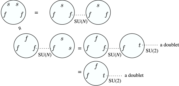
Figure 4: A sphere with punctures $f,f,s,s$ and two ways of decomposition. Every step is understood to be performed at finite area.

When $N=3$ the analysis can be stated more simply, since the puncture $t$ is the full puncture $f$. In this case, $\dim_{\mathbb{C}}\eta(C_{fss},\mathcal{A})=14$. The $\mathrm{SU}(3)$ action is broken to $\mathrm{SU}(2)$. Ten of the chiral multiplets give mass to the $5$ broken generators, leaving four chiral multiplets charged under $\mathrm{SU}(2)$, which is in fact in the doublet. So, we have $C_{fff}$ coupled to $C_{fss}$, via $\mathrm{SU}(3)$ gauge group. But this is spontaneously broken to $\mathrm{SU}(2)$ because of the property of $C_{fss}$, leaving a doublet of $\mathrm{SU}(2)$ in the $\mathcal{A}\to 0$ limit.

4.3 A sphere with four punctures of type $[k,k]$

As a final example, let $N=2k$ and consider a sphere with four punctures of type $[k,k]$. This is dual to $k$ D3-branes probing a $D_{4}$-type singularity, i.e. an orientifold 7-plane with four D7-branes on top of it. Therefore the 4d field content is $\mathrm{Sp}(k)$ with four fundamentals and one antisymmetric.

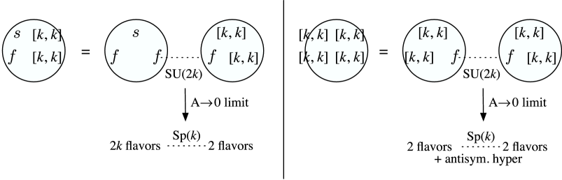
Figure 5: A sphere with punctures $f,s,[k,k],[k,k]$, and a sphere with four punctures of type $[k,k]$. The appearance of an additional antisymmetric in the second case can be understood naturally in our approach .

In [3, 29, 8], it was noted that a sphere with four punctures $f$, $s$ and two $[k,k]$’s realizes $\mathrm{Sp}(k)$ theory with $2k+2$ flavors, which is perturbatively conformal. By splitting the sphere, $2k$ flavors can be accounted for as coming from $C_{ffs}$, which gives $2k$ flavors of $\mathrm{SU}(2k)$. Then two punctures of type $[k,k]$ were thought of as somehow restricting the gauge group to be $\mathrm{Sp}(k)$, and moreover providing $2$ more flavors, see the left side of Fig. 5.

We interpret this as saying that the Higgs branch $X=\eta(C_{[k,k],[k,k],f})$ has an action of $\mathrm{SU}(2k)$ on the full puncture, but it is always broken to $\mathrm{Sp}(k)$. At a point where $\mathrm{Sp}(k)$ is preserved, one has two fundamentals. Then, if we glue this to $C_{ffs}$, the $\mathrm{SU}(2k)$ is spontaneously broken to $\mathrm{Sp}(k)$, and the directions of $X$ representing the broken directions in $\mathrm{SU}(2k)/\mathrm{Sp}(k)$ are eaten by the massive vector bosons.

Now, consider the sphere with four punctures of type $[k,k]$. This is obtained by gluing two copies of $C_{[k,k],[k,k],f}$ at the full puncture. Now, there is only one $\mathrm{SU}(2k)$ gauge group, which is broken to one $\mathrm{Sp}(k)$. However, we have two copies of manifold $X$, with two copies of broken directions $\mathrm{SU}(2k)/\mathrm{Sp}(k)$. Only one of them is eaten by the Higgs mechanism, and one remains as a physical direction, transforming as an antisymmetric of $\mathrm{Sp}(k)$. By taking the $\mathcal{A}\to 0$ limit, one finds $\mathrm{Sp}(k)$ theory with four flavors and an antisymmetric, as expected from the orientifold picture. In comparison, in the approach of [8], the appearance of the antisymmetric needs to be put in by hand.

5 OPE of Codimension-Two Defects

In this section we would like to use some of the lessons learned from the limits and compactifications we have studied to learn about the six-dimensional $(2,0)$ theory itself in $\mathbb{R}^{1,5}$. Namely, we can consider the behavior in $\mathbb{R}^{1,5}$ when two half-BPS codimension-two defects $D(\rho)$ are placed parallel to each other and are brought together. Suppose the transverse plane is identified with $\mathbb{C}$ and one defect sits at $z=0$ while the other is at a point $z$. What happens as $z\to 0$ ?

In order to answer this question it is necessary to enlarge the set of half-BPS defects under consideration. When $D(\rho)$ has global symmetry $H$ it can be coupled to any 4d N=2 field theory with $H$-global symmetry, say $T^{4}_{H}$, by gauging the diagonal global symmetry, as in (1.2). This gives a new defect

$$D(\rho,T^{4}_{H},q) :=D(\rho)\times_{H,q}T^{4}_{H}$$ (5.1)

$$=\int[d\Phi]e^{i2\pi\int d^{4}xd^{4}\theta\tau\mathrm{tr}\Phi^{2}/2+c.c.}T^{4}_{H}(\Phi)D(\rho;\Phi)$$ (5.2)

where $\Phi$ stands for the $\mathcal{N}=2$ vector superfield; $D(\rho;\Phi)$ and $T^{4}_{H}(\Phi)$ stand for the defect $D(\rho)$ and the theory $T^{4}_{H}$ coupled to the external vector superfield $\Phi$. In particular the lowest component of $\Phi$ serves as mass parameters for $D(\rho)$ and $T^{4}_{H}$. The path integral (5.2) then makes $\Phi$ dynamical, with coupling constant $\tau$.

To make this path integral UV complete, there is a bound on the flavor central charge $k$ of the global $H$ currents of the two components. Namely,

$$k(T^{4}_{H})+k(D(\rho))\leq k(\text{adjoint hyper of $H$}).$$ (5.3)

$k$ is proprotional to the contribution of the theory to the one-loop beta function of $H$ gauge fields [30, 31, 10]. When this equality is not saturated $e^{i\pi\tau}$ undergoes dimensional transmutation to a dimensionfull scale. Then, defects preserving the conformal invariance should saturate the bound if we want a 4d superconformal theory.

Suppose we have $D(\rho_{1})$ at $z=0$ and $D(\rho_{2})$ at $z$. Then, from far away, there should be an effective defect representing the two. We conjecture that it is of the type $D(\rho_{3},T^{4}_{H},q)$ where $q=z=e^{i\pi\tau}$. The precise rules for determining $\rho_{3}$ from $\rho_{1},\rho_{2}$ can be extracted from Section 4.5 of [3] and from [8]. We will see a few examples momentarily.

We can express this operation as

$$\begin{split}D(\rho_{1})_{z}D(\rho_{2})_{0}&\sim D(\rho_{3},T^{4}_{H},z)\\ &=\int[d\Phi]z^{S[\Phi]}\bar{z}^{S[\bar{\Phi}]}T^{4}_{H}(\Phi)D(\rho_{3};\Phi)\end{split}$$ (5.4)

where $S[\Phi]=2\pi\int d^{4}xd^{4}\theta\mathrm{tr}\Phi^{2}/2$.

Comparing this to the standard OPE $\mathcal{O}_{1}(z,\bar{z})\mathcal{O}_{2}(0)\sim\sum_{i}z^{\Delta_{i}}\bar{z}^{\bar{\Delta}_{i}}c^{i}_{12}O_{i}(0)$, we see that the conformal dimensions $\Delta_{i}$ are formally reinterpreted as the action of the vector multiplet $\Phi$, while the four-dimensional quantum field theory $T^{4}_{H}$ appears as an “operator product expansion coefficient.” Furthermore, it is a path integral, instead of a summation. The appearance of a four-dimensional field theory as an operator product expansion coefficient generalizes the vector-space-valued OPE coefficients of line defects discussed in [32]. We expect this idea will fit in naturally with the general ideas of extended topological field theories currently under development by several physical mathematicians.

For examples, we can rewrite what we learned in Sec. 4 in the language of the OPE. The analysis of $C_{fss}$ leads us to the equality (4.5) in Sec. 4.2. This can be though of as the OPE

$$D(s)_{z}D(s)_{0}\sim D(t,(\text{one flavor})_{\mathrm{SU}(2)},z),$$ (5.5)

where $(\text{one flavor})_{\mathrm{SU}(2)}$ stands for the theory of free hypermultiplets in the doublet of $\mathrm{SU}(2)$. Similarly the analysis of $C_{f,[k,k],[k,k]}$ in Sec. 4.3 tells us that

$$D([k,k])_{z}D([k,k])_{0}\sim D(f,(\text{two flavors})_{\mathrm{Sp}(k)},z).$$ (5.6)

In this language, the sphere with four punctures of type $[k,k]$ can be analyzed as follows. First, we take the OPE of the two pairs using (5.6). Then, we have a sphere with two defects of type $D(f,(\text{two flavors})_{\mathrm{Sp}(k)},z)=D(f)\times_{\mathrm{Sp}(k)}(\text{two flavors})$. Equivalently, we have a sphere with two full punctures, each coupled to two flavors via $\mathrm{Sp}(k)$. The sphere with two full punctures produces a theory with Higgs branch $I(\mathcal{A})=T^{*}\mathrm{SU}(2k)_{\mathbb{C}}$. We are gauging this theory via $\mathrm{Sp}(k)^{2}$ from the left and the right simultaneously. This breaks $\mathrm{Sp}(k)^{2}$ to $\mathrm{Sp}(k)$, and a part of $I(\mathcal{A})$ remains as the antisymmetric of $\mathrm{Sp}(k)$. Taking $\mathcal{A}\to 0$ limit, we have 4d $\mathrm{Sp}(k)$ theory coupled to four flavors plus an antisymmetric.

References

- [1] A. Klemm, W. Lerche, P. Mayr, C. Vafa, and N. P. Warner, “Self-Dual Strings and Supersymmetric Field Theory,” Nucl. Phys. B477 (1996) 746–766, arXiv:hep-th/9604034.
- [2] E. Witten, “Solutions of four-dimensional field theories via M theory,” Nucl.Phys. B500 (1997) 3–42, arXiv:hep-th/9703166 [hep-th].
- [3] D. Gaiotto, “ Dualities,” arXiv:0904.2715 [hep-th].
- [4] D. Gaiotto, G. W. Moore, and A. Neitzke, “Wall-Crossing, Hitchin Systems, and the WKB Approximation,” arXiv:0907.3987 [hep-th].
- [5] M. T. Anderson, C. Beem, N. Bobev, and L. Rastelli, “Holographic Uniformization,” arXiv:1109.3724 [hep-th].
- [6] D. Gaiotto and E. Witten, “S-Duality of Boundary Conditions in Super Yang-Mills Theory,” arXiv:0807.3720 [hep-th].
- [7] G. W. Moore and Y. Tachikawa, “On 2D TQFTs whose Values are Holomorphic Symplectic Varieties,” arXiv:1106.5698 [hep-th].
- [8] O. Chacaltana and J. Distler, “Tinkertoys for Gaiotto Duality,” JHEP 11 (2010) 099, arXiv:1008.5203 [hep-th].
- [9] O. Chacaltana and J. Distler, “Tinkertoys for the Series,” arXiv:1106.5410 [hep-th].
- [10] P. C. Argyres and N. Seiberg, “S-Duality in Supersymmetric Gauge Theories,” JHEP 12 (2007) 088, arXiv:0711.0054 [hep-th].
- [11] F. Benini, Y. Tachikawa, and D. Xie, “Mirrors of 3D Sicilian Theories,” JHEP 09 (2010) 063, arXiv:1007.0992 [hep-th].
- [12] D. Gaiotto and J. Maldacena, “The Gravity Duals of Superconformal Field Theories,” arXiv:0904.4466 [hep-th].
- [13] S. A. Cherkis, “Moduli Spaces of Instantons on the Taub-Nut Space,” Commun. Math. Phys. 290 (2009) 719–736, arXiv:0805.1245 [hep-th].
- [14] S. A. Cherkis, “Instantons on the Taub-Nut Space,” Adv. Theor. Math. Phys. 14 (2010) 609–642, arXiv:0902.4724 [hep-th].
- [15] S. A. Cherkis, “Instantons on Gravitons,” Commun. Math. Phys. 306 (2011) 449–483, arXiv:1007.0044 [hep-th].
- [16] C. D. A. Blair and S. A. Cherkis, “One Monopole with Singularities,” JHEP 11 (2010) 127, arXiv:1009.5387 [hep-th].
- [17] C. D. A. Blair and S. A. Cherkis, “Singular Monopoles from Cheshire Bows,” Nucl. Phys. B845 (2011) 140–164, arXiv:1010.0740 [hep-th].
- [18] S. A. Cherkis, C. O’Hara, and C. Sämann, “Super Yang-Mills Theory with Impurity Walls and Instanton Moduli Spaces,” Phys. Rev. D83 (2011) 126009, arXiv:1103.0042 [hep-th].
- [19] P. B. Kronheimer, “A hyperkähler structure on the cotangent bundle of a complex Lie group,” MSRI preprint (1988) , arXiv:math.DG/0409253.
- [20] R. Bielawski, “Hyperkähler structures and group actions,” J. London Math. Soc. 55 (1997) 400.
- [21] R. Bielawski, “Lie groups, Nahm’s equations and hyperkähler manifolds,” in Algebraic Groups, Y. Tschinkel, ed. Universitätsdrucke Göttingen, 2005. arXiv:math.DG/0509515.
- [22] D. Gaiotto and E. Witten, “Supersymmetric Boundary Conditions in Super Yang-Mills Theory,” arXiv:0804.2902 [hep-th].
- [23] F. Benini, Y. Tachikawa, and B. Wecht, “Sicilian Gauge Theories and Dualities,” JHEP 01 (2010) 088, arXiv:0909.1327 [hep-th].
- [24] D. M. Hofman and J. Maldacena, “Conformal Collider Physics: Energy and Charge Correlations,” JHEP 05 (2008) 012, arXiv:0803.1467 [hep-th].
- [25] A. D. Shapere and Y. Tachikawa, “Central Charges of Superconformal Field Theories in Four Dimensions,” JHEP 09 (2008) 109, arXiv:0804.1957 [hep-th].
- [26] A. Dancer and A. Swann, “Non-Abelian Cut Constructions and hyperkähler Modifications,” arXiv:1002.1837 [math.DG].
- [27] S. Alexandrov, B. Pioline, F. Saueressig, and S. Vandoren, “Linear Perturbations of Quaternionic Metrics - I. the hyperkähler Case,” Lett. Math. Phys. 87 (2009) 225–265, arXiv:0806.4620 [hep-th].
- [28] D. Gaiotto, A. Neitzke, and Y. Tachikawa, “Argyres-Seiberg Duality and the Higgs Branch,” Commun. Math. Phys. 294 (2010) 389–410, arXiv:0810.4541 [hep-th].
- [29] D. Nanopoulos and D. Xie, “ SU Quiver with USp ends or SU ends with antisymmetric matter,” JHEP 08 (2009) 108, arXiv:0907.1651 [hep-th].
- [30] J. Erdmenger and H. Osborn, “Conserved currents and the energy momentum tensor in conformally invariant theories for general dimensions,” Nucl.Phys. B483 (1997) 431–474, arXiv:hep-th/9605009 [hep-th].
- [31] D. Anselmi, “Central functions and their physical implications,” JHEP 9805 (1998) 005, arXiv:hep-th/9702056 [hep-th].
- [32] D. Gaiotto, G. W. Moore, and A. Neitzke, “Framed BPS States,” arXiv:1006.0146 [hep-th].