Elmar P. Biernat
Quantization on
Space-Time Hyperboloids
Diplomarbeit
zur Erlangung des akademischen Grades eines
Magisters
an der Naturwissenschaften Fakultät der
Karl-Franzens-Universität Graz
Betreuer:
Ao. Univ.-Prof. Dr. Wolfgang Schweiger
Institut für Physik, Fachbereich Theoretische Physik
September 2007

Für Justine

Abstract

We quantize a relativistic massive complex spin-$0$ field and a relativistic massive spin-$\frac{1}{2}$ field on a space-time hyperboloid. We call this procedure point-form canonical quantization. Lorentz invariance of the hyperboloid implies that the 4 generators for translations become dynamic and interaction dependent, whereas the 6 generators for Lorentz transformations remain kinematic and interaction free. We expand the fields in terms of usual plane waves and prove the equivalence to equal-time quantization by representing the Poincaré generators in a momentum basis. We formulate a generalized scattering theory for interacting fields by considering evolution of the system generated by the interaction dependent four-momentum operator. Finally we expand our generalized scattering operator in powers of the interaction and show its equivalence to the Dyson expansion of usual time-ordered perturbation theory.

Contents

1. 1 Introduction and Overview
2. 2 Fundamentals of Quantum Field Theory
   1. 2.1 Poincaré Group
   2. 2.2 Fields
      1. 2.2.1 Transformation Laws
      2. 2.2.2 Noether Theorem
      3. 2.2.3 Microscopic Causality
      4. 2.2.4 Fock Space
      5. 2.2.5 Scattering Operator
3. 3 Time Parameterization
   1. 3.1 Free Relativistic Particle
      1. 3.1.1 Singular System
      2. 3.1.2 Reparameterization Invariance
      3. 3.1.3 Space-Time Foliation
   2. 3.2 Forms of Relativistic Dynamics
      1. 3.2.1 Instant Form
      2. 3.2.2 Front Form
      3. 3.2.3 Point Form
   3. 3.3 General Evolution
4. 4 Covariant Canonical Quantization of Free Fields
   1. 4.1 Complex Klein-Gordon Fields
      1. 4.1.1 Invariant Scalar Product
      2. 4.1.2 Covariant Canonical Commutation Relations
      3. 4.1.3 Commutation Relations in Momentum Space
      4. 4.1.4 Generators in Wigner Representation
   2. 4.2 Dirac Fields
      1. 4.2.1 Invariant Scalar Product
      2. 4.2.2 Covariant Canonical Anticommutation Relations
      3. 4.2.3 Anticommutation Relations in Momentum Space
      4. 4.2.4 Generators in Wigner Representation
5. 5 Covariant Scattering Theory for Interacting Fields
   1. 5.1 Poincaré Generators
   2. 5.2 Covariant Interaction Picture
   3. 5.3 Lorentz-Invariant Scattering Operator
6. 6 Summary and Outlook
7. A Hypersurface Element
8. B $W$ and $W^{\mu}$ Distribution
   1. B.1 $W$ Distribution
   2. B.2 $W^{\mu}$ Distribution
9. C Complex Klein-Gordon Fields
   1. C.1 Pauli-Jordan Function
   2. C.2 Covariant Canonical Commutation Relations
   3. C.3 Commutation Relations in Momentum Space
   4. C.4 Generators in Wigner Representation
      1. C.4.1 Generator for Global Gauge Transformations
      2. C.4.2 Translation Generator
10. D Dirac Fields
    1. D.1 Invariant Scalar Product
    2. D.2 Covariant Canonical Anticommutation Relations
    3. D.3 Anticommutation Relations in Momentum Space
    4. D.4 Generators in Wigner Representation
       1. D.4.1 Generator for Global Gauge Transformations
       2. D.4.2 Translation Generator
11. E Dyson Expansion
    1. E.1 First Order
    2. E.2 Second Order
    3. E.3 Third Order

Chapter 1 Introduction and Overview

With his theory of relativity Einstein replaced the absolute character of space and time in Newtonian mechanics by giving them a relative meaning. In Newtonian physics the three-dimensional physical space and the one-dimensional time are represented separately by the three-dimensional Euclidean space and the real numbers, respectively. In special relativity space and time are treated equally, forming the combined notion of space-time represented by the four-dimensional Minkowski space. On the other hand, classical mechanics was replaced by the quantum theory of Schrödinger and Heisenberg, treating the space observable as operator and leaving time as a c-number parameter.
In order to make quantum theory consistent with the theory of special relativity Dirac and others initiated what is known as relativistic quantum mechanics. In his famous paper Forms of Relativistic Dynamics [1] Dirac found a way to make the Poincaré group applicable to quantum theory. Furthermore, he pointed out the possibility of formulating Poincaré invariant relativistic dynamics in different ways, depending on the foliation of Minkowski space. He found three forms: the instant, front and point form. Each form corresponds to a different choice of a spacelike hypersurface defining an instant in the time parameter. This hypersurface is invariant under the action of certain Poincaré generators (kinematic generators) which span the, so called, stability group. The others, the dynamic generators, generate evolution of the system and contain interactions (if present) whereas the kinematic generators stay interaction free. Therefore each form describes a different way of including interactions into the free theory.
Inconsistencies of relativistic quantum mechanics with the existence of anti-particles and relativistic causality can be resolved by going from a finite number of degrees of freedom to infinitely many degrees of freedom. This corresponds to setting up a local quantum field theory. The arbitrariness of choosing a time parameter will still be present in a quantum field theory and is reflected in the arbitrariness of the choice of hypersurface on which canonical (anti)commutation relations are imposed. This issue was taken up by Tomonaga [2] and Schwinger [3] by formulating generalized canonical (anti)commutation relations on arbitrary spacelike hypersurfaces.
Field quantization on the Lorentz-invariant forward hyperboloid $x_{\lambda}\,x^{\lambda}=\tau^{2}$, with $\tau$ arbitrary but fixed, provides a simple example of field quantization on a curved hypersurface. Following Dirac’s nomenclature [1] we speak in this context of point-form quantum field theory. Due to the curvilinear nature of the hyperboloid field quantization is not straightforward. Therefore only a few papers exist about point-form quantum field theory [4, 5, 6, 7, 8] and they mainly don’t go beyond free fields. Most of these attempts to quantize field theories on the hyperboloid made use of hyperbolic coordinates. The “Hamiltonian” in these coordinates is identified with the generator for dilatation transformations, which is explicitly “hyperbolic-time” dependent and does not belong to the Poincaré group. Furthermore, it is first only defined in the forward light cone. This restriction can be overcome by analytical continuation, although it does not seem very convenient to consider development in hyperbolic time, especially if one wants to describe scattering. The field equations in these coordinates are solved in terms of Hankel functions. The associated field quanta are characterized by the eigenvalues of the generators for Lorentz boosts, which become diagonal in the corresponding Fock representation (Lorentz basis). However, the definition of the translation generator as a self-adjoint operator acting on square integrable functions of these boost eigenvalues is not completely straightforward [9]. Altogether, these approaches do not seem to be very useful for massive theories and lead to difficulties in describing scattering.

In this thesis we argue that it is more convenient to work with the usual Cartesian coordinates and to expand the fields in terms of usual plane waves. The associated field quanta are characterized by the eigenvalues of the three-momentum operator and a spin number. The four-momentum operator represented in this Wigner basis becomes diagonal. Moreover, a Lorentz-invariant formulation of scattering can be easily achieved by considering evolution generated by the four-momentum operator.

In point-form quantum mechanics, many ideas for the construction of interaction potentials and current operators are motivated by quantum field theoretical considerations. This emphasizes the necessity of formulating an interacting point-form quantum field theory. Furthermore, point-form quantum field theory can be viewed as a special case of field quantization in curved space-time, that is, with a classical gravitational background [10, 11]. Altogether, this should provide enough motivation for setting up a point-form quantum field theory.

In Chapter 2 some basics of quantum field theory and an overview of its symmetries are given, which will be frequently used and referred to in the following chapters. The topic of Chapter 3 is the problem of time parameterization. Invariance under reparameterization is a typical feature of parameterized Hamiltonian systems. This is first discussed for the classical free relativistic particle and then Dirac’s forms of relativistic dynamics are introduced. In Chapter 4 a free complex massive scalar field and a free massive spinor field are quantized on the hyperboloid by means of Lorentz-invariant (anti)commutation relations. Furthermore, the equivalence between instant- and point-form quantization of free fields is proved by using the Wigner representation of the Poincaré group. Finally, in Chapter 5, a manifest covariant formulation of scattering is presented. This leads to the same series expansion of a corresponding scattering operator as usual time-ordered perturbation theory does. All the longer calculations are put into five Appendices A, B, C, D and E.

Chapter 2 Fundamentals of Quantum Field Theory

In this chapter we give an overview of the basic theorems and definitions of quantum field theory, which will be frequently used and referred to throughout the thesis.

2.1 Poincaré Group

In his paper [12] Wigner realized that the fundamental symmetry group of a relativistic quantum theory is the Poincaré group $\mathcal{P}$ of special relativity. It is the group of all transformations of Minkowski space-time that leave the distance between 2 points invariant. It can be written as the semi-direct product of $\mathbb{R}^{4}$ with the Lorentz group $\mathcal{L}$. We will restrict ourselves to the restricted Poincaré group $\mathcal{P}_{+}^{\uparrow}$ being the group of space-time translations together with rotations and boosts. Its elements, denoted by a pair $(a,\Lambda)$ with $a\in\mathbb{R}^{4}$ and $\Lambda\in\mathcal{L}_{+}^{\uparrow}$, form a ten-dimensional Lie group. Its parameters are the four-vector $a^{\mu}$ and the skew-symmetric, real $\omega^{\mu\nu}$. An operator representation of infinitesimal $\mathcal{P}_{+}^{\uparrow}$ transformations which act on scalar functions of Minkowski space-time is given by[14]

$$\Omega\left(a,\Lambda\right)=\mathbf{1}+ia^{\lambda}\,P_{\lambda}-\frac{i}{2}\omega^{\lambda\sigma}\,M_{\lambda\sigma}+\mathcal{O}\left(a^{2},\omega^{2}\right),$$ (2.1)

where $M^{\mu\nu}=-M^{\nu\mu}$. The operators $P^{\mu}$ and $M^{\mu\nu}$ are then given by

$$P^{\mu} = i\frac{\partial}{\partial x_{\mu}},$$ (2.2)

$$M^{\mu\nu} = x^{\mu}P^{\nu}-x^{\nu}P^{\mu},\quad\text{with}\quad x\in\mathbb{R}^{4}.$$ (2.3)

They satisfy the following commutation relations of the Lie algebra of $\mathcal{P}$:

$$\left[P^{\mu},P^{\nu}\right] = 0,$$ (2.4)

$$\left[M^{\mu\nu},P^{\rho}\right] = i\left(g^{\nu\rho}P^{\mu}-g^{\mu\rho}P^{\nu}\right),$$ (2.5)

$$\left[M^{\mu\nu},M^{\lambda\sigma}\right] = -i\left(g^{\mu\lambda}M^{\nu\sigma}-g^{\nu\lambda}M^{\mu\sigma}+g^{\nu\sigma}M^{\mu\lambda}-g^{\mu\sigma}M^{\nu\lambda}\right).$$ (2.6)

Only these commutation relations are essential for the definition of the Lie algebra, they are satisfied for any arbitrary representation of $\mathcal{P}_{+}^{\uparrow}$. $P^{\mu}$ and $M^{\mu\nu}$ are called generators of $\mathcal{P}_{+}^{\uparrow}$, they generate space-time translations and Lorentz transformations parameterized by $a$ and $\omega$, respectively. Since the proper Lorentz group has covering group $SL\left(2,\mathbb{C}\right)$, we shall call the covering group of the $\mathcal{P}_{+}^{\uparrow}$ inhomogeneous $SL\left(2,\mathbb{C}\right)$.

2.2 Fields

All relativistic theories should be invariant under $\mathcal{P}_{+}^{\uparrow}$. For relativistic quantum theories there is a physical Hilbert space $\mathcal{H}$ in which a unitary representation $\hat{U}\left(a,\Lambda\right)$ of the inhomogeneous $SL\left(2,\mathbb{C}\right)$ acts, giving the relativistic transformation law of the states. $\hat{U}\left(a,\mathbf{1}\right)$ can be written as $\hat{U}\left(a,\mathbf{1}\right)=\mathrm{e}^{ia_{\lambda}\,\hat{P}^{\lambda}}$ with $\hat{P}^{\lambda}$ unbounded and hermitian. The operator $\hat{P}_{\lambda}\,\hat{P}^{\lambda}=\hat{M}^{2}$ is interpreted as the square of the mass and the eigenvalues of $\hat{P}^{\mu}$ lie in or on the forward light cone.

2.2.1 Transformation Laws

Let us consider classical fields $\chi_{\alpha}\left(x\right)$ that transform under a Poincaré transformation $(a,\Lambda)$ as

$$\chi_{\alpha}\left(x\right)\rightarrow\chi_{\alpha}^{\prime}\left(x^{\prime}\right)=S\left(\Lambda\right)_{\alpha}^{~{}\beta}\chi_{\beta}\left(x\right),\quad x^{\prime}=\Lambda x+a.$$ (2.7)

After quantization the classical fields $\chi_{\alpha}\left(x\right)$ are replaced by field operators $\hat{\chi}_{\alpha}\left(x\right)$ that act on a Hilbert space $\mathcal{H}$. Quantum states $|\Phi\rangle$, which are elements of $\mathcal{H}$, behave under Poincaré transformations like

$$\mathcal{H}\ni|\Phi\rangle\rightarrow|\Phi^{\prime}\rangle=\hat{U}\left(a,\Lambda\right)|\Phi\rangle\in\mathcal{H},$$ (2.8)

with $\hat{U}\left(a,\Lambda\right)$ being a unitary operator. The classical fields $\chi_{\alpha}\left(x\right)$ correspond to expectation values of the field operators $\hat{\chi}_{\alpha}\left(x\right)$ $\langle\Phi|\hat{\chi}_{\alpha}\left(x\right)|\Phi\rangle$ and the transformed fields $\chi^{\prime}_{\alpha}\left(x^{\prime}\right)$ correspond to a transformed matrix element $\left\langle\Phi^{\prime}\left|\hat{\chi}_{\alpha}\left(x^{\prime}\right)\right|\Phi^{\prime}\right\rangle$. From (2.7) and (2.8) we find

$$S\left(\Lambda\right)_{\alpha}^{~{}\beta}\langle\Phi|\hat{\chi}_{\beta}\left(x\right)|\Phi\rangle=\langle\Phi|\,\hat{U}\left(a,\Lambda\right)^{-1}\hat{\chi}_{\alpha}\left(x^{\prime}\right)\hat{U}\left(a,\Lambda\right)|\Phi\rangle.$$ (2.9)

This equation is valid for arbitrary states, therefore a field operator transforms under $\hat{U}\left(a,\Lambda\right)$ as

$$\hat{U}\left(a,\Lambda\right)\hat{\chi}_{\alpha}\left(x\right)\hat{U}\left(a,\Lambda\right)^{-1}=S\left(\Lambda^{-1}\right)_{\alpha}^{~{}\beta}\hat{\chi}_{\beta}\left(\Lambda x+a\right).$$ (2.10)

For a spin-0 field operator $\hat{\phi}$ (Lorentz scalar) we have then

$$\hat{U}\left(a,\Lambda\right)\hat{\phi}\left(x\right)\hat{U}\left(a,\Lambda\right)^{-1}=\hat{\phi}\left(\Lambda x+a\right).$$ (2.11)

For a spin-$\frac{1}{2}$ field operator $\hat{\psi}$ (Lorentz four-spinor) we have for the components $\hat{\psi}_{\alpha},\,\alpha=1,\ldots 4$

$$\hat{U}\left(a,\Lambda\right)\hat{\psi}_{\alpha}\left(x\right)\hat{U}\left(a,\Lambda\right)^{-1}=S\left(\Lambda^{-1}\right)_{\alpha}^{~{}\beta}\hat{\psi}_{\beta}\left(\Lambda x+a\right),$$ (2.12)

where $S\left(\Lambda^{-1}\right)$ is a $4\times 4$-matrix representation of the $SL\left(2,\mathbb{C}\right)$[15].

2.2.2 Noether Theorem

A symmetry of a theory is equivalent with the invariance of the action under a certain transformation. According to Neother’s theorem, every symmetry of the action corresponds to an integral of motion of the theory. The classical action is given by

$$S\left[\chi\right]:=\int_{\mathbb{R}^{4}}\mathrm{d}^{4}x\,\mathcal{L}\left(\chi_{\alpha}\left(x\right),\partial_{\mu}\chi_{\alpha}\left(x\right)\right),$$ (2.13)

with the Lagrangian density $\mathcal{L}\left(\chi_{\alpha}\left(x\right),\partial_{\mu}\chi_{\alpha}\left(x\right)\right)$ being a function of the fields and their first derivatives. The Hamiltonian principle of making the action stationary gives the Euler-Lagrange equations as

$$\frac{\delta S}{\delta\chi_{\alpha}\left(x\right)}=\frac{\partial\mathcal{L}}{\partial\chi_{\alpha}\left(x\right)}-\partial_{\mu}\left(\frac{\partial\mathcal{L}}{\partial\left(\partial_{\mu}\chi_{\alpha}\left(x\right)\right)}\right)\stackrel{{\scriptstyle!}}{{=}}0,$$ (2.14)

where $\frac{\delta}{\delta\chi\left(x\right)}$ denotes the functional differentiation.
Let us now consider an infinitesimal symmetry transformation of the form

$$\chi_{\alpha}\left(x\right)\rightarrow\chi^{\prime}_{\alpha}\left(x\right)=\chi_{\alpha}\left(x\right)+\epsilon T_{\alpha}\left(\chi_{1}\left(x\right),\chi_{2}\left(x\right),\ldots\right).$$ (2.15)

Remarkably, the integral of motion $G$, associated with this symmetry transformation, is its infinitesimal generator in the sense that

$$T_{\alpha}\left(\chi_{1}\left(x\right),\chi_{2}\left(x\right),\ldots\right)=\left\{\chi_{\alpha}\left(x\right),G\right\}_{P},$$ (2.16)

where $\left\{\ldots\right\}_{P}$ denotes the Poisson bracket. For field operators $\hat{\chi}_{\alpha}$ the Poisson bracket is replaced by the commutator

$$T_{\alpha}\left(\hat{\chi}_{1}\left(x\right),\hat{\chi}_{2}\left(x\right),\ldots\right)=\left[i\hat{G},\hat{\chi}_{\alpha}\left(x\right)\right].$$ (2.17)

Global Gauge Transformations

We assume that the action and even the Lagrangian density of a complex field is invariant under a global $U\left(1\right)$ phase transformation, i.e.

$$\delta\mathcal{L}\left(x\right):=\mathcal{L}\left(\chi^{\prime}\left(x\right),\partial_{\mu}\chi^{\prime}\left(x\right)\right)-\mathcal{L}\left(\chi\left(x\right),\partial_{\mu}\chi\left(x\right)\right)\stackrel{{\scriptstyle!}}{{=}}0,$$ (2.18)

$$\text{if}\quad\chi^{\prime}\left(x\right)=\mathrm{e}^{-i\epsilon}\chi\left(x\right)\quad\text{and}\quad\chi^{\prime\ast}\left(x\right)=\mathrm{e}^{i\epsilon}\chi^{\ast}\left(x\right),\quad\epsilon=\mathrm{const.}\quad.$$ (2.19)

With the help of $\delta\left(\partial_{\mu}\chi\right)=\partial_{\mu}\left(\delta\chi\right)$ and (2.14) we find for infinitesimal transformations that

$$\delta\mathcal{L}\left(x\right)=\partial_{\mu}\left[\frac{\partial\mathcal{L}\left(x\right)}{\partial\left(\partial_{\mu}\chi\left(x\right)\right)}\delta\chi\left(x\right)\right]+\partial_{\mu}\left[\frac{\partial\mathcal{L}\left(x\right)}{\partial\left(\partial_{\mu}\chi^{\ast}\left(x\right)\right)}\delta\chi^{\ast}\left(x\right)\right]=0,$$ (2.20)

where

$$\delta\chi\left(x\right):=\chi^{\prime}\left(x\right)-\chi\left(x\right)\approx-i\epsilon\chi\left(x\right)\quad\text{and}\quad\delta\chi^{\ast}\left(x\right)\approx i\epsilon\chi^{\ast}\left(x\right)$$ (2.21)

are the variations of $\chi\left(x\right)$ and $\chi^{\ast}\left(x\right)$ at point $x$. Then the quantity in the square brackets in (2.20) is a conserved symmetry current

$$\partial_{\mu}\,\mathcal{J}^{\mu}\left(x\right)=0,\quad\text{with}\quad\mathcal{J}^{\mu}\left(x\right):=i\frac{\partial\mathcal{L}\left(x\right)}{\partial\left(\partial_{\mu}\chi\left(x\right)\right)}\chi\left(x\right)-i\frac{\partial\mathcal{L}\left(x\right)}{\partial\left(\partial_{\mu}\chi^{\ast}\left(x\right)\right)}\chi^{\ast}\left(x\right).$$

This current integrated over a spacelike hypersurface gives a conserved charge

$$Q=\int_{\Sigma}\mathrm{d}\Sigma^{\mu}\left(x\right)\mathcal{J}_{\mu}\left(x\right),$$ (2.23)

with $\mathrm{d}\Sigma^{\mu}\left(x\right)$ denoting the oriented hypersurface element. In a quantum field theory, $Q$ becomes an operator $\hat{Q}$ generating global gauge transformations  (2.21) in the sense that

$$\hat{\chi}\left(x\right)=\left[\hat{\chi}\left(x\right),\hat{Q}\right],\quad\hat{\chi}^{{\dagger}}\left(x\right)=-\left[\hat{\chi}^{{\dagger}}\left(x\right),\hat{Q}\right].$$ (2.24)

Translations

Let the Lagrangian density $\mathcal{L}\left(x\right)$ be form invariant, i.e. $\mathcal{L}^{\prime}\left(x^{\prime}\right)=\mathcal{L}\left(x\right)$, under a translation $x^{\prime}=x+a$ that transforms the fields as

$$\chi_{\alpha}\left(x\right)\rightarrow\chi^{\prime}_{\alpha}\left(x^{\prime}\right)=\chi_{\alpha}\left(x\right).$$ (2.25)

Again it is sufficient to consider infinitesimal displacements. The variation of the fields and their derivatives at the point $x$ is then

$$\delta\chi_{\alpha}\left(x\right) := \chi_{\alpha}^{\prime}\left(x\right)-\chi_{\alpha}\left(x\right)=a^{\nu}\partial_{\nu}\chi_{\alpha}\left(x\right),$$ (2.26)

$$\delta\partial_{\mu}\chi_{\alpha}\left(x\right) = \partial_{\mu}\delta\chi_{\alpha}\left(x\right).$$ (2.27)

Expansion in the small parameters $a^{\nu}$ gives for the change in the Lagrangian density (at point $x$)

$$\delta\mathcal{L}\left(x\right)=a^{\nu}\partial_{\nu}\mathcal{L}\left(x\right).$$ (2.28)

On the other hand we get from (2.18) with the help of (2.26), (2.27) and (2.14)

$$\delta\mathcal{L}\left(x\right)=\partial_{\mu}\left(\frac{\partial\mathcal{L}\left(x\right)}{\partial\left(\partial_{\mu}\chi_{\alpha}\left(x\right)\right)}a^{\nu}\partial_{\nu}\chi_{\alpha}\left(x\right)\right).$$ (2.29)

Since $a$ is arbitrary, we get from comparison of (2.28) and (2.29)

$$\partial_{\mu}\left[\frac{\partial\mathcal{L}\left(x\right)}{\partial\left(\partial_{\mu}\chi_{\alpha}\left(x\right)\right)}\partial_{\nu}\chi_{\alpha}\left(x\right)-g^{\mu}_{\nu}\mathcal{L}\left(x\right)\right]=0.$$ (2.30)

The quantity in the square brackets is a conserved Noether current called energy-momentum tensor

$$\mathcal{T}^{\mu}_{\nu}\left(x\right):=\frac{\partial\mathcal{L}\left(x\right)}{\partial\left(\partial_{\mu}\chi_{\alpha}\left(x\right)\right)}\partial_{\nu}\chi_{\alpha}\left(x\right)-g^{\mu}_{\nu}\mathcal{L}\left(x\right).$$ (2.31)

At this point it is important to note for later purposes, that this expression is valid for both interacting theories and free theories. If the interaction terms in $\mathcal{L}$ do not contain derivatives of the fields, all interaction terms are included in the second part only.
Integration of (2.31) over a spacelike hypersurface gives the four-momentum

$$P^{\mu}=\int_{\Sigma}\mathrm{d}\Sigma^{\nu}\left(x\right)\mathcal{T}^{\mu}_{\nu}\left(x\right).$$ (2.32)

In a quantum field theory $P^{\mu}$ becomes an operator $\hat{P}^{\mu}$ generating space-time translations of the field operator in the sense that

$$\partial^{\mu}\hat{\chi}\left(x\right)=i\left[\hat{P}^{\mu},\hat{\chi}\left(x\right)\right].$$ (2.33)

Lorentz Transformations

We consider an infinitesimal Lorentz transformation

$$\Lambda^{\mu}_{~{}\nu}=\delta^{\mu}_{~{}\nu}+\omega^{\mu}_{~{}\nu},$$ (2.34)

with a corresponding matrix representation of the $SL\left(2,\mathbb{C}\right)$ (cf. (2.10))

$$S\left(\Lambda\right)^{\alpha}_{~{}\beta}=\delta^{\alpha}_{~{}\beta}-\frac{i}{2}\omega_{\mu\nu}\left(S^{\mu\nu}\right)^{\alpha}_{~{}\beta}.$$ (2.35)

The fields transform according to (2.7) as

$$\chi^{\prime\alpha}\left(x^{\prime}\right)=S\left(\Lambda\right)^{\alpha}_{~{}\beta}\chi^{\beta}\left(x\right).$$ (2.36)

A Taylor expansion of the left hand side yields

$$\chi^{\prime\alpha}\left(x^{\prime}\right)=\left[1+\frac{1}{2}\omega^{\lambda\sigma}\left(x_{\lambda}\partial_{\sigma}-x_{\sigma}\partial_{\lambda}\right)\right]\chi^{\prime\alpha}\left(x\right)+\mathcal{O}\left(\omega^{2}\right).$$ (2.37)

The difference $\delta\chi^{\prime\alpha}\left(x\right)=\chi^{\prime\alpha}\left(x\right)-\chi^{\alpha}\left(x\right)$ is then

$$\delta\chi^{\alpha}\left(x\right)=-\frac{i}{2}\omega^{\lambda\sigma}\left[\left[S_{\lambda\sigma}\right]^{\alpha}_{~{}\beta}+L_{\lambda\sigma}\delta^{\alpha}_{~{}\beta}\right]\chi^{\beta}\left(x\right),$$ (2.38)

where $L_{\lambda\sigma}:=i\left(x_{\lambda}\partial_{\sigma}-x_{\sigma}\partial_{\lambda}\right)$. Similarly, we can write the variation of the derivative of the field as

$$\delta\partial_{\mu}\chi^{\alpha}\left(x\right)=-\frac{i}{2}\omega^{\lambda\sigma}\left[\left[S_{\lambda\sigma}\right]^{\alpha}_{~{}\beta}+L_{\lambda\sigma}\delta^{\alpha}_{~{}\beta}\right]\partial_{\mu}\chi^{\beta}\left(x\right)-\omega_{\mu}^{~{}\sigma}\partial_{\sigma}\chi^{\beta}\left(x\right).$$ (2.39)

We assume $\mathcal{L}$ to be form invariant under the Lorentz transformations (2.38) and (2.39). On using (2.14), (2.31) and integration by parts we get

$$i\partial_{\mu}\left[\frac{\partial\mathcal{L}}{\partial\left(\partial_{\mu}\chi^{\alpha}\right)}\left[S_{\lambda\sigma}\right]_{~{}\beta}^{\alpha}\chi^{\beta}\right]-\mathcal{T}_{\lambda\sigma}+\mathcal{T}_{\sigma\lambda}=0.$$ (2.40)

Since the conservation law (2.30) does not define the current in a unique way, we can always add a divergence of a total antisymmetric tensor $\mathcal{A}^{\lambda\mu\nu}$ satisfying the same conservation law. For symmetric $\mathcal{T}^{\mu\nu}$ we may construct the angular-momentum density as [16]

$$\mathcal{M}^{\mu\nu\sigma}\left(x\right):=x^{\nu}\mathcal{T}^{\mu\sigma}\left(x\right)-x^{\sigma}\mathcal{T}^{\mu\nu}\left(x\right),$$ (2.43)

conserved in the sense that

$$\partial_{\mu}\mathcal{M}^{\mu\nu\sigma}\left(x\right)=0.$$ (2.44)

Then the corresponding conserved charge is the integral over a spacelike hypersurface

$$M^{\mu\nu}=\int_{\Sigma}\mathrm{d}\Sigma_{\lambda}\left(x\right)\mathcal{M}^{\lambda\mu\nu}\left(x\right).$$ (2.45)

The antisymmetric tensor $M^{\mu\nu}$ becomes an operator $\hat{M}^{\mu\nu}$ in a quantum field theory generating Lorentz transformations of the field operator, i.e. Lorentz boosts and spatial rotations in the sense that

$$\left[\left(x^{\mu}\partial^{\nu}-x^{\nu}\partial^{\mu}\right)\delta^{\alpha}_{~{}\beta}-i\left[S^{\mu\nu}\right]^{\alpha}_{~{}\beta}\right]\hat{\chi}^{\beta}\left(x\right) = -i\left[L^{\mu\nu}\delta^{\alpha}_{~{}\beta}+\left[S^{\mu\nu}\right]^{\alpha}_{~{}\beta}\right]\hat{\chi}^{\beta}\left(x\right)$$ (2.46)

$$= i\left[\hat{\chi}^{\alpha}\left(x\right),\hat{M}^{\mu\nu}\right].$$

2.2.3 Microscopic Causality

Next we want to mention what is known as microscopic causality. Two operators that describe integer spin fields should commute, if they are spacelike separated, i.e.

$$\left[\hat{\phi}_{\alpha}\left(x\right),\hat{\phi}_{\beta}\left(y\right)\right]=0,\quad\forall\left(x-y\right)_{\lambda}\,\left(x-y\right)^{\lambda}<0.$$ (2.47)

Similarly two operators that describe half-integer spin fields should anticommute, if they are spacelike separated, i.e.

$$\left\{\hat{\psi}_{\alpha}\left(x\right),\hat{\psi}_{\beta}\left(y\right)\right\}=0,\quad\forall\left(x-y\right)_{\lambda}\,\left(x-y\right)^{\lambda}<0.$$ (2.48)

2.2.4 Fock Space

In all free field theories the total number of particles $N$ is a constant in time. The Hilbert space of states can be written as a direct infinite sum over all $N$ of tensor products of $N$ single-particle Hilbert spaces

$$\mathcal{F}=\bigoplus_{N=0}^{\infty}\left(\mathcal{H}_{1}\right)^{\otimes N}=\mathbb{C}\oplus\mathcal{H}_{1}\oplus\left(\mathcal{H}_{1}\otimes\mathcal{H}_{1}\right)\oplus\left(\mathcal{H}_{1}\otimes\mathcal{H}_{1}\otimes\mathcal{H}_{1}\right)\oplus\ldots$$ (2.49)

where the single-particle space $\mathcal{H}_{1}$ is a representation space for a unitary irreducible representation of the $\mathcal{P}_{+}^{\uparrow}$ [17]. The linear Hilbert space $\mathcal{F}$ is called Fock space. On $\mathcal{F}$ we can define a complete set of (anti)commuting self-adjoint operators that create or annihilate field quanta. Thus every multi-particle state can be constructed by the action of these creation operators on the vacuum. A complete set of these multi-particle states form a basis that span $\mathcal{F}$. The most common choice of a basis is the, so called, Wigner basis, which consists of simultaneous eigenstates of the three-momentum operator $\hat{P}^{i}$ and an additional operator describing the spin orientation $\sigma$. Therefore, a general field operator representing particles with a certain mass and spin can be written as an expansion of these creation and annihilation operators. Furthermore, the generators for space-time translations $\hat{P}^{\mu}$ expanded in the Wigner basis become diagonal. This Fock-space representation of the $\mathcal{P}_{+}^{\uparrow}$ is called Wigner representation.
Another representation is the, so called, Lorentz representation. In the Lorentz basis, the Casimir operator of $\mathcal{L}_{+}^{\uparrow}$, $\propto\hat{M}_{\mu\nu}\,\hat{M}^{\mu\nu}$ together with the square of the operator for total angular momentum $\hat{J}^{i}=\epsilon_{ijk}\hat{M}^{jk}$ and one of its components become diagonal [6]. A problem of the Lorentz basis is the definition of the four-momentum operator $\hat{P}^{\mu}$ as self-adjoint operator acting on the Hilbert space of square-integrable functions [9]. Therefore we will rather use the Wigner representation in the following.

2.2.5 Scattering Operator

The asymptotic incoming (outgoing) multi-particle states labelled as $|\Phi_{\mathrm{in}}\rangle$ $(|\Phi_{\mathrm{out}}\rangle)$ span the Hilbert space $\mathcal{F}_{\mathrm{in}}$ $(\mathcal{F}_{\mathrm{out}})$ with a Fock-space structure as (2.49). If asymptotic completeness holds, namely that $\mathcal{F}_{\mathrm{in}}=\mathcal{F}_{\mathrm{out}}=\mathcal{F}$ where $\mathcal{F}$ is the Fock space of the full interacting theory, then a unitary operator $\hat{S}:\,\mathcal{F}_{\mathrm{out}}\rightarrow\mathcal{F}_{\mathrm{in}}$ can be defined. $\hat{S}$ maps $|\Phi_{\mathrm{out}}\rangle$ of given momenta and spins to $|\Phi_{\mathrm{in}}\rangle$ of the same momenta and spins [17],

$$\hat{S}:\,|\Phi_{\mathrm{out}}\rangle\mapsto\hat{S}|\Phi_{\mathrm{out}}\rangle=|\Phi_{\mathrm{in}}\rangle.$$ (2.50)

This operator is called scattering operator (S operator). The S-matrix between the two states, $|\Phi\rangle$ and $|\Psi\rangle$, is then given by [17]

$$\langle\Phi_{\mathrm{out}}|\Psi_{\mathrm{in}}\rangle=\langle\Phi_{\mathrm{out}}|\hat{S}\,\Psi_{\mathrm{out}}\rangle=\langle\Phi_{\mathrm{in}}|\hat{S}\,\Psi_{\mathrm{in}}\rangle.$$ (2.51)

Chapter 3 Time Parameterization

Hamiltonian mechanics is the usual starting point for canonical quantization of a non-relativistic theory. For a relativistic theory the Hamiltonian formalism has to be adapted in such a way that it is consistent with the requirements of relativity, namely treating space and time equally. This generalization results in a freedom of time choice, due to the fact that we have to deal with a singular system. To illustrate this, it is sufficient to consider a free classical relativistic particle [18, 19, 20, 21].

3.1 Free Relativistic Particle

3.1.1 Singular System

The state of motion of a free particle is characterized by the relativistic energy-momentum vector lying on the mass shell,

$$p_{\lambda}\,p^{\lambda}=m^{2}.$$ (3.1)

Since we have free relativistic motion and a flat space-time, the solutions of Hamiltonian’s variational principle will be straight lines joining two points $y_{1}$ and $y_{2}$. This results in the Lorentz-invariant ansatz for the action as integral over the path between the timelike separated points $y_{1}$ and $y_{2}$

$$S=-m\int_{s_{1}}^{s_{2}}\mathrm{d}s,\quad\left(y_{1}-y_{2}\right)_{\lambda}\,\left(y_{1}-y_{2}\right)^{\lambda}>0.$$ (3.2)

On choosing an arbitrary parameterization, $\tau\mapsto x^{\mu}\left(\tau\right)$, the invariant infinitesimal distance becomes

$$\mathrm{d}s=\sqrt{g_{\mu\nu}\mathrm{d}x^{\mu}\mathrm{d}x^{\nu}}=\sqrt{\frac{\mathrm{d}x^{\mu}}{\mathrm{d}\tau}\frac{\mathrm{d}x_{\mu}}{\mathrm{d}\tau}}\mathrm{d}\tau=\sqrt{\eta\left(\tau\right)}\mathrm{d}\tau.$$ (3.3)

Here we have introduced the word-line metric $\eta\left(\tau\right)=\dot{x}_{\mu}\,\dot{x}^{\mu}=\left(\mathrm{d}s/\mathrm{d}\tau\right)^{2}$ with the four-velocity $\frac{\mathrm{d}x^{\mu}}{\mathrm{d}\tau}=:\dot{x}^{\mu}$. $\eta\left(\tau\right)$ can be viewed as an auxiliary parameter. Inserting (3.3) into (3.2), we introduce the Lagrangian as

$$S=-m\int_{\tau_{1}}^{\tau_{2}}\mathrm{d}\tau\sqrt{\frac{\mathrm{d}x^{\mu}}{\mathrm{d}\tau}\frac{\mathrm{d}x_{\mu}}{\mathrm{d}\tau}}=\int_{\tau_{1}}^{\tau_{2}}\mathrm{d}\tau L\left(\tau\right).$$ (3.4)

We see that the four velocity $\dot{x}^{\mu}$ is a timelike (or lightlike) vector as long as the world-line metric is positive (or zero) in order to preserve relativity. The Euler-Lagrange equations corresponding to (3.4), resulting from Hamiltonian’s variational principle, namely that the action of the chosen path becomes stationary, are

$$\frac{\partial L}{\partial x_{\mu}}-\frac{\mathrm{d}}{\mathrm{d}\tau}\frac{\partial L}{\partial\dot{x}_{\mu}}=0\quad\Rightarrow\frac{\mathrm{d}}{\mathrm{d}\tau}\frac{m\dot{x}^{\mu}}{\sqrt{\eta\left(\tau\right)}}=0.$$ (3.5)

The momentum canonically conjugate to $x$ is

$$\pi_{x}^{\mu}:=-\frac{\partial L}{\partial\dot{x}_{\mu}}=m\frac{\dot{x}^{\mu}}{\sqrt{\eta\left(\tau\right)}}=\frac{m}{\sqrt{\eta\left(\tau\right)}}\frac{\mathrm{d}x^{\mu}}{\mathrm{d}s}\frac{\mathrm{d}s}{\mathrm{d}\tau}=m\frac{\mathrm{d}x^{\mu}}{\mathrm{d}s}\equiv p^{\mu}.$$ (3.6)

From now on we will use $p$ for the momentum conjugate to $x$. We see that the canonical momenta are independent of $\eta\left(\tau\right)$ and thus independent of the chosen parameterization since squaring gives the mass shell constraint (3.1). Unlike for the momenta (3.1) the length scale $\eta\left(\tau\right)$ for the velocities is not fixed in general. The canonical Hamiltonian is given by the Legendre transformation of the Lagrangian

$$H_{c}=\frac{\partial L}{\partial\dot{x}^{\lambda}}\dot{x}^{\lambda}-L=0.$$ (3.7)

The canonical Hamiltonian vanishes and it seems that there is no generator for time evolution. This is due to the fact that this description of motion contains a redundant degree of freedom, namely $\dot{x}^{0}$. Thus the dynamics of the system is hidden in the constraint (3.1). In fact, the Legendre transformation (3.7) from $L$ to $H_{c}$ cannot be performed. Such a classical system is called singular. If it is not uniquely soluble for the $\dot{x}^{\mu}$, then the momenta are not completely independent from each other, but they have to satisfy constraints. These are called primary constraints [23] and their number is the number of equations (3.6) minus the rank of the determinant of the Hessian $A^{\mu\nu}$ [15]. Thus we have one primary constraint given by (3.1).

3.1.2 Reparameterization Invariance

To proceed we consider a reparameterization of the world line,

$$\tau\mapsto\tau^{\prime},\quad x^{\mu}\left(\tau\right)\mapsto x^{\mu}\left(\tau^{\prime}\left(\tau\right)\right),$$ (3.8)

where the mapping $\tau\mapsto\tau^{\prime}$ is injective and $\mathrm{d}\tau^{\prime}/\mathrm{d}\tau>0$ to conserve the orientation. Since the Lagrangian is homogeneous of first degree in $\dot{x}^{\mu}$,

$$L\left(c\dot{x}^{\mu}\right)=cL\left(\dot{x}^{\mu}\right),$$ (3.9)

it changes under reparameterization to

$$L\left(\mathrm{d}x^{\mu}/\mathrm{d}\tau\right)=L\left(\left(\mathrm{d}x^{\mu}/\mathrm{d}\tau^{\prime}\right)\left(\mathrm{d}\tau^{\prime}/\mathrm{d}\tau\right)\right)=\frac{\mathrm{d}\tau^{\prime}}{\mathrm{d}\tau}L\left(\mathrm{d}x^{\mu}/\mathrm{d}\tau^{\prime}\right).$$ (3.10)

This makes the action invariant under reparameterization, i.e.

$$S=\int_{\tau_{1}}^{\tau_{2}}\mathrm{d}\tau L\left(\mathrm{d}x^{\mu}/\mathrm{d}\tau\right)=\int_{\tau^{\prime}_{1}}^{\tau^{\prime}_{2}}\mathrm{d}\tau^{\prime}\frac{\mathrm{d}\tau}{\mathrm{d}\tau^{\prime}}\frac{\mathrm{d}\tau^{\prime}}{\mathrm{d}\tau}L\left(\mathrm{d}x^{\mu}/\mathrm{d}\tau^{\prime}\right)=S^{\prime},$$ (3.11)

leaving the endpoint fixed, $\tau_{1,2}=\tau^{\prime}_{1,2}$. Thus the choice of the time parameter is arbitrary and there is no absolute time. Therefore (3.4) really characterizes the world line of the particle independent of a particular choice of coordinates [22]. According to Euler’s theorem for homogeneous functions we have

$$L=\frac{\partial L}{\partial\dot{x}^{\mu}}\dot{x}^{\mu}=-p_{\mu}\,\dot{x}^{\mu},$$ (3.12)

which is equivalent to the vanishing canonical Hamiltonian (3.7). Clearly, in this case, the momenta are homogeneous of degree zero. Thus reparameterization invariance of the action implies that the Lagrangian is homogeneous of degree one in velocities.

The primary constraint

$$\Theta\left(p\right):=p_{\lambda}\,p^{\lambda}-m^{2}=0$$ (3.13)

has zero Poisson bracket with itself. Any dynamical variable that has vanishing Poisson bracket with the primary constraint is called first class [23]. Therefore $\Theta$ is called first class. It is important to note that we must not use the constraint (3.13) before working out a Poisson bracket, therefore (3.13) is called a weak equation. That this first class primary constraint generates the reparameterization invariance can be seen with the help of (2.16).
On using the Poisson bracket $\left\{x^{\mu},p^{\nu}\right\}_{P}=-g^{\mu\nu}$ and (3.6) we calculate the change of coordinates induced by an infinitesimal reparameterization $\tau\mapsto\tau^{\prime}=\tau+\delta\tau$,

$$\delta x^{\mu} := x^{\mu}\left(\tau+\delta\tau\right)-x^{\mu}\left(\tau\right)=\left\{x^{\mu},\Theta\left(p\right)\delta\epsilon\right\}_{P}=-2p^{\mu}\delta\epsilon$$ (3.14)

$$= -2m\frac{\dot{x}^{\mu}}{\sqrt{\eta\left(\tau\right)}}\delta\epsilon\equiv\dot{x}^{\mu}\delta\tau,$$

where we have identified $\delta\tau=-2m\frac{\delta\epsilon}{\sqrt{\eta\left(\tau\right)}}$ to account for the different dimensionalities. Thus reparameterization of the world line is indeed generated by the constraint (3.13).

Invariance under reparameterization can be viewed as a redundancy symmetry. There is a freedom of time choice similar to a freedom of choice of gauge. A single world line (trajectory) can be described by an infinite number of different parameterizations. We are free to parameterize a world line by any parameter which can be expressed by a monotonic increasing function of the particle’s proper time $s$. The trajectories are therefore equivalence classes obtained by identifying all reparameterizations. The choice of a particular time $\tau$ corresponds to the choice of a particular foliation of Minkowski space-time in space and time. An instant in the chosen time is described by a three-dimensional hypersurface of equal $\tau$. Then time development is a continuous evolution from one hypersurface $\Sigma_{\tau_{0}}:\tau=\tau_{0}$ to another $\Sigma_{\tau_{1}}:\tau=\tau_{1}>\tau_{0}$. Consequently, Minkowski space is decomposed into hypersurfaces of equal time $\tau$.

3.1.3 Space-Time Foliation

To find a particular foliation of Minkowski space, we introduce a general coordinate transformation from the Cartesian chart to a new chart

$$x^{\mu}\mapsto\xi^{\mu}\left(x\right)=\frac{\partial\xi^{\mu}\left(x\right)}{\partial x^{\lambda}}x^{\lambda},$$ (3.15)

where the new coordinates $\xi^{\mu}\left(x\right)$ may be curvilinear. General relativity demands invariance of the infinitesimal line element in Riemann space under arbitrary coordinate transformations. Thus, we have

$$\mathrm{d}s^{2}=g_{\mu\nu}\mathrm{d}x^{\mu}\mathrm{d}x^{\nu}=g_{\mu\nu}\frac{\partial x^{\nu}}{\partial\xi^{\sigma}}\frac{\partial x^{\mu}}{\partial\xi^{\lambda}}\mathrm{d}\xi^{\lambda}\mathrm{d}\xi^{\sigma}=\eta_{\lambda\sigma}\left(\xi\right)\mathrm{d}\xi^{\lambda}\mathrm{d}\xi^{\sigma},$$ (3.16)

where $\eta_{\lambda\sigma}\left(\xi\right)=g_{\mu\nu}\frac{\partial x^{\nu}}{\partial\xi^{\sigma}}\frac{\partial x^{\mu}}{\partial\xi^{\lambda}}$ denotes the coordinate dependent metric defined in the new, non-inertial reference system. If we now choose $\xi^{0}\left(x\right)$ to represent our time variable, i.e.

$$\tau\equiv\xi^{0}\left(x\right)=\frac{\partial\xi^{0}\left(x\right)}{\partial x^{\lambda}}x^{\lambda},$$ (3.17)

then the remaining spatial coordinates $\xi^{i}\left(x\right),i=1,\ldots 3$ parameterize the three-dimensional hypersurface $\Sigma_{\tau}\left(x\right)$, which is curved in general. The normal vector $n\left(x\right)$ on $\Sigma_{\tau}$ is defined by

$$n_{\mu}\left(x\right)=\left.\frac{\partial\xi^{0}\left(x\right)}{\partial x^{\mu}}\right|_{\Sigma_{\tau}}.$$ (3.18)

The vector in $\xi^{0}$-direction, i.e. the new velocity is

$$\frac{\partial x^{\mu}\left(\xi\right)}{\partial\xi^{0}}\equiv\dot{x}^{\mu}.$$ (3.19)

The relation between $n$ and $\dot{x}$ is

$$n_{\lambda}\,\dot{x}^{\lambda}=\frac{\partial\xi^{0}}{\partial x^{\lambda}}\frac{\partial x^{\lambda}}{\partial\xi^{0}}=1.$$ (3.20)

From (3.3) we find for the world-line metric

$$\mathrm{d}s^{2} = \eta\left(\tau\right)\mathrm{d}\tau^{2}=\eta_{\lambda\sigma}\left(\xi\right)\mathrm{d}\xi^{\lambda}\mathrm{d}\xi^{\sigma}$$ (3.21)

$$\Rightarrow \eta\left(\tau\right)=\eta_{\lambda\sigma}\left(\xi\right)\dot{\xi}^{\lambda}\dot{\xi}^{\sigma}\equiv\dot{x}_{\nu}\,\dot{x}^{\nu},$$

with the velocities $\frac{\mathrm{d}\xi^{\mu}}{\mathrm{d}\tau}=\dot{\xi}^{\mu}$. Accordingly, the world-line metric provides an arbitrary scale for velocities in all coordinate systems. The Lagrangian in the new coordinates becomes

$$L\left(\tau\right)=-m\sqrt{\eta\left(\tau\right)}=-m\sqrt{\eta_{\lambda\sigma}\left(\xi\right)\dot{\xi}^{\lambda}\dot{\xi}^{\sigma}}.$$ (3.22)

The momentum canonically conjugate to $\xi$ is defined by

$$\pi_{\mu}=-\frac{\partial L}{\partial\dot{\xi}^{\mu}}=\frac{m}{\sqrt{\eta\left(\tau\right)}}\eta_{\mu\lambda}\left(\xi\right)\dot{\xi}^{\lambda}=\frac{m}{\sqrt{\eta\left(\tau\right)}}\frac{\partial x^{\sigma}}{\partial\xi^{\mu}}\dot{x}_{\sigma}=\frac{\partial x^{\sigma}}{\partial\xi^{\mu}}p_{\sigma},$$ (3.23)

on using (3.6). This is just the coordinate transform of the momentum. They have to satisfy $\left\{\xi^{\mu},\pi^{\nu}\right\}_{P}=-\eta^{\mu\nu}\left(\xi\right)$. The canonical Hamiltonian as Legendre transform of the Lagrangian becomes

$$H_{c}=\frac{\partial L}{\partial\dot{\xi}^{\lambda}}\dot{\xi}^{\lambda}-L=-\pi_{\lambda}\dot{\xi}^{\lambda}-L=-\frac{\sqrt{\eta\left(\tau\right)}}{m}\left(\eta^{\lambda\sigma}\left(\xi\right)\pi_{\lambda}\pi_{\sigma}-m^{2}\right).$$ (3.24)

This vanishes on using (3.23) and (3.13),

$$\Theta(\pi) = \eta^{\lambda\sigma}\left(\xi\right)\pi_{\lambda}\pi_{\sigma}-m^{2}=\eta^{\lambda\sigma}\left(\xi\right)\frac{\partial x^{\mu}}{\partial\xi^{\lambda}}\frac{\partial x^{\nu}}{\partial\xi^{\sigma}}p_{\mu}p_{\nu}-m^{2}$$ (3.25)

$$= g^{\mu\nu}p_{\mu}p_{\nu}-m^{2}=0.$$

Thus, the canonical Hamiltonian vanishes in any coordinate system.
A possible way to proceed is to make use of the Dirac-Bargmann algorithm by introducing the primary constraint (3.1) into the Hamiltonian by means of a Lagrangian multiplier $\lambda$,

$$H=H_{c}+\lambda\Theta\left(p\right),\quad\Theta\left(p\right):=p_{\lambda}\,p^{\lambda}-m^{2}.$$ (3.26)

The Hamiltonian equations of motion become, using (3.6) and $\left\{x^{\mu},p^{\nu}\right\}_{P}=-g^{\mu\nu}$,

$$\dot{x}^{\mu} = \left\{x^{\mu},H\right\}_{P}=-2\lambda p^{\mu},$$ (3.27)

$$\dot{p}^{\mu} = \left\{p^{\mu},H\right\}_{P}=0.$$ (3.28)

We see that (3.27) contains the unknown Lagrange multiplier $\lambda$ which makes the whole dynamics of the system undetermined. Comparing (3.27) with (3.6) we obtain

$$\lambda=-\frac{\sqrt{\eta\left(\tau\right)}}{2m}.$$ (3.29)

To determine $\lambda$ or $\eta$, we have to fix a time. This is achieved by imposing an auxiliary condition of the form

$$\Xi\left(x;\tau\right)=0.$$ (3.30)

Consistency with (3.27) and (3.28) requires conservation in time, leading to the stability condition

$$\dot{\Xi}=\frac{\partial\Xi}{\partial\tau}+\left\{\Xi,H\right\}_{P}=\frac{\partial\Xi}{\partial\tau}+\lambda\left\{\Xi,\Theta\right\}_{P}=\frac{\partial\Xi}{\partial\tau}-2\lambda p^{\mu}\frac{\partial\Xi}{\partial x^{\mu}}\stackrel{{\scriptstyle!}}{{=}}0.$$ (3.31)

Solving for $\lambda$ gives

$$\lambda=-\frac{1}{\left\{\Xi,\Theta\right\}_{P}}\frac{\partial\Xi}{\partial\tau}=\frac{1}{2p^{\mu}\,\partial_{\mu}\Xi}\frac{\partial\Xi}{\partial\tau}.$$ (3.32)

We see that $\Xi$ must depend explicitly on the time parameter $\tau$ and at least one of the $x^{\mu}$ in order to get a finite $\lambda$. This is equivalent with a non-vanishing Poisson bracket $\left\{\Xi,\Theta\right\}_{P}$. Thus, (3.30) requires $\tau$ to be a function of $x^{\mu}$. Altogether, this suggests $\Xi$ to have the form

$$\Xi\left(x;\tau\right)=\tau-\xi^{0}\left(x\right).$$ (3.33)

We see from (3.18), that $p^{\mu}\,\partial_{\mu}\Xi=-p^{\mu}\,\partial_{\mu}\xi^{0}$ is just the projection of $p^{\mu}$ onto the normal vector $n^{\mu}\left(x\right)$ of the hypersurface $\Sigma_{\tau}$. Inserting for $\lambda$ in (3.27) gives

$$\dot{x}^{\mu}=\frac{p^{\mu}}{p^{\lambda}\,n_{\lambda}\left(x\right)}.$$ (3.34)

Squaring gives the world-line metric as

$$\eta\left(\tau\right)=\frac{m^{2}}{\left(p^{\lambda}\,n_{\lambda}\left(x\right)\right)^{2}}.$$ (3.35)

We know from (3.23) how $\dot{x}^{\mu}$ and $p^{\mu}$ transform under coordinate transformations. Thus we can immediately give the dynamics of the $\xi^{\mu}$ using (3.34)

$$\dot{\xi}^{\mu}=\frac{\partial\xi^{\mu}}{\partial x^{\lambda}}\dot{x}^{\lambda}=\frac{\partial\xi^{\mu}}{\partial x^{\lambda}}\frac{p^{\lambda}}{p^{\sigma}\,n_{\sigma}\left(x\right)}=\frac{\pi^{\mu}}{p^{\sigma}\,n_{\sigma}\left(x\right)}.$$ (3.36)

Then, the Hamiltonian $H_{\tau}$, i.e. the variable canonically conjugate to $\tau$ generating $\tau$-evolution, is explicitly given by

$$H_{\tau}\equiv\pi^{0}=p^{\sigma}\,n_{\sigma}\left(x\right).$$ (3.37)

3.2 Forms of Relativistic Dynamics

The Poincaré group $\mathcal{P}$ is the symmetry group of any relativistic system. Consequently, the system described above should be Poincaré invariant. Therefore, the representations (2.2) and (2.3) should take into account the constraint (3.13), which guarantees relativistic causality as it generates the dynamics. Proceeding as before, choosing a time parameter $\tau$ leads to a particular foliation of space-time into hypersurfaces $\Sigma$. A necessary condition for causality is that the hypersurfaces should intersect all possible world lines once and only once and therefore be spacelike. For an arbitrary spacelike hypersurface $\Sigma_{\tau}$ given by $\tau=\xi^{0}\left(x\right)=\mathrm{const.}$, with $\tau$ arbitrary but fixed, we can analyze its transformation properties under the action of the Poincaré generators (2.2) and (2.3). If a generator maps $\Sigma_{\tau}$ onto itself for all $\tau$, i.e. if it leaves the hypersurfaces $\Sigma$ invariant, we call the generator kinematic. Otherwise we call it dynamic. All kinematic generators span a subgroup of $\mathcal{P}$, the so called stability group $\mathcal{P}_{\Sigma}$, whereas the dynamic generators are often referred as Hamiltonians. The latter map $\Sigma_{\tau}$ onto another hypersurface and thus involve evolution of the system. When including interactions into the system (usually via an interaction term in the Lagrangian), only the dynamic generators will be affected whereas the kinematic generators stay interaction independent.
The higher the symmetry of the hypersurface, the larger will be $\mathcal{P}_{\Sigma}$. There is a further requirement, namely that any two points on $\Sigma$ can be connected by a transformation generated by the stability group [19]. In his paper Forms of Relativistic Dynamics [1], Dirac found three different hypersurfaces with large stability groups of dimensions $6,6$ and $7$ and called them instant, point and front form, respectively.
Transformations generated by an element of the stability group must leave the hypersurface $\Sigma_{\tau}:\tau=\xi^{0}\left(x\right)$ invariant. Consequently, we have for a kinematic component $P^{\mu}$ of the four-vector $P$, using (2.1) for infinitesimal $a$, the condition

$$\Omega\left(a,\mathbf{1}\right)\xi^{0}\left(x\right) = \xi^{0}\left(x\right)+ia_{\lambda}\,P^{\lambda}\xi^{0}\left(x\right)\stackrel{{\scriptstyle!}}{{=}}\xi^{0}\left(x\right)$$ (3.38)

$$\Rightarrow P^{\mu}\xi^{0}\left(x\right) = i\partial^{\mu}\xi^{0}\left(x\right)=0.$$ (3.39)

Similarly, we have for a kinematic component $M^{\mu\nu}$ of the tensor $\mathbf{M}$ and infinitesimal $\omega$

$$M^{\mu\nu}\xi^{0}\left(x\right)=i\left(x^{\mu}\partial^{\nu}-x^{\nu}\partial^{\mu}\right)\xi^{0}\left(x\right)=0.$$ (3.40)

In terms of components of $x^{\mu}$ and $n^{\mu}\left(x\right)$ of the vector normal on $\Sigma_{\tau}$ (3.18) these equations read

$$n^{\mu}\left(x\right)=0,\quad x^{\mu}n^{\nu}\left(x\right)-x^{\nu}n^{\mu}\left(x\right)=0.$$ (3.41)

If $\xi^{0}\left(x\right)$ has a non-trivial stability group, (3.41) is satisfied for at least one $\nu$ and/or $\mu$ [19].

3.2.1 Instant Form

The most common choice for $\tau$ is the Minkowskian time $\xi^{0}\left(x\right)=x^{0}=t$. The hypersurfaces $\Sigma_{t}$ are planes isomorphic to $\mathbb{R}^{3}$ with the normal vector $n=\left(1,\boldsymbol{0}\right)^{T}$ parallel to the Minkowskian time coordinate, as shown in Figure 3.1.

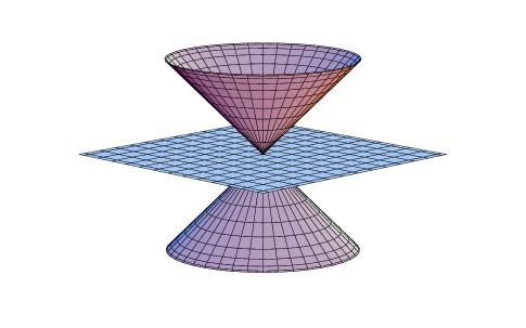
Figure 3.1: A hypersurface in instant form is a hyperplane defining an instant in Minkowski time, here for $x^{0}=t=0$.

From (3.39) and (3.40) we find

$$P^{i}x^{0} = 0,\quad M^{ij}x^{0}=-M^{ji}x^{0}=0,$$ (3.42)

$$P^{0}x^{0} \neq 0,\quad M^{i0}x^{0}=-M^{0i}x^{0}\neq 0\quad\forall\,i,j=1,\ldots 3.$$ (3.43)

Thus the generators for space translations $P^{i}$ and space rotations $J^{i}=\epsilon_{ijk}M^{jk}$ are kinematic. The generator for Minkowskian time evolution $H_{t}=P^{0}$ and the generators for Lorentz boosts $B^{i}=M^{i0}$ become dynamic. Hence, time evolution from $\Sigma_{t}$ to $\Sigma_{t+\Delta t}$ will be generated by $P^{0}$ (cf. Figures 3.2 and 3.3). Furthermore, $\Sigma_{t}$ will be invariant under space translations and rotations, but not boost invariant, which is an expected result since boost mix space and time.

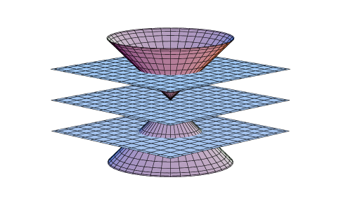
Figure 3.2: Time development in instant form generated by $P^{0}$.

\psfrag{St2}{$\Sigma_{t_{2}}$}\psfrag{St1}{$\Sigma_{t_{1}}$}\psfrag{S0}{$\Sigma_{t_{0}}$}\psfrag{0}{$0$}\psfrag{x0}{$x^{0}$}\psfrag{vecx}{$\boldsymbol{x}$}\includegraphics[clip={100cm},width=227.62204pt]{ifsc.eps}

Figure 3.3: Time development in instant form generated by $P^{0}$ corresponds to evolution from one hyperplane $\Sigma_{t}:x^{0}=t$ to another $\Sigma_{t+\Delta t}:x^{0}=t+\Delta t$ (for $t,\Delta t=\mathrm{const.}$), here illustrated for $t_{0}=0<t_{1}<t_{2}$.

3.2.2 Front Form

The choice $\tau=x^{0}+x^{3}=:x^{+}$ corresponds to a hypersurface $\Sigma_{x^{+}}$ representing a hyperplane tangent to the light cone, the, so called, null plane (cf. Figure 3.4). In front form it is useful to introduce light-cone coordinates with a metric tensor containing off-diagonal elements. Furthermore, $n^{\mu}$ from (3.18) does not coincide with $\dot{x}^{\mu}$ from (3.19), but $n_{\mu}\dot{x}^{\mu}=1$ still holds. At this point we won’t go into details, but just to mention the important feature of the front form having the largest stability group with dimension 7.

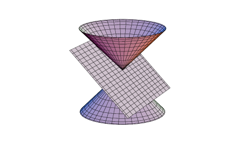
Figure 3.4: The hypersurface in front form is the null plane defining an instant in $x^{-}$.

3.2.3 Point Form

The choice $\xi^{0}\left(x\right)=\tau=\sqrt{x_{\lambda}\,x^{\lambda}}$ of time corresponds to a curved equal-$\tau$ hypersurface $\Sigma_{\tau}:x_{\lambda}\,x^{\lambda}=\tau^{2}$ describing a hyperboloid in space-time (Figure 3.5).

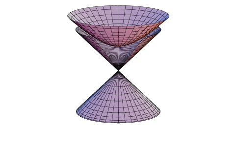
Figure 3.5: A hypersurface in point form is a hyperboloid defining an instant in $\tau$.

The curvilinear coordinates parameterizing these hyperboloids are introduced by the coordinate transformation

$$x^{\mu}\left(\alpha,\beta,\vartheta,\varphi\right)=\mathrm{e}^{\alpha}\left(\begin{array}[]{c}\mathrm{cosh}\beta\\ \mathrm{sinh}\beta\,\mathrm{sin}\vartheta\,\mathrm{cos}\varphi\\ \mathrm{sinh}\beta\,\mathrm{sin}\vartheta\,\mathrm{sin}\varphi\\ \mathrm{sinh}\beta\,\mathrm{cos}\vartheta\end{array}\right)^{\mu},$$ (3.48)

with $\mathrm{e}^{\alpha}=\tau$. The metric is given by

$$\eta_{\mu\nu}\left(\tau,\beta,\vartheta,\varphi\right)=\left(\begin{array}[]{cccc}1&0&0&0\\ 0&-\tau^{2}&0&0\\ 0&0&-\tau^{2}\mathrm{sinh}^{2}\beta&0\\ 0&0&0&-\tau^{2}\mathrm{sinh}^{2}\beta\,\mathrm{sin}^{2}\vartheta\end{array}\right)_{\mu\nu}.$$ (3.53)

This leads together with (3.21) to the world-line metric

$$\eta\left(\tau\right)=1-\tau^{2}\left(\frac{\mathrm{d}\beta}{\mathrm{d}\tau}\right)^{2}-\tau^{2}\mathrm{sinh}^{2}\beta\left(\frac{\mathrm{d}\vartheta}{\mathrm{d}\tau}\right)^{2}-\tau^{2}\mathrm{sinh}^{2}\beta\,\mathrm{sin}^{2}\vartheta\left(\frac{\mathrm{d}\varphi}{\mathrm{d}\tau}\right)^{2}.$$ (3.54)

From (3.18) we find for the normal vector on the hyperboloid $\Sigma_{\tau}$, $n^{\mu}\left(x\right)=\frac{x^{\mu}}{\tau}$. This is in that case identical with the velocity $\frac{\mathrm{d}x^{\mu}}{\mathrm{d}\tau}$ (3.19) and can be interpreted as a four-dimensional radial vector. The Hamiltonian, i.e. the generator for $\tau$-evolution from $\Sigma_{\tau}$ to $\Sigma_{\tau+\Delta\tau}$ is given by (3.37) as

$$H_{\tau}\equiv D=n_{\lambda}\,P^{\lambda}=\frac{x_{\lambda}\,P^{\lambda}}{\tau},\quad\tau\neq 0.$$ (3.55)

$H_{\tau}$ is identified as the generator for dilatation transformations denoted by $D$, which does not belong to the Poincaré group but to the bigger conformal group. From (3.55) we note the explicit $\tau$-dependence. Furthermore, $D$ is only defined for $\tau>0$, thus $\tau$-evolution is restricted to the forward light cone (cf. Figures 3.6 and 3.7). It becomes rather difficult to describe $\tau$-evolution from the backward light cone to the forward light cone, which is necessary when formulating a scattering theory within this approach (cf. Chapter 5).
From (3.39) and (3.40) we find that

$$P^{\mu}\sqrt{x_{\lambda}\,x^{\lambda}}\neq 0,\quad M^{\mu\nu}\sqrt{x_{\lambda}\,x^{\lambda}}=0.$$ (3.56)

This shows that in point form the generators for space-time translations become dynamic, whereas the generators for Lorentz transformations are kinematic. This manifest Lorentz covariance is the typical feature of the point form.

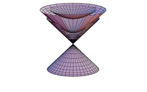
Figure 3.6: $\tau$-development generated by $D$.

\psfrag{St3}{$\Sigma_{\tau_{3}}$}\psfrag{St2}{$\Sigma_{\tau_{2}}$}\psfrag{St1}{$\Sigma_{\tau_{1}}$}\psfrag{St0}{$\Sigma_{\tau_{0}}$}\psfrag{0}{$0$}\psfrag{x0}{$x^{0}$}\psfrag{vecx}{$\boldsymbol{x}$}\includegraphics[clip={7cm},width=227.62204pt]{pfev.eps}

Figure 3.7: $\tau$-development generated by the dilatation generator $D$ corresponds to evolution from one hyperboloid, $\Sigma_{\tau}:x_{\lambda}\,x^{\lambda}=\tau^{2}$ to another $\Sigma_{\tau+\Delta\tau}:x_{\lambda}\,x^{\lambda}=\left(\tau+\Delta\tau\right)^{2}$ (for $\tau,\Delta\tau=\mathrm{const.}$), here illustrated for $\tau_{0}=0<\tau_{1}<\tau_{2}<\tau_{3}$. Note that $\Sigma_{\tau=0}$ represents the light cone.

3.3 General Evolution

From (2.32) and (2.45) we are able to derive a general formula for a Hamiltonian of a system with a given foliation $\tau=\xi^{0}\left(x\right)$ that generates displacements of a hypersurface $\Sigma_{\tau}$. We define the operator $G_{\zeta}$ by means of the energy-momentum tensor (2.31) as

$$G_{\zeta}=\int_{\Sigma}\mathrm{d}\Sigma_{\tau}^{\nu}\left(x\right)\zeta_{\mu}\left(x\right)\mathcal{T}^{\mu}_{\nu}\left(x\right),$$ (3.57)

where

$$\mathrm{d}\Sigma_{\tau}^{\mu}\left(x\right) = \mathrm{d}^{4}x\frac{\partial\xi^{0}\left(x\right)}{\partial x_{\mu}}\delta\left(\xi^{0}\left(x\right)-\tau\right)=\mathrm{d}^{4}x\,n^{\mu}\left(x\right)\delta\left(\xi^{0}\left(x\right)-\tau\right)$$ (3.58)

$$= n^{\mu}\left(x\right)\mathrm{d}\Sigma_{\tau}\left(x\right).$$

The quantity $G_{\zeta}$ generates the infinitesimal transformation

$$x^{\mu}\mapsto x^{\prime\mu}=x^{\mu}+\zeta^{\mu}\left(x\right),\quad\chi^{\prime}\left(x\right)=\chi\left(x\right)+\zeta^{\mu}\left(x\right)\partial_{\mu}\chi\left(x\right),$$ (3.59)

where $\zeta^{\mu}\left(x\right)$ is a function of $x$. If we choose a particular space-time foliation, we find two classes of operators from (3.57), depending on the form of $\zeta^{\mu}\left(x\right)$. The operators of the first class are called kinematic, if the hypersurface $\Sigma_{\tau}:~{}\tau=\xi^{0}\left(x\right)$ is invariant under transformations (3.59), i.e.

$$\delta\xi^{0}\left(x\right):=\xi^{0}\left(x^{\prime}\right)-\xi^{0}\left(x\right)=\zeta^{\mu}\left(x\right)\partial_{\mu}\xi^{0}\left(x\right)=\zeta^{\mu}\left(x\right)n_{\mu}\left(x\right)=0.$$ (3.60)

Otherwise, i.e. if

$$\delta\xi^{0}\left(x\right)=\zeta^{\mu}\left(x\right)n_{\mu}\left(x\right)\neq 0,$$ (3.61)

then $G_{\zeta}$ belongs to the second class and is called dynamic.
When including interactions into the energy-momentum tensor via an interaction Lagrangian $\mathcal{L}_{\mathrm{int}}\left(x\right)$

$$\mathcal{T}^{\mu\nu}\left(x\right)\rightarrow\mathcal{T}^{\mu\nu}\left(x\right)-g^{\mu\nu}\mathcal{L}_{\mathrm{int}}\left(x\right),$$ (3.62)

we find that the kinematic operators are independent of $\mathcal{L}_{\mathrm{int}}$. The interaction part of $G_{\zeta}$ is

$$-\int_{\mathbb{R}^{4}}\mathrm{d}^{4}x\,\delta\left(\xi^{0}\left(x\right)-\tau\right)n^{\mu}\left(x\right)\zeta_{\mu}\left(x\right)\mathcal{L}_{\mathrm{int}}\left(x\right)=0,$$ (3.63)

if (3.60) holds. We note the important result, that when including interactions into the theory, the dynamic operators become interaction dependent, whereas the kinematic operators stay interaction free.
Furthermore, for particular choices of $\zeta^{\mu}\left(x\right)$ we recover the generators of the Poincaré group: $P^{\mu}$ corresponds to $\zeta^{\mu\nu}\left(x\right)=g^{\mu\nu}$ (cf. (2.32)) and $M^{\mu\nu}$ to the choice $\zeta^{\mu\nu\rho}\left(x\right)=x^{\mu}g^{\nu\rho}-x^{\nu}g^{\mu\rho}$ (cf. (2.45)) [4, 25].

Chapter 4 Covariant Canonical Quantization of Free Fields

The common procedure of canonical quantization consists of posing canonical (anti)commutation relations on the field operators at equal Minkowski times $x^{0}=y^{0}=t$. This corresponds to quantization on the hyperplane $\Sigma_{t}$. Adopting Dirac’s nomenclature [1] we shall call it therefore instant-form field quantization. In Chapter 3 we have found the freedom in choosing a space-time foliation of Minkowski space as a characteristic feature of relativistic parameterized systems. Generalizing these ideas to a field theory leads to canonical (anti)commutation relations imposed on an arbitrary spacelike hypersurface. This corresponds to a particular choice of space-time foliation. In his paper Schwinger [3] proposes this way of generalized canonical field quantization without making a particular choice of time. In the following chapter we shall apply this idea to the point form and quantize field theories on the Lorentz-invariant hyperboloid $\Sigma_{\tau}$ by imposing Lorentz-invariant canonical (anti)commutation relations. Therefore we shall speak of point-form quantum field theory. As we have seen, the particular choice of space-time foliation should not play a role for the dynamics of a relativistic theory. This is expressed by the reparameterization invariance of the action (cf. Section 3.1.2). The Lie algebra (2.4) demanding Poincaré invariance of the theory should hold for any form of dynamics. In particular for a free theory, the Poincaré generators should be essentially the same, which can be explicitly shown using a common Fock basis. To see this equivalence, we will make use of the, so called, Wigner basis which consists of simultaneous eigenstates of the three-momentum and spin.

4.1 Complex Klein-Gordon Fields

We consider a free classical complex scalar field theory in ($3+1$)-dimensional Minkowski space-time, with $\phi\left(x\right),\phi^{\ast}\left(x\right)$ describing fields with electric charge. Starting with a free Klein-Gordon Lagrangian density

$$\mathcal{L}_{\mathrm{KG}}\left(x\right)=\partial_{\mu}\phi^{\ast}\left(x\right)\partial^{\mu}\phi\left(x\right)-m^{2}\phi^{\ast}\left(x\right)\phi\left(x\right),$$ (4.1)

the classical action functional is defined by (2.13)

$$S_{\mathrm{KG}}\left[\phi,\phi^{\ast}\right]:=\int_{\mathbb{R}^{4}}\mathrm{d}^{4}x\,\mathcal{L}_{\mathrm{KG}}\left(x\right).$$ (4.2)

The least action principle (2.14) of varying the action functional with respect to $\phi\left(x\right),\phi^{\ast}\left(x\right)$ gives

$$\frac{\delta S_{\mathrm{KG}}\left[\phi,\phi^{\ast}\right]}{\delta\phi\left(x\right)}\stackrel{{\scriptstyle!}}{{=}}0,\quad\frac{\delta S_{\mathrm{KG}}\left[\phi,\phi^{\ast}\right]}{\delta\phi^{\ast}\left(x\right)}\stackrel{{\scriptstyle!}}{{=}}0.$$ (4.3)

This is equivalent to the Euler-Lagrange equations

$$\frac{\partial\mathcal{L}_{\mathrm{KG}}\left(x\right)}{\partial\phi\left(x\right)}=\partial_{\mu}\frac{\partial\mathcal{L}_{\mathrm{KG}}\left(x\right)}{\partial\left(\partial_{\mu}\phi\left(x\right)\right)},\quad\frac{\partial\mathcal{L}_{\mathrm{KG}}\left(x\right)}{\partial\phi^{\ast}\left(x\right)}=\partial_{\mu}\frac{\partial\mathcal{L}_{\mathrm{KG}}\left(x\right)}{\partial\left(\partial_{\mu}\phi^{\ast}\left(x\right)\right)}.$$ (4.4)

For the Lagrangian density (4.1) these equations of motion are the Klein-Gordon equations

$$\left(\square+m^{2}\right)\phi\left(x\right)=0,\quad\left(\square+m^{2}\right)\phi^{\ast}\left(x\right)=0.$$ (4.5)

4.1.1 Invariant Scalar Product

Let $\phi,\chi$ be arbitrary solutions of the Klein-Gordon equation (4.5). Their inner product can be defined by

$$\left(\phi,\chi\right)_{\Sigma} := i\int_{\Sigma}\mathrm{d}\Sigma^{\mu}\left(x\right)\left[\phi^{\ast}\left(x\right)\left(\partial_{\mu}\chi\left(x\right)\right)-\left(\partial_{\mu}\phi^{\ast}\left(x\right)\right)\chi\left(x\right)\right]$$ (4.6)

$$\equiv i\int_{\Sigma}\mathrm{d}\Sigma^{\mu}\left(x\right)\phi^{\ast}\left(x\right)\overleftrightarrow{\partial_{\mu}}\chi\left(x\right),$$

with $\Sigma$ denoting a spacelike hypersurface of Minkowski space. It can be shown that the inner product (4.6) does not depend on the particular choice of $\Sigma$ [26].
$\circ\quad$ We make use of Gauss’ theorem

$$\int_{\partial\mathcal{U}}\mathrm{d}\Sigma_{\mu}\zeta^{\mu}=\int_{\mathcal{U}}\mathrm{d}^{4}x\,\partial_{\mu}\,\zeta^{\mu},$$ (4.7)

with $\mathcal{U}$ being a compact four-dimensional submanifold of Minkowski space and $\zeta$ a vector field. Let $\Sigma_{1},\Sigma_{2}$ be two different, spacelike hypersurfaces and let $\mathcal{U}$ be bounded by $\Sigma_{1},\Sigma_{2}$ and by suitable timelike hypersurfaces where $\phi=\chi=0$. Then we can write

$$\left(\phi,\chi\right)_{\Sigma_{1}}-\left(\phi,\chi\right)_{\Sigma_{2}} = i\int_{\partial\mathcal{U}}\mathrm{d}\Sigma^{\mu}\left[\phi^{\ast}\left(x\right)\left(\partial_{\mu}\chi\left(x\right)\right)-\left(\partial_{\mu}\phi^{\ast}\left(x\right)\right)\chi\left(x\right)\right]$$ (4.8)

$$= i\int_{\mathcal{U}}\mathrm{d}^{4}x\,\partial^{\mu}\left[\phi^{\ast}\left(x\right)\left(\partial_{\mu}\chi\left(x\right)\right)-\left(\partial_{\mu}\phi^{\ast}\left(x\right)\right)\chi\left(x\right)\right]$$

$$= i\int_{\mathcal{U}}\mathrm{d}^{4}x\left[\phi^{\ast}\left(x\right)\left(\square\,\chi\left(x\right)\right)-\left(\square\,\phi^{\ast}\left(x\right)\right)\chi\left(x\right)\right]$$

$$= i\int_{\mathcal{U}}\mathrm{d}^{4}x\left[m^{2}-m^{2}\right]\phi^{\ast}\left(x\right)\chi\left(x\right)=0,$$

where we have used in the last step that $\phi,\chi$ solve the Klein-Gordon equation (4.5) [26].$\quad\bullet$
We see that it is essential for the inner product to be independent of the hypersurface, that $\phi$ and $\chi$ are solutions of the Klein-Gordon equation. From (3.58) we can write the hypersurface element as

$$\mathrm{d}\Sigma^{\mu}\left(x\right)=n^{\mu}\left(x\right)\mathrm{d}\Sigma\left(x\right).$$ (4.9)

For a hypersurface $\Sigma_{t}$ with fixed Minkowski time $x^{0}=t=\mathrm{const.}$ (cf. Section 3.2.1), we have $\mathrm{d}x^{0}=0$. Therefore, we have for the hypersurface element

$$\mathrm{d}\Sigma_{t}^{\mu}\left(x\right) = \left(\begin{array}[]{c}\mathrm{d}x^{1}\mathrm{d}x^{2}\mathrm{d}x^{3}\\ 0\\ 0\\ 0\\ \end{array}\right)^{\mu}=\left(\begin{array}[]{c}1\\ 0\\ 0\\ 0\\ \end{array}\right)^{\mu}\mathrm{d}^{3}x=g^{0\mu}\mathrm{d}^{3}x.$$ (4.18)

This inserted into (4.6) yields the well known scalar product

$$\left(\phi,\chi\right)_{\Sigma_{t}}:=i\int_{\mathbb{R}^{3}}\mathrm{d}^{3}x\,\phi^{\ast}\left(x\right)\overleftrightarrow{\partial_{0}}\left.\chi\left(x\right)\right|_{x^{0}=t},$$ (4.19)

which is independent of $t$. We shall call (4.19) instant-form scalar product.
Every solution of the Klein-Gordon equation (4.5) can be expanded in terms of plane waves. This means that the functions

$$\phi_{\boldsymbol{p}}\left(x\right)=\frac{1}{\left(2\pi\right)^{\frac{3}{2}}}\mathrm{e}^{-ip_{\lambda}\,x^{\lambda}}\quad\text{and}\quad\phi_{\boldsymbol{p}}^{\ast}\left(x\right)=\frac{1}{\left(2\pi\right)^{\frac{3}{2}}}\mathrm{e}^{ip_{\lambda}\,x^{\lambda}},$$ (4.20)

with $p_{\lambda}\,p^{\lambda}=m^{2}$ provide a complete set. Since the constraint (3.1) holds for (4.20), the solutions of (4.5) can be given a particle interpretation. The modes $\phi_{\boldsymbol{p}}\left(x\right)$ are said to be positive energy and $\phi_{\boldsymbol{p}}^{\ast}\left(x\right)$ negative energy solutions. The scalar product between these modes is

$$\left(\phi_{\boldsymbol{p}},\phi_{\boldsymbol{q}}\right)_{\Sigma_{t}}=2p^{0}\delta^{3}\left(\boldsymbol{p}-\boldsymbol{q}\right),\quad\left(\phi_{\boldsymbol{p}}^{\ast},\phi_{\boldsymbol{q}}^{\ast}\right)_{\Sigma_{t}}=-2p^{0}\delta^{3}\left(\boldsymbol{p}-\boldsymbol{q}\right),$$ (4.21)

$$\left(\phi_{\boldsymbol{p}}^{\ast},\phi_{\boldsymbol{q}}\right)_{\Sigma_{t}}=\left(\phi_{\boldsymbol{p}},\phi_{\boldsymbol{q}}^{\ast}\right)_{\Sigma_{t}}=0.$$ (4.22)

For the hypersurface $\Sigma_{\tau}$ of Section 3.2.3 with fixed $x_{\lambda}\,x^{\lambda}=\tau^{2}=\mathrm{const.}$, we have for the hypersurface element

$$\mathrm{d}\Sigma_{\tau}^{\mu}\left(x\right)=2\,\mathrm{d}^{4}x\delta\left(x_{\lambda}\,x^{\lambda}-\tau^{2}\right)\theta\left(x^{0}\right)x^{\mu}.$$ (4.23)

This is explicitly shown in Appendix A. The inner product over the hyperboloid is given by

$$\left(\phi,\chi\right)_{\Sigma_{\tau}} := i\int_{\mathbb{R}^{4}}2\,\mathrm{d}^{4}x\,\delta\left(x_{\lambda}\,x^{\lambda}-\tau^{2}\right)\theta\left(x^{0}\right)x^{\mu}$$ (4.24)

$$\times\phi^{\ast}\left(x\right)\overleftrightarrow{\partial_{\mu}}\chi\left(x\right).$$

We have to show that the statement (4.8) is true. This means that this scalar product is independent of the chosen hyperboloid characterized by $\tau$. Again using plane waves (4.20) for $\phi,\chi$ the scalar product reads

$$\left(\phi_{\boldsymbol{p}},\phi_{\boldsymbol{q}}\right)_{\Sigma_{\tau}} = \frac{2}{\left(2\pi\right)^{3}}\int_{\mathbb{R}^{4}}\mathrm{d}^{4}x\,\delta\left(x_{\lambda}\,x^{\lambda}-\tau^{2}\right)\theta\left(x^{0}\right)x^{\mu}\left(p+q\right)_{\mu}\mathrm{e}^{ix^{\nu}\left(p-q\right)_{\nu}}$$ (4.25)

$$=: W\left(p+q,p-q\right).$$

This Lorentz-invariant distribution is calculated in Appendix (B.1). Its value is $W\left(p+q,p-q\right)=2p^{0}\delta^{3}\left(\boldsymbol{p}-\boldsymbol{q}\right)$. Similarly, we have

$$\left(\phi_{\boldsymbol{p}}^{\ast},\phi_{\boldsymbol{q}}^{\ast}\right)_{\Sigma_{\tau}}=-W\left(p+q,q-p\right)=-2p^{0}\delta^{3}\left(\boldsymbol{p}-\boldsymbol{q}\right).$$ (4.26)

For the orthogonal plane waves we have

$$\left(\phi_{\boldsymbol{p}},\phi_{\boldsymbol{q}}^{\ast}\right)_{\Sigma_{\tau}} = \frac{2}{\left(2\pi\right)^{3}}\int_{\mathbb{R}^{4}}\mathrm{d}^{4}x\,\delta\left(x_{\lambda}\,x^{\lambda}-\tau^{2}\right)\theta\left(x^{0}\right)x^{\mu}\left(p-q\right)_{\mu}\mathrm{e}^{ix^{\nu}\left(p+q\right)_{\nu}}$$ (4.27)

$$= W\left(p-q,p+q\right)=0$$

as calculated in the Appendix (B.1). Similarly we have

$$\left(\phi^{\ast}_{\boldsymbol{p}},\phi_{\boldsymbol{q}}\right)_{\Sigma_{\tau}}=-W\left(p-q,-p-q\right)=0.$$ (4.28)

Comparing these equations with (4.21) and (4.22) we see, that the inner product is indeed independent of the chosen spacelike hypersurface.

4.1.2 Covariant Canonical Commutation Relations

Now we want to perform the canonical quantization of our fields. For this purpose, we replace the classical scalar fields $\phi,\phi^{\ast}$ by field operators $\hat{\phi},\hat{\phi}^{{\dagger}}$. In order to impose quantization conditions on these field operators, Schwinger [3] proposes covariant canonical commutator relations on an arbitrary spacelike hypersurface

$$\int_{\Sigma}\mathrm{d}\Sigma\left(x\right)\left[\hat{\phi}\left(y\right),\hat{\pi}\left(x\right)\right]_{x,y\in\Sigma}=\int_{\Sigma}\mathrm{d}\Sigma\left(x\right)\left[\hat{\phi}^{{\dagger}}\left(y\right),\hat{\pi}^{{\dagger}}\left(x\right)\right]_{x,y\in\Sigma}=i,$$

(4.29)

$$\left[\hat{\phi}\left(x\right),\hat{\phi}\left(y\right)\right]=\left[\hat{\phi}^{{\dagger}}\left(x\right),\hat{\phi}^{{\dagger}}\left(y\right)\right]=\left[\hat{\pi}\left(x\right),\hat{\pi}\left(y\right)\right]=\left[\hat{\pi}^{{\dagger}}\left(x\right),\hat{\pi}^{{\dagger}}\left(y\right)\right]$$

$$=\left[\hat{\phi}\left(x\right),\hat{\pi}^{{\dagger}}\left(y\right)\right]=\left[\hat{\phi}^{{\dagger}}\left(x\right),\hat{\pi}\left(y\right)\right]=0,\quad x,y\in\Sigma.$$ (4.30)

A generalization of these commutation relations to arbitrary $x$ and $y$ is given by

$$\left[\hat{\phi}\left(x\right),\hat{\phi}^{{\dagger}}\left(y\right)\right]=i\Delta\left(x-y\right),$$ (4.31)

$$\left[\hat{\pi}\left(x\right),\hat{\pi}^{{\dagger}}\left(y\right)\right]=i\,n_{\mu}\left(x\right)n_{\nu}\left(y\right)\,\frac{\partial}{\partial x_{\mu}}\,\frac{\partial}{\partial y_{\nu}}\Delta\left(x-y\right),$$ (4.32)

where $\Delta\left(x-y\right)$ is the, so called, Pauli-Jordan function. The field operator $\hat{\pi}$ canonically conjugate to $\hat{\phi}$ is given by

$$\hat{\pi}\left(x\right)=n^{\mu}\left(x\right)\frac{\partial\hat{\mathcal{L}}_{\mathrm{KG}}\left(x\right)}{\partial\left(\partial^{\mu}\hat{\phi}\left(x\right)\right)}=n^{\mu}\left(x\right)\partial_{\mu}\hat{\phi}^{{\dagger}}\left(x\right)=\frac{\partial}{\partial{\xi^{0}}}\hat{\phi}^{{\dagger}}\left(\xi\right).$$

In the last step we have used the transformation properties of $\partial_{\mu}$. Thus $\hat{\pi}$ is just the derivative of $\hat{\phi}^{{\dagger}}$ with respect to some timelike direction $n^{\mu}\left(x\right)$ depending on the choice of space-time foliation. The real distribution $\Delta\left(x-y\right)$ in (4.31) and its second derivative with respect to a chosen time parameter in (4.32) vanish for spacelike $\left(x-y\right)$. They are given by

$$\Delta\left(x-y\right) = \frac{1}{i}\int_{\mathbb{R}^{4}}\frac{\mathrm{d}^{4}p}{\left(2\pi\right)^{3}}\delta\left(p_{\lambda}\,p^{\lambda}-m^{2}\right)\mathrm{e}^{-ip_{\mu}\left(x-y\right)^{\mu}}$$ (4.34)

$$\times\left(\theta\left(p^{0}\right)-\theta\left(-p^{0}\right)\right)$$

and

$$n_{\mu}\left(x\right)n_{\nu}\left(y\right)\,\frac{\partial}{\partial x_{\mu}}\,\frac{\partial}{\partial y_{\nu}}\Delta\left(x-y\right)$$

$$=\frac{1}{i}\int_{\mathbb{R}^{4}}\frac{\mathrm{d}^{4}p}{\left(2\pi\right)^{3}}\delta\left(p_{\lambda}\,p^{\lambda}-m^{2}\right)\,n_{\mu}\left(x\right)\,p^{\mu}\,n_{\nu}\left(y\right)\,p^{\nu}\,\mathrm{e}^{-ip_{\rho}\left(x-y\right)^{\rho}}\left(\theta\left(p^{0}\right)-\theta\left(-p^{0}\right)\right).$$

Since $p$ is timelike and (4.34) and (4.1.2) are Lorentz invariant, we can immediately conclude, that for spacelike $\left(x-y\right)$ it follows that

$$\Delta\left(x-y\right)=n_{\mu}\left(x\right)n_{\nu}\left(y\right)\,\frac{\partial}{\partial x_{\mu}}\,\frac{\partial}{\partial y_{\nu}}\Delta\left(x-y\right)=0.$$ (4.36)

This is a consequence of locality and causality and explicitly proved in Appendix C.1.
Choosing in (4.1.2) the instant-$t$ plane $\Sigma_{t}$ (4.18) we have

$$\int_{\mathbb{R}^{3}}\mathrm{d}^{3}x\left[\hat{\phi}\left(y\right),\partial_{0}\hat{\phi}^{{\dagger}}\left(x\right)\right]_{x^{0}=y^{0}=t}=i.$$ (4.37)

This relation is satisfied, if the commutator is equal

$$\left[\hat{\phi}\left(y\right),\partial_{0}\hat{\phi}^{{\dagger}}\left(x\right)\right]_{x^{0}=y^{0}=t}=i\delta^{3}\left(\boldsymbol{x}-\boldsymbol{y}\right)$$ (4.38)

and we recover the equal-t canonical commutation relations.
If we choose in (4.1.2) the hyperboloid $\Sigma_{\tau}$ (4.23), we have

$$\int_{\mathbb{R}^{4}}2\mathrm{d}^{4}x\,\delta\left(x_{\lambda}\,x^{\lambda}-\tau^{2}\right)\theta\left(x^{0}\right)x^{\mu}\left[\hat{\phi}\left(y\right),\partial_{\mu}\hat{\phi}^{{\dagger}}\left(x\right)\right]_{x^{2}=y^{2}=\tau^{2}}=i,$$ (4.39)

which yields

$$x^{\mu}\left[\hat{\phi}\left(y\right),\partial_{\mu}\hat{\phi}^{{\dagger}}\left(x\right)\right]_{x^{2}=y^{2}=\tau^{2}}=ix^{0}\delta^{3}\left(\boldsymbol{x}-\boldsymbol{y}\right).$$ (4.40)

These are the Lorentz-invariant canonical commutation relations when quantizing on a hyperboloid. The Lorentz invariance is explicitly seen by noting that the right hand side of (4.40) is the $W$ distribution (cf. Appendix B.1),

$$x^{0}\delta^{3}\left(\boldsymbol{x}-\boldsymbol{y}\right)=\frac{1}{2}W\left(x+y,x-y\right),$$ (4.41)

which is Lorentz invariant by definition.
The commutation relations are covariant in the sense that no particular choice of a Minkowski time parameter has been made.
This result agrees with those of [6] as shown in Appendix C.2. Furthermore we note that differentiation of (4.31) with respect to Minkowski time $x_{0}$ gives [27]

$$\frac{\partial}{\partial y^{0}}\Delta\left(x-y\right)|_{x^{0}=y^{0}=t}=\delta^{3}\left(\boldsymbol{x}-\boldsymbol{y}\right).$$ (4.42)

This is nothing but the instant-form canonical commutation relation (4.38).
The point-form analogue can be formulated as differentiation of (4.31) with respect to $\xi^{0}\left(x\right)=\tau$ using $\tau\frac{\partial}{\partial{\tau}}=y^{\lambda}\frac{\partial}{\partial y^{\lambda}}$, i.e.

$$y^{\lambda}\frac{\partial}{\partial y^{\lambda}}\Delta\left(x-y\right)|_{x^{2}=y^{2}=\tau^{2}}=x^{0}\delta^{3}\left(\boldsymbol{x}-\boldsymbol{y}\right).$$ (4.43)

This is exactly the Lorentz-invariant commutation relation (4.40) we expected.

4.1.3 Commutation Relations in Momentum Space

The general solutions $\phi$ and $\phi^{{\dagger}}$ of the Klein-Gordon equations (4.5) can be written as an expansion in terms of a complete set of solutions. As shown before, usual plane waves (4.20) are orthogonal with respect to the invariant scalar product (4.6). Thus they provide an appropriate basis. Expansion in terms of plane waves is equivalent with a Fourier expansion. Therefore canonical quantization is done by considering the Fourier coefficients as field operators acting on a momentum Fock space (cf. Section 2.2.4). Then the field operators can be written as

$$\hat{\phi}\left(x\right) = \int_{\mathbb{R}^{4}}\mathrm{d}^{4}p\,\delta\left(p_{\lambda}\,p^{\lambda}-m^{2}\right)\theta\left(p^{0}\right)\left(\phi_{\boldsymbol{p}}\,\hat{a}\left(\boldsymbol{p}\right)+\phi_{\boldsymbol{p}}^{\ast}\,\hat{b}^{{\dagger}}\left(\boldsymbol{p}\right)\right)$$ (4.44)

$$= \frac{1}{\left(2\pi\right)^{\frac{3}{2}}}\int_{\mathbb{R}^{3}}\frac{\mathrm{d}^{3}p}{2p_{0}}\left(\mathrm{e}^{-ip_{\mu}x^{\mu}}\hat{a}\left(\boldsymbol{p}\right)+\mathrm{e}^{ip_{\mu}x^{\mu}}\hat{b}^{{\dagger}}\left(\boldsymbol{p}\right)\right),$$

$$\hat{\phi}^{{\dagger}}\left(x\right) = \int_{\mathbb{R}^{4}}\mathrm{d}^{4}p\,\delta\left(p_{\lambda}\,p^{\lambda}-m^{2}\right)\theta\left(p^{0}\right)\left(\phi_{\boldsymbol{p}}^{\ast}\,\hat{a}^{{\dagger}}\left(\boldsymbol{p}\right)+\phi_{\boldsymbol{p}}\,\hat{b}\left(\boldsymbol{p}\right)\right)$$ (4.45)

$$= \frac{1}{\left(2\pi\right)^{\frac{3}{2}}}\int_{\mathbb{R}^{3}}\frac{\mathrm{d}^{3}p}{2p_{0}}\left(\mathrm{e}^{ip_{\mu}x^{\mu}}\hat{a}^{{\dagger}}\left(\boldsymbol{p}\right)+\mathrm{e}^{-ip_{\mu}x^{\mu}}\hat{b}\left(\boldsymbol{p}\right)\right).$$

The phase space measure for massive particles

$$\mathrm{d}^{4}p\,\delta\left(p_{\lambda}\,p^{\lambda}-m^{2}\right)\theta\left(p^{0}\right)=\frac{\mathrm{d}^{3}p}{2p_{0}}$$ (4.46)

is clearly Lorentz invariant with $p^{0}=\sqrt{\boldsymbol{p}^{2}+m^{2}}>0$. The Fourier coefficients $a,b$ being operators after canonical quantization are given by

$$\hat{a}\left(\boldsymbol{p}\right)=\left(\phi_{\boldsymbol{p}},\hat{\phi}\right)_{\Sigma},\quad\hat{a}^{{\dagger}}\left(\boldsymbol{p}\right)=\left(\hat{\phi},\phi_{\boldsymbol{p}}\right)_{\Sigma},$$ (4.48)

$$\hat{b}\left(\boldsymbol{p}\right)=-\left(\hat{\phi},\phi_{\boldsymbol{p}}^{\ast}\right)_{\Sigma},\quad\hat{b}^{{\dagger}}\left(\boldsymbol{p}\right)=-\left(\phi_{\boldsymbol{p}}^{\ast},\hat{\phi}\right)_{\Sigma}.$$

These relations together with the canonical commutation relations (4.1.2) and (4.30) imply the harmonic-oscillator commutation relations

$$\left[\hat{a}\left(\boldsymbol{p}\right),\hat{a}^{{\dagger}}\left(\boldsymbol{q}\right)\right]=\left[\hat{b}\left(\boldsymbol{p}\right),\hat{b}^{{\dagger}}\left(\boldsymbol{q}\right)\right]=2p^{0}\delta^{3}\left(\boldsymbol{p}-\boldsymbol{q}\right),$$ (4.49)

$$\left[\hat{a}\left(\boldsymbol{p}\right),\hat{a}\left(\boldsymbol{q}\right)\right]=\left[\hat{b}\left(\boldsymbol{p}\right),\hat{b}\left(\boldsymbol{q}\right)\right]=\left[\hat{a}\left(\boldsymbol{p}\right),\hat{b}\left(\boldsymbol{q}\right)\right]=\left[\hat{a}\left(\boldsymbol{p}\right),\hat{b}^{{\dagger}}\left(\boldsymbol{q}\right)\right]=0.$$ (4.50)

In Appendix (C.3) this is explicitly shown in point form. These commutation relations in momentum space are the Fourier transforms of (4.1.2) and (4.30). Since the operators $\hat{a}\left(\boldsymbol{p}\right),\hat{b}\left(\boldsymbol{p}\right),\hat{a}^{{\dagger}}\left(\boldsymbol{p}\right)$ and $\hat{b}^{{\dagger}}\left(\boldsymbol{p}\right)$ satisfy the commutation relations (4.49) and (4.50), they may be interpreted as annihilation or creation operators. By acting on a Fock space constructed out of one-particle Hilbert spaces (cf. Section 2.2.4), they annihilate or create field quanta characterized by the continuous three-momentum vector $\boldsymbol{p}$. The mass-shell constraint (3.1) holds, of course. These basis elements of the, so called, Wigner basis are eigenstates of the three-momentum operator $\hat{\boldsymbol{P}}$.
We shall note that the field expansions (4.44) and (4.45) together with the commutation relations (4.49) and (4.50) imply the explicit form of the Pauli-Jordan function $\Delta\left(x-y\right)$ in (4.34).

4.1.4 Generators in Wigner Representation

In order to show the equivalence between equal-$t$ and equal-$\tau$ field quantization, we represent the generators of global gauge transformations and the Poincaré generators in the Wigner basis. For free fields they are expected to be the same in instant and point form [25].

Global Gauge Transformations

In Section 2.2.2 we have seen that the invariance of the Lagrangian density under a global $U\left(1\right)$ phase transformation of the fields implies a conserved current (2.2.2). Inserting the Lagrangian density for free scalar fields (4.1) yields after canonical quantization the current operator

$$\hat{\mathcal{J}}_{\mathrm{KG}}^{\mu}\left(x\right)=i:\hat{\phi}^{{\dagger}}\left(x\right)\overleftrightarrow{\partial^{\mu}}\hat{\phi}\left(x\right):,\quad\text{with}\quad\partial_{\mu}\,\hat{\mathcal{J}}_{\mathrm{KG}}^{\mu}\left(x\right)=0.$$ (4.51)

”:…:” denotes the usual normal ordering, i.e. commuting all creation operators to the left of the annihilation operators and dropping the commutators in order to avoid infinite ground state energies. Integration of the current operator as in (2.23) gives a conserved charge or symmetry operator

$$\hat{Q}_{\mathrm{KG}} = \int_{\Sigma}\mathrm{d}\Sigma_{\mu}\left(x\right)\hat{\mathcal{J}}_{\mathrm{KG}}^{\mu}\left(x\right)$$ (4.52)

$$= i\int_{\Sigma}\mathrm{d}\Sigma_{\mu}\left(x\right):\hat{\phi}^{{\dagger}}\left(x\right)\overleftrightarrow{\partial^{\mu}}\hat{\phi}\left(x\right):.$$

Inserting the field expansions (4.44) and (4.45) and choosing the equal-t hyperplane $\Sigma_{t}$ one ends up with the well known form for the charge operator in Wigner representation

$$\hat{Q}_{\mathrm{KG}}=\int_{\mathbb{R}^{3}}\mathrm{d}^{3}x\,\hat{\mathcal{J}}_{\mathrm{KG}}^{0}\left(x\right)=\int_{\mathbb{R}^{3}}\frac{\mathrm{d}^{3}p}{2p_{0}}\left(\hat{a}^{{\dagger}}\left(\boldsymbol{p}\right)\hat{a}\left(\boldsymbol{p}\right)-\hat{b}^{{\dagger}}\left(\boldsymbol{p}\right)\hat{b}\left(\boldsymbol{p}\right)\right).$$ (4.53)

This result suggests to consider $\hat{a}^{{\dagger}}\left(\boldsymbol{p}\right)$ and $\hat{a}\left(\boldsymbol{p}\right)$ as creation and annihilation operators of particles with charge $+1$ and $\hat{b}^{{\dagger}}\left(\boldsymbol{p}\right)$ and $\hat{b}\left(\boldsymbol{p}\right)$ as creation and annihilation operators of antiparticles with charge $-1$, respectively.
If we choose the equal-$\tau$ hyperboloid $\Sigma_{\tau}$ as the spacelike hypersurface, we have

$$\hat{Q}_{\mathrm{KG}} = 2i\int_{\mathbb{R}^{4}}\mathrm{d}^{4}x\,\delta\left(x_{\lambda}\,x^{\lambda}-\tau^{2}\right)\theta\left(x^{0}\right)x_{\mu}:\hat{\phi}^{{\dagger}}\left(x\right)\overleftrightarrow{\partial^{\mu}}\hat{\phi}\left(x\right):$$ (4.54)

$$= \int_{\mathbb{R}^{3}}\frac{\mathrm{d}^{3}p}{2p_{0}}\left(\hat{a}^{{\dagger}}\left(\boldsymbol{p}\right)\hat{a}\left(\boldsymbol{p}\right)-\hat{b}^{{\dagger}}\left(\boldsymbol{p}\right)\hat{b}\left(\boldsymbol{p}\right)\right),$$

as calculated in Appendix C.4.1. Comparing (4.53) with (4.54) we see that the charge operator integrated over the hyperboloid has the usual form in Wigner representation.
This result confirms (2.24) on using the canonical commutation relations (4.49) and (4.50), i.e.

$$\hat{\phi}\left(x\right)=\left[\hat{\phi}\left(x\right),\hat{Q}_{\mathrm{KG}}\right].$$ (4.55)

Translations

We have seen in Section 2.2.2 that a conserved current, the energy-momentum tensor (2.31), follows from the invariance of the action under displacements. Inserting for the Lagrangian density (4.1), the energy-momentum tensor becomes after canonical quantization

$$\hat{\mathcal{T}}_{\mathrm{KG}}^{\mu\nu}\left(x\right) = \,:\partial^{\mu}\hat{\phi}^{{\dagger}}\left(x\right)\partial^{\nu}\hat{\phi}\left(x\right)+\partial^{\nu}\hat{\phi}^{{\dagger}}\left(x\right)\partial^{\mu}\hat{\phi}\left(x\right)$$ (4.57)

$$-g^{\mu\nu}\left(\partial_{\lambda}\hat{\phi}^{{\dagger}}\left(x\right)\partial^{\lambda}\hat{\phi}\left(x\right)-m^{2}\hat{\phi}^{{\dagger}}\left(x\right)\hat{\phi}\left(x\right)\right):,$$

$$\text{with}\quad\partial_{\mu}\,\hat{\mathcal{T}}_{\mathrm{KG}}^{\mu\nu}\left(x\right)=0.$$

From equation (3.57) we have obtained the four-momentum operator (2.32) as integral over a spacelike hypersurface. Applying this to (4.57) we have

$$\hat{P}_{\mathrm{KG}}^{\mu}=\int_{\Sigma}\mathrm{d}\Sigma_{\nu}\left(x\right)\hat{\mathcal{T}}_{\mathrm{KG}}^{\mu\nu}\left(x\right).$$ (4.58)

Inserting the field expansions (4.44), (4.45) and taking the equal-$t$ hyperplane $\Sigma_{t}$, we obtain the usual result for the translation generator in Wigner representation

$$\hat{P}_{\mathrm{KG}}^{\mu}=\int_{\mathbb{R}^{3}}\mathrm{d}^{3}x\,\hat{\mathcal{T}}_{\mathrm{KG}}^{\mu 0}\left(x\right)=\int_{\mathbb{R}^{3}}\frac{\mathrm{d}^{3}p}{2p_{0}}p^{\mu}\left(\hat{a}^{{\dagger}}\left(\boldsymbol{p}\right)\hat{a}\left(\boldsymbol{p}\right)+\hat{b}^{{\dagger}}\left(\boldsymbol{p}\right)\hat{b}\left(\boldsymbol{p}\right)\right).$$ (4.59)

Integration over the hyperboloid $\Sigma_{\tau}$ gives, after some calculation (cf. Appendix C.4.2), the same result as in instant form

$$\hat{P}^{\mu}_{\mathrm{KG}} = \int_{\mathbb{R}^{4}}2\mathrm{d}^{4}x\,\delta\left(x_{\lambda}\,x^{\lambda}-\tau^{2}\right)\theta\left(x^{0}\right)x_{\nu}\hat{\mathcal{T}}_{\mathrm{KG}}^{\mu\nu}\left(x\right)$$ (4.60)

$$= \int_{\mathbb{R}^{3}}\frac{\mathrm{d}^{3}p}{2p_{0}}p^{\mu}\left(\hat{a}^{{\dagger}}\left(\boldsymbol{p}\right)\hat{a}\left(\boldsymbol{p}\right)+\hat{b}^{{\dagger}}\left(\boldsymbol{p}\right)\hat{b}\left(\boldsymbol{p}\right)\right).$$

We easily convince ourselves that $\hat{P}_{\mathrm{KG}}^{\mu}$ still transforms as a four-vector under Lorentz transformations:

$$\hat{U}\left(\Lambda\right)\hat{P}^{\mu}_{\mathrm{KG}}\hat{U}\left(\Lambda\right)^{-1} = \int_{\mathbb{R}^{3}}\frac{\mathrm{d}^{3}p}{2p_{0}}p^{\mu}\left(\hat{a}^{{\dagger}}\left(\boldsymbol{\Lambda p}\right)\hat{a}\left(\boldsymbol{\Lambda p}\right)+\hat{b}^{{\dagger}}\left(\boldsymbol{\Lambda p}\right)\hat{b}\left(\boldsymbol{\Lambda p}\right)\right)$$ (4.61)

$$= \int_{\mathbb{R}^{3}}\frac{\mathrm{d}^{3}p}{2p_{0}}\left(\Lambda^{-1}p\right)^{\mu}\left(\hat{a}^{{\dagger}}\left(\boldsymbol{p}\right)\hat{a}\left(\boldsymbol{p}\right)+\hat{b}^{{\dagger}}\left(\boldsymbol{p}\right)\hat{b}\left(\boldsymbol{p}\right)\right)$$

$$= \left(\Lambda^{-1}\right)^{\mu}_{~{}\nu}\hat{P}^{\nu}_{\mathrm{KG}},$$

where $\boldsymbol{\Lambda p}$ means the spatial component of $\Lambda p$. We have used Lorentz invariance of the integration measure and the Lorentz-transformation properties of single-particle states [28]

$$\hat{U}\left(\Lambda\right)\hat{a}^{{\dagger}}\left(\boldsymbol{p}\right)\hat{U}^{-1}\left(\Lambda\right)=\hat{a}^{{\dagger}}\left(\boldsymbol{\Lambda p}\right).$$ (4.62)

This Fock space representation of $\hat{P}_{\mathrm{KG}}^{\mu}$ together with the harmonic-oscillator commutation relations leads to the conclusion, that the field quanta created by $\hat{a}^{{\dagger}}\left(\boldsymbol{p}\right)$ and $\hat{b}^{{\dagger}}\left(\boldsymbol{p}\right)$ are eigenstates of the free four-momentum operator with eigenvalues $p^{\mu}$.
Finally by using the canonical commutation relations (4.49) and (4.50) we confirm (2.33), namely that

$$\partial^{\mu}\hat{\phi}\left(x\right)=i\left[\hat{P}_{\mathrm{KG}}^{\mu},\hat{\phi}\left(x\right)\right].$$ (4.63)

Lorentz Transformations

In Section 2.2.2 we have seen from the invariance of the action under Lorentz transformations, that a conserved current follows, the so called angular-momentum density (2.43). With the energy-momentum tensor (4.57) this gives an operator

$$\hat{\mathcal{M}}_{\mathrm{KG}}^{\mu\nu\sigma}\left(x\right):=x^{\nu}\hat{\mathcal{T}}_{\mathrm{KG}}^{\mu\sigma}\left(x\right)-x^{\sigma}\hat{\mathcal{T}}_{\mathrm{KG}}^{\mu\nu}\left(x\right),\quad\text{with}\quad\partial_{\mu}\,\hat{\mathcal{M}}_{\mathrm{KG}}^{\mu\nu\sigma}\left(x\right)=0.$$ (4.64)

From (3.57) we find the associated conserved charges, the generators for Lorentz transformations as

$$\hat{M}_{\mathrm{KG}}^{\mu\nu}=\int_{\Sigma}\mathrm{d}\Sigma_{\lambda}\left(x\right)\hat{\mathcal{M}}_{\mathrm{KG}}^{\lambda\mu\nu}\left(x\right)=\int_{\Sigma}\mathrm{d}\Sigma_{\lambda}\left(x\right)\left[x^{\mu}\hat{\mathcal{T}}_{\mathrm{KG}}^{\lambda\nu}\left(x\right)-x^{\nu}\hat{\mathcal{T}}_{\mathrm{KG}}^{\lambda\mu}\left(x\right)\right].$$ (4.65)

Inserting for the energy-momentum tensor (4.57) and the field expansions (4.44), (4.45) and integrating over the equal-t hyperplane $\Sigma_{t}$ gives the generators for boosts and rotations in the Wigner representation [15]

$$\hat{M}_{\mathrm{KG}}^{\mu\nu}=\int_{\mathbb{R}^{3}}\frac{\mathrm{d}^{3}p}{2p_{0}}\left(\hat{a}^{{\dagger}}\left(\boldsymbol{p}\right)l^{\mu\nu}\left(\boldsymbol{p}\right)\hat{a}\left(\boldsymbol{p}\right)+\hat{b}^{{\dagger}}\left(\boldsymbol{p}\right)m^{\mu\nu}\left(\boldsymbol{p}\right)\hat{b}\left(\boldsymbol{p}\right)\right).$$ (4.66)

For $\mu,\nu=0,i$ we have the boost generators $\hat{B}_{\mathrm{KG}}^{i}=\hat{M}_{\mathrm{KG}}^{0i}=-\hat{M}_{\mathrm{KG}}^{i0}$, where $l^{0i}=i\frac{\partial}{\partial p_{i}}p^{0}$ and $m^{0i}=ip^{0}\frac{\partial}{\partial p_{i}}$, with $\frac{\partial}{\partial p_{i}}$ acting to the right. For $\mu,\nu=j,k$ we have the generators for spatial rotations $\hat{J}_{\mathrm{KG}}^{i}=\epsilon_{ijk}\hat{M}_{\mathrm{KG}}^{jk}$, where $l^{ij}=m^{ij}=i\left(p^{i}\frac{\partial}{\partial p_{j}}-p^{j}\frac{\partial}{\partial p_{i}}\right)$.
The similar calculation by integrating over the hyperboloid $\Sigma_{\tau}$ is more complicated but leads to the same result as (4.66).
Finally, we calculate (2.46) using the canonical commutation relations (4.49) and (4.50) as

$$\left(x^{\mu}\partial^{\nu}-x^{\nu}\partial^{\mu}\right)\hat{\phi}\left(x\right)=i\left[\hat{\phi}\left(x\right),\hat{M}_{\mathrm{KG}}^{\mu\nu}\right].$$ (4.67)

4.2 Dirac Fields

Considering a free classical spin-$\frac{1}{2}$ field theory in ($3+1$)-dimensional Minkowski space-time, we can proceed in an analogous way as for scalar fields. We start with a Lagrangian density for the four-component spinor fields $\psi\left(x\right),\bar{\psi}\left(x\right)$,

$$\mathcal{L}_{\mathrm{D}}\left(x\right)=\bar{\psi}\left(x\right)\left(i\gamma^{\lambda}\,\partial_{\lambda}-m\right)\psi\left(x\right),\quad\text{with}\quad\bar{\psi}=\psi^{{\dagger}}\gamma^{0},$$ (4.68)

where $\gamma^{\mu}$ are the $4\times 4$ Dirac matrices . The classical action functional is defined by (2.13) as

$$S_{\mathrm{D}}\left[\psi,\bar{\psi}\right]:=\int_{\mathbb{R}^{4}}\mathrm{d}^{4}x\,\mathcal{L}_{\mathrm{D}}\left(x\right).$$ (4.72)

The least action principle (2.14) of varying the action functional with respect to $\psi\left(x\right),\bar{\psi}\left(x\right)$ gives

$$\frac{\delta S_{\mathrm{D}}\left[\psi,\bar{\psi}\right]}{\delta\psi\left(x\right)}\stackrel{{\scriptstyle!}}{{=}}0,\quad\frac{\delta S_{\mathrm{D}}\left[\psi,\bar{\psi}\right]}{\delta\bar{\psi}\left(x\right)}\stackrel{{\scriptstyle!}}{{=}}0.$$ (4.73)

These equations are equivalent to the Euler-Lagrange equations

$$\frac{\partial\mathcal{L}_{\mathrm{D}}\left(x\right)}{\partial\psi\left(x\right)}=\partial_{\mu}\frac{\partial\mathcal{L}_{\mathrm{D}}\left(x\right)}{\partial\left(\partial_{\mu}\psi\left(x\right)\right)},\quad\frac{\partial\mathcal{L}_{\mathrm{D}}\left(x\right)}{\partial\bar{\psi}\left(x\right)}=\partial_{\mu}\frac{\partial\mathcal{L}_{\mathrm{D}}\left(x\right)}{\partial\left(\partial_{\mu}\bar{\psi}\left(x\right)\right)}.$$ (4.74)

For the Lagrangian density (4.68), these equations of motion are the Dirac equations

$$\left(i\gamma^{\lambda}\,\overrightarrow{\partial}_{\lambda}-m\right)\psi\left(x\right) = 0$$ (4.75)

$$\bar{\psi}\left(x\right)\left(i\gamma^{\lambda}\,\overleftarrow{\partial}_{\lambda}+m\right) = 0,$$ (4.76)

with $\bar{\psi}\overleftarrow{\partial}_{\lambda}\,\gamma^{\lambda}\equiv\left(\partial_{\lambda}\,\bar{\psi}\right)\gamma^{\lambda}$.

4.2.1 Invariant Scalar Product

Let $\psi,\chi$ be arbitrary solutions of the Dirac equation (4.75). Then their inner product on a spacelike hypersurface $\Sigma$ can be defined by

$$\left(\psi,\chi\right)_{\Sigma}:=\int_{\Sigma}\mathrm{d}\Sigma^{\mu}\left(x\right)\bar{\psi}\left(x\right)\gamma_{\mu}\chi\left(x\right).$$ (4.77)

Similarly as in Section 4.1.1, (4.77) does not depend on $\Sigma$ [26]. Proceeding in the same way as in Section 4.1.1 this is proved as follows:

$$\circ\quad\left(\psi,\chi\right)_{\Sigma_{1}}-\left(\phi,\chi\right)_{\Sigma_{2}} = \int_{\partial\mathcal{U}}\mathrm{d}\Sigma^{\mu}\left(x\right)\bar{\psi}\left(x\right)\gamma_{\mu}\chi\left(x\right)$$ (4.78)

$$= \int_{\mathcal{U}}\mathrm{d}^{4}x\,\partial^{\mu}\left(\bar{\psi}\left(x\right)\gamma_{\mu}\chi\left(x\right)\right)$$

$$= \int_{\mathcal{U}}\mathrm{d}^{4}x\left[\left(\partial^{\mu}\bar{\psi}\left(x\right)\right)\gamma_{\mu}\chi\left(x\right)+\bar{\psi}\left(x\right)\gamma_{\mu}\left(\partial^{\mu}\chi\left(x\right)\right)\right]$$

$$= i\int_{\mathcal{U}}\mathrm{d}^{4}x\left[m-m\right]\bar{\psi}\left(x\right)\chi\left(x\right)=0,$$

where we have used in the last step that $\bar{\psi},\chi$ solve the Dirac equations (4.75) and (4.76), respectively.$\quad\bullet$
The equal-$t$ hyperplane $\Sigma_{t}$ yields the usual instant-form scalar product

$$\left(\psi,\chi\right)_{\Sigma_{t}}=\int_{\mathbb{R}^{3}}\mathrm{d}^{3}x\,\bar{\psi}\left(x\right)\gamma_{0}\,\chi\left(x\right)=\int_{\mathbb{R}^{3}}\mathrm{d}^{3}x\,\psi^{{\dagger}}\left(x\right)\chi\left(x\right).$$ (4.79)

Every solution of the Dirac equations (4.75) and (4.76) can be written as an expansion of a set of orthogonal solutions. A complete set is given by the normalized four-spinors

$$\psi_{\rho,\boldsymbol{p}}\left(x\right)=\phi_{\boldsymbol{p}}u_{\rho}\left(\boldsymbol{p}\right)\quad\text{and}\quad\chi_{\rho,\boldsymbol{p}}\left(x\right)=\phi_{\boldsymbol{p}}^{\ast}v_{\rho}\left(\boldsymbol{p}\right),$$ (4.80)

with $\phi_{\boldsymbol{p}}\left(x\right)$ given by (4.20) and $\rho=\pm\frac{1}{2}$ being the spin-projection quantum number. The spinor modes $\psi_{\rho,\boldsymbol{p}}\left(x\right)$ are said to be positive energy and $\chi_{\rho,\boldsymbol{p}}\left(x\right)$ negative energy solutions.
In the following we want to show that these solutions are orthogonal with respect to their scalar product (4.77) and that this scalar product is independent of the chosen hypersurface.
Since $\psi_{\rho,\boldsymbol{p}}\left(x\right)$ and $\chi_{\rho,\boldsymbol{p}}\left(x\right)$ solve the Dirac equation, the four-spinors $u_{\rho}\left(\boldsymbol{p}\right)$ and $v_{\rho}\left(\boldsymbol{p}\right)$ have to satisfy the momentum-space Dirac equations

$$\left(\gamma^{\mu}p_{\mu}-m\right)u_{\rho}\left(\boldsymbol{p}\right) = 0,$$ (4.81)

$$\left(\gamma^{\mu}p_{\mu}+m\right)v_{\rho}\left(\boldsymbol{p}\right) = 0.$$ (4.82)

The adjoint four-spinors $\bar{u}_{\rho}\left(\boldsymbol{p}\right)$ and $\bar{v}_{\rho}\left(\boldsymbol{p}\right)$ satisfy the adjoint equations

$$\bar{u}_{\rho}\left(\boldsymbol{p}\right)\left(\gamma^{\mu}p_{\mu}-m\right) = 0,$$ (4.83)

$$\bar{v}_{\rho}\left(\boldsymbol{p}\right)\left(\gamma^{\mu}p_{\mu}+m\right) = 0.$$ (4.84)

They can be written in terms of orthogonal two-component spinors $\varsigma_{\rho},\boldsymbol{\varepsilon}\varsigma_{\rho}$ as

$$u_{\rho}\left(\boldsymbol{p}\right) = \sqrt{p^{0}+m}\left(\begin{array}[]{c}\varsigma_{\rho}\\ \frac{\boldsymbol{\sigma}\cdot\boldsymbol{p}}{p^{0}+m}\varsigma_{\rho}\end{array}\right),$$ (4.87)

$$v_{\rho}\left(\boldsymbol{p}\right) = -\sqrt{p^{0}+m}\left(\begin{array}[]{c}\frac{\boldsymbol{\sigma}\cdot\boldsymbol{p}}{p^{0}+m}\boldsymbol{\varepsilon}\varsigma_{\rho}\\ \boldsymbol{\varepsilon}\varsigma_{\rho}\end{array}\right),$$ (4.90)

with

$$\varsigma_{\rho} = \left(\begin{array}[]{c}\frac{1}{2}+\rho\\ \frac{1}{2}-\rho\end{array}\right),\quad\boldsymbol{\varepsilon}=\left(\begin{array}[]{cc}0&1\\ -1&0\end{array}\right)$$ (4.95)

and $\boldsymbol{\sigma}$ being the Pauli matrices. Since $\varsigma_{\rho}^{{\dagger}}\varsigma_{\sigma}=\delta_{\rho\sigma}$ with $\rho,~{}\sigma=\pm\frac{1}{2}$ and $\varsigma_{\rho}^{{\dagger}}\boldsymbol{\varepsilon}\varsigma_{\rho}=0$, we have, using (4.99)

$$\bar{u}_{\rho}\left(\boldsymbol{p}\right)u_{\sigma}\left(\boldsymbol{p}\right)=-\bar{v}_{\rho}\left(\boldsymbol{p}\right)v_{\sigma}\left(\boldsymbol{p}\right)=2m\delta_{\rho\sigma},$$ (4.100)

$$\bar{u}_{\rho}\left(\boldsymbol{p}\right)v_{\sigma}\left(\boldsymbol{p}\right)=\bar{v}_{\rho}\left(\boldsymbol{p}\right)u_{\sigma}\left(\boldsymbol{p}\right)=0,$$ (4.101)

$$u_{\rho}^{{\dagger}}\left(\boldsymbol{p}\right)v_{\sigma}\left(-\boldsymbol{p}\right)=v_{\rho}^{{\dagger}}\left(\boldsymbol{p}\right)u_{\sigma}\left(-\boldsymbol{p}\right)=0.$$

To proceed we use

$$\bar{u}_{\rho}\left(\boldsymbol{p}\right)\gamma^{\mu}u_{\sigma}\left(\boldsymbol{p}\right)=\bar{v}_{\rho}\left(\boldsymbol{p}\right)\gamma^{\mu}v_{\sigma}\left(\boldsymbol{p}\right)=2p^{\mu}\delta_{\rho\sigma}.$$ (4.103)

The instant-form scalar product between the solutions $\psi_{\rho,\boldsymbol{p}}\left(x\right)$ and $\chi_{\rho,\boldsymbol{p}}\left(x\right)$ can now be calculated as

$$\left(\psi_{\rho,\boldsymbol{p}},\psi_{\sigma,\boldsymbol{q}}\right)_{\Sigma_{t}}=2p^{0}\delta_{\rho\sigma}\delta^{3}\left(\boldsymbol{p}-\boldsymbol{q}\right),\quad\left(\chi_{\rho,\boldsymbol{p}},\chi_{\sigma,\boldsymbol{q}}\right)_{\Sigma_{t}}=2p^{0}\delta_{\rho\sigma}\delta^{3}\left(\boldsymbol{p}-\boldsymbol{q}\right),$$ (4.104)

$$\left(\psi_{\rho,\boldsymbol{p}},\chi_{\sigma,\boldsymbol{q}}\right)_{\Sigma_{t}}=\left(\chi_{\rho,\boldsymbol{p}},\psi_{\sigma,\boldsymbol{q}}\right)_{\Sigma_{t}}=0.$$ (4.105)

The modes are orthogonal and the scalar product independent of $t$. Thus, the scalar product between the modes should always give the results of (4.104) and (4.105), independent of the chosen spacelike hypersurface $\Sigma$. The scalar product over the hyperboloid $\Sigma_{\tau}$ with fixed $x_{\lambda}\,x^{\lambda}=\tau^{2}=\mathrm{const.}$ reads

$$\left(\psi,\chi\right)_{\Sigma_{\tau}}:=\int_{\mathbb{R}^{4}}2\mathrm{d}^{4}x\,\delta\left(x_{\lambda}\,x^{\lambda}-\tau^{2}\right)\theta\left(x^{0}\right)x^{\mu}\bar{\psi}\left(x\right)\gamma_{\mu}\chi\left(x\right).$$ (4.106)

Indeed we obtain the same result as above, namely

$$\left(\psi_{\rho,\boldsymbol{p}},\psi_{\sigma,\boldsymbol{q}}\right)_{\Sigma_{\tau}}=2p^{0}\delta_{\rho\sigma}\delta^{3}\left(\boldsymbol{p}-\boldsymbol{q}\right),\quad\left(\chi_{\rho,\boldsymbol{p}},\chi_{\sigma,\boldsymbol{q}}\right)_{\Sigma_{\tau}}=2p^{0}\delta_{\rho\sigma}\delta^{3}\left(\boldsymbol{p}-\boldsymbol{q}\right),$$ (4.107)

$$\left(\psi_{\rho,\boldsymbol{p}},\chi_{\sigma,\boldsymbol{q}}\right)_{\Sigma_{\tau}}=\left(\chi_{\rho,\boldsymbol{p}},\psi_{\sigma,\boldsymbol{q}}\right)_{\Sigma_{\tau}}=0,$$ (4.108)

as shown in Appendix D.1. Thus the inner product is independent of the chosen spacelike hypersurface and (4.78) holds.

4.2.2 Covariant Canonical Anticommutation Relations

Canonical quantization is equivalent to considering the classical fields $\psi,\bar{\psi}$ as field operators $\hat{\psi},\hat{\bar{\psi}}$. As in the scalar case (cf. Section 4.1.2), we can formulate covariant canonical anticommutation relations over a spacelike hypersurface given by[3]

$$\int_{\Sigma}\mathrm{d}\Sigma\left(x\right)\left\{\hat{\psi}_{\alpha}\left(y\right),\hat{\varpi}_{\beta}\left(x\right)\right\}_{x,y\in\Sigma}=\int_{\Sigma}\mathrm{d}\Sigma\left(x\right)\left\{\hat{\bar{\psi}}_{\alpha}\left(y\right),\hat{\bar{\varpi}}_{\beta}\left(x\right)\right\}_{x,y\in\Sigma}=i\delta_{\alpha\beta},$$

(4.109)

$$\left\{\hat{\psi}_{\alpha}\left(x\right),\hat{\psi}_{\beta}\left(y\right)\right\}=\left\{\hat{\varpi}_{\alpha}\left(x\right),\hat{\varpi}_{\beta}\left(y\right)\right\}$$

$$=\left\{\hat{\psi}_{\alpha}\left(x\right),\hat{\bar{\varpi}}_{\beta}\left(y\right)\right\}=\left\{\hat{\bar{\psi}}_{\alpha}\left(x\right),\hat{\varpi}_{\beta}\left(y\right)\right\}=0,\quad x,y\in\Sigma.$$ (4.110)

For arbitrary $x$ and $y$ we may again use the Pauli-Jordan function (cf. Section 4.1.2)

$$\left\{\hat{\psi}_{\alpha}\left(x\right),\hat{\bar{\psi}}_{\beta}\left(y\right)\right\}=i\left(i\gamma^{\mu}\,\frac{\partial}{\partial x^{\mu}}+m\right)_{\alpha\beta}\Delta\left(x-y\right),$$ (4.111)

$$\left\{\hat{\varpi}_{\alpha}\left(x\right),\hat{\bar{\varpi}}_{\beta}\left(y\right)\right\}=i\left[n^{\lambda}\left(x\right)\gamma_{\lambda}\right]_{\beta}^{~{}\gamma}\left[n^{\nu}\left(y\right)\gamma_{\nu}\right]_{\alpha}^{~{}\delta}\left(i\gamma^{\mu}\,\frac{\partial}{\partial x^{\mu}}+m\right)_{\gamma\delta}\Delta\left(x-y\right),$$

(4.112)

with $\alpha,~{}\beta,~{}\gamma,~{}\delta=1,\ldots 4$ being the Dirac-spinor indices and $n^{\lambda}\left(x\right)$ the timelike vector depending on the chosen space-time foliation. The field operator $\hat{\varpi}$ canonically conjugate to $\hat{\psi}$ is given by

$$\hat{\varpi}\left(x\right)=n^{\mu}\left(x\right)\frac{\partial\hat{\mathcal{L}}_{\mathrm{D}}\left(x\right)}{\partial\left(\partial^{\mu}\hat{\psi}\left(x\right)\right)}=in^{\mu}\left(x\right)\hat{\bar{\psi}}\gamma_{\mu}\left(x\right)$$ (4.113)

$$\text{and}\quad\hat{\bar{\varpi}}=\gamma^{0}\hat{\varpi}^{{\dagger}}.$$ (4.114)

Choosing the instant-t plane $\Sigma_{t}$ in (4.2.2), we have

$$\int_{\mathbb{R}^{3}}\mathrm{d}^{3}x\left\{\hat{\psi}_{\alpha}\left(y\right),i\left[\hat{\bar{\psi}}\left(x\right)\gamma_{0}\right]_{\beta}\right\}_{x^{0}=y^{0}=t}=i\delta_{\alpha\beta}.$$ (4.115)

Hence, we can immediately conclude that the equal-t canonical anticommutation relations are

$$\left\{\hat{\psi}_{\alpha}\left(y\right),\left[\hat{\bar{\psi}}\left(x\right)\gamma_{0}\right]_{\beta}\right\}_{x^{0}=y^{0}=t}=\left\{\hat{\psi}_{\alpha}\left(y\right),\hat{\psi^{{\dagger}}}_{\beta}\left(x\right)\right\}_{x^{0}=y^{0}=t}=\delta_{\alpha\beta}\delta^{3}\left(\boldsymbol{x}-\boldsymbol{y}\right).$$

If we chose the hyperboloid $\Sigma_{\tau}$ we have

$$2i\int_{\mathbb{R}^{4}}\mathrm{d}^{4}x\,\delta\left(x_{\lambda}\,x^{\lambda}-\tau^{2}\right)\theta\left(x^{0}\right)x^{\mu}\left\{\hat{\psi}_{\alpha}\left(y\right),\left[\hat{\bar{\psi}}\left(x\right)\gamma_{\mu}\right]_{\beta}\right\}_{x^{2}=y^{2}=\tau^{2}}=i\delta_{\alpha\beta}$$

and we can conclude that

$$x^{\mu}\left\{\hat{\psi}_{\alpha}\left(y\right),\left[\hat{\bar{\psi}}\left(x\right)\gamma_{\mu}\right]_{\beta}\right\}_{x^{2}=y^{2}=\tau^{2}}=x^{0}\delta_{\alpha\beta}\delta^{3}\left(\boldsymbol{x}-\boldsymbol{y}\right).$$ (4.118)

Contracting with $\left[x^{\nu}\,\gamma_{\nu}\right]_{\beta\gamma}$ and using (4.71) gives

$$\left\{\hat{\psi}_{\alpha}\left(y\right),\hat{\bar{\psi}}_{\gamma}\left(x\right)\right\}_{x^{2}=y^{2}=\tau^{2}}=\left[x^{\mu}\,\gamma_{\mu}\right]_{\alpha\gamma}\frac{x^{0}}{x_{\lambda}\,x^{\lambda}}\delta^{3}\left(\boldsymbol{x}-\boldsymbol{y}\right).$$ (4.119)

These are the Lorentz-invariant canonical anticommutation relations when quantizing on a hyperboloid. This result agrees with [6] as shown in Appendix D.2.
For spacelike $\left(x-y\right)$ the Pauli-Jordan function $\Delta\left(x-y\right)$ vanishes (cf. (4.36)), thus, when quantizing on a spacelike hypersurface, only the derivative terms remain in (4.111) and (4.112).
For equal Minkowski times $x^{0}=y^{0}=t$ we recover (4.111) as the usual anticommutation relations [27, 29]

$$\left\{\hat{\psi}_{\alpha}\left(x\right),\hat{\bar{\psi}}_{\beta}\left(y\right)\right\}_{x^{0}=y^{0}=t} = -\gamma^{0}_{\alpha\beta}\,\partial_{0}\Delta\left(x-y\right)\left|{}_{x^{0}=y^{0}=t}\right.=\gamma^{0}_{\alpha\beta}\delta^{3}\left(\boldsymbol{x}-\boldsymbol{y}\right).$$

When taking the hyperboloid $x_{\lambda}\,x^{\lambda}=y_{\lambda}\,y^{\lambda}=\tau^{2}$, we obtain for (4.111)

$$\left\{\hat{\psi}_{\alpha}\left(x\right),\hat{\bar{\psi}}_{\beta}\left(y\right)\right\}_{x^{2}=y^{2}=\tau^{2}}$$

$$=-\left[\gamma^{\mu}\,\partial_{\mu}\right]_{\alpha\beta}\Delta\left(x-y\right)\left|{}_{x^{2}=y^{2}=\tau^{2}}\right.$$

$$=\left[\gamma^{\mu}\right]_{\alpha\beta}\int_{\mathbb{R}^{4}}\frac{\mathrm{d}^{4}p}{\left(2\pi\right)^{3}}\delta\left(p_{\lambda}\,p^{\lambda}-m^{2}\right)\theta\left(p^{0}\right)p_{\mu}\left(\mathrm{e}^{-ip_{\nu}\left(x-y\right)^{\nu}}+\mathrm{e}^{ip_{\nu}\left(x-y\right)^{\nu}}\right)\left|{}_{x^{2}=y^{2}=\tau^{2}}\right.$$

$$=\frac{\left[\gamma^{\mu}\,X_{\mu}\right]_{\alpha\beta}}{X_{\lambda}\,X^{\lambda}}W\left(X,Y\right)\left|{}_{x^{2}=y^{2}=\tau^{2}}\right.=\left[\gamma^{\mu}\,x_{\mu}\right]_{\alpha\beta}\frac{x^{0}}{x_{\lambda}\,x^{\lambda}}\delta^{3}\left(\boldsymbol{x}-\boldsymbol{y}\right),$$ (4.121)

where we have used the properties of the $W$ distribution (cf. Appendix B.1). For the other anticommutator (4.112) we obtain

$$\left\{\hat{\varpi}_{\alpha}\left(x\right),\hat{\bar{\varpi}}_{\beta}\left(y\right)\right\}_{x^{2}=y^{2}=\tau^{2}}$$

$$=\left[n_{\rho}\left(x\right)\gamma^{\rho}\right]_{\beta}^{~{}\gamma}\left[n_{\nu}\left(y\right)\left(\gamma^{\nu}\right)\right]_{\alpha}^{~{}\delta}\left[\gamma^{\mu}\,x_{\mu}\right]_{\gamma\delta}\frac{x^{0}}{x_{\lambda}\,x^{\lambda}}\delta^{3}\left(\boldsymbol{x}-\boldsymbol{y}\right)\left|{}_{x^{2}=y^{2}=\tau^{2}}\right.$$

$$=\left[\gamma^{\nu}\,x_{\nu}\right]_{\alpha\beta}\frac{x^{0}}{x_{\lambda}\,x^{\lambda}}\delta^{3}\left(\boldsymbol{x}-\boldsymbol{y}\right),$$ (4.122)

where we have used the unit vector orthogonal on the hyperboloid being $n^{\mu}\left(x\right)=\frac{x^{\mu}}{\sqrt{x_{\lambda}\,x^{\lambda}}}$  (cf. Section 3.2.3). We see that (4.121) and (4.122) are in agreement with (4.119), as was expected.

4.2.3 Anticommutation Relations in Momentum Space

The general solutions $\psi$ and $\bar{\psi}$ of the Dirac equations (4.75) and (4.76) can be written as expansions in terms of a complete set of modes. $\psi_{\rho,\boldsymbol{p}}$ and $\chi_{\rho,\boldsymbol{p}}$ of (4.80) provide an appropriate set, being orthogonal and normalized with respect to the scalar product (4.77). After canonical quantization we have for the field operators

$$\hat{\psi}\left(x\right) = \sum_{\rho=\pm\frac{1}{2}}\int_{\mathbb{R}^{3}}\frac{\mathrm{d}^{3}p}{2p^{0}}\left(\psi_{\rho,\boldsymbol{p}}\left(x\right)\hat{c}_{\rho}\left(\boldsymbol{p}\right)+\chi_{\rho,\boldsymbol{p}}\left(x\right)\hat{d}_{\rho}^{{\dagger}}\left(\boldsymbol{p}\right)\right)$$

$$= \frac{1}{\left(2\pi\right)^{\frac{3}{2}}}\sum_{\rho=\pm\frac{1}{2}}\int_{\mathbb{R}^{3}}\frac{\mathrm{d}^{3}p}{2p^{0}}\left(\mathrm{e}^{-ip_{\lambda}\,x^{\lambda}}u_{\rho}\left(\boldsymbol{p}\right)\hat{c}_{\rho}\left(\boldsymbol{p}\right)+\mathrm{e}^{ip_{\lambda}\,x^{\lambda}}v_{\rho}\left(\boldsymbol{p}\right)\hat{d}^{{\dagger}}_{\rho}\left(\boldsymbol{p}\right)\right),$$

$$\hat{\bar{\psi}}\left(x\right) = \sum_{\rho=\pm\frac{1}{2}}\int_{\mathbb{R}^{3}}\frac{\mathrm{d}^{3}p}{2p^{0}}\left(\bar{\psi}_{\rho,\boldsymbol{p}}\left(x\right)\hat{c}^{{\dagger}}_{\rho}\left(\boldsymbol{p}\right)+\bar{\chi}_{\rho,\boldsymbol{p}}\left(x\right)\hat{d}_{\rho}\left(\boldsymbol{p}\right)\right)$$

$$= \frac{1}{\left(2\pi\right)^{\frac{3}{2}}}\sum_{\rho=\pm\frac{1}{2}}\int_{\mathbb{R}^{3}}\frac{\mathrm{d}^{3}p}{2p^{0}}\left(\mathrm{e}^{ip_{\lambda}\,x^{\lambda}}\bar{u}_{\rho}\left(\boldsymbol{p}\right)\hat{c}^{{\dagger}}_{\rho}\left(\boldsymbol{p}\right)+\mathrm{e}^{-ip_{\lambda}\,x^{\lambda}}\bar{v}_{\rho}\left(\boldsymbol{p}\right)\hat{d}_{\rho}\left(\boldsymbol{p}\right)\right).$$

The operators $\hat{c},\hat{c}^{{\dagger}},\hat{d}$ and $\hat{d}^{{\dagger}}$ are given by the invariant scalar product (4.77) as

$$\hat{c}_{\rho}\left(\boldsymbol{p}\right)=\left(\psi_{\rho,\boldsymbol{p}},\hat{\psi}\right)_{\Sigma},\quad\hat{c}_{\rho}^{{\dagger}}\left(\boldsymbol{p}\right)=\left(\hat{\psi},\psi_{\rho,\boldsymbol{p}}\right)_{\Sigma},$$ (4.125)

$$\hat{d}_{\rho}\left(\boldsymbol{p}\right)=\left(\hat{\psi},\chi_{\rho,\boldsymbol{p}}\right)_{\Sigma},\quad\hat{d}_{\rho}^{{\dagger}}\left(\boldsymbol{p}\right)=\left(\chi_{\rho,\boldsymbol{p}},\hat{\psi}\right)_{\Sigma}.$$ (4.126)

These relations, together with the canonical anticommutation relations (4.2.2) and (4.2.2), imply the harmonic-oscillator anticommutation relations in momentum space

$$\left\{\hat{c}_{\rho}\left(\boldsymbol{p}\right),\hat{c}^{{\dagger}}_{\sigma}\left(\boldsymbol{q}\right)\right\} = \left\{\hat{d}_{\rho}\left(\boldsymbol{p}\right),\hat{d}^{{\dagger}}_{\sigma}\left(\boldsymbol{q}\right)\right\}=2p^{0}\delta_{\rho\sigma}\delta^{3}\left(\boldsymbol{p}-\boldsymbol{q}\right),$$ (4.127)

$$\left\{\hat{c}_{\rho}\left(\boldsymbol{p}\right),\hat{c}_{\sigma}\left(\boldsymbol{q}\right)\right\} = \left\{\hat{c}^{{\dagger}}_{\rho}\left(\boldsymbol{p}\right),\hat{c}^{{\dagger}}_{\sigma}\left(\boldsymbol{q}\right)\right\}=\left\{\hat{d}_{\rho}\left(\boldsymbol{p}\right),\hat{d}_{\sigma}\left(\boldsymbol{q}\right)\right\}=\left\{\hat{d}^{{\dagger}}_{\rho}\left(\boldsymbol{p}\right),\hat{d}^{{\dagger}}_{\sigma}\left(\boldsymbol{q}\right)\right\}$$ (4.128)

$$= \left\{\hat{c}_{\rho}\left(\boldsymbol{p}\right),\hat{d}^{{\dagger}}_{\sigma}\left(\boldsymbol{q}\right)\right\}=\left\{\hat{d}_{\rho}\left(\boldsymbol{p}\right),\hat{c}^{{\dagger}}_{\sigma}\left(\boldsymbol{q}\right)\right\}=0.$$

In Appendix D.3 this statement is explicitly shown in point form.
Due to these anticommutation relations one may interpret these operators as annihilation or creation operators on a Fock space (2.2.4) annihilating or creating field quanta characterized by the continuous three-momentum vector $\boldsymbol{p}$ and the discrete spin-projection quantum number $\rho$. Therefore the basis consists of simultaneous eigenstates of $\hat{\boldsymbol{P}}$ and a spin operator with eigenvalue $\rho$.
Finally, we shall note that the field expansions (4.2.3) and (4.2.3) together with the anticommutation relations in momentum space (4.127) and (4.128) imply the anticommutation relation (4.111) and (4.112) and the explicit form of the Pauli-Jordan function in (4.34). The anticommutator (4.111), using the field expansions (4.2.3) and (4.2.3) and the anticommutation relations (4.127) and (4.128), is explicitly calculated as

$$\left\{\hat{\psi}_{\alpha}\left(x\right),\hat{\bar{\psi}}_{\beta}\left(y\right)\right\}$$

$$=\int_{\mathbb{R}^{3}}\frac{\mathrm{d}^{3}p}{2p^{0}\left(2\pi\right)^{3}}\sum_{\rho=\pm\frac{1}{2}}$$

$$\quad\times\left(\mathrm{e}^{-ip_{\lambda}\left(x-y\right)^{\lambda}}\left[u_{\rho}\right]_{\alpha}\left(\boldsymbol{p}\right)\left[\bar{u}_{\rho}\right]_{\beta}\left(\boldsymbol{p}\right)+\mathrm{e}^{ip_{\lambda}\left(x-y\right)^{\lambda}}\left[v_{\rho}\right]_{\alpha}\left(\boldsymbol{p}\right)\left[\bar{v}_{\rho}\right]_{\beta}\left(\boldsymbol{p}\right)\right)$$

$$=i\left(i\gamma^{\mu}\,\frac{\partial}{\partial x^{\mu}}+m\right)_{\alpha\beta}\Delta\left(x-y\right),$$ (4.129)

where we have used the projectors (D.8) and (D.9).

4.2.4 Generators in Wigner Representation

As in the scalar case (cf. Section 4.1.4) we want to show the equivalence of instant- and point-form quantization by representing the generators of our theory in the Wigner basis (cf. Section 4.2.3). For free fields they can be shown to have the same form.

Global Gauge Transformations

As we have seen in Section 2.2.2, the existence of a conserved symmetry current (2.2.2) follows from the invariance of the Lagrangian density $\mathcal{L}_{\mathrm{D}}$ (4.68) under the action of global $U\left(1\right)$-symmetry group. After canonical quantization and normal ordering this current reads

$$\hat{\mathcal{J}}_{\mathrm{D}}^{\mu}\left(x\right)=\,:\hat{\bar{\psi}}\left(x\right)\gamma^{\mu}\hat{\psi}\left(x\right):,\quad\text{with}\quad\partial_{\mu}\,\hat{\mathcal{J}}_{\mathrm{D}}^{\mu}\left(x\right)=0.$$ (4.130)

This current integrated over a spacelike hypersurface gives a conserved charge or symmetry operator

$$\hat{Q}_{\mathrm{D}}=\int_{\Sigma}\mathrm{d}\Sigma_{\mu}\left(x\right)\hat{\mathcal{J}}_{\mathrm{D}}^{\mu}\left(x\right)=\int_{\Sigma}\mathrm{d}\Sigma_{\mu}\left(x\right):\hat{\bar{\psi}}\left(x\right)\gamma^{\mu}\hat{\psi}\left(x\right):.$$ (4.131)

Inserting the field expansions (4.2.3) and (4.2.3) and choosing the equal-t hyperplane $\Sigma_{t}$ the resulting charge operator in Wigner representation reads

$$\hat{Q}_{\mathrm{D}}=\sum_{\rho=\pm\frac{1}{2}}\int_{\mathbb{R}^{3}}\frac{\mathrm{d}^{3}p}{2p_{0}}\left(\hat{c}_{\rho}^{{\dagger}}\left(\boldsymbol{p}\right)\hat{c}_{\rho}\left(\boldsymbol{p}\right)-\hat{d}_{\rho}^{{\dagger}}\left(\boldsymbol{p}\right)\hat{d}_{\rho}\left(\boldsymbol{p}\right)\right).$$ (4.132)

As in the scalar case this suggests to consider $\hat{c}_{\rho}^{{\dagger}}\left(\boldsymbol{p}\right)$ and $\hat{c}_{\rho}\left(\boldsymbol{p}\right)$ as creation and annihilation operators of particles with charge $+1$ and $\hat{d}_{\rho}^{{\dagger}}\left(\boldsymbol{p}\right)$ and $\hat{d}_{\rho}\left(\boldsymbol{p}\right)$ as creation and annihilation operators of antiparticles with charge $-1$, respectively.
If we choose the equal-$\tau$ hyperboloid $\Sigma_{\tau}$ as the spacelike hypersurface we obtain the same result as above, namely

$$\hat{Q}_{\mathrm{D}} = \int_{\mathbb{R}^{4}}2\mathrm{d}^{4}x\,\delta\left(x_{\lambda}\,x^{\lambda}-\tau^{2}\right)\theta\left(x^{0}\right)x^{\mu}:\hat{\bar{\psi}}\left(x\right)\gamma^{\mu}\hat{\psi}\left(x\right):$$ (4.133)

$$= \sum_{\rho=\pm\frac{1}{2}}\int_{\mathbb{R}^{3}}\frac{\mathrm{d}^{3}p}{2p_{0}}\left(\hat{c}_{\rho}^{{\dagger}}\left(\boldsymbol{p}\right)\hat{c}_{\rho}\left(\boldsymbol{p}\right)-\hat{d}_{\rho}^{{\dagger}}\left(\boldsymbol{p}\right)\hat{d}_{\rho}\left(\boldsymbol{p}\right)\right).$$

This is calculated in Appendix D.4.1.
Finally we confirm (2.24) by using the canonical anticommutation relations (4.127) and (4.128),

$$\hat{\psi}\left(x\right)=\left[\hat{\psi}\left(x\right),\hat{Q}_{\mathrm{D}}\right].$$ (4.134)

Translations

In Section 2.2.2 we have seen, that the energy-momentum tensor (2.31) follows from the invariance of the action under displacements. Inserting (4.68) for the Lagrangian density $\mathcal{L}_{\mathrm{D}}$, the energy-momentum tensor operator for Dirac fields becomes after canonical quantization

$$\hat{\mathcal{T}}_{\mathrm{D}}^{\mu\nu}\left(x\right)=\frac{i}{2}:\left[\hat{\bar{\psi}}\left(x\right)\gamma^{\mu}\left(\partial^{\nu}\hat{\psi}\left(x\right)\right)-\left(\partial^{\nu}\hat{\bar{\psi}}\left(x\right)\right)\gamma^{\mu}\hat{\psi}\left(x\right)\right]:,$$ (4.135)

$$\text{with}\quad\partial_{\mu}\,\hat{\mathcal{T}}_{\mathrm{D}}^{\mu\nu}\left(x\right)=0.$$ (4.136)

From equation (3.57) we obtain the four-momentum operator

$$\hat{P}_{\mathrm{D}}^{\mu}=\int_{\Sigma}\mathrm{d}\Sigma_{\nu}\left(x\right)\hat{\mathcal{T}}_{\mathrm{D}}^{\mu\nu}\left(x\right).$$ (4.137)

Inserting the field expansions (4.2.3), (4.2.3) and taking the equal-$t$ hyperplane $\Sigma_{t}$ we obtain the usual result for the translation generator in Wigner representation,

$$\hat{P}_{\mathrm{D}}^{\mu}=\sum_{\rho=\pm\frac{1}{2}}\int_{\mathbb{R}^{3}}\frac{\mathrm{d}^{3}p}{2p_{0}}p^{\mu}\left(\hat{c}_{\rho}^{{\dagger}}\left(\boldsymbol{p}\right)\hat{c}_{\rho}\left(\boldsymbol{p}\right)+\hat{d}_{\rho}^{{\dagger}}\left(\boldsymbol{p}\right)\hat{d}_{\rho}\left(\boldsymbol{p}\right)\right).$$ (4.138)

As shown in Appendix (D.4.2), integration over the hyperboloid $\Sigma_{\tau}$ gives the same result,

$$\hat{P}_{\mathrm{D}}^{\mu} = \int_{\mathbb{R}^{4}}2\mathrm{d}^{4}x\,\delta\left(x_{\lambda}\,x^{\lambda}-\tau^{2}\right)\theta\left(x^{0}\right)x_{\nu}\hat{\mathcal{T}}_{\mathrm{D}}^{\mu\nu}\left(x\right)$$ (4.139)

$$= \sum_{\rho=\pm\frac{1}{2}}\int_{\mathbb{R}^{3}}\frac{\mathrm{d}^{3}p}{2p_{0}}p^{\mu}\left(\hat{c}_{\rho}^{{\dagger}}\left(\boldsymbol{p}\right)\hat{c}_{\rho}\left(\boldsymbol{p}\right)+\hat{d}_{\rho}^{{\dagger}}\left(\boldsymbol{p}\right)\hat{d}_{\rho}\left(\boldsymbol{p}\right)\right).$$

$\hat{P}_{\mathrm{D}}^{\mu}$, represented in this basis, still transforms as a four-vector under Lorentz transformations,

$$\hat{U}\left(\Lambda\right)\hat{P}^{\mu}_{\mathrm{D}}\hat{U}\left(\Lambda\right)^{-1} = \sum_{\rho,\sigma,\lambda=\pm\frac{1}{2}}\int_{\mathbb{R}^{3}}\frac{\mathrm{d}^{3}p}{2p_{0}}p^{\mu}\left(\hat{c}_{\sigma}^{{\dagger}}\left(\boldsymbol{\Lambda p}\right)\hat{c}_{\lambda}\left(\boldsymbol{\Lambda p}\right)D^{\frac{1}{2}}_{\sigma\rho}\left(R\left(p,\Lambda\right)\right)D^{\frac{1}{2}\ast}_{\lambda\rho}\left(R\left(p,\Lambda\right)\right)\right.$$ (4.140)

$$+\left.\hat{d}_{\sigma}^{{\dagger}}\left(\boldsymbol{\Lambda p}\right)\hat{d}_{\lambda}\left(\boldsymbol{\Lambda p}\right)D^{\frac{1}{2}}_{\sigma\rho}\left(R\left(p,\Lambda\right)\right)D^{\frac{1}{2}\ast}_{\lambda\rho}\left(R\left(p,\Lambda\right)\right)\right)$$

$$= \sum_{\rho,\sigma,\lambda=\pm\frac{1}{2}}\int_{\mathbb{R}^{3}}\frac{\mathrm{d}^{3}p}{2p_{0}}\left(\Lambda^{-1}p\right)^{\mu}$$

$$\times\left(\hat{c}_{\sigma}^{{\dagger}}\left(\boldsymbol{p}\right)\hat{c}_{\lambda}\left(\boldsymbol{p}\right)D^{\frac{1}{2}}_{\sigma\rho}\left(R\left(\Lambda^{-1}p,\Lambda\right)\right)D^{\frac{1}{2}}_{\rho\lambda}\left(R^{-1}\left(\Lambda^{-1}p,\Lambda\right)\right)\right.$$

$$\quad+\left.\hat{d}_{\sigma}^{{\dagger}}\left(\boldsymbol{p}\right)\hat{d}_{\lambda}\left(\boldsymbol{p}\right)D^{\frac{1}{2}}_{\sigma\rho}\left(R\left(\Lambda^{-1}p,\Lambda\right)\right)D^{\frac{1}{2}}_{\rho\lambda}\left(R^{-1}\left(\Lambda^{-1}p,\Lambda\right)\right)\right)$$

$$= \left(\Lambda^{-1}\right)^{\mu}_{~{}\nu}\hat{P}^{\nu}_{\mathrm{D}}.$$

Here, we have used Lorentz invariance of the integration measure and the Lorentz-transformation properties of single-particle states [28]

$$\hat{U}\left(\Lambda\right)\hat{c}_{\rho}^{{\dagger}}\left(\boldsymbol{p}\right)\hat{U}\left(\Lambda\right)^{-1}=\sum_{\sigma\pm\frac{1}{2}}\hat{c}_{\sigma}^{{\dagger}}\left(\boldsymbol{\Lambda p}\right)D^{\frac{1}{2}}_{\sigma\rho}\left(R\left(p,\Lambda\right)\right).$$ (4.141)

The $D^{\frac{1}{2}}_{\sigma\rho}$ are the matrix elements of the Wigner D-functions. $R$ denotes a Wigner rotation given by

$$R\left(p,\Lambda\right)=\Lambda\left(\Lambda\left(\omega\right)v\right)^{-1}\Lambda\left(\omega\right)\Lambda\left(v\right),$$ (4.142)

with $\Lambda\left(\omega\right)$ being a general Lorentz transformation and $\Lambda\left(v=\frac{p}{m}\right)$ a Lorentz boost.
This Fock-space representation of $\hat{P}_{\mathrm{D}}^{\mu}$ together with the harmonic-oscillator anticommutation relations (4.127), (4.128) leads to the conclusion, that the field quanta created by $\hat{c}_{\rho}^{{\dagger}}\left(\boldsymbol{p}\right)$ and $\hat{d}_{\rho}^{{\dagger}}\left(\boldsymbol{p}\right)$ are eigenstates of the free four-momentum operator with eigenvalues $p^{\mu}$.
Finally, on using the canonical commutation relations (4.127) and (4.128), we confirm that

$$\partial^{\mu}\hat{\psi}\left(x\right)=i\left[\hat{P}_{\mathrm{D}}^{\mu},\hat{\psi}\left(x\right)\right].$$ (4.143)

Lorentz Transformations

From Neother’s theorem in Section 2.2.2, we have found a conserved current under the assumption of the invariance of the action under Lorentz transformations. This current is the, so called, angular-momentum density (2.43). After canonical quantization it is given by

$$\hat{\mathcal{M}}_{\mathrm{D}}^{\mu\nu\sigma}\left(x\right):=x^{\nu}\hat{\mathcal{T}}_{\mathrm{D}}^{\mu\sigma}\left(x\right)-x^{\sigma}\hat{\mathcal{T}}_{\mathrm{D}}^{\mu\nu}\left(x\right),\quad\text{with}\quad\partial_{\mu}\,\hat{\mathcal{M}}_{\mathrm{D}}^{\mu\nu\sigma}\left(x\right)=0.$$ (4.144)

Then, the associated conserved charge operator reads

$$\hat{M}_{\mathrm{D}}^{\mu\nu}=\int_{\Sigma}\mathrm{d}\Sigma_{\lambda}\left(x\right)\hat{\mathcal{M}}_{\mathrm{D}}^{\lambda\mu\nu}\left(x\right)=\int_{\Sigma}\mathrm{d}\Sigma_{\lambda}\left(x\right)\left[x^{\mu}\hat{\mathcal{T}}_{\mathrm{D}}^{\lambda\nu}\left(x\right)-x^{\nu}\hat{\mathcal{T}}_{\mathrm{D}}^{\lambda\mu}\left(x\right)\right].$$ (4.145)

Inserting for the energy-momentum tensor (4.135), the field expansions (4.2.3), (4.2.3) and integrating over the equal-t hyperplane $\Sigma_{t}$ gives [15]

$$\hat{M}_{\mathrm{D}}^{\mu\nu} = \sum_{\rho,\sigma=\pm\frac{1}{2}}\int_{\mathbb{R}^{3}}\frac{\mathrm{d}^{3}p}{2p_{0}}\left\{\hat{c}_{\rho}^{{\dagger}}\left(\boldsymbol{p}\right)u^{{\dagger}}_{\rho}\left(\boldsymbol{p}\right)\left[l^{\mu\nu}\left(\boldsymbol{p}\right)+\frac{1}{2}\sigma^{\mu\nu}\right]u_{\sigma}\left(\boldsymbol{p}\right)\hat{c}_{\sigma}\left(\boldsymbol{p}\right)\right.$$ (4.146)

$$+\left.\hat{d}_{\rho}^{{\dagger}}\left(\boldsymbol{p}\right)v^{T}_{\rho}\left(\boldsymbol{p}\right)\left[m^{\mu\nu}\left(\boldsymbol{p}\right)-\frac{1}{2}\left(\sigma^{T}\right)^{\mu\nu}\right]v^{\ast}_{\sigma}\left(\boldsymbol{p}\right)\hat{d}_{\sigma}\left(\boldsymbol{p}\right)\right\},$$

with $l^{\mu\nu}$ and $m^{\mu\nu}$ given in Section 4.1.4. The similar calculation by integrating over the hyperboloid $\Sigma_{\tau}$ is more complicated but leads to the same result as (4.146).
Finally we find, using the canonical anticommutation relations (4.127) and (4.128), that

$$\left[\left(x^{\mu}\partial^{\nu}-x^{\nu}\partial^{\mu}\right)\delta^{\alpha}_{~{}\beta}-\frac{i}{2}\left[\sigma^{\mu\nu}\right]^{\alpha}_{~{}\beta}\right]\hat{\psi}^{\beta}\left(x\right)=i\left[\hat{\psi}^{\alpha}\left(x\right),\hat{M}_{\mathrm{D}}^{\mu\nu}\right].$$ (4.147)

Chapter 5 Covariant Scattering Theory for Interacting Fields

As we have already mentioned, a necessary condition for the formulation of a scattering theory is a time development that covers the whole Minkowski space. We assume that the interaction is local and decreases fast enough at infinity. This ensures that we can define asymptotic states and a S operator that maps between these states of non-interacting particles (cf. Section 2.2.5). Therefore the Hamiltonian (3.55) that generates $\tau$-development from one hyperboloid to another does not seem to be very useful, since it only covers the forward light cone.
Looking for an evolution that covers the whole Minkowski space we make the choice as in [25]. That is, we keep $\tau$ fixed and shift the hyperboloid along a timelike path. The generators for this evolution are the components of the four-momentum operator. It should, however, be noted that this kind of evolution is clearly not perpendicular to the quantization surface. But as we will see, this fact does not play a significant role for the formulation of a scattering theory.

5.1 Poincaré Generators

When including interactions into a free theory, the kinematic generators stay interaction free, whereas the dynamic generators will contain interaction terms (cf. Section 3.3).
In order to include interactions, we add an interaction term to the free Lagrangian density,

$$\hat{\mathcal{L}}\left(x\right)=\hat{\mathcal{L}}_{\mathrm{free}}\left(x\right)+\hat{\mathcal{L}}_{\mathrm{int}}\left(x\right).$$ (5.1)

In (2.31) we saw that, as long as $\mathcal{L}_{\mathrm{int}}$ does not contain derivatives of the fields, we can write the interaction part of the energy-momentum tensor as

$$\hat{\mathcal{T}}_{\mathrm{int}}^{\mu\nu}\left(x\right)=-g^{\mu\nu}:\hat{\mathcal{L}}_{\mathrm{int}}\left(x\right):.$$ (5.2)

Therefore we have from (2.32) for the interacting part of the four-momentum operator

$$\hat{P}^{\mu}_{\mathrm{int}}=\int_{\Sigma}\mathrm{d}\Sigma_{\nu}\left(x\right)\hat{\mathcal{T}}_{\mathrm{int}}^{\nu\mu}\left(x\right)=-\int_{\Sigma}\mathrm{d}\Sigma_{\nu}\left(x\right)g^{\nu\mu}:\hat{\mathcal{L}}_{\mathrm{int}}\left(x\right):.$$ (5.3)

Choosing the equal-t hyperplane $\Sigma_{t}$ we see immediately, that $\hat{\mathcal{L}}_{\mathrm{int}}$ does not enter the three-components of the four-momentum operator, i.e.

$$\hat{P}^{\mu}_{\mathrm{int}}=\int_{\mathbb{R}^{3}}\mathrm{d}^{3}x\,g_{~{}\nu}^{0}g^{\nu\mu}:\hat{\mathcal{L}}_{\mathrm{int}}\left(x\right):=\int_{\mathbb{R}^{3}}\mathrm{d}^{3}x\,g^{0\mu}:\hat{\mathcal{L}}_{\mathrm{int}}\left(x\right):=\left(\begin{array}[]{c}\hat{P}^{0}_{\mathrm{int}}\\ \boldsymbol{0}\end{array}\right)^{\mu}.$$ (5.6)

On the other hand, if we take the interacting part of the Lorentz generator $\hat{M}^{\mu\nu}$ and integrate over $\Sigma_{t}$ we have

$$\hat{M}^{\mu\nu}_{\mathrm{int}} = \int_{\mathbb{R}^{3}}\mathrm{d}^{3}x\,g_{~{}\sigma}^{0}\left(x^{\mu}g^{\sigma\nu}-x^{\nu}g^{\sigma\mu}\right):\hat{\mathcal{L}}_{\mathrm{int}}\left(x\right):$$ (5.7)

$$= \int_{\mathbb{R}^{3}}\mathrm{d}^{3}x\,\left(x^{\mu}g^{0\nu}-x^{\nu}g^{0\mu}\right):\hat{\mathcal{L}}_{\mathrm{int}}\left(x\right):.$$

This expression does not vanish, if either $\mu=k\,\wedge\,\nu=0$ or $\nu=k\,\wedge\,\mu=0$ for $k=1,\ldots 3$, i.e. for boost generators $\hat{B}^{k}=\hat{M}^{0k}=-\hat{M}^{k0}$. Hence, we see explicitly that the boost generators together with $\hat{P}^{0}$ become interaction dependent in instant form, which is exactly the statement in Section 3.3.

In point form we have the equal-$\tau$ hyperboloid $\Sigma_{\tau}$ giving

$$\hat{P}^{\mu}_{\mathrm{int}} = \int_{\mathbb{R}^{4}}2\,\mathrm{d}^{4}x\,\delta\left(x_{\lambda}\,x^{\lambda}-\tau^{2}\right)\theta\left(x^{0}\right)x_{\nu}\hat{\mathcal{T}}_{\mathrm{int}}^{\nu\mu}\left(x\right)$$ (5.8)

$$= -\int_{\mathbb{R}^{4}}2\,\mathrm{d}^{4}x\,\delta\left(x_{\lambda}\,x^{\lambda}-\tau^{2}\right)\theta\left(x^{0}\right)x^{\mu}:\hat{\mathcal{L}}_{\mathrm{int}}\left(x\right):.$$

We see explicitly that all components of the four-momentum operator become interaction dependent. On the other hand, the antisymmetric tensor $\hat{M}^{\mu\nu}$ stays interaction free, i.e. the interaction dependent part of this tensor vanishes

$$\hat{M}^{\mu\nu}_{\mathrm{int}} = 2\int_{\mathbb{R}^{4}}\mathrm{d}^{4}x\,\delta\left(x_{\lambda}\,x^{\lambda}-\tau^{2}\right)\theta\left(x^{0}\right)x_{\sigma}\left(x^{\mu}\hat{\mathcal{T}}_{\mathrm{int}}^{\sigma\nu}\left(x\right)-x^{\nu}\hat{\mathcal{T}}_{\mathrm{int}}^{\sigma\mu}\left(x\right)\right)$$ (5.9)

$$= -2\int_{\mathbb{R}^{4}}\mathrm{d}^{4}x\,\delta\left(x_{\lambda}\,x^{\lambda}-\tau^{2}\right)\theta\left(x^{0}\right)x_{\sigma}\left(x^{\mu}g^{\sigma\nu}-x^{\nu}g^{\sigma\mu}\right):\hat{\mathcal{L}}_{\mathrm{int}}\left(x\right):$$

$$= 0.$$

Again we observe that the statement in Section 3.3 holds.
Finally, it should be noted that quantization on the hyperboloid provides a representation of the Poincaré algebra (2.4) expressed by the, so called, point-form equations [28, 31]

$$\left[\hat{P}^{\mu},\hat{P}^{\nu}\right] = 0,$$ (5.10)

$$\hat{U}\left(\Lambda\right)\hat{P}^{\mu}\hat{U}\left(\Lambda\right)^{-1} = \left(\Lambda^{-1}\right)^{\mu}_{~{}\nu}\hat{P}^{\nu},$$ (5.11)

where $\hat{P}^{\mu}$ is the total four-momentum operator (including all interactions).

5.2 Covariant Interaction Picture

As we have seen, the effect of quantization on the hyperboloid $x_{\lambda}\,x^{\lambda}=\tau^{2}$ is that interactions described by the $\hat{\mathcal{L}}_{\mathrm{int}}$ enter all components of the four-momentum operator. Thus, we can write the total four-momentum operator as the sum of a free and an interacting part

$$\hat{P}^{\mu}=\hat{P}^{\mu}_{\mathrm{free}}+\hat{P}^{\mu}_{\mathrm{int}}.$$ (5.12)

Since all 4 components of the translation generator are interaction dependent, we can adapt a covariant interaction picture. It is covariant in the sense that it describes evolution into arbitrary timelike space-time directions. In a covariant interaction picture both, operators and states, are $x$-dependent. The operators have an evolution generated by the free four-momentum operator $\hat{P}_{\mathrm{free}}$, whereas the states have an $x$-dependence generated by the interaction four-momentum $\hat{P}_{\mathrm{int}}$ [30]. Let $\hat{O}$ be an operator and $|\Phi\rangle$ be a state specified on the quantization surface $x_{\lambda}\,x^{\lambda}=\tau^{2}$. Then we have

$$\hat{O}\left(x\right)=\mathrm{e}^{i\hat{P}_{\mathrm{free}}^{\lambda}\,x_{\lambda}}\,\hat{O}\,\mathrm{e}^{-i\hat{P}_{\mathrm{free}}^{\nu}\,x_{\nu}},\quad\text{with }\hat{O}\left(x=0\right)=\hat{O}$$ (5.13)

and

$$\left|\Phi\right.\left(x\right)\rangle=\mathrm{e}^{i\hat{P}_{\mathrm{free}}^{\mu}\,x_{\mu}}\mathrm{e}^{-i\hat{P}^{\nu}\,x_{\nu}}\left|\Phi\right.\rangle,\quad\text{with }\left|\Phi\right.\left(x=0\right)\rangle=\left|\Phi\right.\rangle.$$ (5.14)

Then the equations of motions describing evolution of the system into the $x$-direction are given by

$$i\partial^{\mu}\hat{O}\left(x\right)=\left[\hat{O}\left(x\right),\hat{P}_{\mathrm{free}}^{\mu}\right]$$ (5.15)

and

$$i\partial^{\mu}\left|\Phi\right.\left(x\right)\rangle=\hat{P}_{\mathrm{int}}^{\mu}\left(x\right)\left|\Phi\right.\left(x\right)\rangle,$$ (5.16)

with

$$\hat{P}_{\mathrm{int}}^{\mu}\left(x\right)=\mathrm{e}^{i\hat{P}_{\mathrm{free}}^{\lambda}\,x_{\lambda}}\hat{P}_{\mathrm{int}}^{\mu}\mathrm{e}^{-i\hat{P}_{\mathrm{free}}^{\nu}\,x_{\nu}}.$$ (5.17)

Evolution of the state from $y$ to $x$ is described by an evolution operator $\hat{U}\left(x,y\right)$, such that

$$\hat{U}\left(x,y\right)\left|\Phi\right.\left(y\right)\rangle=\left|\Phi\right.\left(x\right)\rangle,$$ (5.18)

with the boundary condition $\hat{U}\left(x,x\right)=\hat{1}$.
Then the asymptotic states $\left|\Phi_{\mathrm{in}}\right.\rangle$ and $\left|\Phi_{\mathrm{out}}\right.\rangle$ are given by

$$\left|\Phi_{\mathrm{in}}\right.\rangle=\lim_{x^{2}\rightarrow\infty}\hat{U}\left(x,y\right)\left|\Phi\right.\left(y\right)\rangle,\quad x^{0}<0$$ (5.19)

and

$$\left|\Phi_{\mathrm{out}}\right.\rangle=\lim_{x^{2}\rightarrow\infty}\hat{U}\left(x,y\right)\left|\Phi\right.\left(y\right)\rangle,\quad x^{0}>0.$$ (5.20)

The limits are taken in such a way, that $x$ is timelike, lying in the forward or backward light cone for $x^{0}>0$ or $x^{0}<0$, respectively. At $x^{2}\rightarrow\infty$, we assume $\hat{\mathcal{L}}_{\mathrm{int}}\left(x\right)$ and therefore $\hat{P}_{\mathrm{int}}^{\mu}\left(x\right)$ to be negligible. Then we see from (5.16) that $\left|\Phi_{\mathrm{in}}\right.\rangle$ and $\left|\Phi_{\mathrm{out}}\right.\rangle$ are constant and eigenstates of $\hat{P}_{\mathrm{free}}^{\mu}$. Thus $\left|\Phi_{\mathrm{in}}\right.\rangle$ and $\left|\Phi_{\mathrm{out}}\right.\rangle$ describe non-interacting particles with (physical masses and) definite momenta.
Inserting (5.18) into the equation of motion (5.16) leads to the differential equation for $\hat{U}\left(x,y\right)$,

$$i\partial^{\mu}\hat{U}\left(x,y\right)=\hat{P}_{\mathrm{int}}^{\mu}\left(x\right)\hat{U}\left(x,y\right).$$ (5.21)

This equation can be integrated along an arbitrary smooth path $\mathcal{C}\left(x,y\right)$ joining $x$ and $y$. $\mathcal{C}\left(x,y\right)$ can be parameterized in the following way:

$$w_{\mu}\left(s\right)=y_{\mu}+s\left(x-y\right)_{\mu},\quad 0\leq s\leq 1,$$ (5.22)

with

$$\mathrm{d}w_{\mu}=\left(x-y\right)_{\mu}\mathrm{d}s\quad\text{and}\quad\frac{\partial}{\partial w_{\mu}}=\frac{\left(x-y\right)^{\mu}}{\left(x-y\right)^{2}}\frac{\partial}{\partial s}.$$ (5.23)

Integrating the equation of motion (5.21) using this parameterization gives the integral equation

$$i\int_{\mathcal{C}\left(x,y\right)}\mathrm{d}w_{\mu}\frac{\partial}{\partial w_{\mu}}\,\hat{U}\left(w,y\right) = i\int_{0}^{1}\mathrm{d}s\frac{\partial}{\partial s}\,\hat{U}\left(y+s\left(x-y\right),y\right)=\left.i\hat{U}\left(y+s\left(x-y\right),y\right)\right|_{0}^{1}$$

$$= i\hat{U}\left(x,y\right)-i\hat{U}\left(y,y\right)=\int_{\mathcal{C}\left(x,y\right)}\mathrm{d}w_{\mu}\hat{P}_{\mathrm{int}}^{\mu}\left(w\right)\hat{U}\left(w,y\right).$$

Then the solution of this integral equation with the boundary condition can be written as

$$\hat{U}\left(x,y\right) = \hat{1}-i\int_{\mathcal{C}\left(x,y\right)}\mathrm{d}w_{\mu}\,\hat{P}_{\mathrm{int}}^{\mu}\left(w\right)\hat{U}\left(w,y\right)$$

$$= \hat{1}-i\int_{\mathcal{C}\left(x,y\right)}\mathrm{d}w_{1\mu}\hat{P}_{\mathrm{int}}^{\mu}\left(w_{1}\right)$$

$$+\left(i\right)^{2}\int_{\mathcal{C}\left(x,y\right)}\mathrm{d}w_{1\mu}\,\int_{\mathcal{C}\left(w_{1},y\right)}\mathrm{d}w_{2\nu}\,\hat{P}_{\mathrm{int}}^{\mu}\left(w_{1}\right)\hat{P}_{\mathrm{int}}^{\nu}\left(w_{2}\right)+\ldots.$$

Thus the formal solution of the integral equation (5.2) can be written as path-ordered exponential

$$\hat{U}\left(x,y\right)=\mathcal{P}\,\mathrm{exp}\left(-i\int_{\mathcal{C}\left(x,y\right)}\mathrm{d}w_{\mu}\hat{P}_{\mathrm{int}}^{\mu}\left(w\right)\right),$$ (5.26)

where $\mathcal{P}$ denotes the path ordering.

5.3 Lorentz-Invariant Scattering Operator

Covariant scattering may be described as evolution from $\left|\Phi_{\mathrm{in}}\right.\rangle$ to $\left|\Phi_{\mathrm{out}}\right.\rangle$. That is, one starts with non-interacting particles at $x^{2}\rightarrow\infty,\,x^{0}<0$ described by $\left|\Phi_{\mathrm{in}}\right.\rangle$, then these particles approach each other, scatter and finally one ends up with non-interacting particles at $x^{2}\rightarrow\infty,\,x^{0}>0$ described by $\left|\Phi_{\mathrm{out}}\right.\rangle$. From the definition of the scattering operator (2.50) together with (5.19) and (5.20) we find

$$\left|\Phi_{\mathrm{out}}\right.\rangle = \lim_{x^{2}\rightarrow\infty}\left|\Phi\right.\left(x\right)\rangle=\lim_{x^{2}\rightarrow\infty}\lim_{y^{2}\rightarrow\infty}\hat{U}\left(x,y\right)\left|\Phi\right.\left(y\right)\rangle$$ (5.27)

$$= \lim_{x^{2}\rightarrow\infty}\lim_{y^{2}\rightarrow\infty}\hat{U}\left(x,y\right)\left|\Phi_{\mathrm{in}}\right.\rangle\quad\text{such that}\quad x^{0}>0,\,y^{0}<0.$$

Consequently, the scattering operator can be written as

$$\hat{S}=\lim_{x^{2}\rightarrow\infty}\lim_{y^{2}\rightarrow\infty}\hat{U}\left(x,y\right).$$ (5.28)

As we have mentioned before, the path $\mathcal{C}\left(x,y\right)$ of the scattering process can be chosen arbitrarily. For simplicity, we take a straight line joining $x$ and $y$. Then, the path may be parameterized as

$$w_{\mu}\left(s\right)=a_{\mu}+s\,k_{\mu}.$$ (5.29)

$a$ is a constant arbitrary four-vector in Minkowski space and $k$ denotes a timelike four-vector normalized to unity describing the direction of the scattering process,

$$k:=\lim_{x^{2}\rightarrow\infty}\lim_{y^{2}\rightarrow\infty}\frac{x-y}{\sqrt{\left(x-y\right)^{2}}},\quad\text{with}\quad k_{\lambda}\,k^{\lambda}=1.$$ (5.30)

This is illustrated in Figures 5.1 and 5.2.

Figure 5.1: $s$-development into arbitrary timelike directions.

\psfrag{Ss3}{$\Sigma_{\tau}\left(s_{3}\right)$}\psfrag{Ss2}{$\Sigma_{\tau}\left(s_{2}\right)$}\psfrag{Ss1}{$\Sigma_{\tau}\left(s_{1}\right)$}\psfrag{ws}{$w\left(s\right)$}\psfrag{0}{$0$}\psfrag{x0}{$x^{0}$}\psfrag{vecx}{$\boldsymbol{x}$}\includegraphics[clip={7cm},width=227.62204pt]{pfsc.eps}

Figure 5.2: The scattering process described by $w\left(s\right)$ of (5.29) corresponds to shifting a hyperboloid with fixed but arbitrary $\tau$ into an arbitrary timelike space-time direction. This is illustrated for $s_{1}<s_{2}<s_{3}$. Note that the development in $s$ is, unlike $\tau$-development, not perpendicular to the hyperboloid.

With this parameterization the S operator (5.28) becomes a simple $s$-ordered exponential

$$\hat{S}=\mathcal{S}\,\mathrm{exp}\left(-i\int_{-\infty}^{\infty}\mathrm{d}s\,k_{\mu}\hat{P}_{\mathrm{int}}^{\mu}\left(w\left(s\right)\right)\right).$$ (5.31)

The $\mathcal{S}$ in front of the exponential denotes the $s$-ordering.
Expanding the exponential in powers of the interaction we obtain

$$\hat{S} = \hat{1}-i\int_{-\infty}^{\infty}\mathrm{d}s\,k_{\mu}\hat{P}_{\mathrm{int}}^{\mu}\left(w\left(s\right)\right)$$

$$+\frac{\left(i\right)^{2}}{2}\int_{-\infty}^{\infty}\mathrm{d}s_{1}\,k_{\mu}\int_{-\infty}^{\infty}\mathrm{d}s_{2}\,k_{\nu}\,\mathcal{S}\left[\hat{P}_{\mathrm{int}}^{\mu}\left(w\left(s_{1}\right)\right)\hat{P}_{\mathrm{int}}^{\nu}\left(w\left(s_{2}\right)\right)\right]+\ldots.$$

It follows from (5.8) and (5.17) that the evolution of $\hat{P}_{\mathrm{int}}^{\mu}$ in the interaction picture is

$$\hat{P}_{\mathrm{int}}^{\mu}\left(w\right) = -2\int_{\mathbb{R}^{4}}\mathrm{d}^{4}x\,\delta\left(x_{\lambda}\,x^{\lambda}-\tau^{2}\right)\theta\left(x^{0}\right)x^{\mu}\mathrm{e}^{i\hat{P}_{\mathrm{free}}^{\mu}\,w_{\mu}}:\hat{\mathcal{L}}_{\mathrm{int}}\left(x\right):\mathrm{e}^{-i\hat{P}_{\mathrm{free}}^{\nu}\,w_{\nu}}$$ (5.33)

$$= -2\int_{\mathbb{R}^{4}}\mathrm{d}^{4}x\,\delta\left(x_{\lambda}\,x^{\lambda}-\tau^{2}\right)\theta\left(x^{0}\right)x^{\mu}:\hat{\mathcal{L}}_{\mathrm{int}}\left(x+w\right):.$$

Inserting (5.33) into (5.31) yields

$$\hat{S} = \mathcal{S}\,\mathrm{exp}\left(2i\int_{-\infty}^{\infty}\mathrm{d}s\,k_{\mu}\int_{\mathbb{R}^{4}}\mathrm{d}^{4}x\,\delta\left(x_{\lambda}\,x^{\lambda}-\tau^{2}\right)\theta\left(x^{0}\right)x^{\mu}:\hat{\mathcal{L}}_{\mathrm{int}}\left(x+s\,k+a\right):\right)$$

$$= \hat{1}+2i\int_{-\infty}^{\infty}\mathrm{d}s\,k_{\mu}\int_{\mathbb{R}^{4}}\mathrm{d}^{4}x\,\delta\left(x_{\lambda}\,x^{\lambda}-\tau^{2}\right)\theta\left(x^{0}\right)x^{\mu}:\hat{\mathcal{L}}_{\mathrm{int}}\left(x+s\,k+a\right):$$

$$+\frac{\left(2i\right)^{2}}{2}\int_{-\infty}^{\infty}\mathrm{d}s_{1}\,k_{\mu}\int_{-\infty}^{\infty}\mathrm{d}s_{2}\,k_{\nu}\,\int_{\mathbb{R}^{4}}\mathrm{d}^{4}x_{1}\,\delta\left(x_{1\lambda}\,x_{1}^{\lambda}-\tau^{2}\right)\theta\left(x_{1}^{0}\right)x_{1}^{\mu}$$

$$\quad\times\int_{\mathbb{R}^{4}}\mathrm{d}^{4}x_{2}\,\delta\left(x_{2\rho}\,x_{2}^{\rho}-\tau^{2}\right)\theta\left(x_{2}^{0}\right)x_{2}^{\nu}$$

$$\quad\times\,\mathcal{S}\left[:\hat{\mathcal{L}}_{\mathrm{int}}\left(x_{1}+s_{1}\,k+a\right)::\hat{\mathcal{L}}_{\mathrm{int}}\left(x_{2}+\,s_{2}\,k+a\right):\right]+\ldots.$$

This expansion of the S operator in orders of the Lagrangian density can be shown to be equivalent to the usual instant-form expansion

$$\hat{S} = \mathcal{S}\,\mathrm{exp}\left(i\int_{-\infty}^{\infty}\mathrm{d}s\,\int_{\mathbb{R}^{3}}\mathrm{d}^{3}x:\hat{\mathcal{L}}_{\mathrm{int}}\left(s,\boldsymbol{x}\right):\right)$$

$$= \hat{1}+i\int_{-\infty}^{\infty}\mathrm{d}s\,\int_{\mathbb{R}^{3}}\mathrm{d}^{3}x:\hat{\mathcal{L}}_{\mathrm{int}}\left(s,\boldsymbol{x}\right):$$

$$+\frac{\left(i\right)^{2}}{2}\int_{-\infty}^{\infty}\mathrm{d}s_{1}\,\int_{-\infty}^{\infty}\mathrm{d}s_{2}\,\,\int_{\mathbb{R}^{3}}\mathrm{d}^{3}x_{1}\int_{\mathbb{R}^{3}}\mathrm{d}^{3}x_{2}\,\mathcal{S}\left[:\hat{\mathcal{L}}_{\mathrm{int}}\left(s_{1},\boldsymbol{x}_{1}\right)::\hat{\mathcal{L}}_{\mathrm{int}}\left(s_{2},\boldsymbol{x}_{2}\right):\right]+\ldots.$$

The latter corresponds to scattering theory in the $(s=x_{0})$-direction, i.e. $k=\left(1,0,0,0\right)^{T}$. This equivalence is explicitly shown in Appendix E. Therefore, this manifest covariant formulation of scattering theory and the resulting series expansion of the S operator (LABEL:eq:Des1) leads to the usual perturbative results. Hence, the consequences like overall four-momentum conservation at the vertex is guaranteed, although three-momentum conservation at the vertex does, in general, not hold in point-form quantum field theory.

Chapter 6 Summary and Outlook

Canonical field quantization is usually formulated at equal times. In addition, also quantization on the light front has been investigated extensively. These quantization procedures can be found in common text books about quantum field theory. Only a few papers exist about quantization on the space-time hyperboloid $x_{\lambda}\,x^{\lambda}=\tau^{2}$, although this, so called, point-form quantum field theory has some attractive features. In point form the dynamic generators of the Poincaré group, generating evolution of the system away from the quantization surface, can be combined to a four-vector $P^{\mu}$. On the other hand, the generators for Lorentz transformations $B^{i}$ and $J^{i}$, $i=1,\ldots 3$, are purely kinematic and can be combined to a second-order tensor $M^{\mu\nu}$. This makes it possible to formulate canonical field quantization in a manifestly Lorentz covariant way, without making reference to a particular time parameter.
In the earlier papers about point-form quantum field theory evolution in $\tau$, generated by the dilatation operator, has been studied and a Fock basis related to the generators of the Lorentz group, the Lorentz basis, has been used. However, $\tau$-evolution together with the Lorentz basis lead to a number of conceptual difficulties.

In this diploma thesis we have developed a formalism for quantization on the forward hyperboloid which makes use of the usual momentum-state basis. Our main objective was then to study evolution of the system generated by $P^{\mu}$.
For free massive spin-$0$ and free massive spin-$\frac{1}{2}$ quantum fields we have shown that the Fock-space representation of the Poincaré generators in the momentum basis is identical with their Fock-space representation when quantizing at equal times. Furthermore, (anti)commutation relations on the hyperboloid have been found which are Lorentz invariant. These field (anti)commutators are in agreement with the general Schwinger-Tomonaga quantization conditions, which apply to arbitrary (spacelike) quantization surfaces. All necessary integrations over the hyperboloid have been performed in Cartesian coordinates by means of an appropriately defined distribution.
For interacting theories a generalized interaction picture has been suggested which makes no preference of a particular space-time direction. Within this covariant interaction picture it is possible to define a Lorentz-invariant scattering operator and to formulate a covariant scattering theory. The expansion of the generalized scattering operator in powers of the interaction was shown to be equivalent to the usual time-ordered perturbation theory.

As a next step the consequences of these results and their applications to point-form quantum mechanical models with a finite number of degrees of freedom should be further investigated. In this context one can think of deriving effective interactions and (conserved) current operators for application in relativistic few-body systems. Another field of application of point-form quantum field theory are gauge theories. Due to the manifest Lorentz covariance, gauge transformations and gauge invariance can be naturally incorporated into the theory. Therefore, by viewing quantum chromodynamics as a point-form quantum field theory may lead to new insights into the nature of gauge fixing and other properties of non-Abelian gauge theories.

Appendix A Hypersurface Element

We have to show that

$$\mathrm{d}\Sigma^{\mu}_{\tau}\left(x\right)=n^{\mu}\left(x\right)\mathrm{d}\Sigma_{\tau}\left(x\right)=2\,\mathrm{d}^{4}x\,\delta\left(x_{\lambda}\,x^{\lambda}-\tau^{2}\right)\theta\left(x^{0}\right)x^{\mu},$$ (A.1)

where $n^{\mu}$ is the timelike unit vector orthogonal on the spacelike hyperboloid $\Sigma_{\tau}:x_{\lambda}\,x^{\lambda}=\tau^{2}$. We will use hyperbolic coordinates $\left(\tau,\xi\equiv\mathrm{cosh}\beta,\vartheta,\varphi\right)$ defined by the coordinate transformation (3.48).
$\circ\quad$ For the volume element we have

$$\mathrm{d}^{4}x\,=\left|\frac{\partial\left(x^{0},x^{1},x^{2},x^{3}\right)}{\partial\left(\tau,\xi,\vartheta,\varphi\right)}\right|\,\mathrm{d}\tau\,\mathrm{d}\xi\,\mathrm{d}\vartheta\,\mathrm{d}\varphi=\tau^{3}\sqrt{\xi^{2}-1}\,\mathrm{sin}\vartheta\,\mathrm{d}\tau\,\mathrm{d}\xi\,\mathrm{d}\vartheta\,\mathrm{d}\varphi.$$ (A.2)

Since $x_{\lambda}\,x^{\lambda}=\tau^{2}$, we can write

$$\delta\left(x_{\lambda}\,x^{\lambda}-\tau_{0}^{2}\right)=\delta\left(\tau^{2}-\tau_{0}^{2}\right)=\frac{\delta\left(\tau-\tau_{0}\right)+\delta\left(\tau+\tau_{0}\right)}{2\tau}.$$ (A.3)

Since $\xi=\mathrm{cosh}\beta>0,\,\forall\beta\in\mathbb{R}$, we can write

$$\theta\left(x^{0}\right)=\theta\left(\tau\xi\right)=\theta\left(\tau\right).$$ (A.4)

Therefore, we can write

$$\delta\left(\tau_{0}-\tau\right)=2\tau\,\delta\left(x_{\lambda}\,x^{\lambda}-\tau_{0}^{2}\right)\theta\left(x^{0}\right)$$ (A.5)

and we have for the hypersurface element

$$\mathrm{d}\Sigma_{\tau} = 2\,\mathrm{d}^{4}x\,\delta\left(x_{\lambda}\,x^{\lambda}-\tau^{2}\right)\theta\left(x^{0}\right)\sqrt{x_{\lambda}\,x^{\lambda}}=\delta\left(\tau_{0}-\tau\right)\tau_{0}^{3}\sqrt{\xi^{2}-1}\,\mathrm{sin}\vartheta\,\mathrm{d}\tau_{0}\,\mathrm{d}\xi\,\mathrm{d}\vartheta\,\mathrm{d}\varphi$$ (A.6)

$$= \tau^{3}\sqrt{\xi^{2}-1}\,\mathrm{sin}\vartheta\,\mathrm{d}\xi\,\mathrm{d}\vartheta\,\mathrm{d}\varphi.$$

The oriented hypersurface element can be written in Cartesian coordinates as

$$\mathrm{d}\Sigma^{\mu}\left(x\right)=\left(\begin{array}[]{c}\mathrm{d}x^{1}\,\mathrm{d}x^{2}\,\mathrm{d}x^{3}\\ \mathrm{d}x^{0}\,\mathrm{d}x^{2}\,\mathrm{d}x^{3}\\ \mathrm{d}x^{0}\,\mathrm{d}x^{1}\,\mathrm{d}x^{3}\\ \mathrm{d}x^{0}\,\mathrm{d}x^{1}\,\mathrm{d}x^{2}\\ \end{array}\right)^{\mu}.$$ (A.11)

A short calculation yields

$$\,\mathrm{d}x^{1}\,\mathrm{d}x^{2}\,\mathrm{d}x^{3}=\left|\frac{\partial\left(x^{1},x^{2},x^{3}\right)}{\partial\left(\xi,\vartheta,\varphi\right)}\right|\,\mathrm{d}\xi\,\mathrm{d}\vartheta\,\mathrm{d}\varphi=\tau^{3}\xi\sqrt{\xi^{2}-1}\,\mathrm{sin}\vartheta\,\mathrm{d}\xi\,\mathrm{d}\vartheta\,\mathrm{d}\varphi;$$

$$\,\mathrm{d}x^{0}\,\mathrm{d}x^{2}\,\mathrm{d}x^{3}=\left|\frac{\partial\left(x^{0},x^{2},x^{3}\right)}{\partial\left(\xi,\vartheta,\varphi\right)}\right|\,\mathrm{d}\xi\,\mathrm{d}\vartheta\,\mathrm{d}\varphi=\tau^{3}\left(\xi^{2}-1\right)\,\mathrm{sin}^{2}\vartheta\,\mathrm{cos}\varphi\,\mathrm{d}\xi\,\mathrm{d}\vartheta\,\mathrm{d}\varphi;$$

$$\,\mathrm{d}x^{0}\,\mathrm{d}x^{1}\,\mathrm{d}x^{3}=\left|\frac{\partial\left(x^{0},x^{1},x^{3}\right)}{\partial\left(\xi,\vartheta,\varphi\right)}\right|\,\mathrm{d}\xi\,\mathrm{d}\vartheta\,\mathrm{d}\varphi=\tau^{3}\left(\xi^{2}-1\right)\,\mathrm{sin}^{2}\vartheta\,\mathrm{sin}\varphi\,\mathrm{d}\xi\,\mathrm{d}\vartheta\,\mathrm{d}\varphi;$$

$$\,\mathrm{d}x^{0}\,\mathrm{d}x^{1}\,\mathrm{d}x^{2}=\left|\frac{\partial\left(x^{0},x^{1},x^{2}\right)}{\partial\left(\xi,\vartheta,\varphi\right)}\right|\,\mathrm{d}\xi\,\mathrm{d}\vartheta\,\mathrm{d}\varphi=\tau^{3}\left(\xi^{2}-1\right)\,\mathrm{sin}\vartheta\,\mathrm{cos}\vartheta\,\mathrm{d}\xi\,\mathrm{d}\vartheta\,\mathrm{d}\varphi.$$

Thus, we finally obtain

$$\,\mathrm{d}\Sigma_{\tau}^{\mu} = \left(\begin{array}[]{c}\tau\xi\\ \tau\sqrt{\xi^{2}-1}\,\mathrm{sin}\vartheta\,\mathrm{cos}\varphi\\ \tau\sqrt{\xi^{2}-1}\,\mathrm{sin}\vartheta\,\mathrm{sin}\varphi\\ \tau\sqrt{\xi^{2}-1}\,\mathrm{cos}\vartheta\end{array}\right)^{\mu}\tau^{2}\sqrt{\xi^{2}-1}\,\mathrm{sin}\vartheta\,\mathrm{d}\xi\,\mathrm{d}\vartheta\,\mathrm{d}\varphi$$ (A.16)

$$= 2\,\mathrm{d}^{4}x\,\delta\left(x_{\lambda}\,x^{\lambda}-\tau^{2}\right)\theta\left(x^{0}\right)x^{\mu}=n^{\mu}\,\mathrm{d}\Sigma_{\tau},$$ (A.17)

where

$$\frac{x^{\mu}}{\sqrt{x_{\lambda}\,x^{\lambda}}}=n^{\mu}\left(x\right),$$ (A.18)

which is in agreement with (3.18) and (3.58).$\quad\bullet$

Appendix B $W$ and $W^{\mu}$ Distribution

Integrations over the space-time hyperboloid $x_{\lambda}\,x^{\lambda}=\tau^{2}$ are easily performed in Cartesian coordinates on using the distributions $W$ and $W^{\mu}$.

B.1 $W$ Distribution

For $W$ we have to show that

$$W\left(p+q,p-q\right)=2p^{0}\delta^{3}\left(\boldsymbol{p}-\boldsymbol{q}\right)$$ (B.1)

and

$$W\left(p-q,p+q\right)=0,$$ (B.2)

for $p_{\lambda}\,p^{\lambda}=q_{\lambda}\,q^{\lambda}=m^{2}$.
$\circ\quad$ The $W$ distribution is defined as

$$W\left(p+q,p-q\right)=W\left(P,Q\right)$$

$$:=\frac{2}{\left(2\pi\right)^{3}}\int_{\mathbb{R}^{4}}\mathrm{d}^{4}x\,\delta\left(x_{\lambda}\,x^{\lambda}-\tau^{2}\right)\theta\left(x^{0}\right)x^{\mu}P_{\mu}\,\mathrm{e}^{ix^{\nu}Q_{\nu}},$$ (B.3)

where we have introduced new variables

$$P:=p+q\quad\text{and}\quad Q:=p-q.$$ (B.4)

We see that the constraint

$$P_{\lambda}\,Q^{\lambda}=0$$ (B.5)

is equivalent to the mass-shell constraint (3.1),

$$p_{\lambda}\,p^{\lambda}=q_{\lambda}\,q^{\lambda}=m^{2}.$$ (B.6)

Thus, the timelike four-vector $P$ is orthogonal to the spacelike $Q$. Since $P$ is timelike, it can be written as a boost transform of a vector $\tilde{P}$ that has a time component only, namely

$$P=\Lambda\left(v\right)\tilde{P}=\Lambda\left(v\right)\left(\begin{array}[]{c}\tilde{P}^{0}\\ \boldsymbol{0}\\ \end{array}\right),\quad\text{with}\quad P_{\lambda}\,P^{\lambda}=\tilde{P}_{0}\,\tilde{P}^{0}=M^{2}.$$ (B.9)

$\Lambda\left(v\right)$ is a rotationless canonical boost with a four-velocity $v=\frac{P}{M}$ and is explicitly given by [32]

$$\Lambda\left(v\right)=\left(\begin{array}[]{cc}v^{0}&\boldsymbol{v}^{T}\\ \boldsymbol{v}&\boldsymbol{1}+\frac{v^{0}-1}{\boldsymbol{v}^{2}}\boldsymbol{v}\boldsymbol{v}^{T}\\ \end{array}\right)=\left(\begin{array}[]{cc}\frac{P^{0}}{M}&\frac{\boldsymbol{P}^{T}}{M}\\ \frac{\boldsymbol{P}}{M}&\boldsymbol{1}+\frac{P^{0}/M-1}{\boldsymbol{P}^{2}}\boldsymbol{P}\boldsymbol{P}^{T}\\ \end{array}\right).$$ (B.14)

Since $Q$ is orthogonal to $P$, it can be written as a boost transform of a vector $\tilde{Q}$, that has only spatial components, i.e.

$$Q=\Lambda\left(v\right)\tilde{Q}=\Lambda\left(v\right)\left(\begin{array}[]{c}0\\ \tilde{\boldsymbol{Q}}\\ \end{array}\right),\quad Q_{\lambda}\,Q^{\lambda}=-\tilde{\boldsymbol{Q}}^{2},$$ (B.17)

such that

$$\tilde{P}_{\lambda}\,\tilde{Q}^{\lambda}=0$$ (B.18)

holds. Inverting (B.17) gives

$$\tilde{Q}=\Lambda^{-1}\left(P/M\right)Q=\left(\begin{array}[]{cc}\frac{P^{0}}{M}&-\frac{\boldsymbol{P}^{T}}{M}\\ -\frac{\boldsymbol{P}}{M}&\boldsymbol{1}+\frac{P^{0}/M-1}{\boldsymbol{P}^{2}}\boldsymbol{P}\boldsymbol{P}^{T}\\ \end{array}\right)\left(\begin{array}[]{c}Q^{0}\\ \boldsymbol{Q}\\ \end{array}\right).$$ (B.23)

From $P_{\lambda}\,Q^{\lambda}=0$, we can express $Q^{0}$ as $Q_{0}=\frac{\boldsymbol{P}\cdot\boldsymbol{Q}}{P^{0}}$. Using this relation together with (B.23) we calculate

$$\tilde{\boldsymbol{Q}} = -\frac{\boldsymbol{P}}{M}Q^{0}+\left(\boldsymbol{1}+\frac{P^{0}/M-1}{\boldsymbol{P}^{2}}\boldsymbol{P}\boldsymbol{P}^{T}\right)\boldsymbol{Q}$$ (B.24)

$$= -\frac{\boldsymbol{P}}{M}\frac{\boldsymbol{P}\cdot\boldsymbol{Q}}{P^{0}}+\left(\boldsymbol{1}+\frac{P^{0}/M-1}{\boldsymbol{P}^{2}}\boldsymbol{P}\boldsymbol{P}^{T}\right)\boldsymbol{Q}$$

$$= \left[\boldsymbol{1}-\left(\frac{\boldsymbol{1}}{MP^{0}}-\frac{P^{0}-M}{M\boldsymbol{P}^{2}}\right)\boldsymbol{P}\boldsymbol{P}^{T}\right]\boldsymbol{Q}$$

$$= \left(\boldsymbol{1}-\frac{\boldsymbol{P}\boldsymbol{P}^{T}}{P^{0}\left(P^{0}+M\right)}\right)\boldsymbol{Q}=\mathbf{N}\boldsymbol{Q}.$$

$\mathbf{N}$ denotes a $3\times 3$ matrix with determinant

$$\det\boldsymbol{\mathbb{N}}=\det\left(\boldsymbol{1}-\frac{\boldsymbol{P}\boldsymbol{P}^{T}}{P^{0}\left(P^{0}+M\right)}\right)=1-\frac{\boldsymbol{P}^{2}}{P^{0}\left(P^{0}+M\right)}=\frac{M}{P^{0}}.$$ (B.25)

Since $W\left(P,Q\right)$ is Lorentz invariant by definition, we have

$$W\left(P,Q\right) = W\left(\tilde{P},\tilde{Q}\right)=\frac{2}{\left(2\pi\right)^{3}}\int_{\mathbb{R}^{4}}\mathrm{d}^{4}\tilde{x}\,\delta\left(\tilde{x}_{\lambda}\,\tilde{x}^{\lambda}-\tau^{2}\right)\theta\left(\tilde{x}^{0}\right)\tilde{x}^{0}\tilde{P}_{0}\,\mathrm{e}^{-i\tilde{\boldsymbol{x}}\cdot\tilde{\boldsymbol{Q}}}$$ (B.26)

$$= \frac{1}{\left(2\pi\right)^{3}}\int_{\mathbb{R}^{4}}\mathrm{d}^{4}\tilde{x}\,\frac{\delta\left(\tilde{x}^{0}-\sqrt{\tilde{\boldsymbol{x}}^{2}+\tau^{2}}\right)}{\tilde{x}^{0}}\,\tilde{x}^{0}M\,\mathrm{e}^{-i\tilde{\boldsymbol{x}}\cdot\tilde{\boldsymbol{Q}}}$$

$$= \frac{1}{\left(2\pi\right)^{3}}\int_{\mathbb{R}^{3}}\mathrm{d}^{3}\tilde{x}M\mathrm{e}^{-i\tilde{\boldsymbol{x}}\cdot\tilde{\boldsymbol{Q}}}=M\,\delta^{3}\left(\tilde{\boldsymbol{Q}}\right).$$

In the original frame this has finally the form

$$W\left(P,Q\right)=M\delta^{3}\left(\tilde{\boldsymbol{Q}}\right)=M\delta^{3}\left(\mathbf{N}\boldsymbol{Q}\right)=\frac{M}{\det\boldsymbol{\mathbf{N}}}\delta^{3}\left(\boldsymbol{Q}\right)=P^{0}\delta^{3}\left(\boldsymbol{Q}\right).\quad\bullet$$ (B.27)

If $P$ and $Q$ are interchanged $W\left(Q,P\right)$ becomes zero:
$\circ\quad$Similarly as above we have

$$W\left(Q,P\right) = W\left(\tilde{Q},\tilde{P}\right)=-\frac{2}{\left(2\pi\right)^{3}}\int_{\mathbb{R}^{4}}\mathrm{d}^{4}\tilde{x}\,\delta\left(\tilde{x}_{\lambda}\,\tilde{x}^{\lambda}-\tau^{2}\right)\theta\left(\tilde{x}^{0}\right)\tilde{\boldsymbol{x}}\cdot\tilde{\boldsymbol{Q}}\,\mathrm{e}^{i\tilde{x}^{0}\tilde{P}_{0}}$$ (B.28)

$$= -\frac{1}{\left(2\pi\right)^{3}}\int_{\mathbb{R}^{3}}\mathrm{d}^{3}\tilde{x}\,\frac{\tilde{\boldsymbol{x}}\cdot\tilde{\boldsymbol{Q}}}{\sqrt{\tilde{\boldsymbol{x}}^{2}+\tau^{2}}}\,\mathrm{e}^{i\sqrt{\tilde{\boldsymbol{x}}^{2}+\tau^{2}}M}=0,$$

since the integrand is odd in $\tilde{\boldsymbol{x}}.$ $\quad\bullet$

B.2 $W^{\mu}$ Distribution

We define the Lorentz vector $W^{\mu}$ as

$$W^{\mu}\left(P,Q\right):=\frac{P^{\mu}}{P_{\lambda}\,P^{\lambda}}W\left(P,Q\right)+\frac{Q^{\mu}}{Q_{\lambda}\,Q^{\lambda}}W\left(Q,Q\right).$$ (B.29)

We want to show that $W^{\mu}\left(P,Q\right)$ is identical with

$$W_{\tau}^{\mu}\left(Q\right)=\frac{2}{\left(2\pi\right)^{3}}\int_{\mathbb{R}^{4}}\mathrm{d}^{4}x\,\delta\left(x_{\lambda}\,x^{\lambda}-\tau^{2}\right)\theta\left(x^{0}\right)x^{\mu}\mathrm{e}^{ix_{\sigma}\,Q^{\sigma}}$$ (B.30)

This can be proved as follows:
$\circ\quad$ We have 8 variables, $P^{\mu}$ and $Q^{\mu}$ and the constraint $P_{\lambda}\,Q^{\lambda}=0$, therefore 7 independent variables. If $P^{\mu}$ is timelike, this constraint is equivalent to $Q^{\mu}$ spacelike. For timelike $P^{\mu}$ we have $P_{\lambda}\,P^{\lambda}=M^{2}$. In the following calculation we take $Q^{\mu}$ and $\boldsymbol{P}$ as independent and $M=\sqrt{\left(P^{0}\right)^{2}-\boldsymbol{P}^{2}}$. Differentiation of the Lorentz-invariant $W$ distribution (B.1) with respect to the timelike variable $P^{\mu}$ gives

$$\frac{\partial}{\partial P^{\mu}}W\left(P,Q\right) = \frac{\partial}{\partial P^{\mu}}\frac{2}{\left(2\pi\right)^{3}}\int_{\mathbb{R}^{4}}\mathrm{d}^{4}x\,\delta\left(x_{\lambda}\,x^{\lambda}-\tau^{2}\right)\theta\left(x^{0}\right)x_{\sigma}\,P^{\sigma}\,\mathrm{e}^{ix_{\nu}\,Q^{\nu}}$$

$$= \frac{\partial}{\partial P^{\mu}}\frac{2}{\left(2\pi\right)^{3}}\int_{\mathbb{R}^{4}}\mathrm{d}^{4}x\,\delta\left(x_{\lambda}\,x^{\lambda}-\tau^{2}\right)\theta\left(x^{0}\right)\left[\Lambda\left(v=P/M\right)\tilde{x}\right]_{\sigma}\,P^{\sigma}\,\mathrm{e}^{ix_{\nu}\,Q^{\nu}}$$

$$= \frac{2}{\left(2\pi\right)^{3}}\int_{\mathbb{R}^{4}}\mathrm{d}^{4}x\,\delta\left(x_{\lambda}\,x^{\lambda}-\tau^{2}\right)\theta\left(x^{0}\right)x_{\mu}\,\mathrm{e}^{ix_{\nu}\,Q^{\nu}}$$

$$+\frac{2}{\left(2\pi\right)^{3}}\int_{\mathbb{R}^{4}}\mathrm{d}^{4}x\,\delta\left(x_{\lambda}\,x^{\lambda}-\tau^{2}\right)\theta\left(x^{0}\right)\left[\frac{\partial}{\partial P^{\mu}}\Lambda\left(\boldsymbol{v}\right)\tilde{x}\right]_{\sigma}\,P^{\sigma}\,\mathrm{e}^{ix_{\nu}\,Q^{\nu}},$$

(B.31)

with

$$\tilde{x}_{\mu}=\left[\Lambda\left(-\boldsymbol{v}\right)x\right]_{\mu}=\left(\begin{array}[]{cc}\frac{P^{0}}{\sqrt{P_{\lambda}\,P^{\lambda}}}&-\frac{\boldsymbol{P}^{T}}{\sqrt{P_{\lambda}\,P^{\lambda}}}\\ -\frac{\boldsymbol{P}}{\sqrt{P_{\lambda}\,P^{\lambda}}}&\mathbf{1}+\frac{P^{0}/\sqrt{P_{\lambda}\,P^{\lambda}}-1}{\boldsymbol{P}^{2}}\boldsymbol{P}\boldsymbol{P}^{T}\\ \end{array}\right)_{\mu}^{~{}\nu}\,x_{\nu}.$$ (B.34)

On using $\frac{\partial}{\partial P^{\mu}}\frac{1}{M}=-\frac{P_{\mu}}{M^{3}}$ a short calculation yields

$$\left[\frac{\partial}{\partial P^{\mu}}\Lambda\left(\boldsymbol{v}\right)\tilde{x}\right]_{\sigma}\,P^{\sigma} = \left(\begin{array}[]{c}-\frac{\boldsymbol{P}\cdot\boldsymbol{\tilde{x}}}{\sqrt{P_{\lambda}\,P^{\lambda}}}\\ \boldsymbol{\tilde{x}}+\frac{P^{0}/\sqrt{P_{\lambda}\,P^{\lambda}}-1}{\boldsymbol{P}^{2}}\boldsymbol{P}\boldsymbol{P}\cdot\boldsymbol{\tilde{x}}\\ \end{array}\right)_{\mu}$$ (B.37)

$$= \Lambda\left(-\boldsymbol{v}\right)_{\mu}^{~{}\nu}\left(\begin{array}[]{c}0\\ \boldsymbol{\tilde{x}}\\ \end{array}\right)_{\nu}.$$ (B.40)

The second integral in (B.31) then becomes

$$\Lambda\left(-\boldsymbol{v}\right)_{\mu}^{~{}\nu}\frac{2}{\left(2\pi\right)^{3}}\int_{\mathbb{R}^{4}}\mathrm{d}^{4}\tilde{x}\,\delta\left(\tilde{x}_{\lambda}\,\tilde{x}^{\lambda}-\tau^{2}\right)\theta\left(\tilde{x}^{0}\right)\left(\begin{array}[]{c}0\\ \boldsymbol{\tilde{x}}\\ \end{array}\right)_{\nu}\mathrm{e}^{-i\boldsymbol{\tilde{x}}\cdot\tilde{\boldsymbol{Q}}}.$$ (B.43)

To evaluate this integral we perform the following spatial rotation:

$$\Lambda\left(\boldsymbol{\varphi}\right)_{\mu}^{~{}\nu}\left(\begin{array}[]{c}0\\ \tilde{\boldsymbol{Q}}\\ \end{array}\right)_{\nu}=\left(\begin{array}[]{c}0\\ 0\\ 0\\ \tilde{Q}^{\prime}\\ \end{array}\right)_{\mu},\quad\Lambda\left(\boldsymbol{\varphi}\right)_{\mu}^{~{}\nu}\left(\begin{array}[]{c}0\\ \boldsymbol{\tilde{x}}\\ \end{array}\right)_{\nu}=\left(\begin{array}[]{c}0\\ \boldsymbol{\tilde{x}}^{\prime}\\ \end{array}\right)_{\mu}.$$ (B.54)

Then the integral becomes

$$\Lambda\left(-\boldsymbol{v}\right)_{\mu}^{~{}\nu}\Lambda\left(-\boldsymbol{\varphi}\right)_{\nu}^{~{}\sigma}\frac{2}{\left(2\pi\right)^{3}}\int_{\mathbb{R}^{4}}\mathrm{d}^{4}\tilde{x}^{\prime}\,\delta\left(\tilde{x}^{\prime}_{\lambda}\,\tilde{x}^{\prime\lambda}-\tau^{2}\right)\theta\left(\tilde{x}^{\prime 0}\right)\left(\begin{array}[]{c}0\\ \boldsymbol{\tilde{x}}^{\prime}\\ \end{array}\right)_{\sigma}\mathrm{e}^{-i\tilde{x}^{\prime}_{3}\tilde{Q}^{\prime}}$$ (B.57)

$$=\Lambda\left(-\boldsymbol{v}\right)_{\mu}^{~{}\nu}\Lambda\left(-\boldsymbol{\varphi}\right)_{\nu}^{~{}\sigma}\left(\begin{array}[]{c}0\\ 0\\ 0\\ 1\\ \end{array}\right)_{\sigma}\frac{2}{\left(2\pi\right)^{3}}\int_{\mathbb{R}^{4}}\mathrm{d}^{4}\tilde{x}^{\prime}\,\delta\left(\tilde{x}^{\prime}_{\lambda}\,\tilde{x}^{\prime\lambda}-\tau^{2}\right)\theta\left(\tilde{x}^{\prime 0}\right)\tilde{x}_{3}^{\prime}\,\mathrm{e}^{-i\tilde{x}^{\prime}_{3}\tilde{Q}^{\prime}}$$ (B.62)

$$=\Lambda\left(-\boldsymbol{v}\right)_{\mu}^{~{}\nu}\frac{1}{\sqrt{\tilde{\boldsymbol{Q}}^{2}}}\left(\begin{array}[]{c}0\\ \tilde{\boldsymbol{Q}}\end{array}\right)_{\nu}\frac{2}{\left(2\pi\right)^{3}}\int_{\mathbb{R}^{4}}\mathrm{d}^{4}\tilde{x}\,\delta\left(\tilde{x}_{\lambda}\,\tilde{x}^{\lambda}-\tau^{2}\right)\theta\left(\tilde{x}^{0}\right)\frac{\tilde{\boldsymbol{Q}}\cdot\boldsymbol{\tilde{x}}}{\sqrt{\tilde{\boldsymbol{Q}}^{2}}}\mathrm{e}^{-i\tilde{\boldsymbol{Q}}\cdot\boldsymbol{\tilde{x}}}$$ (B.65)

$$=\frac{Q_{\mu}}{\sqrt{Q_{\sigma}\,Q^{\sigma}}}\frac{2}{\left(2\pi\right)^{3}}\int_{\mathbb{R}^{4}}\mathrm{d}^{4}x\,\delta\left(x_{\lambda}\,x^{\lambda}-\tau^{2}\right)\theta\left(x^{0}\right)\frac{-x_{\rho}\,Q^{\rho}}{\sqrt{Q_{\sigma}\,Q^{\sigma}}}\,\mathrm{e}^{ix_{\nu}\,Q^{\nu}}$$

$$=-\frac{Q_{\mu}}{Q_{\sigma}\,Q^{\sigma}}W\left(Q,Q\right),$$ (B.66)

where we have used in the second step that

$$\int_{\mathbb{R}^{3}}\frac{\mathrm{d}^{3}x}{\sqrt{\boldsymbol{x}^{2}+\tau^{2}}}\,\boldsymbol{x}=\boldsymbol{0}.$$ (B.67)

On the other hand, differentiation of (B.1) gives

$$\frac{\partial}{\partial P^{\mu}}W\left(P,Q\right)=\frac{\partial}{\partial P^{\mu}}P^{0}\,\delta^{3}\left(\boldsymbol{Q}\right)=\frac{\partial}{\partial P^{\mu}}M\,\delta^{3}\left(\tilde{\boldsymbol{Q}}\right).$$ (B.68)

We have 8 variables, $M,\tilde{\boldsymbol{Q}}$ and $v^{\mu}$ with the constraint (B.5)

$$P_{\lambda}\,Q^{\lambda}=\Lambda\left(v_{0},-\boldsymbol{v}\right)^{~{}\sigma}_{\lambda}\left(\begin{array}[]{c}M\\ \boldsymbol{0}\end{array}\right)_{\sigma}\,\Lambda\left(v_{0},-\boldsymbol{v}\right)_{~{}\nu}^{\lambda}\left(\begin{array}[]{c}0\\ \tilde{\boldsymbol{Q}}\end{array}\right)^{\nu}=0.$$ (B.73)

If we take $\boldsymbol{v},M,\tilde{\boldsymbol{Q}}$ as independent and $v_{0}=\sqrt{1+\boldsymbol{v}^{2}}$, then we have

$$\frac{\partial}{\partial P^{0}}M\delta^{3}\left(\boldsymbol{q}\right)=\left(\frac{\partial M}{\partial P^{0}}\frac{\partial}{\partial M}+\frac{\partial\tilde{Q}^{i}}{\partial P^{0}}\frac{\partial}{\partial\tilde{Q}^{i}}+\frac{\partial v^{i}}{\partial P^{0}}\frac{\partial}{\partial v^{i}}\right)M\delta^{3}\left(\tilde{\boldsymbol{Q}}\right),\quad i=1,\ldots 3.$$

Since $P^{0}=Mv_{0}=M\sqrt{1+\boldsymbol{v}^{2}}$ we have $\frac{\partial q^{i}}{\partial P^{0}}=0$ and therefore the second term vanishes. Since the $\boldsymbol{v},M,\tilde{\boldsymbol{Q}}$ are independent we have $\frac{\partial}{\partial v^{i}}M\delta^{3}\left(\tilde{\boldsymbol{Q}}\right)=0$ and the third term vanishes also. Only the first term survives giving

$$\frac{\partial M}{\partial P^{0}}\,\delta^{3}\left(\tilde{\boldsymbol{Q}}\right)=\frac{\partial\sqrt{\left(P^{0}\right)^{2}-\boldsymbol{P}^{2}}}{\partial P^{0}}\,\delta^{3}\left(\tilde{\boldsymbol{Q}}\right)=\frac{P^{0}}{M}\,\delta^{3}\left(\tilde{\boldsymbol{Q}}\right)=\frac{\left(P^{0}\right)^{2}}{M^{2}}\,\delta^{3}\left(\boldsymbol{Q}\right).$$ (B.75)

For the spatial components we have

$$\frac{\partial}{\partial P^{i}}M\delta^{3}\left(\tilde{\boldsymbol{Q}}\right)=\left(\frac{\partial M}{\partial P^{i}}\frac{\partial}{\partial M}+\frac{\partial\tilde{Q}^{j}}{\partial P^{i}}\frac{\partial}{\partial\tilde{Q}^{j}}+\frac{\partial v^{j}}{\partial P^{i}}\frac{\partial}{\partial v^{j}}\right)M\delta^{3}\left(\tilde{\boldsymbol{Q}}\right).$$ (B.76)

Since $\boldsymbol{P}=M\boldsymbol{v}$ again only the first term survives giving

$$\frac{\partial M}{\partial P^{i}}\,\delta^{3}\left(\tilde{\boldsymbol{Q}}\right)=\frac{\partial\sqrt{\left(P^{0}\right)^{2}-\boldsymbol{P}^{2}}}{\partial P^{i}}\,\delta^{3}\left(\tilde{\boldsymbol{Q}}\right)=-\frac{P^{i}}{M}\,\delta^{3}\left(\tilde{\boldsymbol{Q}}\right)=\frac{P_{i}}{M^{2}}P^{0}\,\delta^{3}\left(\boldsymbol{Q}\right).$$

(B.77)

Thus, we can write (B.75) and (B.77) as components of a four-vector

$$\frac{\partial}{\partial P^{\mu}}P_{0}\,\delta^{3}\left(\boldsymbol{Q}\right)=\frac{P_{\mu}}{M^{2}}P_{0}\,\delta^{3}\left(\boldsymbol{Q}\right)=\frac{P_{\mu}}{P_{\lambda}\,P^{\lambda}}W\left(P,Q\right).$$ (B.78)

Therefore, we have shown that $W^{\mu}\left(P,Q\right)\equiv W_{\tau}^{\mu}\left(Q\right)$ and the proof is completed.   $\bullet$
This can be seen also as follows:
$\circ\quad$ We introduce 2 additional spacelike four-vectors $R$ and $S$, such that they form together with $P$ and $Q$ an orthogonal basis of Minkowski space. Representing $x$ in terms of this basis, we can write (B.30) as

$$\frac{2}{\left(2\pi\right)^{3}}\int_{\mathbb{R}^{4}}\mathrm{d}^{4}x\,\delta\left(x_{\lambda}\,x^{\lambda}-\tau^{2}\right)\theta\left(x^{0}\right)x^{\mu}\mathrm{e}^{ix_{\nu}\,Q^{\nu}}$$

$$=\frac{P^{\mu}}{P_{\lambda}\,P^{\lambda}}W\left(P,Q\right)+\frac{Q^{\mu}}{Q_{\lambda}\,Q^{\lambda}}W\left(Q,Q\right)+\frac{R^{\mu}}{R_{\lambda}\,R^{\lambda}}W\left(R,Q\right)+\frac{S^{\mu}}{S_{\lambda}\,S^{\lambda}}W\left(S,Q\right).$$

(B.79)

For the calculation of $W\left(R,Q\right)$ and $W\left(S,Q\right)$ we can, using Lorentz invariance, perform a spatial rotation of our coordinate system for the integration variables, so that the new spatial coordinate axes for $x^{\prime 1},$ $x^{\prime 2}$ and $x^{\prime 3}$ coincide with $Q$, $R$ and $S$, respectively. For this choice of coordinates the integrands of $W\left(R,Q\right)$ and $W\left(S,Q\right)$ are odd in $x^{\prime 2}$ and $x^{\prime 3}$, respectively. Thus we can conclude that $W\left(R,Q\right)=W\left(S,Q\right)=0$, which proves (B.29).$\quad\bullet$

If we interchange P and Q in $W^{\mu}\left(P,Q\right)$, we immediately obtain

$$W^{\mu}\left(Q,P\right) = \frac{P^{\mu}}{P_{\lambda}\,P^{\lambda}}W\left(P,P\right)+\frac{Q^{\mu}}{Q_{\lambda}\,Q^{\lambda}}W\left(Q,P\right)$$ (B.80)

$$= \frac{P^{\mu}}{P_{\lambda}\,P^{\lambda}}W\left(P,P\right),$$

with the corresponding integral representation

$$W_{\tau}^{\mu}\left(P\right)=\frac{2}{\left(2\pi\right)^{3}}\int_{\mathbb{R}^{4}}\mathrm{d}^{4}x\,\delta\left(x_{\lambda}\,x^{\lambda}-\tau^{2}\right)\theta\left(x^{0}\right)x^{\mu}\mathrm{e}^{ix_{\nu}\,P^{\nu}}.$$ (B.81)

$\circ\quad$ As in (B.79), we expand $x$ in terms of $P,\,Q,\,R$ and $S$. Then we perform a boost $\Lambda\left(v\right)$ (B.9) in order to find $W\left(Q,P\right)=W\left(R,P\right)=W\left(S,P\right)=0.\quad\bullet$
In addition, we note that

$$W\left(P,-Q\right)=W\left(P,Q\right),\quad W\left(Q,-Q\right)=-W\left(Q,Q\right).$$ (B.82)

$\circ\quad$ The first relation follows immediately from (B.1). The second can be shown as follows:

$$W\left(Q,-Q\right) = W\left(\tilde{Q},-\tilde{Q}\right)=-\frac{1}{\left(2\pi\right)^{3}}\int_{\mathbb{R}^{3}}\frac{\mathrm{d}^{3}\tilde{x}}{\tilde{x}^{0}}\tilde{\boldsymbol{Q}}\cdot\boldsymbol{\tilde{x}}\,\mathrm{e}^{i\tilde{\boldsymbol{Q}}\cdot\boldsymbol{\tilde{x}}}$$ (B.83)

$$= \frac{1}{\left(2\pi\right)^{3}}\int_{\mathbb{R}^{3}}\frac{\mathrm{d}^{3}\tilde{x}}{\tilde{x}^{0}}\tilde{\boldsymbol{Q}}\cdot\boldsymbol{\tilde{x}}\,\mathrm{e}^{-i\tilde{\boldsymbol{Q}}\cdot\boldsymbol{\tilde{x}}}=-W\left(\tilde{Q},\tilde{Q}\right)$$

$$= -W\left(Q,Q\right).\quad\bullet$$

Appendix C Complex Klein-Gordon Fields

C.1 Pauli-Jordan Function

For spacelike $\left(x-y\right)$, $\Delta\left(x-y\right)$ and its second derivative with respect to some timelike directions vanish.
$\circ\quad$ In a similar way as before we can write the spacelike vector $Y:=x-y$ as a boost transform of a vector which has spatial components only, i.e.

$$Y=\Lambda\left(v\right)\tilde{Y}=\Lambda\left(v\right)\left(\begin{array}[]{c}0\\ \tilde{\boldsymbol{Y}}\\ \end{array}\right)\quad\text{with}\quad Y_{\lambda}\,Y^{\lambda}=-\tilde{\boldsymbol{Y}}^{2}$$ (C.3)

$$\quad\text{and}\quad v_{\lambda}\,Y^{\lambda}=0.$$ (C.4)

Inverting this equation and making use of Lorentz invariance yields

$$\Delta\left(Y\right) = \frac{1}{i}\int_{\mathbb{R}^{4}}\frac{\mathrm{d}^{4}\tilde{p}}{\left(2\pi\right)^{3}}\,\delta\left(\tilde{p}_{\lambda}\,\tilde{p}^{\lambda}-m^{2}\right)\theta\left(\tilde{p}^{0}\right)\left(\mathrm{e}^{i\tilde{\boldsymbol{p}}\cdot\tilde{\boldsymbol{Y}}}-\mathrm{e}^{-i\tilde{\boldsymbol{p}}\cdot\tilde{\boldsymbol{Y}}}\right)$$ (C.5)

$$= \frac{1}{\left(2\pi\right)^{3}}\int_{\mathbb{R}^{3}}\mathrm{d}^{3}\tilde{p}\,\frac{\mathrm{sin}\left(\tilde{\boldsymbol{p}}\cdot\tilde{\boldsymbol{Y}}\right)}{\sqrt{\tilde{\boldsymbol{p}}^{2}+m^{2}}}=0,\quad\forall\,Y_{\lambda}\,Y^{\lambda}<0,$$

since the integrand is odd in $\tilde{\boldsymbol{p}}$.
For the second derivative of $\Delta$ we have in addition the scalar products $n_{\lambda}\left(x\right)\,p^{\lambda}\,n_{\sigma}\left(y\right)\,p^{\sigma}$ in the integrand. If we choose $x,y$ to be on the hyperboloid $x^{2}=y^{2}=\tau^{2}=\left(\xi^{0}\left(x\right)\right)^{2}=\left(\xi^{0}\left(y\right)\right)^{2}$, we have then from (3.18) $n^{\mu}\left(x\right)=\frac{x^{\mu}}{\tau}$ and $n^{\mu}\left(y\right)=\frac{y^{\mu}}{\tau}$. Then a timelike $X$ is given by $X=x+y$ and with $v^{\mu}=\frac{X^{\mu}}{\sqrt{X_{\lambda}\,X^{\lambda}}}$, $X_{\lambda}Y^{\lambda}=0$ holds. In these new variables $X,Y$ we have $n\left(x\right)=\frac{X+Y}{2\tau}$ and $n\left(y\right)=\frac{X-Y}{2\tau}$ and thus

$$n_{\lambda}\left(x\right)\,p^{\lambda}\,n_{\sigma}\left(y\right)\,p^{\sigma}=\frac{1}{4\tau^{2}}\left[\left(X_{\lambda}\,p^{\lambda}\right)^{2}-\left(Y_{\lambda}\,p^{\lambda}\right)^{2}\right].$$ (C.6)

In the boosted frame this has the form

$$\left(X_{\lambda}\,p^{\lambda}\right)^{2}-\left(Y_{\lambda}\,p^{\lambda}\right)^{2}=\left(\tilde{X}_{0}\,\tilde{p}^{0}\right)^{2}-\left(\tilde{\boldsymbol{Y}}\cdot\tilde{\boldsymbol{p}}\right)^{2}.$$ (C.7)

Proceeding in a similar way as above we obtain

$$n^{\lambda}\left(x\right)n^{\sigma}\left(y\right)\frac{\partial}{\partial x^{\lambda}}\frac{\partial}{\partial y^{\sigma}}\Delta\left(x-y\right)$$

$$=\frac{1}{4\tau^{2}\left(2\pi\right)^{3}}\int_{\mathbb{R}^{3}}\mathrm{d}^{3}\tilde{p}\,\frac{\left[\left(\tilde{X}_{0}\,\sqrt{\tilde{\boldsymbol{p}}^{2}+m^{2}}\right)^{2}-\left(\tilde{\boldsymbol{Y}}\cdot\tilde{\boldsymbol{p}}\right)^{2}\right]\mathrm{sin}\left(\tilde{\boldsymbol{p}}\cdot\tilde{\boldsymbol{Y}}\right)}{\sqrt{\tilde{\boldsymbol{p}}^{2}+m^{2}}}=0,$$

$$\forall\,Y_{\lambda}Y^{\lambda}<0,$$ (C.8)

since the integrand is odd in $\tilde{\boldsymbol{p}}$. $\quad\bullet$
This result can be generalized to arbitrary spacelike hypersurfaces.

C.2 Covariant Canonical Commutation Relations

We make use of the hyperbolic coordinates $\left(\tau,\xi\equiv\mathrm{cosh}\beta,\vartheta,\varphi\right)$ defined by the coordinate transformation (3.48) with the hypersurface element (A.6).
$\circ\quad$ The Lagrangian operator for free complex scalar fields in hyperbolic coordinates reads

$$\hat{L}_{\mathrm{KG}} = \int_{\Sigma_{\tau}}\tau^{3}\sqrt{\xi^{2}-1}\,\mathrm{d}\xi\,\mathrm{d}\mathrm{cos}\vartheta\,\mathrm{d}\varphi\left\{\frac{\partial\hat{\phi}^{{\dagger}}}{\partial\tau}\frac{\partial\hat{\phi}}{\partial\tau}-\frac{\xi^{2}-1}{\tau^{2}}\frac{\partial\hat{\phi}^{{\dagger}}}{\partial\xi}\frac{\partial\hat{\phi}}{\partial\xi}-\frac{1}{\tau^{2}\left(\xi^{2}-1\right)}\frac{\partial\hat{\phi}^{{\dagger}}}{\partial\vartheta}\frac{\partial\hat{\phi}}{\partial\vartheta}\right.$$ (C.9)

$$-\left.\frac{1}{\tau^{2}\left(\xi^{2}-1\right)\mathrm{sin}^{2}\vartheta}\frac{\partial\hat{\phi}^{{\dagger}}}{\partial\varphi}\frac{\partial\hat{\phi}}{\partial\varphi}-m^{2}\hat{\phi}^{{\dagger}}\hat{\phi}\right\}=\int_{\Sigma_{\tau}}\mathrm{d}\Sigma_{\tau}\hat{\mathcal{L}}_{\mathrm{KG}}\left(\tau,\xi,\vartheta,\varphi\right),$$

where $\hat{\mathcal{L}}_{\mathrm{KG}}\left(\tau,\xi,\vartheta,\varphi\right)$ denotes the Lagrangian density in hyperbolic coordinates. The equal-$\tau$ canonical commutators for the field operators $\hat{\phi},\hat{\phi}^{{\dagger}}$ are given by [6]

$$\left[\hat{\phi}\left(y\right),\frac{\partial}{\partial\tau}\hat{\phi}^{{\dagger}}\left(x\right)\right]_{\tau\left(x\right)=\tau\left(y\right)=\tau}$$

$$=i\frac{1}{\tau^{3}\sqrt{\left(\xi\left(x\right)\right)^{2}-1}}\,\delta\left(\xi\left(x\right)-\xi\left(y\right)\right)\delta\left(\mathrm{cos}\,\vartheta\left(x\right)-\mathrm{cos}\,\vartheta\left(y\right)\right)\delta\left(\varphi\left(x\right)-\varphi\left(y\right)\right).\quad\qquad$$ (C.10)

This is in agreement with (4.1.2), if we transform

$$\frac{\partial}{\partial x^{\mu}}=\frac{\partial\xi^{0}}{\partial x^{\mu}}\frac{\partial}{\partial\xi^{0}}=n_{\mu}\left(x\right)\frac{\partial}{\partial\tau},$$ (C.11)

with $\tau\equiv\xi^{0}$ and $n_{\lambda}\left(x\right)\,n^{\lambda}\left(x\right)=1.$
From (3.58) and

$$\frac{\partial}{\partial\tau}=n^{\mu}\left(x\right)\frac{\partial}{\partial x^{\mu}}=\frac{x^{\mu}}{\sqrt{x_{\lambda}\,x^{\lambda}}}\frac{\partial}{\partial x^{\mu}}$$ (C.12)

we see that the covariant commutation relation (4.1.2) is fulfilled,

$$\int_{\Sigma}\mathrm{d}\Sigma^{\mu}\left(x\right)\left[\hat{\phi}\left(y\right),\frac{\partial}{\partial x^{\mu}}\hat{\phi}^{{\dagger}}\left(x\right)\right]_{x,y\in\Sigma}$$

$$=\int_{\Sigma_{\tau}}\tau^{3}\sqrt{\left(\xi\left(x\right)\right)^{2}-1}\,\mathrm{d}\xi\left(x\right)\,\mathrm{d}\mathrm{cos}\,\vartheta\left(x\right)\,\mathrm{d}\varphi\left(x\right)\left[\hat{\phi}\left(y\right),\frac{\partial}{\partial\tau}\hat{\phi}^{{\dagger}}\left(x\right)\right]_{x^{2}=y^{2}=\tau^{2}}=i.\quad\bullet$$

From

$$x^{\mu}\left[\hat{\phi}\left(y\right),\frac{\partial}{\partial x^{\mu}}\hat{\phi}^{{\dagger}}\left(x\right)\right]_{x^{2}=y^{2}=\tau^{2}}=\tau\left[\hat{\phi}\left(y\right),\frac{\partial}{\partial\tau}\hat{\phi}^{{\dagger}}\left(x\right)\right]_{\tau\left(x\right)=\tau\left(y\right)=\tau}$$ (C.14)

we obtain the useful relation

$$x^{0}\delta^{3}\left(\boldsymbol{x}-\boldsymbol{y}\right)$$

$$=\frac{1}{\tau^{2}\sqrt{\left(\xi\left(x\right)\right)^{2}-1}}\,\delta\left(\xi\left(x\right)-\xi\left(y\right)\right)\delta\left(\mathrm{cos}\,\vartheta\left(x\right)-\mathrm{cos}\,\vartheta\left(y\right)\right)\delta\left(\varphi\left(x\right)-\varphi\left(y\right)\right).$$

C.3 Commutation Relations in Momentum Space

We want to show that the commutation relations in momentum space, (4.49) and (4.50), follow from (4.30) and (4.40). We will do this by quantizing on the hyperboloid using (4.40).
$\circ\quad$ For the first commutator (4.49) we have, using (4.48) and (4.24),

$$\left[\hat{a}\left(\boldsymbol{p}\right),\hat{a}^{{\dagger}}\left(\boldsymbol{q}\right)\right]$$

$$=\frac{4}{\left(2\pi\right)^{3}}\int_{\mathbb{R}^{4}}\mathrm{d}^{4}x\,\delta\left(x_{\lambda}\,x^{\lambda}-\tau^{2}\right)\theta\left(x^{0}\right)x^{\mu}\mathrm{e}^{ip_{\rho}\,x^{\rho}}\int_{\mathbb{R}^{4}}\mathrm{d}^{4}y\,\delta\left(y_{\lambda}\,y^{\lambda}-\tau^{2}\right)\theta\left(y^{0}\right)y^{\nu}\mathrm{e}^{-iq_{\sigma}\,y^{\sigma}}$$

$$\quad\times\left\{\underbrace{\left[\frac{\partial}{\partial x^{\mu}}\hat{\phi}\left(x\right),\frac{\partial}{\partial y^{\nu}}\hat{\phi}^{{\dagger}}\left(y\right)\right]_{x^{2}=y^{2}}}_{=0,~{}(\ref{eq:cccrkg2})}-ip_{\mu}\left[\hat{\phi}\left(x\right),\frac{\partial}{\partial y^{\nu}}\hat{\phi}^{{\dagger}}\left(y\right)\right]_{x^{2}=y^{2}}\right.$$

$$\qquad+\left.iq_{\nu}\left[\frac{\partial}{\partial x^{\mu}}\hat{\phi}\left(x\right),\hat{\phi}^{{\dagger}}\left(y\right)\right]_{x^{2}=y^{2}}+p_{\mu}q_{\nu}\underbrace{\left[\hat{\phi}\left(x\right),\hat{\phi}^{{\dagger}}\left(y\right)\right]_{x^{2}=y^{2}}}_{=0,~{}(\ref{eq:cccrkg2})}\right\}$$

$$=\frac{4i}{\left(2\pi\right)^{3}}\int_{\mathbb{R}^{4}}\mathrm{d}^{4}x\,\delta\left(x_{\lambda}\,x^{\lambda}-\tau^{2}\right)\theta\left(x^{0}\right)\mathrm{e}^{ip_{\rho}\,x^{\rho}}\int_{\mathbb{R}^{4}}\mathrm{d}^{4}y\,\delta\left(y_{\lambda}\,y^{\lambda}-\tau^{2}\right)\theta\left(y^{0}\right)\mathrm{e}^{-iq_{\sigma}\,y^{\sigma}}$$

$$\quad\times\left\{q_{\sigma}\,y^{\sigma}\,\underbrace{x^{\mu}\left[\frac{\partial}{\partial x^{\mu}}\hat{\phi}\left(x\right),\hat{\phi}^{{\dagger}}\left(y\right)\right]_{x^{2}=y^{2}}}_{=-ix^{0}\delta^{3}\left(\boldsymbol{x}-\boldsymbol{y}\right),~{}(\ref{eq:liccr})}-p_{\rho}\,x^{\rho}\,y^{\nu}\left[\hat{\phi}\left(x\right),\frac{\partial}{\partial y^{\nu}}\hat{\phi}^{{\dagger}}\left(y\right)\right]_{x^{2}=y^{2}}\right\}$$

$$=\frac{4}{\left(2\pi\right)^{3}}\int_{\mathbb{R}^{4}}\mathrm{d}^{4}x\,\delta\left(x_{\lambda}\,x^{\lambda}-\tau^{2}\right)\theta\left(x^{0}\right)\mathrm{e}^{ip_{\rho}\,x^{\rho}}\int_{\mathbb{R}^{4}}\mathrm{d}^{4}y\,\delta\left(y_{\lambda}\,y^{\lambda}-\tau^{2}\right)\theta\left(y^{0}\right)\mathrm{e}^{-iq_{\sigma}\,y^{\sigma}}$$

$$\quad\times x^{0}\delta^{3}\left(\boldsymbol{x}-\boldsymbol{y}\right)\left(q_{\sigma}\,y^{\sigma}+p_{\rho}\,x^{\rho}\right)$$

$$=2p^{0}\delta^{3}\left(\boldsymbol{p}-\boldsymbol{q}\right).$$ (C.16)

$\left[\hat{b}\left(\boldsymbol{p}\right),\hat{b}^{{\dagger}}\left(\boldsymbol{q}\right)\right]=2p^{0}\delta^{3}\left(\boldsymbol{p}-\boldsymbol{q}\right)$ is calculated similarly.
For the other commutator (4.50) we have

$$\left[\hat{a}\left(\boldsymbol{p}\right),\hat{b}\left(\boldsymbol{q}\right)\right]$$

$$=-\frac{4}{\left(2\pi\right)^{3}}\int_{\mathbb{R}^{4}}\mathrm{d}^{4}x\,\delta\left(x_{\lambda}\,x^{\lambda}-\tau^{2}\right)\theta\left(x^{0}\right)x^{\mu}\mathrm{e}^{ip_{\rho}\,x^{\rho}}\int_{\mathbb{R}^{4}}\mathrm{d}^{4}y\,\delta\left(y_{\lambda}\,y^{\lambda}-\tau^{2}\right)\theta\left(y^{0}\right)y^{\nu}\mathrm{e}^{iq_{\sigma}\,y^{\sigma}}$$

$$\quad\times\left\{\underbrace{\left[\frac{\partial}{\partial x^{\mu}}\hat{\phi}\left(x\right),\frac{\partial}{\partial y^{\nu}}\hat{\phi}^{{\dagger}}\left(y\right)\right]_{x^{2}=y^{2}}}_{=0,~{}(\ref{eq:cccrkg2})}-ip_{\mu}\left[\hat{\phi}\left(x\right),\frac{\partial}{\partial y^{\nu}}\hat{\phi}^{{\dagger}}\left(y\right)\right]_{x^{2}=y^{2}}\right.$$

$$\qquad-\left.iq_{\nu}\left[\frac{\partial}{\partial x^{\mu}}\hat{\phi}\left(x\right),\hat{\phi}^{{\dagger}}\left(y\right)\right]_{x^{2}=y^{2}}+p_{\mu}q_{\nu}\underbrace{\left[\hat{\phi}\left(x\right),\hat{\phi}^{{\dagger}}\left(y\right)\right]_{x^{2}=y^{2}}}_{=0,~{}(\ref{eq:cccrkg2})}\right\}$$

$$=\frac{4i}{\left(2\pi\right)^{3}}\int_{\mathbb{R}^{4}}\mathrm{d}^{4}x\,\delta\left(x_{\lambda}\,x^{\lambda}-\tau^{2}\right)\theta\left(x^{0}\right)\mathrm{e}^{ip_{\rho}\,x^{\rho}}\int_{\mathbb{R}^{4}}\mathrm{d}^{4}y\,\delta\left(y_{\lambda}\,y^{\lambda}-\tau^{2}\right)\theta\left(y^{0}\right)\mathrm{e}^{iq_{\sigma}\,y^{\sigma}}$$

$$\quad\times\left\{q_{\sigma}\,y^{\sigma}\,\underbrace{x^{\mu}\left[\frac{\partial}{\partial x^{\mu}}\hat{\phi}\left(x\right),\hat{\phi}^{{\dagger}}\left(y\right)\right]_{x^{2}=y^{2}}}_{=-ix^{0}\delta^{3}\left(\boldsymbol{x}-\boldsymbol{y}\right),~{}(\ref{eq:liccr})}+p_{\rho}\,x^{\rho}\,y^{\nu}\left[\hat{\phi}\left(x\right),\frac{\partial}{\partial y^{\nu}}\hat{\phi}^{{\dagger}}\left(y\right)\right]_{x^{2}=y^{2}}\right\}$$

$$=-\frac{4}{\left(2\pi\right)^{3}}\int_{\mathbb{R}^{4}}\mathrm{d}^{4}x\,\delta\left(x_{\lambda}\,x^{\lambda}-\tau^{2}\right)\theta\left(x^{0}\right)\mathrm{e}^{ip_{\rho}\,x^{\rho}}\int_{\mathbb{R}^{4}}\mathrm{d}^{4}y\,\delta\left(y_{\lambda}\,y^{\lambda}-\tau^{2}\right)\theta\left(y^{0}\right)\mathrm{e}^{iq_{\sigma}\,y^{\sigma}}$$

$$\quad\times x^{0}\delta^{3}\left(\boldsymbol{x}-\boldsymbol{y}\right)\left(p_{\rho}\,x^{\rho}-q_{\sigma}\,y^{\sigma}\right)$$

$$=0.$$ (C.17)

$\left[\hat{b}^{{\dagger}}\left(\boldsymbol{p}\right),\hat{a}^{{\dagger}}\left(\boldsymbol{q}\right)\right]=0$ can be shown in an similar way.
For the last commutator in (4.50) we have

$$\left[\hat{a}\left(\boldsymbol{p}\right),\hat{b}^{{\dagger}}\left(\boldsymbol{q}\right)\right]$$

$$=\frac{4}{\left(2\pi\right)^{3}}\int_{\mathbb{R}^{4}}\mathrm{d}^{4}x\,\delta\left(x_{\lambda}\,x^{\lambda}-\tau^{2}\right)\theta\left(x^{0}\right)x^{\mu}\mathrm{e}^{ip_{\rho}\,x^{\rho}}\int_{\mathbb{R}^{4}}\mathrm{d}^{4}y\,\delta\left(y_{\lambda}\,y^{\lambda}-\tau^{2}\right)\theta\left(y^{0}\right)y^{\nu}\mathrm{e}^{-iq_{\sigma}\,y^{\sigma}}$$

$$\quad\times\left\{\underbrace{\left[\frac{\partial}{\partial x^{\mu}}\hat{\phi}\left(x\right),\frac{\partial}{\partial y^{\nu}}\hat{\phi}\left(y\right)\right]_{x^{2}=y^{2}}}_{=0,~{}(\ref{eq:cccrkg2})}-ip_{\mu}\underbrace{\left[\hat{\phi}\left(x\right),\frac{\partial}{\partial y^{\nu}}\hat{\phi}\left(y\right)\right]_{x^{2}=y^{2}}}_{=0,~{}(\ref{eq:cccrkg2})}\right.$$

$$\qquad+\left.iq_{\nu}\underbrace{\left[\frac{\partial}{\partial x^{\mu}}\hat{\phi}\left(x\right),\hat{\phi}\left(y\right)\right]_{x^{2}=y^{2}}}_{=0,~{}(\ref{eq:cccrkg2})}+p_{\mu}q_{\nu}\underbrace{\left[\hat{\phi}\left(x\right),\hat{\phi}\left(y\right)\right]_{x^{2}=y^{2}}}_{=0,~{}(\ref{eq:cccrkg2})}\right\}=0.$$ (C.18)

$\left[\hat{b}^{{\dagger}}\left(\boldsymbol{p}\right),\hat{a}\left(\boldsymbol{q}\right)\right]=0$ can be shown in an similar way.$\quad\bullet$

That the harmonic-oscillator commutation relations, (4.49) and (4.50), also imply the covariant canonical commutation relations, (4.1.2) and (4.30), can be seen as follows. Again this is shown in point form:
$\circ\quad$ In point form the covariant commutation relation (4.1.2) reads (cf: (4.39))

$$\int_{\mathbb{R}^{4}}2\mathrm{d}^{4}x\,\delta\left(x_{\lambda}\,x^{\lambda}-\tau^{2}\right)\theta\left(x^{0}\right)x^{\mu}\left[\hat{\phi}\left(y\right),\partial_{\mu}\hat{\phi}^{{\dagger}}\left(x\right)\right]_{x^{2}=y^{2}=\tau^{2}}$$

$$=\frac{i}{\left(2\pi\right)^{3}}\int_{\mathbb{R}^{3}}\frac{\mathrm{d}^{3}p}{2p_{0}}\int_{\mathbb{R}^{3}}\frac{\mathrm{d}^{3}q}{2q_{0}}\int_{\mathbb{R}^{4}}2\mathrm{d}^{4}x\,\delta\left(x_{\lambda}\,x^{\lambda}-\tau^{2}\right)\theta\left(x^{0}\right)x_{\lambda}\,p^{\lambda}$$

$$\quad\times\left\{\mathrm{e}^{ip_{\lambda}\,x^{\lambda}}\mathrm{e}^{-iq_{\lambda}\,y^{\lambda}}\left[\hat{a}\left(\boldsymbol{q}\right),\hat{a}^{{\dagger}}\left(\boldsymbol{p}\right)\right]-\mathrm{e}^{-ip_{\lambda}\,x^{\lambda}}\mathrm{e}^{-iq_{\lambda}\,y^{\lambda}}\left[\hat{a}\left(\boldsymbol{q}\right),\hat{b}\left(\boldsymbol{p}\right)\right]\right.$$

$$\qquad\left.+\mathrm{e}^{ip_{\lambda}\,x^{\lambda}}\mathrm{e}^{iq_{\lambda}\,y^{\lambda}}\left[\hat{b}^{{\dagger}}\left(\boldsymbol{q}\right),\hat{a}^{{\dagger}}\left(\boldsymbol{p}\right)\right]-\mathrm{e}^{-ip_{\lambda}\,x^{\lambda}}\mathrm{e}^{iq_{\lambda}\,y^{\lambda}}\left[\hat{b}^{{\dagger}}\left(\boldsymbol{q}\right),\hat{b}\left(\boldsymbol{p}\right)\right]\right\}$$

$$=\frac{i}{\left(2\pi\right)^{3}}\int_{\mathbb{R}^{3}}\frac{\mathrm{d}^{3}p}{2p_{0}}\int_{\mathbb{R}^{3}}\mathrm{d}^{3}q\int_{\mathbb{R}^{4}}2\mathrm{d}^{4}x\,\delta\left(x_{\lambda}\,x^{\lambda}-\tau^{2}\right)\theta\left(x^{0}\right)x_{\lambda}\,p^{\lambda}\delta^{3}\left(\boldsymbol{p}-\boldsymbol{q}\right)$$

$$\quad\times\left(\mathrm{e}^{ip_{\lambda}\,x^{\lambda}}\mathrm{e}^{-iq_{\lambda}\,y^{\lambda}}+\mathrm{e}^{-ip_{\lambda}\,x^{\lambda}}\mathrm{e}^{iq_{\lambda}\,y^{\lambda}}\right)$$

$$=\frac{i}{\left(2\pi\right)^{3}}\int_{\mathbb{R}^{3}}\frac{\mathrm{d}^{3}p}{2p_{0}}\int_{\mathbb{R}^{4}}2\mathrm{d}^{4}x\,\delta\left(x_{\lambda}\,x^{\lambda}-\tau^{2}\right)\theta\left(x^{0}\right)x_{\lambda}\,p^{\lambda}$$

$$\quad\times\left(\mathrm{e}^{ip_{\lambda}\left(x-y\right)^{\lambda}}+\mathrm{e}^{-ip_{\lambda}\left(x-y\right)^{\lambda}}\right)$$

$$=\frac{2i}{\left(2\pi\right)^{3}}\int_{\mathbb{R}^{4}}\mathrm{d}^{4}x\,\delta\left(x_{\lambda}\,x^{\lambda}-\tau^{2}\right)\theta\left(x^{0}\right)x_{\mu}\int_{\mathbb{R}^{4}}\mathrm{d}^{4}p\,\delta\left(p_{\lambda}\,p^{\lambda}-m^{2}\right)\theta\left(p^{0}\right)p^{\mu}$$

$$\quad\times\left(\mathrm{e}^{ip_{\lambda}\left(x-y\right)^{\lambda}}+\mathrm{e}^{-ip_{\lambda}\left(x-y\right)^{\lambda}}\right)$$

$$=i\int_{\mathbb{R}^{4}}\mathrm{d}^{4}x\,\delta\left(x_{\lambda}\,x^{\lambda}-\tau^{2}\right)\theta\left(x^{0}\right)x_{\mu}\left(W^{\mu}\left(X,Y\right)+W^{\mu}\left(X,-Y\right)\right)$$

$$=i\int_{\mathbb{R}^{4}}\mathrm{d}^{4}x\,\delta\left(x_{\lambda}\,x^{\lambda}-\tau^{2}\right)\theta\left(x^{0}\right)x_{\mu}\left(\frac{2X^{\mu}}{X_{\lambda}\,X^{\lambda}}W\left(X,Y\right)\right.$$

$$\quad+\left.\frac{Y^{\mu}}{Y_{\lambda}\,Y^{\lambda}}W\left(Y,Y\right)-\frac{Y^{\mu}}{Y_{\lambda}\,Y^{\lambda}}W\left(Y,Y\right)\right)$$

$$=4i\int_{\mathbb{R}^{4}}\mathrm{d}^{4}x\,\delta\left(x_{\lambda}\,x^{\lambda}-\tau^{2}\right)\theta\left(x^{0}\right)\frac{x_{\mu}\left(x+y\right)^{\mu}}{\left(x+y\right)_{\lambda}\,\left(x+y\right)^{\lambda}}\,x^{0}\delta^{3}\left(\boldsymbol{x}-\boldsymbol{y}\right)=i,$$

where we have inserted the harmonic-oscillator commutation relations (4.49) and (4.50). In the last step we have used the properties of $W^{\mu}$ (cf. Appendix B.2).
The other field commutators vanish, since they involve either only vanishing harmonic-oscillator commutators (4.50) or the Pauli-Jordan functions (4.34) vanish for spacelike $\left(x-y\right)$ (cf. Appendix C.1). This is, of course, the case for $x,y$ lying on the hyperboloid $x^{2}=y^{2}=\tau^{2}$.$\quad\bullet$

C.4 Generators in Wigner Representation

C.4.1 Generator for Global Gauge Transformations

We want to show that the charge operator has the same Wigner representation in instant and point form:
$\circ\quad$ From (4.54) we have

$$\hat{Q}_{\mathrm{KG}} = 2i\int_{\mathbb{R}^{4}}\mathrm{d}^{4}x\,\delta\left(x_{\lambda}\,x^{\lambda}-\tau^{2}\right)\theta\left(x^{0}\right)x^{\mu}:\left[\hat{\phi}^{{\dagger}}\left(x\right)\left(\partial_{\mu}\hat{\phi}\left(x\right)\right)-\left(\partial_{\mu}\hat{\phi}^{{\dagger}}\left(x\right)\right)\hat{\phi}\left(x\right)\right]:$$ (C.20)

$$= \int_{\mathbb{R}^{3}}\frac{\mathrm{d}^{3}p}{2p_{0}}\int_{\mathbb{R}^{3}}\frac{\mathrm{d}^{3}q}{2q_{0}}\frac{2}{\left(2\pi\right)^{3}}\int_{\mathbb{R}^{4}}\mathrm{d}^{4}x\,\delta\left(x_{\lambda}\,x^{\lambda}-\tau^{2}\right)\theta\left(x^{0}\right)x^{\mu}$$

$$:\left[\left(p+q\right)_{\mu}\left(\mathrm{e}^{i\left(p-q\right)_{\lambda}\,x^{\lambda}}\hat{a}^{{\dagger}}\left(\boldsymbol{p}\right)\hat{a}\left(\boldsymbol{q}\right)-\mathrm{e}^{-i\left(p-q\right)_{\lambda}\,x^{\lambda}}\hat{b}\left(\boldsymbol{p}\right)\hat{b}^{{\dagger}}\left(\boldsymbol{q}\right)\right)\right.$$

$$\quad+\left.\left(p-q\right)_{\mu}\left(\mathrm{e}^{-i\left(p+q\right)_{\lambda}\,x^{\lambda}}\hat{b}\left(\boldsymbol{p}\right)\hat{a}\left(\boldsymbol{q}\right)-\mathrm{e}^{i\left(p+q\right)_{\lambda}\,x^{\lambda}}\hat{a}^{{\dagger}}\left(\boldsymbol{p}\right)\hat{b}^{{\dagger}}\left(\boldsymbol{q}\right)\right)\right]:$$

$$= \int_{\mathbb{R}^{3}}\frac{\mathrm{d}^{3}p}{2p_{0}}\int_{\mathbb{R}^{3}}\frac{\mathrm{d}^{3}q}{2q_{0}}:\left[W\left(P,Q\right)\hat{a}^{{\dagger}}\left(\boldsymbol{p}\right)\hat{a}\left(\boldsymbol{q}\right)-W\left(P,-Q\right)\hat{b}\left(\boldsymbol{p}\right)\hat{b}^{{\dagger}}\left(\boldsymbol{q}\right)\right.$$

$$\quad+\left.W\left(Q,-P\right)\hat{b}\left(\boldsymbol{p}\right)\hat{a}\left(\boldsymbol{q}\right)-W\left(Q,P\right)\hat{a}^{{\dagger}}\left(\boldsymbol{p}\right)\hat{b}^{{\dagger}}\left(\boldsymbol{q}\right)\right]:$$

$$= \int_{\mathbb{R}^{3}}\frac{\mathrm{d}^{3}p}{2p_{0}}\left(\hat{a}^{{\dagger}}\left(\boldsymbol{p}\right)\hat{a}\left(\boldsymbol{p}\right)-\hat{b}^{{\dagger}}\left(\boldsymbol{p}\right)\hat{b}\left(\boldsymbol{p}\right)\right),$$

where we have used the properties of the $W$ distribution (cf. Appendix B.1).$\quad\bullet$

C.4.2 Translation Generator

We want to show that the four-momentum operator is the same in instant and point form.
$\circ\quad$ From (4.60) we have

$$\hat{P}_{\mathrm{KG}}^{\mu} = \int_{\mathbb{R}^{4}}2\mathrm{d}^{4}x\,\delta\left(x_{\lambda}\,x^{\lambda}-\tau^{2}\right)\theta\left(x^{0}\right)x_{\nu}\hat{\mathcal{T}}_{\mathrm{KG}}^{\mu\nu}\left(x\right)$$

$$= \frac{2}{\left(2\pi\right)^{3}}\int_{\mathbb{R}^{4}}\mathrm{d}^{4}x\,\delta\left(x_{\lambda}\,x^{\lambda}-\tau^{2}\right)\theta\left(x^{0}\right)\int_{\mathbb{R}^{3}}\frac{\mathrm{d}^{3}p}{2p^{0}}\int_{\mathbb{R}^{3}}\frac{\mathrm{d}^{3}q}{2q^{0}}$$

$$\times\left\{\left[p^{\mu}\,x_{\lambda}\,q^{\lambda}+p_{\lambda}\,x^{\lambda}\,q^{\mu}-x^{\mu}\left(q_{\lambda}\,p^{\lambda}-m^{2}\right)\right]\right.$$

$$\qquad\times\left.\left(\mathrm{e}^{i\left(p-q\right)_{\lambda}\,x^{\lambda}}\hat{a}^{{\dagger}}\left(\boldsymbol{p}\right)\hat{a}\left(\boldsymbol{q}\right)+\mathrm{e}^{-i\left(p-q\right)_{\lambda}\,x^{\lambda}}\hat{b}^{{\dagger}}\left(\boldsymbol{q}\right)\hat{b}\left(\boldsymbol{p}\right)\right)\right.$$

$$\quad-\left.\left[p^{\mu}\,x_{\lambda}\,q^{\lambda}+p_{\lambda}\,x^{\lambda}\,q^{\mu}-x^{\mu}\left(q_{\lambda}\,p^{\lambda}+m^{2}\right)\right]\right.$$

$$\qquad\times\left.\left(\mathrm{e}^{i\left(p+q\right)_{\lambda}\,x^{\lambda}}\hat{a}^{{\dagger}}\left(\boldsymbol{p}\right)\hat{b}^{{\dagger}}\left(\boldsymbol{q}\right)+\mathrm{e}^{-i\left(p+q\right)_{\lambda}\,x^{\lambda}}\hat{b}\left(\boldsymbol{p}\right)\hat{a}\left(\boldsymbol{q}\right)\right)\right\}.$$

Rewriting the square brackets in terms of $P=p+q$ and $Q=p-q$ gives

$$p^{\mu}\,x_{\lambda}\,q^{\lambda}+p_{\lambda}\,x^{\lambda}\,q^{\mu}-x^{\mu}\left(q_{\lambda}\,p^{\lambda}-m^{2}\right) = \frac{1}{2}\left[P^{\mu}\,x_{\lambda}\,P^{\lambda}-Q^{\mu}\,x_{\lambda}\,Q^{\lambda}+x^{\mu}\,Q_{\lambda}\,Q^{\lambda}\right],$$

$$p^{\mu}\,x_{\lambda}\,q^{\lambda}+p_{\lambda}\,x^{\lambda}\,q^{\mu}-x^{\mu}\left(q_{\lambda}\,p^{\lambda}+m^{2}\right) = \frac{1}{2}\left[P^{\mu}\,x_{\lambda}\,P^{\lambda}-Q^{\mu}\,x_{\lambda}\,Q^{\lambda}-x^{\mu}\,P_{\lambda}\,P^{\lambda}\right].$$

Interchanging position and momentum integrations yields

$$\frac{1}{2}\int_{\mathbb{R}^{3}}\frac{\mathrm{d}^{3}p}{2p^{0}}\int_{\mathbb{R}^{3}}\frac{\mathrm{d}^{3}q}{2q^{0}}\frac{2}{\left(2\pi\right)^{3}}\int_{\mathbb{R}^{4}}\mathrm{d}^{4}x\,\delta\left(x_{\lambda}\,x^{\lambda}-\tau^{2}\right)\theta\left(x^{0}\right)$$

$$\quad\times\left\{\left[P^{\mu}\,x_{\lambda}\,P^{\lambda}-Q^{\mu}\,x_{\lambda}\,Q^{\lambda}+x^{\mu}\,Q_{\lambda}\,Q^{\lambda}\right]\left(\mathrm{e}^{iQ_{\lambda}\,x^{\lambda}}\hat{a}^{{\dagger}}\left(\boldsymbol{p}\right)\hat{a}\left(\boldsymbol{q}\right)+\mathrm{e}^{-iQ_{\lambda}\,x^{\lambda}}\hat{b}^{{\dagger}}\left(\boldsymbol{q}\right)\hat{b}\left(\boldsymbol{p}\right)\right)-\right.$$

$$\qquad-\left.\left[P^{\mu}\,x_{\lambda}\,P^{\lambda}-Q^{\mu}\,x_{\lambda}\,Q^{\lambda}-x^{\mu}\,P_{\lambda}\,P^{\lambda}\right]\left(\mathrm{e}^{-iP_{\lambda}\,x^{\lambda}}\hat{a}^{{\dagger}}\left(\boldsymbol{p}\right)\hat{b}^{{\dagger}}\left(\boldsymbol{q}\right)+\mathrm{e}^{iP_{\lambda}\,x^{\lambda}}\hat{b}\left(\boldsymbol{p}\right)\hat{a}\left(\boldsymbol{q}\right)\right)\right\}$$

$$=\frac{1}{2}\int_{\mathbb{R}^{3}}\frac{\mathrm{d}^{3}p}{2p^{0}}\int_{\mathbb{R}^{3}}\frac{\mathrm{d}^{3}q}{2q^{0}}$$

$$\quad\times\left\{\left[P^{\mu}\,W\left(P,Q\right)-Q^{\mu}\,Q^{\lambda}\,W_{\lambda}\left(P,Q\right)+Q_{\lambda}\,Q^{\lambda}\,W^{\mu}\left(P,Q\right)\right]\hat{a}^{{\dagger}}\left(\boldsymbol{p}\right)\hat{a}\left(\boldsymbol{q}\right)\right.$$

$$\qquad+\left.\left[P^{\mu}\,W\left(P,-Q\right)-Q^{\mu}\,Q^{\lambda}\,W_{\lambda}\left(P,-Q\right)+Q_{\lambda}\,Q^{\lambda}\,W^{\mu}\left(P,-Q\right)\right]\hat{b}^{{\dagger}}\left(\boldsymbol{q}\right)\hat{b}\left(\boldsymbol{p}\right)\right.$$

$$\qquad-\left.\left[P^{\mu}\,P^{\lambda}\,W_{\lambda}\left(Q,-P\right)-Q^{\mu}\,W\left(Q,-P\right)-P_{\lambda}\,P^{\lambda}\,W^{\mu}\left(Q,-P\right)\right]\hat{a}^{{\dagger}}\left(\boldsymbol{p}\right)\hat{b}^{{\dagger}}\left(\boldsymbol{q}\right)\right.$$

$$\qquad-\left.\left[P^{\mu}\,P^{\lambda}\,W_{\lambda}\left(Q,P\right)-Q^{\mu}\,W\left(Q,P\right)-P_{\lambda}\,P^{\lambda}\,W^{\mu}\left(Q,P\right)\right]\hat{b}\left(\boldsymbol{p}\right)\hat{a}\left(\boldsymbol{q}\right)\right\},$$ (C.24)

where we have expressed the $x$-integrals by the integral representation of the $W$-distribution (B.1) and its derivative (B.30). It can be easily seen that $P^{\mu}\,W\left(P,Q\right)\hat{a}^{{\dagger}}\left(\boldsymbol{p}\right)\hat{a}\left(\boldsymbol{q}\right)$ and $P^{\mu}\,W\left(P,-Q\right)\hat{b}^{{\dagger}}\left(\boldsymbol{q}\right)\hat{b}\left(\boldsymbol{p}\right)$ are the only surviving terms. For the $\hat{a}^{{\dagger}}\hat{a}$-contribution we have

$$P^{\mu}\,W\left(P,Q\right)-Q^{\mu}\,Q^{\lambda}\,W_{\lambda}\left(P,Q\right)+Q_{\lambda}\,Q^{\lambda}\,W^{\mu}\left(P,Q\right)$$

$$=P^{\mu}\,W\left(P,Q\right)-Q^{\mu}\,Q^{\lambda}\,\frac{P_{\lambda}}{P_{\sigma}\,P^{\sigma}}W\left(P,Q\right)-Q^{\mu}\,Q^{\lambda}\,\frac{Q_{\lambda}}{Q_{\sigma}\,Q^{\sigma}}W\left(Q,Q\right)$$

$$\quad+Q_{\lambda}\,Q^{\lambda}\,\frac{P^{\mu}}{P_{\sigma}\,P^{\sigma}}W\left(P,Q\right)+Q_{\lambda}\,Q^{\lambda}\,\frac{Q^{\mu}}{Q_{\sigma}\,Q^{\sigma}}W\left(Q,Q\right)$$

$$=P^{\mu}\,W\left(P,Q\right),$$ (C.25)

since $P_{\lambda}\,Q^{\lambda}=0$ and $Q_{\lambda}\,Q^{\lambda}\,W\left(P,Q\right)=-\tilde{\boldsymbol{Q}}^{2}\,\tilde{P}^{0}\,\delta^{3}\left(\tilde{\boldsymbol{Q}}\right)=0.$
The $\hat{b}^{{\dagger}}\hat{b}$-contribution is calculated similarly.
For the $\hat{a}^{{\dagger}}\hat{b}^{{\dagger}}$-contribution we have

$$P^{\mu}\,P^{\lambda}\,W_{\lambda}\left(Q,-P\right)-Q^{\mu}\,W\left(Q,-P\right)-P_{\lambda}\,P^{\lambda}\,W^{\mu}\left(Q,-P\right)$$

$$=P^{\mu}\,P^{\lambda}\,\frac{P_{\lambda}}{P_{\sigma}\,P^{\sigma}}W\left(P,-P\right)-P_{\lambda}\,P^{\lambda}\,\frac{P^{\mu}}{P_{\sigma}\,P^{\sigma}}W\left(P,-P\right)$$

$$=0,$$ (C.26)

since $W\left(Q,-P\right)=0$.
The $\hat{b}\,\hat{a}$-contribution vanishes similarly.
Therefore, we finally have

$$\hat{P}_{\mathrm{KG}}^{\mu} = \frac{1}{2}\int_{\mathbb{R}^{3}}\frac{\mathrm{d}^{3}p}{2p^{0}}\int_{\mathbb{R}^{3}}\frac{\mathrm{d}^{3}q}{2q^{0}}P^{\mu}\left[W\left(P,Q\right)\hat{a}^{{\dagger}}\left(\boldsymbol{p}\right)\hat{a}\left(\boldsymbol{q}\right)+W\left(P,-Q\right)\hat{b}^{{\dagger}}\left(\boldsymbol{p}\right)\hat{b}\left(\boldsymbol{q}\right)\right]$$ (C.27)

$$= \frac{1}{2}\int_{\mathbb{R}^{3}}\frac{\mathrm{d}^{3}p}{2p^{0}}\int_{\mathbb{R}^{3}}\frac{\mathrm{d}^{3}q}{2q^{0}}P^{\mu}P^{0}\delta^{3}\left(\boldsymbol{Q}\right)\left[\hat{a}^{{\dagger}}\left(\boldsymbol{p}\right)\hat{a}\left(\boldsymbol{q}\right)+\hat{b}^{{\dagger}}\left(\boldsymbol{p}\right)\hat{b}\left(\boldsymbol{q}\right)\right]$$

$$= \int_{\mathbb{R}^{3}}\frac{\mathrm{d}^{3}p}{2p_{0}}p^{\mu}\left(\hat{a}^{{\dagger}}\left(\boldsymbol{p}\right)\hat{a}\left(\boldsymbol{p}\right)+\hat{b}^{{\dagger}}\left(\boldsymbol{p}\right)\hat{b}\left(\boldsymbol{p}\right)\right).\quad\bullet$$

Appendix D Dirac Fields

D.1 Invariant Scalar Product

For the scalar product between positive frequency modes (4.107) we have

$$\left(\psi_{\rho,\boldsymbol{p}},\psi_{\sigma,\boldsymbol{q}}\right)_{\Sigma_{\tau}} = \frac{2}{\left(2\pi\right)^{3}}\int_{\mathbb{R}^{4}}\mathrm{d}^{4}x\,\delta\left(x_{\lambda}\,x^{\lambda}-\tau^{2}\right)\theta\left(x^{0}\right)x^{\mu}\mathrm{e}^{ix_{\lambda}\left(p-q\right)^{\lambda}}\bar{u}_{\rho}\left(\boldsymbol{p}\right)\gamma_{\mu}u_{\sigma}\left(\boldsymbol{q}\right)$$ (D.1)

$$= W^{\mu}\left(P,Q\right)\bar{u}_{\rho}\left(\boldsymbol{p}\right)\gamma_{\mu}u_{\sigma}\left(\boldsymbol{q}\right)$$

$$= \frac{W\left(P,Q\right)}{P_{\lambda}\,P^{\lambda}}\bar{u}_{\rho}\left(\boldsymbol{p}\right)\gamma_{\mu}\left(p+q\right)^{\mu}u_{\sigma}\left(\boldsymbol{q}\right)+\frac{W\left(Q,Q\right)}{Q_{\lambda}\,Q^{\lambda}}\underbrace{\bar{u}_{\rho}\left(\boldsymbol{p}\right)\gamma_{\mu}\left(p-q\right)^{\mu}u_{\sigma}\left(\boldsymbol{q}\right)}_{=\left(m-m\right)\bar{u}_{\rho}\left(\boldsymbol{p}\right)u_{\sigma}\left(\boldsymbol{q}\right)=0}$$

$$= \frac{2p^{0}\delta^{3}\left(\boldsymbol{p}-\boldsymbol{q}\right)}{4p_{\lambda}\,p^{\lambda}}2m\,\bar{u}_{\rho}\left(\boldsymbol{p}\right)u_{\sigma}\left(\boldsymbol{p}\right)=2p^{0}\delta_{\rho\sigma}\delta^{3}\left(\boldsymbol{p}-\boldsymbol{q}\right),$$

where we have used the Dirac equations for $\bar{u}_{\rho}\left(\boldsymbol{p}\right)$ (4.83) and $u_{\sigma}\left(\boldsymbol{q}\right)$ (4.81). The scalar product between negative frequency modes gives the same result. For the mixed scalar product (4.108) we have

$$\left(\psi_{\rho,\boldsymbol{p}},\chi_{\sigma,\boldsymbol{q}}\right)_{\Sigma_{\tau}} = \frac{2}{\left(2\pi\right)^{3}}\int_{\mathbb{R}^{4}}\mathrm{d}^{4}x\,\delta\left(x_{\lambda}\,x^{\lambda}-\tau^{2}\right)\theta\left(x^{0}\right)x^{\mu}\mathrm{e}^{ix_{\lambda}\left(p+q\right)^{\lambda}}\bar{u}_{\rho}\left(\boldsymbol{p}\right)\gamma_{\mu}v_{\sigma}\left(\boldsymbol{q}\right)$$ (D.2)

$$= W^{\mu}\left(Q,P\right)\bar{u}_{\rho}\left(\boldsymbol{p}\right)\gamma_{\mu}v_{\sigma}\left(\boldsymbol{q}\right)=\frac{W\left(P,P\right)}{P_{\lambda}\,P^{\lambda}}\bar{u}_{\rho}\left(\boldsymbol{p}\right)\gamma_{\mu}\left(p+q\right)^{\mu}v_{\sigma}\left(\boldsymbol{q}\right)$$

$$= \frac{W\left(P,P\right)}{P_{\lambda}\,P^{\lambda}}\left(m-m\right)\bar{u}_{\rho}\left(\boldsymbol{p}\right)v_{\sigma}\left(\boldsymbol{q}\right)=0,$$

where we have used the Dirac equations for $\bar{u}_{\rho}\left(\boldsymbol{p}\right)$ (4.83) and $v_{\sigma}\left(\boldsymbol{q}\right)$ (4.82). The other mixed scalar product vanishes in a similar way.

D.2 Covariant Canonical Anticommutation Relations

We use hyperbolic coordinates $(\tau,\xi\equiv\mathrm{cosh}\beta,\vartheta,\varphi)$ (3.48) with the hypersurface element (A.6).
$\circ\quad$ The Lagrangian operator for free Dirac fields in hyperbolic coordinates reads

$$\hat{L}_{\mathrm{D}} = \int_{\Sigma_{\tau}}\tau^{3}\sqrt{\xi^{2}-1}\mathrm{d}\xi\,\mathrm{d}\mathrm{cos}\vartheta\,\mathrm{d}\varphi\left\{i\hat{\bar{\psi}}\,\frac{\gamma^{\lambda}\,x_{\lambda}}{\tau}\left[\frac{\partial}{\partial\tau}-\frac{\sigma^{\mu\nu}\hat{M}_{\mu\nu}}{2\tau}\right]\hat{\psi}-m\hat{\bar{\psi}}\hat{\psi}\right\}$$ (D.3)

$$= \int_{\Sigma_{\tau}}\mathrm{d}\Sigma_{\tau}\hat{\mathcal{L}}_{\mathrm{D}}\left(\tau,\xi,\vartheta,\varphi\right).$$

The equal-$\tau$ canonical anticommutation relations are given by [6]

$$\left\{\hat{\psi}_{\alpha}\left(y\right),\hat{\bar{\psi}}_{\beta}\left(x\right)\right\}_{\tau\left(x\right)=\tau\left(y\right)=\tau}$$

$$=\frac{\left[\gamma^{\lambda}\,x_{\lambda}\right]_{\alpha\beta}}{\tau^{4}\sqrt{\left(\xi\left(x\right)\right)^{2}-1}}\,\delta\left(\xi\left(x\right)-\xi\left(y\right)\right)\delta\left(\mathrm{cos}\,\vartheta\left(x\right)-\mathrm{cos}\,\vartheta\left(y\right)\right)\delta\left(\varphi\left(x\right)-\varphi\left(y\right)\right),$$

(D.4)

such that the covariant anticommutator relation (4.2.2) is satisfied,

$$i\int_{\Sigma}\mathrm{d}\Sigma^{\mu}\left(x\right)\left[\gamma_{\mu}\right]^{~{}\beta}_{\gamma}\left\{\hat{\psi}_{\alpha}\left(y\right),\hat{\bar{\psi}}_{\beta}\left(x\right)\right\}_{x,y\in\Sigma}$$

$$=i\int_{\Sigma_{\tau}}\tau^{2}\sqrt{\left(\xi\left(x\right)\right)^{2}-1}\,\mathrm{d}\xi\left(x\right)\,\mathrm{d}\mathrm{cos}\,\vartheta\left(x\right)\,\mathrm{d}\varphi\left(x\right)\,\left[\gamma_{\mu}\,x^{\mu}\right]^{~{}\beta}_{\gamma}\left\{\hat{\psi}_{\alpha}\left(y\right),\hat{\bar{\psi}}_{\beta}\left(x\right)\right\}_{\tau\left(x\right)=\tau\left(y\right)=\tau}$$

$$=i\delta_{\gamma\alpha}.$$ (D.5)

With relation (C.2) we see, that the anticommutators (D.4) and (4.119) are essentially the same.$\quad\bullet$

D.3 Anticommutation Relations in Momentum Space

We want to show explicitly in point form, that the covariant canonical anticommutation relation, (4.2.2) and (4.119), imply the anticommutation relations in momentum space, (4.127) and (4.128).
$\circ\quad$ For the anticommutators (4.127) on the hyperboloid we have

$$\left\{\hat{c}_{\rho}\left(\boldsymbol{p}\right),\hat{c}^{{\dagger}}_{\sigma}\left(\boldsymbol{q}\right)\right\} = 4\int_{\mathbb{R}^{4}}\mathrm{d}^{4}x\,\delta\left(x_{\lambda}\,x^{\lambda}-\tau^{2}\right)\theta\left(x^{0}\right)x^{\mu}\int_{\mathbb{R}^{4}}\mathrm{d}^{4}y\,\delta\left(y_{\lambda}\,y^{\lambda}-\tau^{2}\right)\theta\left(y^{0}\right)y^{\nu}$$

$$\times\left\{\left[\bar{\psi}_{\rho,\boldsymbol{p}}\left(x\right)\gamma_{\mu}\right]^{\alpha}\left[\hat{\psi}\left(x\right)\right]_{\alpha},\left[\hat{\bar{\psi}}\left(y\right)\gamma_{\nu}\right]^{\beta}\left[\psi_{\sigma,\boldsymbol{q}}\left(y\right)\right]_{\beta}\right\}$$

$$= \frac{4}{\left(2\pi\right)^{3}}\int_{\mathbb{R}^{4}}\mathrm{d}^{4}x\,\delta\left(x_{\lambda}\,x^{\lambda}-\tau^{2}\right)\theta\left(x^{0}\right)x^{\mu}\int_{\mathbb{R}^{4}}\mathrm{d}^{4}y\,\delta\left(y_{\lambda}\,y^{\lambda}-\tau^{2}\right)\theta\left(y^{0}\right)$$

$$\times\mathrm{e}^{ip_{\rho}\,x^{\rho}}\mathrm{e}^{-iq_{\lambda}\,y^{\lambda}}\left[\bar{u}_{\rho}\left(\boldsymbol{p}\right)\gamma_{\mu}\right]^{\alpha}\left[u_{\sigma}\left(\boldsymbol{q}\right)\right]_{\beta}\underbrace{y^{\nu}\left\{\hat{\psi}_{\alpha}\left(x\right),\left[\hat{\bar{\psi}}\left(y\right)\gamma_{\nu}\right]^{\beta}\right\}}_{=x^{0}\delta_{\alpha}^{\beta}\delta^{3}\left(\boldsymbol{x}-\boldsymbol{y}\right),~{}(\ref{eq:licacr})}$$

$$= \frac{2}{\left(2\pi\right)^{3}}\int_{\mathbb{R}^{4}}\mathrm{d}^{4}x\,\delta\left(x_{\lambda}\,x^{\lambda}-\tau^{2}\right)\theta\left(x^{0}\right)x^{\mu}\mathrm{e}^{i\left(p-q\right)_{\lambda}\,x^{\lambda}}\bar{u}_{\rho}\left(\boldsymbol{p}\right)\gamma_{\mu}u_{\sigma}\left(\boldsymbol{q}\right)$$

$$= W^{\mu}\left(P,Q\right)\bar{u}_{\rho}\left(\boldsymbol{p}\right)\gamma_{\mu}u_{\sigma}\left(\boldsymbol{q}\right)=\frac{2\left(p+q\right)^{\mu}\,p_{\mu}}{\left(p+q\right)_{\lambda}\,\left(p+q\right)^{\lambda}}\left(p+q\right)^{0}\delta_{\rho\sigma}\delta^{3}\left(\boldsymbol{p}-\boldsymbol{q}\right)$$ (D.6)

$$+\frac{1}{Q_{\lambda}\,Q^{\lambda}}\underbrace{\bar{u}_{\rho}\left(\boldsymbol{p}\right)\gamma_{\mu}\left(p-q\right)^{\mu}u_{\sigma}\left(\boldsymbol{q}\right)}_{=0,~{}(\ref{eq:mde1}),~{}(\ref{eq:amde1})}W\left(Q,Q\right)$$

$$= 2p^{0}\delta_{\rho\sigma}\delta^{3}\left(\boldsymbol{p}-\boldsymbol{q}\right),$$

where we have used the properties of $W^{\mu}$ (cf. Appendix B.2). $\left\{\hat{d}_{\rho}\left(\boldsymbol{p}\right),\hat{d}^{{\dagger}}_{\sigma}\left(\boldsymbol{q}\right)\right\}=2p^{0}\delta_{\rho\sigma}\delta^{3}\left(\boldsymbol{p}-\boldsymbol{q}\right)$ is calculated similarly.
For the anticommutators (4.128) we have

$$\left\{\hat{c}_{\rho}\left(\boldsymbol{p}\right),\hat{d}_{\sigma}\left(\boldsymbol{q}\right)\right\} = 4\int_{\mathbb{R}^{4}}\mathrm{d}^{4}x\,\delta\left(x_{\lambda}\,x^{\lambda}-\tau^{2}\right)\theta\left(x^{0}\right)x^{\mu}\int_{\mathbb{R}^{4}}\mathrm{d}^{4}y\,\delta\left(y_{\lambda}\,y^{\lambda}-\tau^{2}\right)\theta\left(y^{0}\right)y^{\nu}$$ (D.7)

$$\times\left\{\left[\bar{\psi}_{\rho,\boldsymbol{p}}\left(x\right)\gamma_{\mu}\right]^{\alpha}\left[\hat{\psi}\left(x\right)\right]_{\alpha},\left[\hat{\bar{\psi}}\left(y\right)\gamma_{\nu}\right]^{\beta}\left[\chi_{\sigma,\boldsymbol{q}}\left(y\right)\right]_{\beta}\right\}$$

$$= \frac{4}{\left(2\pi\right)^{3}}\int_{\mathbb{R}^{4}}\mathrm{d}^{4}x\,\delta\left(x_{\lambda}\,x^{\lambda}-\tau^{2}\right)\theta\left(x^{0}\right)x^{\mu}\int_{\mathbb{R}^{4}}\mathrm{d}^{4}y\,\delta\left(y_{\lambda}\,y^{\lambda}-\tau^{2}\right)\theta\left(y^{0}\right)$$

$$\times\mathrm{e}^{ip_{\rho}\,x^{\rho}}\mathrm{e}^{iq_{\lambda}\,y^{\lambda}}\left[\bar{u}_{\rho}\left(\boldsymbol{p}\right)\gamma_{\mu}\right]^{\alpha}\left[v_{\sigma}\right]_{\beta}\left(\boldsymbol{q}\right)\underbrace{y^{\nu}\left\{\hat{\psi}_{\alpha}\left(x\right),\left[\hat{\bar{\psi}}\left(y\right)\gamma_{\nu}\right]^{\beta}\right\}}_{=x^{0}\delta_{\alpha}^{\beta}\delta^{3}\left(\boldsymbol{x}-\boldsymbol{y}\right),~{}(\ref{eq:licacr})}$$

$$= \frac{2}{\left(2\pi\right)^{3}}\int_{\mathbb{R}^{4}}\mathrm{d}^{4}x\,\delta\left(x_{\lambda}\,x^{\lambda}-\tau^{2}\right)\theta\left(x^{0}\right)x^{\mu}\mathrm{e}^{i\left(p+q\right)_{\lambda}\,x^{\lambda}}\bar{u}_{\rho}\left(\boldsymbol{p}\right)\gamma_{\mu}v_{\sigma}\left(\boldsymbol{q}\right)$$

$$= W^{\mu}\left(Q,P\right)\bar{u}_{\rho}\left(\boldsymbol{p}\right)\gamma_{\mu}u_{\sigma}\left(\boldsymbol{q}\right)$$

$$= \frac{1}{P_{\lambda}\,P^{\lambda}}\bar{u}_{\rho}\left(\boldsymbol{p}\right)\gamma_{\mu}\left(p^{\mu}+q^{\mu}\right)v_{\sigma}\left(\boldsymbol{q}\right)W\left(P,P\right)$$

$$= \frac{1}{P_{\lambda}\,P^{\lambda}}\left(m-m\right)\bar{u}_{\rho}\left(\boldsymbol{p}\right)v_{\sigma}\left(\boldsymbol{q}\right)W\left(P,P\right)=0,$$

where we have used (4.83) and (4.82). $\left\{\hat{d}^{{\dagger}}_{\rho}\left(\boldsymbol{p}\right),\hat{c}^{{\dagger}}_{\sigma}\left(\boldsymbol{q}\right)\right\}$ can be shown to vanish in a similar way.
For the last anticommutators in (4.128) we have

$$\left\{\hat{c}_{\rho}\left(\boldsymbol{p}\right),\hat{d}^{{\dagger}}_{\sigma}\left(\boldsymbol{q}\right)\right\} = 4\int_{\mathbb{R}^{4}}\mathrm{d}^{4}x\,\delta\left(x_{\lambda}\,x^{\lambda}-\tau^{2}\right)\theta\left(x^{0}\right)x^{\mu}\int_{\mathbb{R}^{4}}\mathrm{d}^{4}y\,\delta\left(y_{\lambda}\,y^{\lambda}-\tau^{2}\right)\theta\left(y^{0}\right)y^{\nu}$$

$$\times\left\{\left[\bar{\psi}_{\rho,\boldsymbol{p}}\left(x\right)\gamma_{\mu}\right]_{\alpha}\left[\hat{\psi}\left(x\right)\right]_{\alpha},\left[\bar{\chi}_{\sigma,\boldsymbol{q}}\left(y\right)\gamma_{\nu}\right]_{\beta}\left[\hat{\psi}\left(y\right)\right]_{\beta}\right\}$$

$$= \frac{4}{\left(2\pi\right)^{3}}\int_{\mathbb{R}^{4}}\mathrm{d}^{4}x\,\delta\left(x_{\lambda}\,x^{\lambda}-\tau^{2}\right)\theta\left(x^{0}\right)x^{\mu}\int_{\mathbb{R}^{4}}\mathrm{d}^{4}y\,\delta\left(y_{\lambda}\,y^{\lambda}-\tau^{2}\right)\theta\left(y^{0}\right)y^{\nu}$$

$$\times\mathrm{e}^{ip_{\rho}\,x^{\rho}}\mathrm{e}^{-iq_{\lambda}\,y^{\lambda}}\left[\bar{u}_{\rho}\left(\boldsymbol{p}\right)\gamma_{\mu}\right]_{\alpha}\left[\bar{v}_{\sigma}\left(\boldsymbol{q}\right)\gamma_{\nu}\right]_{\beta}\underbrace{\left\{\hat{\psi}_{\alpha}\left(x\right),\hat{\psi}_{\beta}\left(y\right)\right\}}_{=0,~{}(\ref{eq:ccar2})}$$

$$= 0.$$

Similarly, $\left\{\hat{d}^{{\dagger}}_{\rho}\left(\boldsymbol{p}\right),\hat{c}_{\sigma}\left(\boldsymbol{q}\right)\right\}$ can be shown to vanish.$\quad\bullet$

That the harmonic-oscillator anticommutation relations, (4.127) and (4.128), imply the covariant canonical anticommutation relations, (4.2.2) and (4.2.2), can be seen as follows. Before that, we introduce the projector for positive frequencies being

$$\sum_{\rho=\pm\frac{1}{2}}\left[u_{\rho}\right]_{\alpha}\left(\boldsymbol{p}\right)\left[\bar{u}_{\rho}\right]_{\beta}\left(\boldsymbol{p}\right)=\left[\gamma^{\mu}\,p_{\mu}+m\right]_{\alpha\beta},$$ (D.8)

and the projector for negative frequencies as

$$-\sum_{\rho=\pm\frac{1}{2}}\left[v_{\rho}\right]_{\alpha}\left(\boldsymbol{p}\right)\left[\bar{v}_{\rho}\right]_{\beta}\left(\boldsymbol{p}\right)=\left[-\gamma^{\mu}\,p_{\mu}+m\right]_{\alpha\beta}.$$ (D.9)

$\circ\quad$ In point form the covariant anticommutation relations are

$$i\int_{\mathbb{R}^{4}}2\mathrm{d}^{4}x\,\delta\left(x_{\lambda}\,x^{\lambda}-\tau^{2}\right)\theta\left(x^{0}\right)x^{\mu}\left\{\hat{\psi}_{\alpha}\left(y\right),\left[\hat{\bar{\psi}}\left(x\right)\gamma_{\mu}\right]_{\beta}\right\}_{x^{2}=y^{2}=\tau^{2}}$$

$$=i\int_{\mathbb{R}^{4}}2\mathrm{d}^{4}x\,\delta\left(x_{\lambda}\,x^{\lambda}-\tau^{2}\right)\theta\left(x^{0}\right)x^{\mu}\sum_{\rho,\sigma=\pm\frac{1}{2}}\frac{1}{\left(2\pi\right)^{3}}\int_{\mathbb{R}^{3}}\frac{\mathrm{d}^{3}p}{2p^{0}}\int_{\mathbb{R}^{3}}\frac{\mathrm{d}^{3}q}{2q^{0}}$$

$$\quad\times\left[\mathrm{e}^{-iq_{\rho}\,y^{\rho}}\mathrm{e}^{ip_{\nu}\,x^{\nu}}\left[u_{\sigma}\left(\boldsymbol{q}\right)\right]_{\alpha}\left[\bar{u}_{\rho}\left(\boldsymbol{p}\right)\gamma_{\mu}\right]_{\beta}\left\{\hat{c}_{\sigma}\left(\boldsymbol{q}\right),\hat{c}_{\rho}^{{\dagger}}\left(\boldsymbol{p}\right)\right\}\right.$$

$$\qquad+\left.\mathrm{e}^{iq_{\rho}\,y^{\rho}}\mathrm{e}^{-ip_{\nu}\,x^{\nu}}\left[v_{\sigma}\left(\boldsymbol{q}\right)\right]_{\alpha}\left[\bar{v}_{\rho}\left(\boldsymbol{p}\right)\gamma_{\mu}\right]_{\beta}\left\{\hat{d}^{{\dagger}}_{\sigma}\left(\boldsymbol{q}\right),\hat{d}_{\rho}\left(\boldsymbol{p}\right)\right\}\right.$$

$$\qquad+\left.\mathrm{e}^{-iq_{\rho}\,y^{\rho}}\mathrm{e}^{-ip_{\nu}\,x^{\nu}}\left[u_{\sigma}\left(\boldsymbol{q}\right)\right]_{\alpha}\left[\bar{v}_{\rho}\left(\boldsymbol{p}\right)\gamma_{\mu}\right]_{\beta}\left\{\hat{c}_{\sigma}\left(\boldsymbol{q}\right),\hat{d}_{\rho}\left(\boldsymbol{p}\right)\right\}\right.$$

$$\qquad+\left.\mathrm{e}^{iq_{\rho}\,y^{\rho}}\mathrm{e}^{ip_{\nu}\,x^{\nu}}\left[v_{\sigma}\left(\boldsymbol{q}\right)\right]_{\alpha}\left[\bar{u}_{\rho}\left(\boldsymbol{p}\right)\gamma_{\mu}\right]_{\beta}\left\{\hat{d}^{{\dagger}}_{\sigma}\left(\boldsymbol{q}\right),\hat{c}_{\rho}^{{\dagger}}\left(\boldsymbol{p}\right)\right\}\right]$$

$$=i\int_{\mathbb{R}^{4}}2\mathrm{d}^{4}x\,\delta\left(x_{\lambda}\,x^{\lambda}-\tau^{2}\right)\theta\left(x^{0}\right)x^{\mu}\frac{1}{\left(2\pi\right)^{3}}\int_{\mathbb{R}^{4}}\mathrm{d}^{4}p\,\delta\left(p_{\lambda}\,p^{\lambda}-m^{2}\right)\theta\left(p^{0}\right)$$

$$\quad\times\left[\mathrm{e}^{ip_{\lambda}\left(x-y\right)^{\lambda}}\left[u_{\rho}\left(\boldsymbol{p}\right)\right]_{\alpha}\left[\bar{u}_{\rho}\left(\boldsymbol{p}\right)\gamma_{\mu}\right]_{\beta}+\mathrm{e}^{-ip_{\lambda}\left(x-y\right)^{\lambda}}\left[v_{\rho}\left(\boldsymbol{p}\right)\right]_{\alpha}\left[\bar{v}_{\rho}\left(\boldsymbol{p}\right)\gamma_{\mu}\right]_{\beta}\right]$$

$$=i\int_{\mathbb{R}^{4}}2\mathrm{d}^{4}x\,\delta\left(x_{\lambda}\,x^{\lambda}-\tau^{2}\right)\theta\left(x^{0}\right)\frac{1}{\left(2\pi\right)^{3}}\int_{\mathbb{R}^{4}}\,\mathrm{d}^{4}p\,\delta\left(p_{\lambda}\,p^{\lambda}-m^{2}\right)\theta\left(p^{0}\right)$$

$$\quad\times\left[\mathrm{e}^{ip_{\lambda}\left(x-y\right)^{\lambda}}\underbrace{\left[u_{\rho}\left(\boldsymbol{p}\right)\right]_{\alpha}\left[\bar{u}_{\rho}\left(\boldsymbol{p}\right)\right]_{\gamma}}_{=\left[p_{\nu}\,\gamma^{\nu}\right]_{\alpha\gamma}+m\delta_{\alpha\gamma},\text{~{}(\ref{eq:proj})}}\left[x_{\mu}\,\gamma^{\mu}\right]^{\gamma}_{~{}\beta}\right.$$

$$\qquad+\left.\mathrm{e}^{-ip_{\lambda}\left(x-y\right)^{\lambda}}\underbrace{\left[v_{\rho}\left(\boldsymbol{p}\right)\right]_{\alpha}\left[\bar{v}_{\rho}\left(\boldsymbol{p}\right)\right]_{\gamma}}_{=\left[p_{\nu}\,\gamma^{\nu}\right]_{\alpha\gamma}-m\delta_{\alpha\gamma},\text{~{}(\ref{eq:proj2})}}\left[x_{\mu}\,\gamma^{\mu}\right]^{\gamma}_{~{}\beta}\right]$$

$$=i\int_{\mathbb{R}^{4}}2\mathrm{d}^{4}x\,\delta\left(x_{\lambda}\,x^{\lambda}-\tau^{2}\right)\theta\left(x^{0}\right)\frac{1}{\left(2\pi\right)^{3}}\int_{\mathbb{R}^{4}}\mathrm{d}^{4}p\,\delta\left(p_{\lambda}\,p^{\lambda}-m^{2}\right)\theta\left(p^{0}\right)$$

$$\quad\times\left[p_{\nu}\,x^{\nu}\delta_{\alpha\beta}\left(\mathrm{e}^{ip_{\lambda}\left(x-y\right)^{\lambda}}+\mathrm{e}^{-ip_{\lambda}\left(x-y\right)^{\lambda}}\right)+m\left[x_{\mu}\,\gamma^{\mu}\right]_{\alpha\beta}\left(\mathrm{e}^{ip_{\lambda}\left(x-y\right)^{\lambda}}-\mathrm{e}^{-ip_{\lambda}\left(x-y\right)^{\lambda}}\right)\right]$$

$$=\int_{\mathbb{R}^{4}}\mathrm{d}^{4}x\,\delta\left(x_{\lambda}\,x^{\lambda}-\tau^{2}\right)\theta\left(x^{0}\right)$$

$$\quad\times\left\{i\delta_{\alpha\beta}\,x^{\nu}\left[\ W_{\nu}\left(X,Y\right)+W_{\nu}\left(X,-Y\right)\right]+2m\left[x_{\mu}\,\gamma^{\mu}\right]_{\alpha\beta}\underbrace{\Delta\left(x-y\right)\left|{}_{x^{2}=y^{2}=\tau^{2}}\right.}_{=0,~{}(\ref{eq:Delta=0})}\right\}$$

$$=i\delta_{\alpha\beta}\int_{\mathbb{R}^{4}}\mathrm{d}^{4}x\,\delta\left(x_{\lambda}\,x^{\lambda}-\tau^{2}\right)\theta\left(x^{0}\right)\frac{2x^{\nu}\left(x+y\right)_{\nu}}{\left(x+y\right)_{\lambda}\,\left(x+y\right)^{\lambda}}\left(x+y\right)^{0}\delta^{3}\left(\boldsymbol{x}-\boldsymbol{y}\right)$$

$$=i\delta_{\alpha\beta},$$ (D.10)

where we have used (4.71) for c-numbers $p,\,x$, i.e. $p_{\mu}\,\gamma^{\mu}\,x_{\nu}\,\gamma^{\nu}=p_{\mu}\,x^{\mu}$.

D.4 Generators in Wigner Representation

D.4.1 Generator for Global Gauge Transformations

We want to find the Wigner representation of $\hat{Q}_{\mathrm{D}}$ calculated in point form:
$\circ\quad$ From (4.133) we have

$$\hat{Q}_{\mathrm{D}} = \int_{\mathbb{R}^{4}}2\mathrm{d}^{4}x\,\delta\left(x_{\lambda}\,x^{\lambda}-\tau^{2}\right)\theta\left(x^{0}\right)x^{\mu}:\hat{\bar{\psi}}\left(x\right)\gamma_{\mu}\hat{\psi}\left(x\right):$$

$$= \sum_{\rho,\sigma=\pm\frac{1}{2}}\int_{\mathbb{R}^{3}}\frac{\mathrm{d}^{3}p}{2p_{0}}\int_{\mathbb{R}^{3}}\frac{\mathrm{d}^{3}q}{2q_{0}}\frac{2}{\left(2\pi\right)^{3}}\int_{\mathbb{R}^{4}}\mathrm{d}^{4}x\,\delta\left(x_{\lambda}\,x^{\lambda}-\tau^{2}\right)\theta\left(x^{0}\right)x^{\mu}$$

$$\times:\left(\mathrm{e}^{i\left(p-q\right)_{\nu}\,x^{\nu}}\bar{u}_{\rho}\left(\boldsymbol{p}\right)\gamma_{\mu}u_{\sigma}\left(\boldsymbol{q}\right)\hat{c}_{\rho}^{{\dagger}}\left(\boldsymbol{p}\right)\hat{c}_{\sigma}\left(\boldsymbol{q}\right)\right.$$

$$\quad+\left.\mathrm{e}^{-i\left(p-q\right)_{\nu}\,x^{\nu}}\bar{v}_{\rho}\left(\boldsymbol{p}\right)\gamma_{\mu}v_{\sigma}\left(\boldsymbol{q}\right)\hat{d}_{\rho}\left(\boldsymbol{p}\right)\hat{d}^{{\dagger}}_{\sigma}\left(\boldsymbol{q}\right)\right.$$

$$\quad+\left.\mathrm{e}^{i\left(p+q\right)_{\nu}\,x^{\nu}}\bar{u}_{\rho}\left(\boldsymbol{p}\right)\gamma_{\mu}v_{\sigma}\left(\boldsymbol{q}\right)\hat{c}_{\rho}^{{\dagger}}\left(\boldsymbol{p}\right)\hat{d}^{{\dagger}}_{\sigma}\left(\boldsymbol{q}\right)\right.$$

$$\quad+\left.\mathrm{e}^{-i\left(p+q\right)_{\nu}\,x^{\nu}}\bar{v}_{\rho}\left(\boldsymbol{p}\right)\gamma_{\mu}u_{\sigma}\left(\boldsymbol{q}\right)\hat{d}_{\rho}\left(\boldsymbol{p}\right)\hat{c}_{\sigma}\left(\boldsymbol{q}\right)\right):$$

$$= \sum_{\rho,\sigma=\pm\frac{1}{2}}\int_{\mathbb{R}^{3}}\frac{\mathrm{d}^{3}p}{2p_{0}}\int_{\mathbb{R}^{3}}\frac{\mathrm{d}^{3}q}{2q_{0}}$$

$$\times:\left[W^{\mu}\left(P,Q\right)\left(\bar{u}_{\rho}\left(\boldsymbol{p}\right)\gamma_{\mu}u_{\sigma}\left(\boldsymbol{q}\right)\hat{c}_{\rho}^{{\dagger}}\left(\boldsymbol{p}\right)\hat{c}_{\sigma}\left(\boldsymbol{q}\right)+\bar{v}_{\rho}\left(\boldsymbol{p}\right)\gamma_{\mu}v_{\sigma}\left(\boldsymbol{q}\right)\hat{d}_{\rho}\left(\boldsymbol{p}\right)\hat{d}^{{\dagger}}_{\sigma}\left(\boldsymbol{q}\right)\right)\right.$$

$$\quad+\left.W^{\mu}\left(Q,P\right)\left(\bar{u}_{\rho}\left(\boldsymbol{p}\right)\gamma_{\mu}v_{\sigma}\left(\boldsymbol{q}\right)\hat{c}_{\rho}^{{\dagger}}\left(\boldsymbol{p}\right)\hat{d}^{{\dagger}}_{\sigma}\left(\boldsymbol{q}\right)+\bar{v}_{\rho}\left(\boldsymbol{p}\right)\gamma_{\mu}u_{\sigma}\left(\boldsymbol{q}\right)\hat{d}_{\rho}\left(\boldsymbol{p}\right)\hat{c}_{\sigma}\left(\boldsymbol{q}\right)\right)\right]:$$

$$= \sum_{\rho,\sigma=\pm\frac{1}{2}}\int_{\mathbb{R}^{3}}\frac{\mathrm{d}^{3}p}{2p_{0}}\int_{\mathbb{R}^{3}}\frac{\mathrm{d}^{3}q}{2q_{0}}$$ (D.11)

$$\times:\left[\frac{\left(p+q\right)^{\mu}\left(p+q\right)^{0}}{\left(p+q\right)_{\lambda}\,\left(p+q\right)^{\lambda}}\,\delta^{3}\left(\boldsymbol{p}-\boldsymbol{q}\right)\right.$$

$$\qquad\times\left.\left(\bar{u}_{\rho}\left(\boldsymbol{p}\right)\gamma_{\mu}u_{\sigma}\left(\boldsymbol{q}\right)\hat{c}_{\rho}^{{\dagger}}\left(\boldsymbol{p}\right)\hat{c}_{\sigma}\left(\boldsymbol{q}\right)+\bar{v}_{\rho}\left(\boldsymbol{p}\right)\gamma_{\mu}v_{\sigma}\left(\boldsymbol{q}\right)\hat{d}_{\rho}\left(\boldsymbol{p}\right)\hat{d}^{{\dagger}}_{\sigma}\left(\boldsymbol{q}\right)\right)\right.$$

$$\quad+\left.\frac{\left(p-q\right)^{\mu}}{Q_{\lambda}\,Q^{\lambda}}W\left(Q,Q\right)\right.$$

$$\qquad\times\left.\left(\bar{u}_{\rho}\left(\boldsymbol{p}\right)\gamma_{\mu}u_{\sigma}\left(\boldsymbol{q}\right)\hat{c}_{\rho}^{{\dagger}}\left(\boldsymbol{p}\right)\hat{c}_{\sigma}\left(\boldsymbol{q}\right)+\bar{v}_{\rho}\left(\boldsymbol{p}\right)\gamma_{\mu}v_{\sigma}\left(\boldsymbol{q}\right)\hat{d}_{\rho}\left(\boldsymbol{p}\right)\hat{d}^{{\dagger}}_{\sigma}\left(\boldsymbol{q}\right)\right)\right.$$

$$\quad+\left.\frac{\left(p-q\right)^{\mu}}{P_{\lambda}\,P^{\lambda}}W\left(P,P\right)\right.$$

$$\qquad\times\left.\left(\bar{u}_{\rho}\left(\boldsymbol{p}\right)\gamma_{\mu}v_{\sigma}\left(\boldsymbol{q}\right)\hat{c}_{\rho}^{{\dagger}}\left(\boldsymbol{p}\right)\hat{d}^{{\dagger}}_{\sigma}\left(\boldsymbol{q}\right)+\bar{v}_{\rho}\left(\boldsymbol{p}\right)\gamma_{\mu}u_{\sigma}\left(\boldsymbol{q}\right)\hat{d}_{\rho}\left(\boldsymbol{p}\right)\hat{c}_{\sigma}\left(\boldsymbol{q}\right)\right)\right]:$$

$$= \sum_{\rho=\pm\frac{1}{2}}\int_{\mathbb{R}^{3}}\frac{\mathrm{d}^{3}p}{2p_{0}}\left(\hat{c}_{\rho}^{{\dagger}}\left(\boldsymbol{p}\right)\hat{c}_{\rho}\left(\boldsymbol{p}\right)-\hat{d}^{{\dagger}}_{\rho}\left(\boldsymbol{p}\right)\hat{d}_{\rho}\left(\boldsymbol{p}\right)\right),$$

where we have used the Dirac equations of the spinors, (4.81), (4.82), (4.83) and (4.84).$\quad\bullet$

D.4.2 Translation Generator

We want to calculate $\hat{P}_{\mathrm{D}}^{\mu}$ in Wigner basis:
$\circ\quad$From (4.139) we have

$$\hat{P}_{\mathrm{D}}^{\mu} = \frac{i}{2}\int_{\mathbb{R}^{4}}2\mathrm{d}^{4}x\,\delta\left(x_{\lambda}\,x^{\lambda}-\tau^{2}\right)\theta\left(x^{0}\right)x^{\nu}$$

$$\times:\left[\hat{\bar{\psi}}\left(x\right)\gamma_{\nu}\left(\partial^{\mu}\hat{\psi}\left(x\right)\right)-\left(\partial^{\mu}\hat{\bar{\psi}}\left(x\right)\right)\gamma_{\nu}\hat{\psi}\left(x\right)\right]:$$

$$= \frac{1}{2\left(2\pi\right)^{3}}\sum_{\rho,\sigma=\pm\frac{1}{2}}\int_{\mathbb{R}^{3}}\frac{\mathrm{d}^{3}p}{2p_{0}}\int_{\mathbb{R}^{3}}\frac{\mathrm{d}^{3}q}{2q_{0}}\int_{\mathbb{R}^{4}}2\mathrm{d}^{4}x\,\delta\left(x_{\lambda}\,x^{\lambda}-\tau^{2}\right)\theta\left(x^{0}\right)x^{\nu}$$

$$\times:\left[\left(p+q\right)^{\mu}\left(\mathrm{e}^{+ix_{\lambda}\left(p-q\right)^{\lambda}}\bar{u}_{\rho}\left(\boldsymbol{p}\right)\gamma_{\nu}u_{\sigma}\left(\boldsymbol{q}\right)\hat{c}_{\rho}^{{\dagger}}\left(\boldsymbol{p}\right)\hat{c}_{\sigma}\left(\boldsymbol{q}\right)\right.\right.$$

$$\qquad-\left.\left.\mathrm{e}^{-ix_{\lambda}\,\left(p-q\right)^{\lambda}}\bar{v}_{\rho}\left(\boldsymbol{p}\right)\gamma_{\nu}v_{\sigma}\left(\boldsymbol{q}\right)\hat{d}_{\rho}\left(\boldsymbol{p}\right)\hat{d}_{\sigma}^{{\dagger}}\left(\boldsymbol{q}\right)\right)\right.$$

$$\quad\left.+\left(p-q\right)^{\mu}\left(\mathrm{e}^{ix_{\lambda}\,\left(p+q\right)^{\lambda}}\bar{u}_{\rho}\left(\boldsymbol{p}\right)\gamma_{\nu}v_{\sigma}\left(\boldsymbol{q}\right)\hat{c}_{\rho}^{{\dagger}}\left(\boldsymbol{p}\right)\hat{d}_{\sigma}^{{\dagger}}\left(\boldsymbol{q}\right)\right.\right.$$

$$\qquad-\left.\left.\mathrm{e}^{-ix_{\lambda}\left(p+q\right)^{\lambda}}\bar{v}_{\rho}\left(\boldsymbol{p}\right)\gamma_{\nu}u_{\sigma}\left(\boldsymbol{q}\right)\hat{d}_{\rho}\left(\boldsymbol{p}\right)\hat{c}_{\sigma}\left(\boldsymbol{q}\right)\right)\right]$$

$$= \frac{1}{2}\sum_{\rho,\sigma=\pm\frac{1}{2}}\int_{\mathbb{R}^{3}}\frac{\mathrm{d}^{3}p}{2p_{0}}\int_{\mathbb{R}^{3}}\frac{\mathrm{d}^{3}q}{2q_{0}}$$ (D.12)

$$\times:\left[P^{\mu}\left(W^{\nu}\left(P,Q\right)\bar{u}_{\rho}\left(\boldsymbol{p}\right)\gamma_{\nu}u_{\sigma}\left(\boldsymbol{q}\right)\hat{c}_{\rho}^{{\dagger}}\left(\boldsymbol{p}\right)\hat{c}_{\sigma}\left(\boldsymbol{q}\right)\right.\right.$$

$$\qquad-\left.\left.W^{\nu}\left(P,-Q\right)\bar{v}_{\rho}\left(\boldsymbol{p}\right)\gamma_{\nu}v_{\sigma}\left(\boldsymbol{q}\right)\hat{d}_{\rho}\left(\boldsymbol{p}\right)\hat{d}_{\sigma}^{{\dagger}}\left(\boldsymbol{q}\right)\right)\right.$$

$$\quad\left.+Q^{\mu}\left(W^{\nu}\left(Q,P\right)\bar{u}_{\rho}\left(\boldsymbol{p}\right)\gamma_{\nu}v_{\sigma}\left(\boldsymbol{q}\right)\hat{c}_{\rho}^{{\dagger}}\left(\boldsymbol{p}\right)\hat{d}_{\sigma}^{{\dagger}}\left(\boldsymbol{q}\right)\right.\right.$$

$$\qquad-\left.\left.W^{\nu}\left(Q,-P\right)\bar{v}_{\rho}\left(\boldsymbol{p}\right)\gamma_{\nu}u_{\sigma}\left(\boldsymbol{q}\right)\hat{d}_{\rho}\left(\boldsymbol{p}\right)\hat{c}_{\sigma}\left(\boldsymbol{q}\right)\right)\right]:$$

$$= \frac{1}{2}\sum_{\rho,\sigma=\pm\frac{1}{2}}\int_{\mathbb{R}^{3}}\frac{\mathrm{d}^{3}p}{2p_{0}}\int_{\mathbb{R}^{3}}\frac{\mathrm{d}^{3}q}{2q_{0}}$$

$$\times:\left[P^{\mu}\left(\frac{\left(p+q\right)^{\nu}\,\left(p+q\right)^{0}}{\left(p+q\right)_{\lambda}\,\left(p+q\right)^{\lambda}}\delta^{3}\left(\boldsymbol{p}-\boldsymbol{q}\right)\bar{u}_{\rho}\left(\boldsymbol{p}\right)\gamma_{\nu}u_{\sigma}\left(\boldsymbol{q}\right)\hat{c}_{\rho}^{{\dagger}}\left(\boldsymbol{p}\right)\hat{c}_{\sigma}\left(\boldsymbol{q}\right)\right.\right.$$

$$\quad+\left.\left.\frac{\left(p-q\right)^{\nu}}{Q_{\lambda}\,Q^{\lambda}}W\left(Q,Q\right)\bar{u}_{\rho}\left(\boldsymbol{p}\right)\gamma_{\nu}u_{\sigma}\left(\boldsymbol{q}\right)\hat{c}_{\rho}^{{\dagger}}\left(\boldsymbol{p}\right)\hat{c}_{\sigma}\left(\boldsymbol{q}\right)\right.\right.$$

$$\quad-\left.\left.\frac{\left(p+q\right)^{\nu}\,\left(p+q\right)^{0}}{\left(p+q\right)_{\lambda}\,\left(p+q\right)^{\lambda}}\delta^{3}\left(\boldsymbol{p}-\boldsymbol{q}\right)\bar{v}_{\rho}\left(\boldsymbol{p}\right)\gamma_{\nu}v_{\sigma}\left(\boldsymbol{q}\right)\hat{d}_{\rho}\left(\boldsymbol{p}\right)\hat{d}_{\sigma}^{{\dagger}}\left(\boldsymbol{q}\right)\right.\right.$$

$$\quad-\left.\left.\frac{\left(p-q\right)^{\nu}}{Q_{\lambda}\,Q^{\lambda}}W\left(Q,-Q\right)\bar{v}_{\rho}\left(\boldsymbol{p}\right)\gamma_{\nu}v_{\sigma}\left(\boldsymbol{q}\right)\hat{d}_{\rho}\left(\boldsymbol{p}\right)\hat{d}_{\sigma}^{{\dagger}}\left(\boldsymbol{q}\right)\right)\right.$$

$$\quad\left.+Q^{\mu}\left(\frac{\left(p+q\right)^{\nu}}{P_{\lambda}\,P^{\lambda}}W\left(P,P\right)\bar{u}_{\rho}\left(\boldsymbol{p}\right)\gamma_{\nu}v_{\sigma}\left(\boldsymbol{q}\right)\hat{c}_{\rho}^{{\dagger}}\left(\boldsymbol{p}\right)\hat{d}_{\sigma}^{{\dagger}}\left(\boldsymbol{q}\right)\right.\right.$$

$$\quad-\left.\left.\frac{\left(p+q\right)^{\nu}}{P_{\lambda}\,P^{\lambda}}W\left(P,-P\right)\bar{v}_{\rho}\left(\boldsymbol{p}\right)\gamma_{\nu}u_{\sigma}\left(\boldsymbol{q}\right)\hat{d}_{\rho}\left(\boldsymbol{p}\right)\hat{c}_{\sigma}\left(\boldsymbol{q}\right)\right)\right]:$$

$$= \sum_{\rho=\pm\frac{1}{2}}\int_{\mathbb{R}^{3}}\frac{\mathrm{d}^{3}p}{2p^{0}}p^{\mu}\left(\hat{c}_{\rho}^{{\dagger}}\left(\boldsymbol{p}\right)\hat{c}_{\rho}\left(\boldsymbol{p}\right)+\hat{d}_{\rho}^{{\dagger}}\left(\boldsymbol{p}\right)\hat{d}_{\rho}\left(\boldsymbol{p}\right)\right),$$

where we have used (4.103) and the Dirac equations in momentum space for the spinors, (4.81), (4.82), (4.83) and (4.84).$\quad\bullet$

Appendix E Dyson Expansion

The objective of this appendix is to show order by order that the Dyson expansions for the S operator in the usual instant-form (LABEL:eq:Des2) and in the generalized point-form formulation (LABEL:eq:Des1) are equivalent.

E.1 First Order

We initially show that the second term of (LABEL:eq:Des1) is equivalent to the second term of (LABEL:eq:Des2).
$\circ\quad$ Since $k$ is a timelike vector, it can be written as a Lorentz-boosted unit vector in $x^{0}$-direction,

$$k=\Lambda\left(v\right)\tilde{k},\quad\text{with}\quad\tilde{k}=\left(\begin{array}[]{c}1\\ 0\\ 0\\ 0\end{array}\right).$$ (E.5)

with “  $\widetilde{\,}$  ” denoting “boosted with $\Lambda^{-1}\left(v\right)$”. To simplify notation in the following, we will write $\Lambda\left(v\right)$ as $\Lambda$. The second term of (LABEL:eq:Des1) is

$$2\int_{-\infty}^{\infty}\mathrm{d}s\,k_{\mu}\int_{\mathbb{R}^{4}}\mathrm{d}^{4}x\,\delta\left(x_{\lambda}\,x^{\lambda}-\tau^{2}\right)\theta\left(x^{0}\right)x^{\mu}:\hat{\mathcal{L}}_{\mathrm{int}}\left(x+s\,k+a\right):$$ (E.6)

$$= \int_{-\infty}^{\infty}\mathrm{d}s\int_{\mathbb{R}^{4}}\mathrm{d}^{4}\tilde{x}\,\delta\left(\tilde{x}_{\lambda}\,\tilde{x}^{\lambda}-\tau^{2}\right)\theta\left(\tilde{x}^{0}\right)\tilde{x}^{0}:\hat{\mathcal{L}}_{\mathrm{int}}\left(\Lambda\left(\tilde{x}+s\,\tilde{k}+\tilde{a}\right)\right):$$

$$= \int_{-\infty}^{\infty}\mathrm{d}s\int_{\mathbb{R}^{3}}\mathrm{d}^{3}\tilde{x}:\hat{\mathcal{L}}_{\mathrm{int}}\left(\Lambda\left(\tilde{x}+s\,\tilde{k}+\tilde{a}\right)\right):,$$

where we have used Lorentz invariance of the hypersurface element. We define now a new variable $z$ as

$$z:=\left(\begin{array}[]{c}\sqrt{\boldsymbol{\tilde{x}}^{2}+\tau^{2}}+s+\tilde{a}^{0}\\ \boldsymbol{\tilde{x}}+\tilde{\boldsymbol{a}}\\ \end{array}\right).$$ (E.9)

The invariant volume element transforms as

$$\mathrm{d}^{4}z=\left|\frac{\partial\left(z^{0},\boldsymbol{z}\right)}{\partial\left(s,\boldsymbol{\tilde{x}}\right)}\right|\mathrm{d}s\,\mathrm{d}^{3}\tilde{x},$$ (E.10)

with the Jacobian determinant being

$$\frac{\partial\left(z^{0},\boldsymbol{z}\right)}{\partial\left(s,\boldsymbol{\tilde{x}}\right)}=\left|\begin{array}[]{cccc}1&\frac{\tilde{x}^{1}}{\sqrt{\boldsymbol{\tilde{x}}^{2}+\tau^{2}}}&\frac{\tilde{x}^{2}}{\sqrt{\boldsymbol{\tilde{x}}^{2}+\tau^{2}}}&\frac{\tilde{x}^{3}}{\sqrt{\boldsymbol{\tilde{x}}^{2}+\tau^{2}}}\\ 0&1&0&0\\ 0&0&1&0\\ 0&0&0&1\\ \end{array}\right|=1.$$ (E.15)

Thus, we obtain

$$\int_{-\infty}^{\infty}\mathrm{d}s\int_{\mathbb{R}^{3}}\mathrm{d}^{3}\tilde{x}:\hat{\mathcal{L}}_{\mathrm{int}}\left(\Lambda\,\left(\tilde{x}+s\,\tilde{k}+\tilde{a}\right)\right):=\int_{\mathbb{R}^{4}}\mathrm{d}^{4}z:\hat{\mathcal{L}}_{\mathrm{int}}\left(\Lambda\,z\right):=\int_{\mathbb{R}^{4}}\mathrm{d}^{4}z:\hat{\mathcal{L}}_{\mathrm{int}}\left(z\right):.$$

Here, we have again used Lorentz invariance of the volume element and that $\hat{\mathcal{L}}_{\mathrm{int}}$ transforms like a Lorentz scalar (2.11). This result is equivalent to the first order instant-form Dyson expansion of the S operator (LABEL:eq:Des2).$\quad\bullet$

E.2 Second Order

$\circ\quad$ For higher orders we have to take $s$-ordering into account. The second order contribution to the S operator (LABEL:eq:Des1) reads

$$2^{2}\int_{-\infty}^{\infty}\mathrm{d}s_{1}\,k_{\mu}\int_{-\infty}^{\infty}\mathrm{d}s_{2}\,k_{\nu}\,\int_{\mathbb{R}^{4}}\mathrm{d}^{4}x_{1}\,\delta\left(x_{1\lambda}\,x_{1}^{\lambda}-\tau^{2}\right)\theta\left(x_{1}^{0}\right)x_{1}^{\mu}$$

$$\times\int_{\mathbb{R}^{4}}\mathrm{d}^{4}x_{2}\,\delta\left(x_{2\lambda}\,x_{2}^{\lambda}-\tau^{2}\right)\theta\left(x_{2}^{0}\right)x_{2}^{\nu}\,\mathcal{S}\left[:\hat{\mathcal{L}}_{\mathrm{int}}\left(x_{1}+s_{1}\,k+a\right)::\hat{\mathcal{L}}_{\mathrm{int}}\left(x_{2}+s_{2}\,k+a\right):\right]$$

$$=2^{2}\int_{-\infty}^{\infty}\mathrm{d}s_{1}\,k_{\mu}\int_{-\infty}^{\infty}\mathrm{d}s_{2}\,k_{\nu}\,$$

$$\quad\times\int_{\mathbb{R}^{4}}\mathrm{d}^{4}x_{1}\,\delta\left(x_{1\lambda}\,x_{1}^{\lambda}-\tau^{2}\right)\theta\left(x_{1}^{0}\right)x_{1}^{\mu}\int_{\mathbb{R}^{4}}\mathrm{d}^{4}x_{2}\,\delta\left(x_{2\lambda}\,x_{2}^{\lambda}-\tau^{2}\right)\theta\left(x_{2}^{0}\right)x_{2}^{\nu}$$

$$\quad\times\left[\theta\left(s_{1}-s_{2}\right):\hat{\mathcal{L}}_{\mathrm{int}}\left(x_{1}+s_{1}\,k+a\right)::\hat{\mathcal{L}}_{\mathrm{int}}\left(x_{2}+s_{2}\,k+a\right):\right.$$

$$\qquad+\left.\theta\left(s_{2}-s_{1}\right):\hat{\mathcal{L}}_{\mathrm{int}}\left(x_{2}+s_{2}\,k+a\right)::\hat{\mathcal{L}}_{\mathrm{int}}\left(x_{1}+s_{1}\,k+a\right):\right]$$

$$=\int_{-\infty}^{\infty}\mathrm{d}s_{1}\int_{-\infty}^{\infty}\mathrm{d}s_{2}\int_{\mathbb{R}^{3}}\mathrm{d}^{3}\tilde{x}_{1}\int_{\mathbb{R}^{3}}\mathrm{d}^{3}\tilde{x}_{2}$$

$$\quad\times\left[\theta\left(s_{1}-s_{2}\right):\hat{\mathcal{L}}_{\mathrm{int}}\left(\Lambda\,\left(\tilde{x}_{1}+s_{1}\,\tilde{k}+\tilde{a}\right)\right)::\hat{\mathcal{L}}_{\mathrm{int}}\left(\Lambda\,\left(\tilde{x}_{2}+s_{2}\,\tilde{k}+\tilde{a}\right)\right):\right.$$

$$\qquad+\left.\theta\left(s_{2}-s_{1}\right):\hat{\mathcal{L}}_{\mathrm{int}}\left(\Lambda\,\left(\tilde{x}_{2}+s_{2}\,\tilde{k}+\tilde{a}\right)\right)::\hat{\mathcal{L}}_{\mathrm{int}}\left(\Lambda\,\left(\tilde{x}_{1}+s_{1}\,\tilde{k}+\tilde{a}\right)\right):\right]$$ (E.17)

where we have used Lorentz invariance as before. Introducing again new variables $z_{1},z_{2}$ given by the transformation (E.9) with $(s_{i},\boldsymbol{x}_{i})\longrightarrow z_{i},\,i=1,2$ and with the abbreviation $d\left(\boldsymbol{z}_{1},\boldsymbol{z}_{2}\right):=\sqrt{\left(\boldsymbol{z}_{1}-\tilde{\boldsymbol{a}}\right)^{2}+\tau^{2}}-\sqrt{\left(\boldsymbol{z}_{2}-\tilde{\boldsymbol{a}}\right)^{2}+\tau^{2}}$ we obtain for (E.17)

$$\int_{\mathbb{R}^{4}}\mathrm{d}^{4}z_{1}\int_{\mathbb{R}^{4}}\mathrm{d}^{4}z_{2}\left[\theta\left(z^{0}_{1}-z_{2}^{0}-d\left(\boldsymbol{z}_{1},\boldsymbol{z}_{2}\right)\right):\hat{\mathcal{L}}_{\mathrm{int}}\left(\Lambda\,z_{1}\right)::\hat{\mathcal{L}}_{\mathrm{int}}\left(\Lambda\,z_{2}\right):\right.$$

$$\quad+\left.\theta\left(z_{2}^{0}-z^{0}_{1}+d\left(\boldsymbol{z}_{1},\boldsymbol{z}_{2}\right)\right):\hat{\mathcal{L}}_{\mathrm{int}}\left(\Lambda\,z_{2}\right)::\hat{\mathcal{L}}_{\mathrm{int}}\left(\Lambda\,z_{1}\right):\right]$$

$$=\int_{\mathbb{R}^{4}}\mathrm{d}^{4}z_{1}\int_{\mathbb{R}^{3}}\mathrm{d}^{3}z_{2}\left[\int_{-\infty}^{z^{0}_{1}-d\left(\boldsymbol{z}_{1},\boldsymbol{z}_{2}\right)}\mathrm{d}z_{2}^{0}:\hat{\mathcal{L}}_{\mathrm{int}}\left(\Lambda\,z_{1}\right)::\hat{\mathcal{L}}_{\mathrm{int}}\left(\Lambda\,z_{2}\right):\right.$$

$$\quad+\left.\int_{z^{0}_{1}-d\left(\boldsymbol{z}_{1},\boldsymbol{z}_{2}\right)}^{\infty}\mathrm{d}z_{2}^{0}:\hat{\mathcal{L}}_{\mathrm{int}}\left(\Lambda\,z_{2}\right)::\hat{\mathcal{L}}_{\mathrm{int}}\left(\Lambda\,z_{1}\right):\right]$$

$$=\int_{\mathbb{R}^{4}}\mathrm{d}^{4}z_{1}\int_{\mathbb{R}^{3}}\mathrm{d}^{3}z_{2}\left[\int_{-\infty}^{z^{0}_{1}}\mathrm{d}z_{2}^{0}:\hat{\mathcal{L}}_{\mathrm{int}}\left(\Lambda\,z_{1}\right)::\hat{\mathcal{L}}_{\mathrm{int}}\left(\Lambda\,z_{2}\right):\right.$$

$$\quad+\left.\int_{z^{0}_{1}}^{\infty}\mathrm{d}z_{2}^{0}:\hat{\mathcal{L}}_{\mathrm{int}}\left(\Lambda\,z_{2}\right)::\hat{\mathcal{L}}_{\mathrm{int}}\left(\Lambda\,z_{1}\right):+\int_{z^{0}_{1}}^{z^{0}_{1}-d\left(\boldsymbol{z}_{1},\boldsymbol{z}_{2}\right)}\mathrm{d}z_{2}^{0}:\hat{\mathcal{L}}_{\mathrm{int}}\left(\Lambda\,z_{1}\right)::\hat{\mathcal{L}}_{\mathrm{int}}\left(\Lambda\,z_{2}\right):\right.$$

$$\quad+\left.\int_{z^{0}_{1}-d\left(\boldsymbol{z}_{1},\boldsymbol{z}_{2}\right)}^{z^{0}_{1}}\mathrm{d}z_{2}^{0}:\hat{\mathcal{L}}_{\mathrm{int}}\left(\Lambda\,z_{2}\right)::\hat{\mathcal{L}}_{\mathrm{int}}\left(\Lambda\,z_{1}\right):\right].$$

(E.18)

The last 2 terms cancel out as follows: At the integration limit $z_{2}^{0}=z^{0}_{1}$ of the $z_{2}^{0}$-integration we see that $z_{1}$ and $z_{2}$ are spacelike separated,

$$\left(z_{1}-z_{2}\right)_{\lambda}\,\left(z_{1}-z_{2}\right)^{\lambda}\left|{}_{z_{2}^{0}=z^{0}_{1}}\right.=-\left(\boldsymbol{z}_{1}-\boldsymbol{z}_{2}\right)^{2}<0.$$ (E.19)

This holds as well for the other integration limit $z_{2}^{0}=z^{0}_{1}-d\left(\boldsymbol{z}_{1},\boldsymbol{z}_{2}\right)$, which can be seen as follows: We have to show that

$$\left(z_{1}-z_{2}\right)^{2}\left|{}_{z_{2}^{0}=z^{0}_{1}-d\left(\boldsymbol{z}_{1},\boldsymbol{z}_{2}\right)}\right. < 0;$$

$$d^{2}\left(\boldsymbol{z}_{1},\boldsymbol{z}_{2}\right)-\left(\boldsymbol{z}_{1}-\boldsymbol{z}_{2}\right)^{2}=$$

$$2\tau^{2}-2\sqrt{\left(\boldsymbol{z}_{1}-\tilde{\boldsymbol{a}}\right)^{2}+\tau^{2}}\sqrt{\left(\boldsymbol{z}_{2}-\tilde{\boldsymbol{a}}\right)^{2}+\tau^{2}}+2\left(\boldsymbol{z}_{1}-\tilde{\boldsymbol{a}}\right)\cdot\left(\boldsymbol{z}_{2}-\tilde{\boldsymbol{a}}\right) < 0.$$

By bringing the square root on the other side we have on both sides positive values, thus squaring gives

$$\tau^{4}+2\tau^{2}\left(\boldsymbol{z}_{1}-\tilde{\boldsymbol{a}}\right)\cdot\left(\boldsymbol{z}_{2}-\tilde{\boldsymbol{a}}\right)+\left(\boldsymbol{z}_{1}-\tilde{\boldsymbol{a}}\right)^{2}\left(\boldsymbol{z}_{2}-\tilde{\boldsymbol{a}}\right)^{2}\mathrm{cos}^{2}\left(\boldsymbol{z}_{1},\boldsymbol{z}_{2}\right)$$

$$<\left(\boldsymbol{z}_{1}-\tilde{\boldsymbol{a}}\right)^{2}\left(\boldsymbol{z}_{2}-\tilde{\boldsymbol{a}}\right)^{2}+\tau^{4}+\tau^{2}\left[\left(\boldsymbol{z}_{1}-\tilde{\boldsymbol{a}}\right)^{2}+\left(\boldsymbol{z}_{2}-\tilde{\boldsymbol{a}}\right)^{2}\right]$$

$$\Longrightarrow\left(\boldsymbol{z}_{1}-\tilde{\boldsymbol{a}}\right)^{2}\left(\boldsymbol{z}_{2}-\tilde{\boldsymbol{a}}\right)^{2}\left(\mathrm{cos}^{2}\left(\boldsymbol{z}_{1},\boldsymbol{z}_{2}\right)-1\right)<\tau^{2}\left(\boldsymbol{z}_{1}-\boldsymbol{z}_{2}\right)^{2}.$$ (E.21)

This is always satisfied. What is left to show is that $z_{1}$ and $z_{2}$ are spacelike separated also between these integration limits. The function

$$f\left(z_{2}^{0}\right)=\left(z_{1}-z_{2}\right)_{\lambda}\,\left(z_{1}-z_{2}\right)^{\lambda}=\left(z^{0}_{1}-z_{2}^{0}\right)^{2}-\left(\boldsymbol{z}_{1}-\boldsymbol{z}_{2}\right)^{2}$$ (E.22)

with fixed $z^{0}_{1},\boldsymbol{z}_{1},\boldsymbol{z}_{2}$ has only one minimum at $z_{2}^{0}=z^{0}_{1}$. Since

$$f\left(z^{0}_{1}\right)<0\quad\wedge\quad f\left(z^{0}_{1}-d\left(\boldsymbol{z}_{1},\boldsymbol{z}_{2}\right)\right)<0$$ (E.23)

$$\Rightarrow f\left(z_{2}^{0}\right)<0,\quad\forall\,z_{2}^{0}\in\left[z^{0}_{1},z^{0}_{1}-d\left(\boldsymbol{z}_{1},\boldsymbol{z}_{2}\right)\right],$$ (E.24)

we have shown that $z_{1}$ and $z_{2}$ have spacelike separation over the whole integration interval. This is obvious, since $f\left(z_{2}^{0}\right)$ becomes zero at $z_{2}^{0}=z^{0}_{1}\pm\left|\boldsymbol{z}_{1}-\boldsymbol{z}_{2}\right|$, which is outside the integration interval. In addition we find the following:

$$\left|\boldsymbol{z}_{1}-\boldsymbol{z}_{2}\right| > \left|d\left(\boldsymbol{z}_{1},\boldsymbol{z}_{2}\right)\right|;$$

$$\sqrt{\left(\boldsymbol{z}_{1}-\tilde{\boldsymbol{a}}\right)^{2}+\tau^{2}}\sqrt{\left(\boldsymbol{z}_{2}-\tilde{\boldsymbol{a}}\right)^{2}+\tau^{2}} > \tau^{2}+\left(\boldsymbol{z}_{1}-\tilde{\boldsymbol{a}}\right)\cdot\left(\boldsymbol{z}_{2}-\tilde{\boldsymbol{a}}\right)$$

$$\Rightarrow\left(\boldsymbol{z}_{1}-\tilde{\boldsymbol{a}}\right)^{2}\left(\boldsymbol{z}_{2}-\tilde{\boldsymbol{a}}\right)^{2}\left(1-\mathrm{cos}^{2}\left(\boldsymbol{z}_{1},\boldsymbol{z}_{2}\right)\right) > -\tau^{2}\left(\boldsymbol{z}_{1}-\boldsymbol{z}_{2}\right)^{2}.$$ (E.25)

In the considered integration interval, where $z_{1}$ and $z_{2}$ are always separated by a spacelike distance, it follows from (2.47) and (2.11) that

$$\hat{\mathcal{L}}_{\mathrm{int}}\left(\Lambda\,z_{2}\right)\hat{\mathcal{L}}_{\mathrm{int}}\left(\Lambda\,z_{1}\right)=\hat{U}\left(\Lambda\right)\hat{\mathcal{L}}_{\mathrm{int}}\left(z_{2}\right)\hat{\mathcal{L}}_{\mathrm{int}}\left(z_{1}\right)\hat{U}\left(\Lambda\right)^{-1}$$

$$=\hat{U}\left(\Lambda\right)\hat{\mathcal{L}}_{\mathrm{int}}\left(z_{1}\right)\hat{\mathcal{L}}_{\mathrm{int}}\left(z_{2}\right)\hat{U}\left(\Lambda\right)^{-1}.$$ (E.26)

Therefore, the last 2 integrals in (E.18) cancel each other.
Thus, for the remaining terms in (E.18) we find the usual second order contribution as

$$\int_{\mathbb{R}^{4}}\mathrm{d}^{4}z_{1}\int_{\mathbb{R}^{3}}\mathrm{d}^{3}z_{2}\left[\int_{-\infty}^{z^{0}_{1}}\mathrm{d}z_{2}^{0}:\hat{\mathcal{L}}_{\mathrm{int}}\left(\Lambda\,z_{1}\right)::\hat{\mathcal{L}}_{\mathrm{int}}\left(\Lambda\,z_{2}\right):\right.$$

$$\quad+\left.\int_{z^{0}_{1}}^{\infty}\mathrm{d}z_{2}^{0}:\hat{\mathcal{L}}_{\mathrm{int}}\left(\Lambda\,z_{2}\right)::\hat{\mathcal{L}}_{\mathrm{int}}\left(\Lambda\,z_{1}\right)\right]$$

$$=\int_{\mathbb{R}^{4}}\mathrm{d}^{4}z_{1}\int_{\mathbb{R}^{4}}\mathrm{d}^{4}z_{2}\left[\theta\left(z^{0}_{1}-z^{0}_{2}\right):\hat{\mathcal{L}}_{\mathrm{int}}\left(\Lambda\,z_{1}\right)::\hat{\mathcal{L}}_{\mathrm{int}}\left(\Lambda\,z_{2}\right):\right.$$

$$\quad+\left.\theta\left(z^{0}_{2}-z^{0}_{1}\right):\hat{\mathcal{L}}_{\mathrm{int}}\left(\Lambda\,z_{2}\right)::\hat{\mathcal{L}}_{\mathrm{int}}\left(\Lambda\,z_{1}\right):\right]$$

$$=\int_{\mathbb{R}^{4}}\mathrm{d}^{4}z_{1}\int_{\mathbb{R}^{4}}\mathrm{d}^{4}z_{2}\left[\theta\left(z^{0}_{1}-z^{0}_{2}\right):\hat{\mathcal{L}}_{\mathrm{int}}\left(z_{1}\right)::\hat{\mathcal{L}}_{\mathrm{int}}\left(z_{2}\right):\right.$$

$$\quad+\left.\theta\left(z^{0}_{2}-z^{0}_{1}\right):\hat{\mathcal{L}}_{\mathrm{int}}\left(z_{2}\right)::\hat{\mathcal{L}}_{\mathrm{int}}\left(z_{1}\right):\right],$$ (E.27)

where we have used that $\theta\left(z^{0}\right)=\theta\left(\Lambda\left(v\right)^{0}_{~{}\lambda}z^{\lambda}\right)$ is Lorentz invariant. A timelike component of a four-vector does not change the sign under a continuous Lorentz transformation of $\mathcal{L}_{+}^{\uparrow}$.$\quad\bullet$

E.3 Third Order

$\circ\quad$ For the third order contribution to the S operator in (4.75) we have

$$2^{3}\int_{-\infty}^{\infty}\mathrm{d}s_{1}\,k_{\mu}\int_{-\infty}^{\infty}\mathrm{d}s_{2}\,k_{\nu}\,\int_{-\infty}^{\infty}\mathrm{d}s_{3}\,k_{\lambda}$$

$$\quad\times\int_{\mathbb{R}^{4}}\mathrm{d}^{4}x_{1}\,\delta\left(x_{1\lambda}\,x_{1}^{\lambda}-\tau^{2}\right)\theta\left(x_{1}^{0}\right)x_{1}^{\mu}\int_{\mathbb{R}^{4}}\mathrm{d}^{4}x_{2}\,\delta\left(x_{2\lambda}\,x_{2}^{\lambda}-\tau^{2}\right)\theta\left(x_{2}^{0}\right)x_{2}^{\nu}$$

$$\quad\times\int_{\mathbb{R}^{4}}\mathrm{d}^{4}x_{3}\,\delta\left(x_{3\lambda}\,x_{3}^{\lambda}-\tau^{2}\right)\theta\left(x_{3}^{0}\right)x_{3}^{\lambda}$$

$$\quad\times\mathcal{S}\left[:\hat{\mathcal{L}}_{\mathrm{int}}\left(x_{1}+s_{1}\,k\right)::\hat{\mathcal{L}}_{\mathrm{int}}\left(x_{2}+s_{2}\,k\right)::\hat{\mathcal{L}}_{\mathrm{int}}\left(x_{3}+s_{3}\,k\right):\right]$$

$$=2^{3}\int_{-\infty}^{\infty}\mathrm{d}s_{1}\,k_{\mu}\int_{-\infty}^{\infty}\mathrm{d}s_{2}\,k_{\nu}\,\int_{-\infty}^{\infty}\mathrm{d}s_{3}\,k_{\lambda}$$

$$\quad\times\int_{\mathbb{R}^{4}}\mathrm{d}^{4}x_{1}\,\delta\left(x_{1\lambda}\,x_{1}^{\lambda}-\tau^{2}\right)\theta\left(x_{1}^{0}\right)x_{1}^{\mu}\int_{\mathbb{R}^{4}}\mathrm{d}^{4}x_{2}\,\delta\left(x_{2\lambda}\,x_{2}^{\lambda}-\tau^{2}\right)\theta\left(x_{2}^{0}\right)x_{2}^{\nu}$$

$$\quad\times\int_{\mathbb{R}^{4}}\mathrm{d}^{4}x_{3}\,\delta\left(x_{3\lambda}\,x_{3}^{\lambda}-\tau^{2}\right)\theta\left(x_{3}^{0}\right)x_{3}^{\lambda}$$

$$\quad\times\left[\theta\left(s_{1}-s_{2}\right)\theta\left(s_{2}-s_{3}\right)\right.$$

$$\qquad\times\left.:\hat{\mathcal{L}}_{\mathrm{int}}\left(x_{1}+s_{1}\,k+a\right)::\hat{\mathcal{L}}_{\mathrm{int}}\left(x_{2}+s_{2}\,k+a\right)::\hat{\mathcal{L}}_{\mathrm{int}}\left(x_{3}+s_{3}\,k+a\right):\right.$$

$$\quad+\left.\theta\left(s_{1}-s_{3}\right)\theta\left(s_{3}-s_{2}\right)\right.$$

$$\qquad\times\left.:\hat{\mathcal{L}}_{\mathrm{int}}\left(x_{1}+s_{1}\,k+a\right)::\hat{\mathcal{L}}_{\mathrm{int}}\left(x_{3}+s_{3}\,k+a\right)::\hat{\mathcal{L}}_{\mathrm{int}}\left(x_{2}+s_{2}\,k+a\right):\right.$$

$$\quad+\left.\theta\left(s_{1}-s_{2}\right)\theta\left(s_{3}-s_{1}\right)\right.$$

$$\qquad\times\left.:\hat{\mathcal{L}}_{\mathrm{int}}\left(x_{3}+s_{3}\,k+a\right)::\hat{\mathcal{L}}_{\mathrm{int}}\left(x_{1}+s_{1}\,k+a\right)::\hat{\mathcal{L}}_{\mathrm{int}}\left(x_{2}+s_{2}\,k+a\right):\right.$$

$$\quad+\left.\theta\left(s_{2}-s_{1}\right)\theta\left(s_{1}-s_{3}\right)\right.$$

$$\qquad\times\left.:\hat{\mathcal{L}}_{\mathrm{int}}\left(x_{2}+s_{2}\,k+a\right)::\hat{\mathcal{L}}_{\mathrm{int}}\left(x_{1}+s_{1}\,k+a\right)::\hat{\mathcal{L}}_{\mathrm{int}}\left(x_{3}+s_{3}\,k+a\right):\right.$$

$$\quad+\left.\theta\left(s_{2}-s_{3}\right)\theta\left(s_{3}-s_{1}\right)\right.$$

$$\qquad\times\left.:\hat{\mathcal{L}}_{\mathrm{int}}\left(x_{2}+s_{2}\,k+a\right)::\hat{\mathcal{L}}_{\mathrm{int}}\left(x_{3}+s_{3}\,k+a\right)::\hat{\mathcal{L}}_{\mathrm{int}}\left(x_{1}+s_{1}\,k+a\right):\right.$$

$$\quad+\left.\theta\left(s_{2}-s_{1}\right)\theta\left(s_{3}-s_{2}\right)\right.$$

$$\qquad\times\left.:\hat{\mathcal{L}}_{\mathrm{int}}\left(x_{3}+s_{3}\,k+a\right)::\hat{\mathcal{L}}_{\mathrm{int}}\left(x_{2}+s_{2}\,k+a\right)::\hat{\mathcal{L}}_{\mathrm{int}}\left(x_{1}+s_{1}\,k+a\right):\right].$$

Again making use of Lorentz invariance and introducing new variables $z_{1},z_{2},z_{3}$ as before in (E.9), we have (ignoring the $\boldsymbol{z}$-integrations)

$$\int_{-\infty}^{\infty}\mathrm{d}z^{0}_{1}\left\{\int_{-\infty}^{\infty}\mathrm{d}z_{2}^{0}\,\theta\left(z^{0}_{1}-z_{2}^{0}-d\left(\boldsymbol{z}_{1},\boldsymbol{z}_{2}\right)\right)\right.$$

$$\quad\times\left.\left[\int_{-\infty}^{\infty}\mathrm{d}z_{3}^{0}\left(\theta\left(z_{2}^{0}-z_{3}^{0}-d\left(\boldsymbol{z}_{2},\boldsymbol{z}_{3}\right)\right):\hat{\mathcal{L}}_{\mathrm{int}}\left(\Lambda\,z_{1}\right)::\hat{\mathcal{L}}_{\mathrm{int}}\left(\Lambda\,z_{2}\right)::\hat{\mathcal{L}}_{\mathrm{int}}\left(\Lambda\,z_{3}\right):\right.\right.\right.$$

$$\quad+\left.\left.\left.\theta\left(z^{0}_{1}-z_{3}^{0}-d\left(\boldsymbol{z}_{1},\boldsymbol{z}_{3}\right)\right)\theta\left(z_{3}^{0}-z_{2}^{0}+d\left(\boldsymbol{z}_{2},\boldsymbol{z}_{3}\right)\right):\hat{\mathcal{L}}_{\mathrm{int}}\left(\Lambda\,z_{1}\right)::\hat{\mathcal{L}}_{\mathrm{int}}\left(\Lambda\,z_{3}\right)::\hat{\mathcal{L}}_{\mathrm{int}}\left(\Lambda\,z_{2}\right):\right.\right.\right.$$

$$\quad+\left.\left.\left.\theta\left(z_{3}^{0}-z^{0}_{1}+d\left(\boldsymbol{z}_{1},\boldsymbol{z}_{3}\right)\right):\hat{\mathcal{L}}_{\mathrm{int}}\left(\Lambda\,z_{3}\right)::\hat{\mathcal{L}}_{\mathrm{int}}\left(\Lambda\,z_{1}\right)::\hat{\mathcal{L}}_{\mathrm{int}}\left(\Lambda\,z_{2}\right):\right)\right]\right.$$

$$\quad+\left.\int_{-\infty}^{\infty}\mathrm{d}z_{2}^{0}\,\theta\left(z_{2}^{0}-z^{0}_{1}+d\left(\boldsymbol{z}_{1},\boldsymbol{z}_{2}\right)\right)\right.$$

$$\quad\times\left.\left[\int_{-\infty}^{\infty}\mathrm{d}z_{3}^{0}\left(\theta\left(z^{0}_{1}-z_{3}^{0}-d\left(\boldsymbol{z}_{1},\boldsymbol{z}_{3}\right)\right):\hat{\mathcal{L}}_{\mathrm{int}}\left(z_{2}\right)::\hat{\mathcal{L}}_{\mathrm{int}}\left(\Lambda\,z_{1}\right)::\hat{\mathcal{L}}_{\mathrm{int}}\left(\Lambda\,z_{3}\right):\right.\right.\right.$$

$$\quad+\left.\left.\left.\theta\left(z_{2}^{0}-z_{3}^{0}-d\left(\boldsymbol{z}_{2},\boldsymbol{z}_{3}\right)\right)\theta\left(z_{3}^{0}-z^{0}_{1}+d\left(\boldsymbol{z}_{1},\boldsymbol{z}_{3}\right)\right):\hat{\mathcal{L}}_{\mathrm{int}}\left(\Lambda\,z_{2}\right)::\hat{\mathcal{L}}_{\mathrm{int}}\left(\Lambda\,z_{3}\right)::\hat{\mathcal{L}}_{\mathrm{int}}\left(\Lambda\,z_{1}\right):\right.\right.\right.$$

$$\quad+\left.\left.\left.\theta\left(z_{3}^{0}-z_{2}^{0}+d\left(\boldsymbol{z}_{2},\boldsymbol{z}_{3}\right)\right):\hat{\mathcal{L}}_{\mathrm{int}}\left(\Lambda\,z_{3}\right)::\hat{\mathcal{L}}_{\mathrm{int}}\left(\Lambda\,z_{2}\right)::\hat{\mathcal{L}}_{\mathrm{int}}\left(\Lambda\,z_{1}\right):\right)\right]\right\}$$

$$=\int_{-\infty}^{\infty}\mathrm{d}z^{0}_{1}\left\{\int_{-\infty}^{z^{0}_{1}-d\left(\boldsymbol{z}_{1},\boldsymbol{z}_{2}\right)}\mathrm{d}z_{2}^{0}\left[\int_{-\infty}^{z_{2}^{0}-d\left(\boldsymbol{z}_{2},\boldsymbol{z}_{3}\right)}\mathrm{d}z_{3}^{0}:\hat{\mathcal{L}}_{\mathrm{int}}\left(\Lambda\,z_{1}\right)::\hat{\mathcal{L}}_{\mathrm{int}}\left(\Lambda\,z_{2}\right)::\hat{\mathcal{L}}_{\mathrm{int}}\left(\Lambda\,z_{3}\right):\right.\right.$$

$$\quad+\left.\left.\int_{z_{2}^{0}-d\left(\boldsymbol{z}_{2},\boldsymbol{z}_{3}\right)}^{z^{0}_{1}-d\left(\boldsymbol{z}_{1},\boldsymbol{z}_{3}\right)}\mathrm{d}z_{3}^{0}:\hat{\mathcal{L}}_{\mathrm{int}}\left(\Lambda\,z_{1}\right)::\hat{\mathcal{L}}_{\mathrm{int}}\left(\Lambda\,z_{3}\right)::\hat{\mathcal{L}}_{\mathrm{int}}\left(\Lambda\,z_{2}\right):\right.\right.$$

$$\quad+\left.\left.\int_{z^{0}_{1}-d\left(\boldsymbol{z}_{1},\boldsymbol{z}_{3}\right)}^{\infty}\mathrm{d}z_{3}^{0}:\hat{\mathcal{L}}_{\mathrm{int}}\left(\Lambda\,z_{3}\right)::\hat{\mathcal{L}}_{\mathrm{int}}\left(\Lambda\,z_{1}\right)::\hat{\mathcal{L}}_{\mathrm{int}}\left(\Lambda\,z_{2}\right):\right]\right.$$

$$\quad+\left.\int_{z^{0}_{1}-d\left(\boldsymbol{z}_{1},\boldsymbol{z}_{2}\right)}^{\infty}\mathrm{d}z_{2}^{0}\left[\int_{-\infty}^{z^{0}_{1}-d\left(\boldsymbol{z}_{1},\boldsymbol{z}_{3}\right)}\mathrm{d}z_{3}^{0}:\hat{\mathcal{L}}_{\mathrm{int}}\left(\Lambda\,z_{2}\right)::\hat{\mathcal{L}}_{\mathrm{int}}\left(\Lambda\,z_{1}\right)::\hat{\mathcal{L}}_{\mathrm{int}}\left(\Lambda\,z_{3}\right):\right.\right.$$

$$\quad+\left.\left.\int_{z^{0}_{1}-d\left(\boldsymbol{z}_{1},\boldsymbol{z}_{3}\right)}^{z_{2}^{0}-d\left(\boldsymbol{z}_{2},\boldsymbol{z}_{3}\right)}\mathrm{d}z_{3}^{0}:\hat{\mathcal{L}}_{\mathrm{int}}\left(\Lambda\,z_{2}\right)::\hat{\mathcal{L}}_{\mathrm{int}}\left(\Lambda\,z_{3}\right)::\hat{\mathcal{L}}_{\mathrm{int}}\left(\Lambda\,z_{1}\right):\right.\right.$$

$$\quad+\left.\left.\int_{z_{2}^{0}-d\left(\boldsymbol{z}_{2},\boldsymbol{z}_{3}\right)}^{\infty}\mathrm{d}z_{3}^{0}:\hat{\mathcal{L}}_{\mathrm{int}}\left(\Lambda\,z_{3}\right)::\hat{\mathcal{L}}_{\mathrm{int}}\left(\Lambda\,z_{2}\right)::\hat{\mathcal{L}}_{\mathrm{int}}\left(\Lambda\,z_{1}\right):\right]\right\}.$$

(E.29)

The first expression in the square brackets can be written as

$$\int_{-\infty}^{z_{2}^{0}}\mathrm{d}z_{3}^{0}:\hat{\mathcal{L}}_{\mathrm{int}}\left(\Lambda\,z_{1}\right)::\hat{\mathcal{L}}_{\mathrm{int}}\left(\Lambda\,z_{2}\right)::\hat{\mathcal{L}}_{\mathrm{int}}\left(\Lambda\,z_{3}\right):$$

$$+\int_{z_{2}^{0}}^{z^{0}_{1}}\mathrm{d}z_{3}^{0}:\hat{\mathcal{L}}_{\mathrm{int}}\left(\Lambda\,z_{1}\right)::\hat{\mathcal{L}}_{\mathrm{int}}\left(\Lambda\,z_{3}\right)::\hat{\mathcal{L}}_{\mathrm{int}}\left(\Lambda\,z_{2}\right):$$

$$+\int_{z^{0}_{1}}^{\infty}\mathrm{d}z_{3}^{0}:\hat{\mathcal{L}}_{\mathrm{int}}\left(\Lambda\,z_{3}\right)::\hat{\mathcal{L}}_{\mathrm{int}}\left(\Lambda\,z_{1}\right)::\hat{\mathcal{L}}_{\mathrm{int}}\left(\Lambda\,z_{2}\right):$$

$$+\int_{z_{2}^{0}}^{z_{2}^{0}-d\left(\boldsymbol{z}_{2},\boldsymbol{z}_{3}\right)}\mathrm{d}z_{3}^{0}:\hat{\mathcal{L}}_{\mathrm{int}}\left(\Lambda\,z_{1}\right)::\hat{\mathcal{L}}_{\mathrm{int}}\left(\Lambda\,z_{2}\right)::\hat{\mathcal{L}}_{\mathrm{int}}\left(\Lambda\,z_{3}\right):$$

$$+\int_{z_{2}^{0}-d\left(\boldsymbol{z}_{2},\boldsymbol{z}_{3}\right)}^{z_{2}^{0}}\mathrm{d}z_{3}^{0}:\hat{\mathcal{L}}_{\mathrm{int}}\left(\Lambda\,z_{1}\right)::\hat{\mathcal{L}}_{\mathrm{int}}\left(\Lambda\,z_{3}\right)::\hat{\mathcal{L}}_{\mathrm{int}}\left(\Lambda\,z_{2}\right):$$

$$+\int_{z^{0}_{1}}^{z^{0}_{1}-d\left(\boldsymbol{z}_{1},\boldsymbol{z}_{3}\right)}\mathrm{d}z_{3}^{0}:\hat{\mathcal{L}}_{\mathrm{int}}\left(\Lambda\,z_{1}\right)::\hat{\mathcal{L}}_{\mathrm{int}}\left(\Lambda\,z_{3}\right)::\hat{\mathcal{L}}_{\mathrm{int}}\left(\Lambda\,z_{2}\right):$$

$$+\int_{z^{0}_{1}-d\left(\boldsymbol{z}_{1},\boldsymbol{z}_{3}\right)}^{z^{0}_{1}}\mathrm{d}z_{3}^{0}:\hat{\mathcal{L}}_{\mathrm{int}}\left(\Lambda\,z_{3}\right)::\hat{\mathcal{L}}_{\mathrm{int}}\left(\Lambda\,z_{1}\right)::\hat{\mathcal{L}}_{\mathrm{int}}\left(\Lambda\,z_{2}\right):.$$

The last 4 terms cancel with the same argument as in (E.19)–(E.26). The same holds for the second square bracket in (E.29). The $z^{0}_{2}$-integrals of (E.29) can again be split into 2 terms

$$\int_{-\infty}^{z^{0}_{1}-d\left(\boldsymbol{z}_{1},\boldsymbol{z}_{2}\right)}\mathrm{d}z_{2}^{0}=\int_{-\infty}^{z^{0}_{1}}\mathrm{d}z_{2}^{0}+\int_{z^{0}_{1}}^{z^{0}_{1}-d\left(\boldsymbol{z}_{1},\boldsymbol{z}_{2}\right)}\mathrm{d}z_{2}^{0}.$$ (E.31)

The first terms give the usual instant-form contributions since $\int_{\mathbb{R}^{4}}\mathrm{d}^{4}z\,\theta\left(z^{0}\right)$ is Lorentz invariant. The second terms are integrations over intervals, where $z_{1},z_{2}$ are spacelike separated, thus the corresponding Lagrangian densities commute (cf. Section 2.2.3). These terms are (leaving the $z_{1}$ and $z_{2}$-integrations away)

$$\int_{-\infty}^{z_{2}^{0}}\mathrm{d}z_{3}^{0}:\hat{\mathcal{L}}_{\mathrm{int}}\left(\Lambda\,z_{1}\right)::\hat{\mathcal{L}}_{\mathrm{int}}\left(\Lambda\,z_{2}\right)::\hat{\mathcal{L}}_{\mathrm{int}}\left(z_{3}\right):$$

$$\quad+\int_{z_{2}^{0}}^{z^{0}_{1}}\mathrm{d}z_{3}^{0}:\hat{\mathcal{L}}_{\mathrm{int}}\left(\Lambda\,z_{1}\right)::\hat{\mathcal{L}}_{\mathrm{int}}\left(\Lambda\,z_{3}\right)::\hat{\mathcal{L}}_{\mathrm{int}}\left(\Lambda\,z_{2}\right):$$

$$\quad+\int_{z^{0}_{1}}^{\infty}\mathrm{d}z_{3}^{0}:\hat{\mathcal{L}}_{\mathrm{int}}\left(\Lambda\,z_{3}\right)::\hat{\mathcal{L}}_{\mathrm{int}}\left(\Lambda\,z_{1}\right)::\hat{\mathcal{L}}_{\mathrm{int}}\left(\Lambda\,z_{2}\right):$$

$$\quad+\int_{z^{0}_{1}}^{-\infty}\mathrm{d}z_{3}^{0}:\hat{\mathcal{L}}_{\mathrm{int}}\left(\Lambda\,z_{2}\right)::\hat{\mathcal{L}}_{\mathrm{int}}\left(\Lambda\,z_{1}\right)::\hat{\mathcal{L}}_{\mathrm{int}}\left(\Lambda\,z_{3}\right):$$

$$\quad+\int_{z_{2}^{0}}^{z^{0}_{1}}\mathrm{d}z_{3}^{0}:\hat{\mathcal{L}}_{\mathrm{int}}\left(\Lambda\,z_{2}\right)::\hat{\mathcal{L}}_{\mathrm{int}}\left(\Lambda\,z_{3}\right)::\hat{\mathcal{L}}_{\mathrm{int}}\left(\Lambda\,z_{1}\right):$$

$$\quad+\int_{\infty}^{z_{2}^{0}}\mathrm{d}z_{3}^{0}:\hat{\mathcal{L}}_{\mathrm{int}}\left(\Lambda\,z_{3}\right)::\hat{\mathcal{L}}_{\mathrm{int}}\left(\Lambda\,z_{2}\right)::\hat{\mathcal{L}}_{\mathrm{int}}\left(\Lambda\,z_{1}\right):$$

$$=\int_{z^{0}_{1}}^{z_{2}^{0}}\mathrm{d}z_{3}^{0}:\hat{\mathcal{L}}_{\mathrm{int}}\left(\Lambda\,z_{1}\right)::\hat{\mathcal{L}}_{\mathrm{int}}\left(\Lambda\,z_{2}\right)::\hat{\mathcal{L}}_{\mathrm{int}}\left(\Lambda\,z_{3}\right):$$

$$\quad+\int_{z^{0}_{1}}^{z_{2}^{0}}\mathrm{d}z_{3}^{0}:\hat{\mathcal{L}}_{\mathrm{int}}\left(\Lambda\,z_{3}\right)::\hat{\mathcal{L}}_{\mathrm{int}}\left(\Lambda\,z_{1}\right)::\hat{\mathcal{L}}_{\mathrm{int}}\left(\Lambda\,z_{2}\right):$$

$$\quad+\int_{z_{2}^{0}}^{z^{0}_{1}}\mathrm{d}z_{3}^{0}\left[:\hat{\mathcal{L}}_{\mathrm{int}}\left(\Lambda\,z_{1}\right)::\hat{\mathcal{L}}_{\mathrm{int}}\left(\Lambda\,z_{3}\right)::\hat{\mathcal{L}}_{\mathrm{int}}\left(\Lambda\,z_{2}\right):\right.$$

$$\qquad+\left.:\hat{\mathcal{L}}_{\mathrm{int}}\left(\Lambda\,z_{2}\right)::\hat{\mathcal{L}}_{\mathrm{int}}\left(\Lambda\,z_{3}\right)::\hat{\mathcal{L}}_{\mathrm{int}}\left(z_{1}\right):\right].$$

$z_{1}$ and $z_{2}$ are spacelike separated and the integration limits of the $z^{0}_{3}$-integration are $z^{0}_{1}$ and $z^{0}_{2}$. Therefore $z_{3}$ is spacelike separated with either $z_{1}$ or $z_{2}$ (or both $z_{1}$ and $z_{2}$). In either case, the last contributions cancel out by performing the appropriate commutations. Then the 3 remaining terms are just the usual time ordering as in instant form. Thus, the third order perturbation theory is the same as in instant-form quantum field theory. Consequently, we have shown that also the third order contributions for the S operator are equivalent to the usual time-ordered perturbation theory.$\quad\bullet$
Similarly, it can be shown by complete induction that this is true for all orders of the perturbation series.

Acknowledgements

A fulfilling activity, be it a study, a profession or a hobby, may be very hard to find, sometimes even harder to realize. I am in the lucky situation having found a study I can be creative with. Many people have supported me in different ways to pursue my studies. They made it possible to accomplish this diploma thesis. First of all, I would like to thank my supervisor Wolfgang Schweiger for all his help and patience and for introducing me to such an interesting field of research. I want to thank William H. Klink for the constructive talks and his helpful ideas. I also want to thank Robert J. Weibel for proof-reading this thesis. Furthermore, I will always be grateful for the love and support I have received from my parents and from my family. I would also like to mention my friends and colleges. Thank you for being always there for me! Finally, I thank Justine. I dedicate this thesis to her.

Bibliography

- [1] P. A. M. Dirac. Forms of Relativistic Dynamics. Rev. Mod. Phys., 21:392–399, 1949.
- [2] S. Tomonaga. Prog. Theor. Phys., 1:27, 1946.
- [3] J. S. Schwinger. Quantum Electrodynamics I: A Covariant Formulation. Phys. Rev., 74:1439, 1948.
- [4] S. Fubini, A. J. Hanson and R. Jackiw. New Approach to Field Theory. Phys. Rev., D7:1732–1760, 1973.
- [5] C. M. Sommerfield. Quantization on Spacetime Hyperboloids. Annals Phys., 84:285–302, 1974.
- [6] D. Gromes, H. J. Rothe and B. Stech. Field Quantization on the Surface . Nucl. Phys., B75:313–332, 1974.
- [7] A. Di Sessa. Quantization of a Field with Mass in Two-Dimensional Euclidean Space. Phys. Rev., D9:2926–2932, 1974.
- [8] A. Di Sessa. Quantization on Hyperboloids and Full Space-Time Field Expansion. J. Math. Phys., 15:1892, 1974.
- [9] W. W. Macdowell and R. Roskies. Reduction of the Poincaré Group with Respect to the Lorentz Group. J. Math. Phys., 13:1585–1591, 1972.
- [10] R. M. Wald. Quantum Field Theory in Curved Space-Time and Black Hole Thermodynamics. Chicago, USA: Univ. Pr. (1994) 205 p.
- [11] G. W. Birrell and P. C. W. Davies. Quantum Fields in Curved Space. Cambridge University Press, Cambridge, 1984.
- [12] E. P. Wigner. On Unitary Representations of the Inhomogeneous Lorentz Group. Annals Math., 40:149–204, 1939.
- [13] C. J. Isham. Modern Differential Geometry for Physicists. World Scientific, Singapore, New Jersey, London and Hong Kong, 1999.
- [14] N. N. Bogolubov, A. A. Logunov, A. I. Oksakov and I. T. Todorov. General Principles of Quantum Feld Theory. Kluwer Academic Publishers, Dordrecht, Boston, London, 1990.
- [15] T. Kugo. Eichtheorie. Springer, Berlin, Heidelberg, 1997.
- [16] S. Weinberg. The Quantum Theory of Fields, Vol. 1: Foundations. Cambridge University Press, Cambridge, U.K.; New York, U.S.A., 1995.
- [17] R. F. Streater and A. S. Wightman. PCT, Spin and Statistics, and All That. Princeton University Press, Princeton, Oxford, 2000.
- [18] T. Heinzl. Light-Cone Dynamics of Particles and Fields. 1998.
- [19] T. Heinzl. Light-Cone Quantization: Foundations and Applications. Lect. Notes Phys., 572:55–142, 2001.
- [20] F. Scheck. Theoretische Physik 1: Mechanik. Springer, Berlin, Heidelberg, 1999.
- [21] R. Marnelius. The Lagrangian and Hamiltonian Formulation of Relativistic Particle Mechanics. Phys. Rev., D10:2535, 1974.
- [22] M. B. Green, J. H. Schwarz and E. Witten. Superstring Theory. Cambridge University Press, Cambridge, 1998.
- [23] P. A. M. Dirac. Lectures on Quantum Mechanics. Yeshiva Press, New York, U.S.A., 1964.
- [24] H. Leutwyler and J. Stern. Relativistic Dynamics on a Null Plane. Ann. Phys., 112:94, 1978.
- [25] S. Zelzer. Point-Form Quantum Field Theory. Master’s thesis. University of Graz, Graz, 2005.
- [26] S. S. Schweber. An Introduction to Relativistic Quantum Field Theory. Row Peterson and Company, Elmsford, New York, 1961.
- [27] C. Itzykson and J. B. Zuber. Quantum Field Theory. Dover Publications Inc, Dover, 2006.
- [28] A. Krassnigg. A Relativistic Point-Form Approach To Quark-Antiquark Systems. Doctoral thesis. University of Graz, Graz, 2001.
- [29] F. Scheck. Theoretische Physik 4: Quantisierte Felder. Springer, Berlin, Heidelberg, 2001.
- [30] I. J. R. Aitchison and A. J. G. Hey. Gauge Theories in Particle Physics. Volume I: From Relativistic Quantum Mechanics to QED. Institute of Physics Publishing, Bristol and Philadelphia, 2003.
- [31] A. Krassnigg, W. Schweiger, W. H. Klink Vector Mesons in a Relativistic Point-Form Approach. Phys. Rev. C, 67:064003, 2003.
- [32] W. H. Klink. Point-Form Relativistic Quantum Mechanics and Electromagnetic Form Factors. Phys. Rev., C58:3587–3604, 1998.