Market inefficiency identified by both single and multiple currency trends

Abstract

Many studies have shown that there are good reasons to claim very low predictability of currency returns; nevertheless, the deviations from true randomness exist which have potential predictive and prognostic power [J.James, Quantitative finance 3 (2003) C75-C77]. We analyze the local trends which are of the main focus of the technical analysis. In this article we introduced various statistical quantities examining role of single temporal discretized trend or multitude of grouped trends corresponding to different time delays. Our specific analysis based on Euro-dollar currency pair data at the one minute frequency suggests the importance of cumulative nonrandom effect of trends on the forecasting performance.

I Introduction

The trend extrapolation forecasting is probably most important concept often used by foreign exchange (FX) traders. However, the technical analysis is usually rejected because of the efficient market hypothesis Fama1970 and its various forms. Assuming validity of the naive trend-following (TF), one may predict future price that is in line with trend perceived from the historical price records. Clearly, TF does not act in the market alone, it almost always occurs in combination with other (contrarian, fundamentalist) strategies Sansone2007 .

The concept of trend may represent some practical way for indication, parametrization or quantification of the non-randomness. The analysis of TF efficiency may be applied to measure deviations of the time-series from randomness. When the trend line is subtracted from the original signal, the residuals may be treated as stationary detrended data. Various non-parametric trend-removal approaches for trend estimation in the presence of the fractal noise have been proposed and applied in (see e.g.Afshinpour2008 ; Chandler2011 ).

The comparison of the random walk oriented strategy against TF strategy has been discussed in Stevenson1970 . The work has reported observation that speculative price movements on commodity futures do move in a regular, as opposed to random manner. The inefficiency of FX market has been investigated by means of the statistical approximate entropy Oh2007 . Similarly, the permutation entropy has been used to characterize stock market development Zunino2009 . The general aspects of TF trading strategy and related risk factors in the hedge fund activities are described in the work Fung2001 .

In JJames2003 the group of trend satisfying currencies has been selected to optimize the portfolio construction. Note that in the above-mentioned work the trend is determined through the use of the multiple time frame moving averages (direction indicators) applied simultaneously to meet an optimality criteria for forecast. Concerning relative complexity of aforementioned methods, in this paper we suggest elementary TF strategy which uses only difference between two currency exchange rates separated by given time span called here time scale. In this form, TF is accomplished as a single parameter prediction method, where the time scale is the only free parameter. We have analyzed statistics of isolated discretized trends as well as trends embedded into tuples containing list of elements sequentially ordered with increasing time scale.

II Preprocessing of trading records

We have used six years statistics (2004-2009) of EUR/USD currency exchange rates. The original OANDA broker database of tick-by-tick quotations have been transformed into evenly spaced 1 minute time series. The statistics of agents’ population proceeds over the ask currency rate records.

II.1 Currency moves made discrete

II.2 The discrete currency exchange rate trends

The trend is defined by simplest possible manner by comparison of actual currency exchange rate with preceding one. For $i-$th time lag scale $l_{i}$ and time $t$ we define

$$h_{i}(t) = \left\{\begin{array}[]{rc}+1\,\,,&\,\,p_{\rm ask}(t)>p_{\rm ask}(t-l_{i}),\\ -1\,\,,&\,\,p_{\rm ask}(t)\leq p_{\rm ask}(t-l_{i})\end{array}\right.\,$$ (3)

where, $p_{\rm ask}(t)$ is the ask rate at which the price-maker is willing to sell the currency. Specifically, the time scale may be defined recurrently by

$$l_{1}=1\,,\,l_{2}=2\,,\qquad l_{i}=l_{i-2}+i\,,\,\qquad i=3,4,\ldots,N\,.$$ (4)

The advantage of the above choice is that $N=100$ allows nonuniform coverage of the broad domain from the 1 minute to approximately two days with denser occupation of smaller scales. Clearly, other combinations for $l_{i}$ are possible. Such freedom of choice evokes question of the relevance and generality of conclusions we reached. Alternative $l_{i}$ sequences are planned to be studied in a more detail elsewhere. The schematic view on the situation is depicted in Fig. 1.

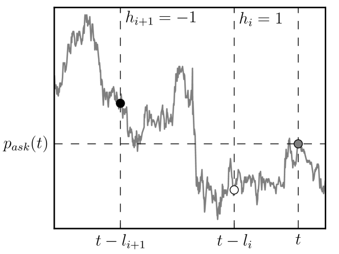
Figure 1: The scheme illustrates specific definition Eq.(3) of the discrete trend variable $h_{i}(t)$ regarding subtraction of he actual exchange rate $p_{\rm ask}(t)$ with foregoing $p_{\rm ask}(t-l_{i})$. The result is encoded by $-1$ or by $1$. In the sense of remark in subsection II.2.2, the situation corresponds to pair of agents operating on the scales $l_{i}$, $l_{i+1}$.

II.2.1 Multi-trend tuple, pattern with participation of many scales

Technical analysis is primarily concerned with identifying patterns of prices that repeat themselves Zunino2009 ; Miller1990 ; Shmilovici2009 . They are mostly based on the symbolic language (lossy encoding) to capture price moves. In further sections we evaluate consequences of the use of N-tuples of primitive discretized trends $h_{i}(t)$ collected to form

$${\bf h}(t)=\left[\,h_{1}(t),h_{2}(t),\ldots,h_{N}(t)\,\right]\,.$$ (5)

This multi-scale TF structures may be eventually seen as specific patterns of alternating type $-1$ and type $+1$ repeats. Their prediction potential will be studied in the next.

II.2.2 Viewing trends as information inputs of autonomous agents

The tuple ${\bf h}(t)$ may be alternatively viewed as instantaneous macrostate variable for the appropriate decision making of the autonomous agents. In the present approach, each agent is provided with the information about $h_{i}(t)$ she/he extracts by measuring the change of the currency rate on its internal specific time scale $l_{i}$.

II.3 The rate changes accounting for bid/ask spread

From the FX trader’s point-of-view, the currency changes may lead to three principally distinct situations which we suggest to be encoded by three-valued variable $S\in\{-1,0,1\}$ we call currency rate shift. It is defined using discretization of exchange rate as follows

$$S(t) = \left\{\begin{array}[]{rcl}-1&,&p_{\rm ask}(t+l_{\rm pr})<p_{\rm bid}(t)\,,\\ +1&,&p_{\rm bid}(t+l_{\rm pr})>p_{\rm ask}(t)\,,\\ 0&,&\mbox{otherwise}\end{array}\right.\,$$ (9)

where $p_{\rm bid}(t)$ is the demand price of particular currency and $l_{\rm pr}$ is the time horizon for which the currency rate change is being transferred to its discrete form. The situation is depicted in Fig. 2. The position is supposed to be held from time $t$ to $t+l_{\rm pr}$. For example, in the case of short selling, the holding period $l_{\rm pr}$ refers to the time between borrowing a currency pair from brokerage, selling it to someone else and then buying it back later. A steep enough currency movement characterized by $|S(t)|=1$ needs to choose appropriate FX operation. It allows the holder of the short position to earn profit from the sale ($S(t)=-1$) or from buying ($S(t)=1$). Clearly, relatively small currency changes are converted to $S(t)=0$. In this case, the position opening (at $t$) causes the loose because of the bid-ask spread. However, an important issue not discussed in the present work is the number of units in the trade.

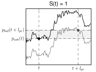
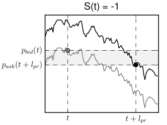
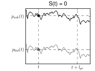
Figure 2: Figure illustrates discretization - currency rate shift $S(t)$ which may attain values $\{-1,0,1\}$ corresponding to different situations as described by Eq.(9).

III Statistical analysis of data

III.1 The correspondence between single trend and $S$

In this section we attempt to answer the question of the relevant time scales for which TF agents come closer to the correct prediction. We came with the proposal of the following conditional statistical matching average

$$\overline{E}_{i}=\frac{1}{\#\{t,S(t)\neq 0\}}\,\sum_{t|S(t)\neq 0}\tilde{\delta}_{[\,h_{i}(t),S(t)]\,}\,,$$ (10)

where $\tilde{\delta}_{[.,.]}$ is defined for two arguments as follows

$$\tilde{\delta}_{[A,B]} = \left\{\begin{array}[]{lcl}+1&,&A=B\\ -1&,&A\neq B\\ \end{array}\right.\,.$$ (13)

Note that measure identifies the coincidence of two-valued $h_{i}(t)$ with a non-zero states of $S(t)$. By measuring of $\overline{E}_{i}$ over the given data for both $h_{i}(t)$ and counter-trend $h_{i}^{-}(t)=-h_{i}(t)$ and their corresponding tuples

$${\bf h}^{-}(t)=-{\bf h}(t)$$ (14)

we obtained $\overline{E}_{i}$ dependencies on $i$, depicted in Fig. 3. The testing of the effect of the counter-trend expresses that current trends can be broken at any time because of arrival of new market information. Surprisingly, when $\overline{E}_{i}$ is calculated for counter-trend the matching becomes larger compared to the matching average calculated for ${\bf h}(t)$.

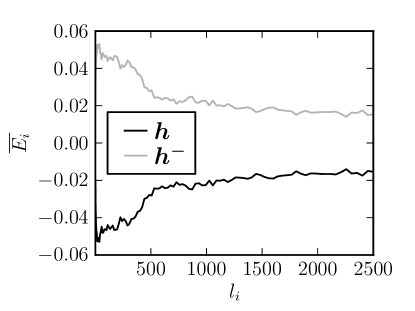
(a)  (b)  (c) 

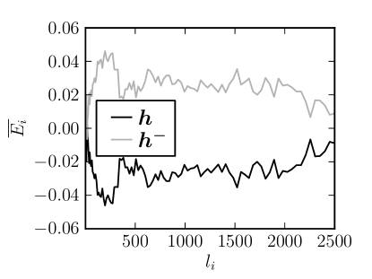
Figure 3: Figure showing $\overline{E}_{i}$ dependence on the time scale $l_{i}$ obtained for (a) $l_{\rm pr}=15$, (b) $l_{\rm pr}=60$, and (c) $l_{\rm pr}=240$. Surprisingly, the positive matching is achieved by the contrarian strategy (counter-trends).

III.2 Multi-trend tuple and consequent $S$

In the previous subsection, we studied relationship of single trend with $S(t)$. The logical extension of former efforts will be the study of the correspondence between ”action” ${\bf h}(t)$ and ”response” $S(t)$. The question arises if the compatibility of many trends (their signs) makes the correspondence more pronounced and satisfying. Here we choose to be less demanding with respect of sign by focussing on the correspondence between the overall effect of trends quantified by the absolute value of instant mean

$$H(t)=\frac{1}{N}\,\Big{|}\sum_{i=1}^{N}h_{i}(t)\Big{|}\,$$ (15)

and $|S(t)|$. The degree of $H(t)$, $|S(t)|$ correspondence may be measured by the conditional average

$$T(\varepsilon)=\frac{1}{\#\{t,H(t)<\varepsilon\}}\,\sum_{t|H(t)<\varepsilon}|S(t)|\,,$$ (16)

where $\#$ denotes the cardinality of the set of events selected according to threshold $H(t)<\varepsilon$. The variable $\varepsilon$ is introduced to control how much homogeneity is in the trends $h_{i}(t)$, $i=1,2,\ldots,N$. Fig. 4 shows the cumulative effect represented by $T(\varepsilon)$. As we can see, the monotonicity of $T(\varepsilon)$ detectable for $l_{\rm pr}=15,60$ min becomes interrupted at $l_{\rm pr}=240$ min, where peak is observed. It seems rather counterintuitive that function $T(\varepsilon)$ is increasing in $l_{\rm pr}$. This fact stems from the relative suppression of $S=0$ states at larger $l_{\rm pr}$, where currency changes become excessive.

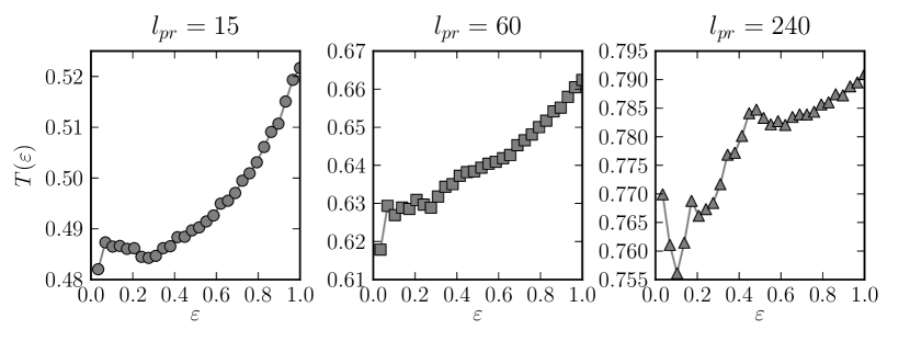
Figure 4: The $T(\varepsilon)$ dependence calculated for different time horizons.

III.3 Similarity of multi-trend tuples and predictability

In this subsection we introduce measure which admits to analyze prediction abilities based on the trend tuples. The basic idea behind can be seen as continuity in the multivariate space of dimension $N$. The dissimilarity between two trend tuples ${\bf h}(t_{i})$ and ${\bf h}(t_{j})$ measured at different moments $t_{i},t_{j}$ may be expressed by means of Hamming-like distance

$$D_{{\rm h},(i,j)}=\sum_{k=1}^{N}\left(\,1-\delta\left(\,h_{k}(t_{i}),h_{k}(t_{j})\right)\,\right)\,,$$ (17)

where $\delta(x,x)=1$, and $\delta(x,y)=0$ as $x\neq y$. Then the statistics may be represented by the histogram of $|S(t_{i})-S(t_{j})|$ differences

$$\psi(r)=\frac{1}{\#\{i,j,D_{{\rm h},(i,j)}=r\,\}}\,\sum_{i,j|\,D_{{\rm h},(i,j)}=r}|S(t_{i})-S(t_{j})|\,.$$ (18)

Note that summation is carried out only for pairs that satisfy constraint $D_{{\rm h},(i,j)}=r$. The assumption of continuity implies monotonic increase of $\psi(r)$ on the $r$ (related to Hamming-like distance) as $r$ is sufficiently small. Other words, similarity of the tuples should imply similarity in the currency rate shifts (see Fig 5). The data analysis show us that monotonicity takes place in the limited $N$, $l_{\rm pr}$ parametric region only, while the combination of large $l_{\rm pr}$ with small $N$ better achieves the expected monotonicity of $\psi(r)$.

We may conclude from this that character of FX data and trading data in general impose restrictions on the overall tuple size and only tuples of the restricted size may be efficient in the reducing of the forecast error $\sim|S(t_{i})-S(t_{j})|$. Results obtained show that the best performance is achieved within the range $12<N<20$ (only three $N$ are plotted due to lack of space).

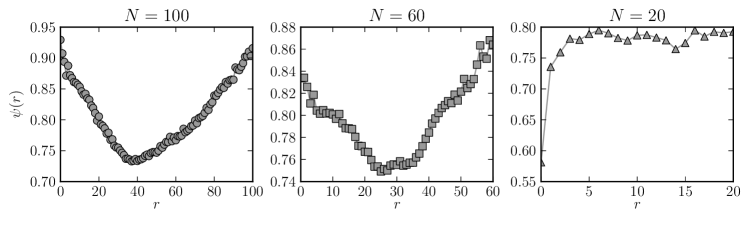
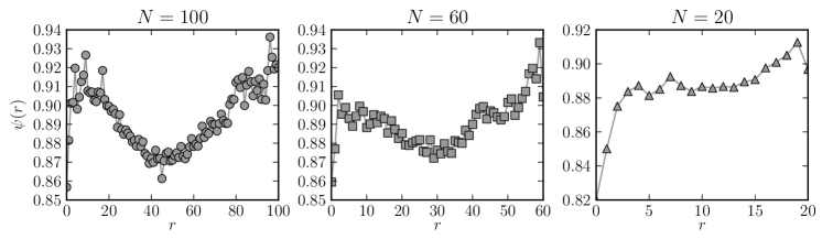
(a)  (b)  (c) 

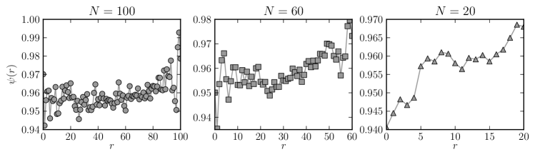
Figure 5: $\psi(r)$ dependence calculated for different time horizons: (a) $l_{\rm pr}=15$ min; (b) $l_{\rm pr}=60$ min; (c) $l_{\rm pr}=240$ min. Among the selected cases, the $N=20$ tuple with monotonously increasing $\psi(r)$ is roughly the most perspective for the forecasting purposes.

IV Conclusions

We investigated statistical properties of TF and multi-TF strategies. We started with elementary TF forms where information comes solely from the difference of two prices (two currencies) separated by the fixed time scale (delay). The study of statistics revealed clear non-suitability of naive trend estimator for the forecast purposes. According to the results obtained, the trend continuation is less good compared to the contrarian strategy of the trend turnover. Similar and quite universal conclusion has been confirmed by the previous studies performed for different market data (including e.g. commodities) which span over different time scales.

The statistical analysis supported development and implementation of parallelized TF strategies build upon the tuple which consists of many trends for contributing time scales. We have shown that one may benefit from the prediction potential of such complex information structures, however, the vast majority of problems remain to be solved. The optimal inter-tuple distance in common with suitable multi-valued trend discretization which regards bid-ask spread could be essential ingredients required for success of such efforts. In such formulation nearly optimal $N$ may play the role of the embedding dimension Grassberger1983 , i.e. minimum number of independent variables necessary to describe system. Intuitively, the parameter $N$ optimized to produce most reliable forecast (including optimization of $l_{\rm pr}$ scale) may be different from the value of ’true’ embedding dimension.

In the future, it would be interesting to experiment with recurrence quantification analysis Marwan2008 ; Bigdeli2009 to characterize complexity in iterations of the multi-trend tuples (patterns) obtained from the time series of generally non-stationary market rate returns.

References

- (1) E.F. Fama, Efficient capital markets: a review of theory and empirical work, J. Financ. 25 (1970) 383-417
- (2) A. Sansone, G. Garofalo, Asset price dynamics in a financial market with heterogeneous trading strategies and time delays, Physica A 382 (2007) 247-257
- (3) B. Afshinpour, G. Ali Hossein-Zadeh, H. Soltanian-Zadeh, Nonparametric trend estimation in the presence of fractal noise: Application to fMRI time-series analysis, Journal of Neuroscience Methods 171 (2008) 340-348
- (4) R.E. Chandler, E.M. Scott (Eds.), Nonparametric trend estimation, in Statistical methods for trend detection and analysis in the environmental sciences, John Wiley & Sons, Ltd, Chichester, UK, 2011.
- (5) R.A. Stevenson, R.M. Bear, Commodity futures: trends or random walks?, Journal of Finance 25 (1970) 65-81
- (6) G. Oh, S. Kim, Ch. Eom, Market efficiency in foreign exchange markets, Physica A 382 (2007) 209-212
- (7) L. Zunino, M. Zanin, B.M. Tabak, D.G. Pérez, O.A. Rosso, Forbidden patterns, permutation entropy and stock market inefficiency, Physica A 388 (2009) 2854-2864
- (8) W. Fung, D.A. Hsieh, The risk in hedge fund strategies: theory and evidence from trend followers, The review of financial studies 14 (2001) 313-341
- (9) J. James, Simple trend-following strategies in currency trading, Quantitative finance 3 (2003) C75-C77
- (10) R.M. Miller, Computer-aided financial analysis, Addision-Wesley, Reading, MA, 1990, pp.314.
- (11) A. Shmilovici, Y. Kahiri, I. Ben-Gal, S. Hauser, Measuring the efficiency of the intraday forex market with a universal data compression algorithm, Computational Economics 33 (2009) 131-154
- (12) P. Grassberger, I. Procaccia, Measuring the strangeness of strange attractors, Physica D: Nonlinear Phenomena 9 (1983) 189-208
- (13) N. Marwan, A historical review of recurrence plots, Eur. Phys. J Special Topics 164 (2008) 3-12
- (14) N. Bigdeli, K. Afshar, Characterization of Iran electricity market indices with pay-as-bid payment mechanism, Physica A 388 (2009) 1577-1592