Adiabatic Evolution of Mass-losing Stars

Abstract

We have calculated the equilibrium properties of a star in a circular, equatorial orbit about a Super-Massive Black Hole (SMBH), when the star fills and overflows its Roche lobe. The mass transfer time scale is anticipated to be long compared with the dynamical time and short compared with the thermal time of the star, so that the entropy as a function of the interior mass is conserved. We have studied how the stellar entropy, pressure, radius, mean density, and orbital angular momentum vary when the star is evolved adiabatically, for a representative set of stars. We have shown that the stellar orbits change with the stellar mean density. Therefore, sun-like stars, upper main sequence stars and red giants will spiral inward and then outward with respect to the hole in this stable mass transfer process, while lower main sequence stars, brown dwarfs and white dwarfs will always spiral outward.

1 Introduction

When a star loses mass on a time scale faster than the Kelvin-Helmholtz time (but slower than the dynamical time), as can happen in Extreme Mass-Ratio Inspirals (EMRI), the structure of the star will evolve adiabatically so that the entropy as a function of interior mass $S(m)$ is approximately conserved. This will be true of radiative and convective zones (except near the surface). Webbink (1985) gave a general introduction to binary mass transfer on various time scales. Hjellming & Webbink (1987) used polytropic stellar models to explore the stability of this adiabatic process, and listed several critical mass ratios above which the donor stars are unstable on dynamical time scales. Soberman et al. (1997) further discussed the stability of binary system mass transfer processes on the thermal and dynamical times scales.

The previous works generally assumed comparable masses of the two objects in the binary system, and an unchanging distance between them throughout the process. In this paper, we will use real stellar models to study how stars respond to the loss of mass adiabatically on a time scale slower than the dynamical time scale but still faster than the thermal one. The star’s orbital radius from the hole is no longer held as a constant. The way that the star evolves in such a mass-transfer environment depends upon the mean density of the stripped star as a function of decreasing mass. Nuclear reactions will be shut off as soon as the mass loss starts, as they are highly temperature-sensitive (Woosley et al., 2002) and the central temperature decreases, at least in the cases that concern us here.

In our EMRI binary system, the star is assumed to be in a circular, equatorial orbit about the central massive black hole. The mass transfer starts when the star just fills its Roche lobe, when materials will flow out of the inner Lagrangian point L1. We call this the Roche mass transfer process. During the mass transfer phase, the stellar orbital radius may increase or decrease. However, we assume that the change is slow enough so that the stellar orbit remains circular. If the orbit crosses the black hole’s innermost stable circular orbit (ISCO) before it is tidally consumed, it will plunge into the hole. The ISCO has radius 6$R_{g}$ for a non-rotating black hole, and 1.237$R_{g}$ for a spin parameter $a=0.998$ black hole (Thorne, 1974). Here $R_{g}$ is the gravitational radius of the hole defined as $GM_{\rm{BH}}/c^{2}$, where $G$ is the gravitational constant, $M_{\rm{BH}}$ is the mass of the black hole, and $c$ is the speed of light.

In this paper we consider the evolution of a representative set of stars and planets under these conditions. In section 2 we discuss the radius-mass relation of a star composed of ideal gas when losing mass adiabatically. In section 3 we study the case of a solar type star. In section 4 we investigate lower main sequence stars, upper main sequence stars, red giants, white dwarfs, brown dwarfs and planets. We will illustrate the use of these evolutionary models in upcoming papers.

After this work was completed, our attention was drawn to a recent paper: Ge et al. (2010). Although the end application of their paper is different, some of the calculations overlap (and agree with) those presented below.

2 Radius-Mass Relation

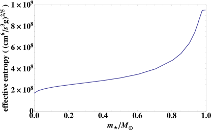
Figure 1: The local entropy of the Sun as a function of its interior mass. The effective entropy is defined as $P^{3/5}\rho^{-1}$. The curve has a flat portion at the upper right, since the entropy is almost constant in the surface convective zone.

For a star composed of ideal gas, we have:

$$\frac{dr}{dm}=\frac{1}{4\pi r^{2}\rho(m)},$$ (1)

where $r$ is the radius, $m$ is the interior mass, and $\rho$ is the density. This gives

$$\frac{dP}{dm}=-\frac{Gm}{4\pi r^{4}},$$ (2)

where $P$ is the gas pressure, and $G$ is the gravitational constant.

Ignoring radiative contributions, Coulomb and degeneracy corrections, the entropy per particle will be $S/N\sim C_{v}\ln\left(P/\rho^{\gamma}\right)$ with $\gamma=5/3$ for ideal monatomic gas, up to a constant; and we can define an effective entropy $\tilde{S}=P^{3/5}\rho^{-1}$ for such an ideal gas.

Then, for a mass-losing star, with constant local entropy, we have

$$\frac{dr}{dm} = \frac{\tilde{S}(m)}{4\pi r^{2}P^{\frac{3}{5}}},$$

$$\frac{dP}{dm} = -\frac{Gm}{4\pi r^{4}}.$$ (3)

For a star with a known entropy profile, we can solve for its new equation of state with boundary conditions that $r_{\star}(0)=0$ and $P_{\star}(0)=P_{0\star}$. We solve for the total stellar mass $M_{\star}$ and the surface radius $R_{\star}=r_{\star}(M_{\star})$, where $P_{\star}(M_{\star})=0$. Then the volume and average density of the star in this new model can be obtained.

Figure 2: The pressure vs interior mass for a mass-losing Sun-like star. The four colored curves represent the four cases when the stellar central pressure decreases to $0.7\ \rm{(blue)},\ 0.4\ \rm{(green)},\ \rm{and}\ 0.1\ \rm{(red)}\ \rm{from}\ 1\ \rm{(purple)}\ P_{0\odot}$.

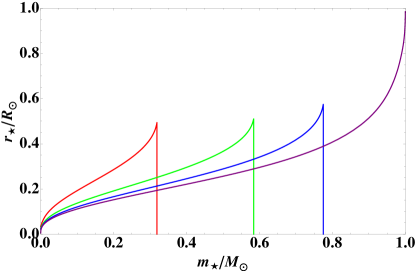
Figure 3: The radius vs interior mass for a mass-losing Sun-like star. The four curves represent the same cases as in Fig. 2.

When the star orbits in a circular equatorial orbit and loses mass under stable evolution during this Roche mass transfer phase, its orbital period will follow $P_{R}\propto{\bar{\rho}_{\star}}^{-1/2}$, where $P_{R}$ is the Roche orbital period, and $\bar{\rho}_{\star}$ is the mean density of the stripped star. This formula can be obtained by comparing the tidal force from the hole and the gravitational force from the star for a point mass on the Roche surface, and also using Kepler’s laws in the Newtonian limits. Through simple calculation we can also get the angular momentum of the system $L_{\star}\sim m_{\star}P_{R}^{1/3}\sim m_{\star}{\bar{\rho}_{\star}}^{-1/6}$, which should decrease for stability throughout the Roche mass transfer phase through slowly gravitational radiation. Here we neglected the much smaller angular momentum carried away by the hot stream flowing out of the inner Lagrangian point (L1). Therefore, the change of ${\bar{\rho}}_{\star}$ and $L_{\star}$ in this adiabatic evolution would allow us to know whether the mass-transfer is stable or catastrophic on the dynamical time scales, and also how the stellar orbit evolves through this process. For example, if the mean density of the star decreases, its orbital period will increase indicating that it is moving farther from the hole. The exact formulas of $P_{R}$ and $L_{\star}$ will be discussed in upcoming papers, in not only the Newtonian limits but also the relativistic limits.

3 Solar Model

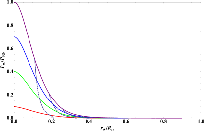
Figure 4: The pressure vs radius for a mass-losing Sun-like star. The four solid curves still represent the cases when a Sun-like star loses its mass until its new central pressure is $P_{0\star}=1,\ 0.7,\ 0.4,$ and $0.1\ P_{0\odot}$, from the top (purple) to the bottom (red). The five blue dashed lines are contours enclosing the same interior mass: $0.1,\ 0.3,\ 0.5,\ 0.7,\ \rm{and}\ 0.9\ M_{\odot}$ from left to right respectively. (The two rightmost lines are very hard to see). We can observe that as the star loses its mass, the surface pressure of any shell decreases and that shell enclosing constant mass expands.

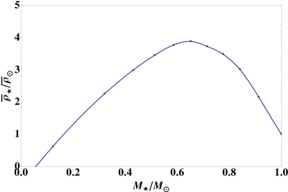
Figure 5: The mean density of a star with decreasing total mass for a Sun-like star. The blue solid curve is an interpolation of the red data points for $P_{0\star}=0.01,\ 0.1,\ 0.2,\ 0.3,\ 0.4,$ $0.5,\ 0.6,\ 0.7,\ 0.8,\ 0.9\$ and $1\ P_{0\odot}$ from left to right.

Let us start with the Sun as a representative example of main sequence stars. We adopted Guenther and Demarque’s standard solar model (Demarque et al. (2008); Guenther & Demarque (1997)) to derive $\tilde{S}(m)$ as in Fig.1. Notice that the entropy is almost constant for the outer thirty percent of its radius, which corresponds to the convective zone of the Sun.

Using the entropy profile, we computed the radius of the star $r_{\star}$ and the pressure of the star $P_{\star}$ as functions of the interior mass $m_{\star}$, when the star is adiabatically evolved to a new equilibrium. We plotted $r_{\star}(m_{\star})$, $P_{\star}(m_{\star})$,and $P_{\star}(r_{\star})$ in Fig.2, Fig. 3, and Fig.4, as the star loses mass to the point that the central pressure equals $0.7,\ 0.4,\ 0.1$ from the original stellar central pressure $P_{0\odot}$. As the mass of the star is stripped, its interior pressure decreases and total radius shrinks.

As the mass of a Sun-like star decreases, its central pressure also decreases. By observing contour lines of the constant interior masses in Fig.4, we can see that shells enclosing the constant masses are expanding in this evolution.

The total stellar volume, however, is still almost monotonically decreasing in this evolution. For a solar model, the volume contracts first and then remains almost constant. Therefore its mean density increases first and then drops. We can observe the change of the stellar mean density as the mass decreases in Fig. 5. For the first $\sim 40\%$ of the solar mass, the star moves closer to the hole since the density is increasing, then the star moves farther from the hole for the rest of the Roche mass transfer phase.

Lastly we want to check whether this Roche process is stable or not. By plotting the effective angular momentum $L_{\star}$ as a function of the rest total stellar mass $M_{\star}$ as in Fig. 6, we confirmed that $L_{\star}$ does decrease. The mass transfer is stable on a dynamical time scale.

Figure 6: The effective angular momentum $L_{\star}$ of the star with decreasing total mass for a Sun-like star. $L_{\star}$ is defined as $M_{\star}\bar{\rho}_{\star}^{-1/6}$, and $L_{\odot}$ is defined as $M_{\odot}\bar{\rho}_{\odot}^{-1/6}$. The data points represent the same cases as in Fig. 5.

4 Other Stars

4.1 Lower Main Sequence Stars

Lower main sequence stars have different structures from the Sun. The whole star is convective and has almost constant entropy (e.g., Girardi et al. (2000); Padmanabhan (2001)). Here we chose a star with $\sim 0.3$ stellar mass as a representative. We adopted models computed by one os us (PE) for other purposes. All these zero age main sequence stars have metalicity $Z=0.01$.

Figure 7: The radius vs interior mass for a mass-losing lower main sequence star with $\sim 0.3M_{\odot}$ mass. The four colored curves represent the four cases when the stellar central pressure equals $0.1\ \rm{(red)},\ 0.4\ \rm{(green)},\ 0.7\ \ \rm{(blue)},\ \rm{and}\ 1\ \rm{(purple)}$ original stellar central pressure.

As the star loses its mass, it expands and its interior pressure decreases, similar to the solar case. The radius-mass relation (Fig. 7) shows that the major difference between this model and the solar model is that the total volume of a low-mass star is always monotonically increasing. Therefore, its mean density will continue to decrease in the Roche phase (Fig. 8). A lower main sequence star will move out as it transfers mass. The effective angular momentum for this star however decreases throughout the Roche mass transfer phase due to the loss of mass, confirming that the star is stripped stably on the dynamical time scale.

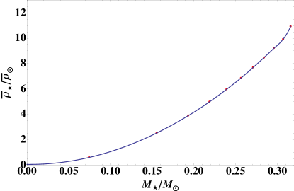
Figure 8: The stellar mean density with decreasing total mass for a lower main sequence ($\sim 0.3M_{\odot}$) star. The blue solid curve is an interpolation of the red data points representing $P_{0\star}=0.01,\ 0.1,\ 0.2,\ 0.3,\ 0.4,\ 0.5,\ 0.6,\ 0.7,\ 0.8,\ 0.9$ and $1$ original stellar central pressure, from left to right.

4.2 Upper Main Sequence Stars

Upper main sequence stars have convective cores for more efficient energy transport (e.g., Woosley et al. (2002)). This mixing of material around the core removes the helium ash from the hydrogen burning region, allowing more of the hydrogen in the star to be consumed during the main sequence lifetime. Therefore the local effective entropy is almost constant in the center. The outer regions of a massive star are radiative. We investigated a $\sim 7.9\ M_{\odot}$ star as an example.

The mean density of an upper main sequence star behaves similarly to the solar case, as shown in Fig. 9. An upper main sequence star will first move in and then out, while stably filling its Roche lobe in the mass-accreting phase, since its angular momentum can be calculated as decreasing as well.

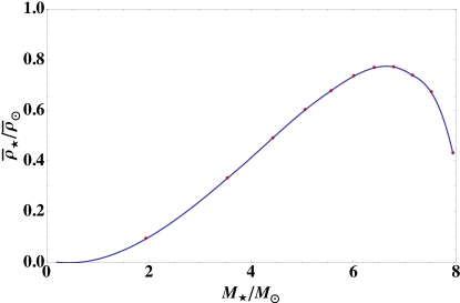
Figure 9: The stellar mean density with decreasing total mass for an upper main sequence star with $\sim 7.9M_{\odot}$ mass). The blue solid curve is an interpolation of the red data points representing $P_{0\star}=0.01,\ 0.1,\ 0.2,\ 0.3,\ 0.4,\ 0.5,\ 0.6,\ 0.7,\ 0.8,\ 0.9$ and $1$ original stellar central pressure, from left to right.

4.3 Red Giants

Main sequence stars above $0.5\ M_{\odot}$ evolve into red giants in their late phases (Reimers, 1975; Sweigart & Gross, 1978). Here we actually used a red supergiant with $11.85\ M_{\odot}$ to study how it reacts to the loss of mass due to tidal stripping. Its effective entropy, defined in the same manner as before, is shown in Fig. 10. We can see a carbon-helium core with higher density and a much less dense hydrogen shell with $\sim 6\ M_{\odot}$ mass inside.

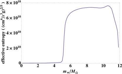
Figure 10: The local entropy of a red supergiant of mass $11.85\ M_{\odot}$ as a function of the stellar interior mass. A carbon core resides mostly within $\sim 2.7\ M_{\odot}$, followed by a helium core lasting untill $\sim 6\ M_{\odot}$. The entropy for the hydrogen shell outside is much higher due to its low density.

The pressure - mass, radius - mass, and pressure - radius relations are also plotted in Fig.11, Fig.12, and Fig. 13. We can observe that red giants have pressure-mass curves with much steeper gradients compared with main sequence stars, and very extended low-density hydrogen outer layers. When this hydrogen shell is fed to the SMBH very rapidly, the central pressure is not affected much. In that regime, the response of the star is not strictly adiabatic.

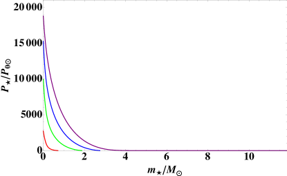
Figure 11: The pressure vs interior mass for the red supergiant of Fig. 10. The four curves are cases when the stellar central pressure equals $0.1\ \rm{(red)},\ 0.4\ \rm{(green)},\ 0.7\ \ \rm{(blue)},\ \rm{and}\ 1\ \rm{(purple)}$ of the original central pressure. The pressure decreases very fast going from the center of the star to its surface. There is a very extended hydrogen outer layer with relatively much lower density, as can be seen from the purple curve.

We also plotted Fig. 14 to see how the mean density of the red giant changes with its total mass. The star’s total volume shrinks by a factor bigger than a thousand as the hydrogen envelope is consumed, therefore the mean density increases a lot at the beginning and then starts to decrease. The red giant is stably stripped, while first moving in and then out.

A star is a red giant for only a small fraction ($10\%$ to $25\%$) of its fusion lifetime (e.g., Padmanabhan (2001)). Therefore, it would be rare to observe a red giant feeding an SMBH accretion disc.

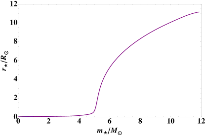
Figure 12: The radius vs interior mass for the red supergiant of Fig. 10. The four cases correspond to the same models as in Fig. 11. We can see that the volume of the red supergiant shrinks a lot soon after the tidal stripping starts. Also losing the hydrogen photosphere leaves the central region of the star almost unaffected.

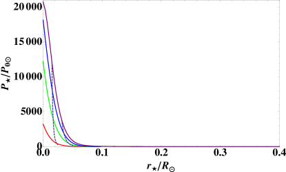
Figure 13: The pressure vs radius profile of a mass-losing red supergiant with total initial mass $11.85\ M_{\odot}$. Here the dashed lines represent the shell enclosing $0.02\ M_{\star}$ (left) and $0.1\ M_{\star}$ (right).

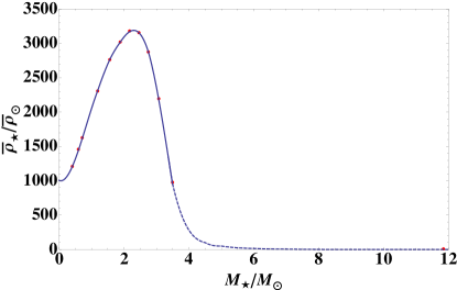
Figure 14: The mean stellar density with decreasing total mass for a red supergiant with total initial mass $11.85\ M_{\odot}$. The red data points stand for $P_{0\star}$ equals $0.05,\ 0.08,\ 0.1,\ 0.2,\ 0.3,\ 0.4,\ 0.5,\ 0.6,\ 0.7,\ 0.8,\ 0.9$ and $1$ original stellar central pressure. The mean densities for $M3.5M_{\odot}$ are probably inaccurate owing to the relative fragility of the red giant envelope.

4.4 White Dwarfs

White dwarfs are composed of a nondegenerate gas of ions and a degenerate and at least partly relativsitc gas of electrons (Kippenhahn & Weigert, 1994). We need to redefine its effective entropy since the entropy of a degenerate electron gas differs from that of a nondegenerate gas. However, an easier way of obtaining the structure of the evolved white dwarf would be just to use its radius-mass relation:

$$R_{\star}(M_{\star})\simeq 0.022\mu_{e}^{-1}R_{\odot}\left(\frac{M_{\star}}{M_{\rm{ch}}}\right)^{-\frac{1}{3}}\left[1-\left(\frac{M_{\star}}{M_{\rm{ch}}}\right)^{\frac{4}{3}}\right]^{\frac{1}{2}}$$ (4)

(Nauenberg, 1972). In this equation, $R_{\star}$ and $M_{\star}$ are the total radius and mass of the evolved white dwarf. $\mu_{e}$ is the average number of nucleons per electron, and $\mu_{e}=2$ for He, C, O, which is also a good approximation for most other options. $M_{\rm{ch}}$ is the Chandrasekhar mass, which is approximately $1.459M_{\odot}$. The formula holds true, except when the stellar mass is close to its upper limit $M_{\rm{ch}}$, where the radius should approach a constant.

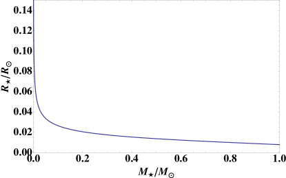
Figure 15: The total radius as a function of the total mass for a white dwarf, as the total mass decreases from $\bf{1M_{\odot}}$ to zero. We can see that the less massive a white dwarf is, the larger its volume actually is.

We consider a $1M_{\odot}$ white dwarf with complete degeneracy and zero temperature, and show its radius-mass and mean density-mass relations in Fig. 15 and Fig.16. As the white dwarf is tidally stripped, its total volume increases in this adiabatic evolution, ensuring that the mean stellar density decreases throughout the Roche phase. Therefore, as a white dwarf loses its mass under the Roche process, it will always expand its orbit.

For a white dwarf with a mass close to $M_{\rm{ch}}$, its radius does not change much as it loses mass, so the effective angular momentum ($L_{\star}\propto M_{\star}\bar{\rho_{\star}}^{-1/6}\propto M_{\star}^{5/6}$) decreases throughout the Roche mass-transfer phase. Adiabatic mass-transfer is stable on the dynamical time scale for all types of white dwarfs.

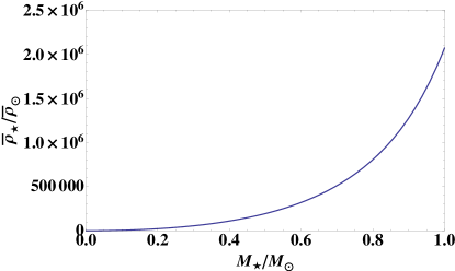
Figure 16: The stellar mean density of a white dwarf, as its total mass decreases from $1M_{\odot}$ to zero. As its mass is stripped, its mean density decreases.

4.5 Brown Dwarfs

Brown dwarfs never undergo hydrogen reactions. They are supported by the degeneracy pressure of their non-relativistic electrons (Kippenhahn & Weigert, 1994). Their ions are treated as ideal gases. Brown dwarfs are also fully convective.

The total pressure of a brown dwarf, including the ideal ion gas pressure and the electron degeneracy pressure, goes as:

$$P\simeq K\rho^{\frac{5}{3}},$$ (5)

where $K$ is a constant close to $10^{13}$ dyn cm^-2 (e.g., Padmanabhan (2001); Burrows & Liebert (1993); Burrows et al. (2001); Burrows et al. (2002); and the references therein). The effective entropy, still defined as $P^{3/5}\rho^{-1}$, therefore would be a constant, confirming the convective structure.

Using the relation between $P$ and $\rho$, we can solve the equations of equilibrium [eq. (2)] for a brown dwarf with a certain new central density and total mass. Here we used a 1 Gyr brown dwarf with total mass $0.05M_{\odot}$ with central density $458.0$ g cm^-3 and total radius $6.4\times 10^{9}$ cm (Burrows & Liebert, 1993). K is calculated to be $\sim 8.5\times 10^{12}$ dyn cm^-2, in order to fit the model. Using our routine, we show how the mean stellar density varies with total mass in Fig. 17. The brown dwarf, therefore, moves outward from the hole as its mass is tidally stripped. Its effective angular momentum also decreases monotonically, so this process is stable on the dynamical time scale.

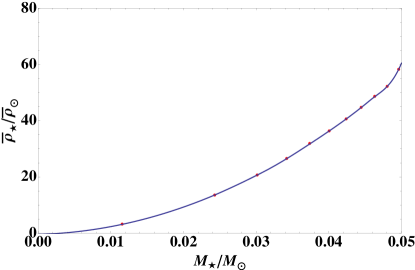
Figure 17: The stellar mean density as a function of its total mass for a brown dwarf, as its total mass decreases from $0.05M_{\odot}$ to zero. We can see that the less massive a brown dwarf is, the less dense it is in this adiabatic evolution. The red data points were obtained using the model with $P_{0\star}=0.01,\ 0.1,\ 0.2,\ 0.3,\ 0.4,\ 0.5,\ 0.6,\ 0.7,\ 0.8,\ 0.9$,  and $1$ original stellar central pressure, from left to right, and the blue solid curve is an interpolation of these data points.

4.6 Planets

Planets like Jupiter (Baraffe et al., 2008; Nettelmann et al., 2008) have complex structures. However, we can study two extreme cases, namely, completely solid planets and completely liquid ones, in order to see how they react to tidal consumption by a massive hole.

The densities of solid planets like Earth will remain unchanged when the planets are tidally stripped. And these planets tend to have relatively similar densities from the center to the surface. Therefore, the mean densities of such planets do not change, and the stellar orbital periods do not change either.

Liquid planets (even with a solid core) are self-gravitating spheres following polytropic models. For such a planet, its pressure and density roughly follows $P=K\rho^{1+1/n}$, where $K$ is a constant, and the polytropic index $n=1$ in this case (Kippenhahn & Weigert, 1994). As the planet is stripped, it still follows the polytropic model and satisfies the hydrostatic equations (1) and (2). Therefore we can do simple calculations to obtain the new total radius $R_{p}$ of the planet:

$$R_{p}=\sqrt{\frac{\pi K}{2G}}.$$ (6)

In other words, the total radius of the planet remains the same all through the stable tidal stripping process. So the mean density of the planet decreases, meaning that the planet moves out as mass is stripped. Its effective angular momentum decreases as well.

5 Discussion

The primary motivation for this paper is to understand the response of a star or a planet when it is tidally stripped by a massive black hole in a stable manner. Such a situation can arise when a star or a planet is formed in an accretion disc, and then evolves through circular orbits of diminishing radius under the action of gravitational radiation. (Other capture scenarios are possible, and have been widely discussed in the literature (Novikov et al., 1992; Sigurdsson & Rees, 1997; Alexander & Livio, 2004).)

We constrained the orbit to be circular for simplicity, because of the rapid decay of the stellar orbital eccentricity as angular momentum and energy are carried away by gravitational radiation. Peters (1964) gave a detailed calculation of this, and showed how the eccentricity changes as the orbit shrinks in the decay of a two-point mass system:

$$a_{r}=\frac{c_{0}\ e^{\frac{12}{19}}}{1-e^{2}}\left(1+\frac{121}{304}e^{2}\right)^{\frac{870}{2299}},$$ (7)

where $a_{r}$ is the semi-major axis, $e$ is the eccentricity, and $c_{0}$ is a constant determined by the initial condition $a_{r}={a_{r}}_{0}$ when $e=e_{0}$. Fig. 18 shows how $e$ varies with $a_{r}$ for a set of different initial conditions.

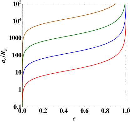
Figure 18: The semi-major axis $a_{r}$ as a function of the eccentricity $e$ in the decay of a two-point mass system, on a log-log scale. Four different colors represent four different initial conditions. We set ${a_{r}}_{0}$ to be at $10^{5}R_{g}$. Then the initial $e_{0}$’s are (from bottom to top): 0.9999 (red), 0.999 (blue), 0.99 (green), and 0.9 (orange).

What is clear from these results is that for most types of stars, the stellar mean density decreases as mass is tidally stripped, at least during the later phase of the mass-transfer. This, in turn, implies that the orbit will expand after mass transfer is initiated. The further implications of this general result will be discussed in a forthcoming paper.

A star in a circular equatorial orbit outside the innermost stable circular orbit (ISCO) of the hole will not be swallowed by the hole. The ISCO of a black hole of mass $M$ and spin $a$ has radius $R_{\rm{ISCO}}$ that satisfies the equation:

$$\left(\frac{R_{\rm{ISCO}}}{M}\right)^{2}-6\frac{R_{\rm{ISCO}}}{M}+8a\sqrt{\frac{R_{\rm{ISCO}}}{M}}-3a^{2}=0$$ (8)

(Bardeen et al., 1972). The ISCO resides between $R_{g}$ (prograde with maximal spin) and $9R_{g}$ (retrograde with maximal spin).

The tidal radius $r_{T}$ for a star with a mass $M_{\star}$ and radius $R_{\star}$ near the hole is (Rees, 1988):

$$r_{T}=5\times 10^{12}\left(\frac{M}{10^{6}M_{\odot}}\right)^{\frac{1}{3}}\frac{R_{\star}}{R_{\odot}}\left(\frac{M_{\star}}{M_{\odot}}\right)^{-\frac{1}{3}}{\rm cm}\ .$$ (9)

For a particular black hole, only stars with their tidal radii smaller than the ISCO of the hole can get very close to the hole before they are tidally disrupted. For example, we can see from Fig. 2 of Dai et al. (2010) that for a $10^{7}M_{\odot}$ black hole, only dwarf stars or lower main sequence stars can get to the ISCO before being tidally disrupted.

Also when the tidal stripping starts, the Roche stellar orbital radius $r_{\rm{R}}$ should be larger than the ISCO of the hole. We shall show in an upcoming paper that $\bar{\rho}_{\rm{R}}=M_{\rm{BH}}/(0.683r_{\rm{R}}^{3})$, where $\bar{\rho}_{\rm{R}}$ and $r_{\rm{R}}$ are the mean stellar density and orbital radius of the star fulfilling the Roche condition. In other words,

$$r_{\rm{R}}\sim 1.27*10^{13}*\left(\frac{M_{\rm{BH}}}{10^{6}M_{\odot}}\right)^{\frac{1}{3}}\left(\frac{\bar{\rho}_{\star}}{\bar{\rho}_{\odot}}\right)^{-\frac{1}{3}}\rm{cm}.$$ (10)

This radius is just slightly larger than $r_{T}$ with the same order of magnitude.

Fig. 19 shows how the Roche radius varies with the central massive black hole mass and the different materials of stars. We use the set of stars that we discuss in this paper. The Roche radius decreases as the star becomes denser, or as the hole becomes more massive for most stars or planets. Also this plot shows a comparison between a star’s Roche radius and the ISCO radius of an SMBH. We can see that, for example, the Sun would fill its Roche lobe at a few gravitational radii for a $10^{7}M_{\odot}$ SMBH; red giants would always be disrupted before they reach the ISCO of SMBHs; and white dwarfs wouldl be tidally disrupted at a few gravitational radii for a $10^{5}M_{\odot}$ black hole.

If the mass transfer is initiated when the star is in a relativistic orbit, the resulting periodic emission may be detectable by X-ray telescopes, which we will discuss in forthcoming papers. Furthermore the behavior of the star could, in principle, be monitored as an “EMRI” source for by a future space-borne gravitational radiation detector.

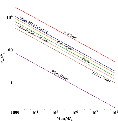
Figure 19: The Roche radius vs central black hole mass for various stars. From top to bottom: a red supergiant with a mass $11.85M_{\odot}$ (red), an upper main sequence star with a mass $\sim 7.9M_{\odot}$ (blue), a Sun-like star (orange), a planet like earth (green), a lower main sequence star with a mass $\sim 0.3M_{\odot}$ (pink), a brown dwarf with a mass $0.05M_{\odot}$ (brown), and a solar mass white dwarf (purple). A planet like Jupiter has a Roche radius similar to that of the Sun-like stars, since their mean densities are similar.

References

- Alexander & Livio (2004) Alexander T., Livio M., 2004, APJ, Part 2 - Letters, 606, L21
- Baraffe et al. (2008) Baraffe I., Chabrier G., Barman T., 2008, Ann. Phys. (Paris), 482, 315
- Bardeen et al. (1972) Bardeen J. M., Press W. H., Teukolsky S. A., 1972, APJ, 178, 347
- Burrows et al. (2002) Burrows A., Burgasser A. J., Kirkpatrick J. D., Liebert J., Milsom J. A., Sudarsky D., Hubeny I., 2002, APJ, 573, 394
- Burrows et al. (2001) Burrows A., Hubbard W. B., Lunine J. I., Liebert J., 2001, Reviews of Modern Physics, 73, 719
- Burrows & Liebert (1993) Burrows A., Liebert J., 1993, Reviews of Modern Physics, 65, 301
- Dai et al. (2010) Dai L. J., Fuerst S. V., Blandford R., 2010, MNRAS, 402, 1614
- Demarque et al. (2008) Demarque P., Guenther D. B., Li L. H., Mazumdar A., Straka C. W., 2008, Astrophys. Space. Sci., 316, 31
- Ge et al. (2010) Ge H., Hjellming M. S., Webbink R. F., Chen X., Han Z., 2010, APJ, 717, 724
- Girardi et al. (2000) Girardi L., Bressan A., Bertelli G., Chiosi C., 2000, Astronomy & Astrophysics, Supplement, 141, 371
- Guenther & Demarque (1997) Guenther D. B., Demarque P., 1997, APJ, 484, 937
- Hjellming & Webbink (1987) Hjellming M. S., Webbink R. F., 1987, APJ, 318, 794
- Kippenhahn & Weigert (1994) Kippenhahn R., Weigert A., 1994, Stellar Structure and Evolution
- Nauenberg (1972) Nauenberg M., 1972, APJ, 175, 417
- Nettelmann et al. (2008) Nettelmann N., Holst B., Kietzmann A., French M., Redmer R., Blaschke D., 2008, APJ, 683, 1217
- Novikov et al. (1992) Novikov I. D., Pethick C. J., Polnarev A. G., 1992, MNRAS, 255, 276
- Padmanabhan (2001) Padmanabhan T., 2001, Theoretical Astrophysics, Volume 2: Stars and Stellar Systems
- Peters (1964) Peters P. C., 1964, Phys. Rev., 136, B1224
- Rees (1988) Rees M. J., 1988, Nature, 333, 523
- Reimers (1975) Reimers D., 1975, Memoires of the Societe Royale des Sciences de Liege, 8, 369
- Sigurdsson & Rees (1997) Sigurdsson S., Rees M. J., 1997, MNRAS, 284, 318
- Soberman et al. (1997) Soberman G. E., Phinney E. S., van den Heuvel E. P. J., 1997, Ann. Phys. (Paris), 327, 620
- Sweigart & Gross (1978) Sweigart A. V., Gross P. G., 1978, The Astrophysical Journal, Supplement, 36, 405
- Thorne (1974) Thorne K. S., 1974, APJ, 191, 507
- Webbink (1985) Webbink R. F., 1985, Stellar evolution and binaries. pp 39–+
- Woosley et al. (2002) Woosley S. E., Heger A., Weaver T. A., 2002, Reviews of Modern Physics, 74, 1015