Normalized Mutual Information to evaluate overlapping community finding algorithms

Abstract

Given the increasing popularity of algorithms for overlapping clustering, in particular in social network analysis, quantitative measures are needed to measure the accuracy of a method. Given a set of true clusters, and the set of clusters found by an algorithm, these sets of clusters must be compared to see how similar or different the sets are. A normalized measure is desirable in many contexts, for example assigning a value of 0 where the two sets are totally dissimilar, and 1 where they are identical.

A measure based on normalized mutual information, [1], has recently become popular. We demonstrate unintuitive behaviour of this measure, and show how this can be corrected by using a more conventional normalization. We compare the results to that of other measures, such as the Omega index [2].

A C++ implementation is available online.

In a non-overlapping scenario, each node belongs to exactly one cluster. We are looking at overlapping, where a node could belong to many communities, or indeed to no clusters. Such a set of clusters has been referred to as a cover in the literature, and this is the terminology that we will use.

For a good introduction to our problem of comparing covers of overlapping clusters, see [2]. They describe the Rand index, which is defined only for disjoint (non-overlapping) clusters, and then show how to extend it to overlapping clusters. Each pair of nodes is considered and the number of clusters in common between the pair is counted. Even if a typical node is in many clusters, it’s likely that a randomly chosen pair of nodes will have zero clusters in common. These counts are calculated for both covers and the Omega index is defined as the proportion of pairs for which the shared-cluster-count is identical, subject to a correction for chance.

I Mutual information

Meila [3] defined a measure based on mutual information for comparing disjoint clusterings. Lancichinetti et al. [1] proposed a measure also based on mutual information, extended for covers. This measure has become quite popular for comparing community finding algorithms in social network analysis. It is this measure we are primarily concerned with there, and we will refer to it as $\mbox{NMI}_{LFK}$after the authors’ initials.

We are proposing to use a different normalization to that used in $\mbox{NMI}_{LFK}$, but first we will define the non-normalized measure which is based very closely on that in $\mbox{NMI}_{LFK}$. You may want to compare this to the final section of Lancichinetti et al. [1].

Given two covers, $X$ and $Y$, we must first see how to measure the similarity between a pair of clusters. $X$ and $Y$ are matrices of cluster membership. There are $n$ objects. The first cover has $K_{X}$ clusters, and hence $X$ is an $n\times K_{X}$ matrix. $Y$ is an $n\times K_{Y}$ matrix. $X_{im}$ tells us whether node $m$ is in cluster $i$ in cover $X$.

To compare cluster $i$ of the first cover to cluster $j$ of the second cover, we compare the vectors $X_{i}$ and $Y_{j}$. These are vectors of ones and zeroes denoting which clusters the node is in.

• ${a=\sum_{m=1}^{n}[X_{im}=0\wedge Y_{jm}=0]}$

• ${b=\sum_{m=1}^{n}[X_{im}=0\wedge Y_{jm}=1]}$

• ${c=\sum_{m=1}^{n}[X_{im}=1\wedge Y_{jm}=0]}$

• ${d=\sum_{m=1}^{n}[X_{im}=1\wedge Y_{jm}=1]}$

If $a+d=n$, and therefore $b=c=0$, then the two vectors are in complete agreement.

The lack of information between two vectors is defined:

$$H(X_{i}|Y_{j})= {}H(X_{i},Y_{j})-H(Y_{j})$$

$$= {}h(a,n)+h(b,n)+h(c,n)+h(d,n)$$

$${}-h(b+d,n)-h(a+c,n)$$ (1)

where $h(w,n)=-w\log_{2}\frac{w}{n}$.

There is an interesting technicality here. Imagine a pair of clusters but where the memberships have been defined randomly. There is a possibility that there will be a small amount of mutual information, even in the situation where the two vectors are negatively correlated with each other. In extremis, if the two vectors are near complements of each other, mutual information will be very high. We wish to override this and define that there is zero mutual information in this case. This is defined in equation (B.14) of [1]. We also use this restriction in our proposal.

$$\begin{split}H^{*}&(X_{i}|Y_{j})=\\ &\left\{\begin{split}H(X_{i}|Y_{j})\;&\mbox{~{}if}\;h(a,n)+h(d,n)\geq h(b,n)+h(c,n)\\ h(c+d,n)+h(a+b,n)\;&\mbox{~{}otherwise}\end{split}\right.\end{split}$$ (2)

This allows us to compare vectors $X_{i}$ and $Y_{j}$, but we want to compare the entire matrices $X$ and $Y$ to each other. We will follow the approximation used by [1] here and match each vector in $X$ to its best match in $Y$,

$$H(X_{i}|Y)=\underset{j\in\{1,\dots K_{Y}\}}{\min}H^{*}(X_{i}|Y_{j})$$ (3)

then summing across all the vectors in $X$,

$$H(X|Y)=\sum_{i\in\{1,\dots K_{X}\}}H(X_{i}|Y)$$ (4)

$H(Y|X)$ is defined in a similar way to $H(X|Y)$, but with the roles reversed. We will also need to define the (unconditional) entropy of a cover,

$$H(X) =\sum_{i=1}^{K_{X}}H(X_{i})$$

$$=\sum_{i=1}^{K_{X}}\left(h\left(\sum_{m=1}^{n}[X_{im}=1],n\right)+h\left(\sum_{m=1}^{n}[X_{im}=0],n\right)\right)\;,$$

where $\sum_{m=1}^{n}[X_{im}=1]$ counts the number of nodes in cluster $i$, end $\sum_{m=1}^{n}[X_{im}=0]$ counts the number of nodes not in cluster $i$,

II Useful identities

Figure 1: Mutual information and variation of information. The total information $H(X,Y)=H(X|Y)+I(X:Y)+H(Y|X)$.

fig. 1 gives us an easy way to remember the following useful identities, which apply to any mutual information context.

$$H(X)= I(X:Y)+H(X|Y)$$

$$H(Y)= I(X:Y)+H(Y|X)$$

$$H(X,Y)= H(X)+H(Y|X)$$

$$H(X,Y)= H(Y)+H(X|Y)$$

$$H(X,Y)= \overbrace{I(X:Y)}^{\text{mutual information}}+\overbrace{H(X|Y)+H(Y|X)}^{\text{variation of information}}$$

The first two equalities give us two definitions for the mutual information, $I(X:Y)$. In theory, these should be identical, but due to the approximation used in eq. 3 they may be different. Therefore, we will use the average of the two.

$$I(X:Y):=\frac{1}{2}\left[H(X)-H(X|Y)+H(Y)-H(Y|X)\right]$$ (5)

We are now ready to discuss normalization, contrasting the method of [1] with our alternative.

Lancichinetti et al. [1] define their own normalization of the variation of information,

$$\frac{1}{2}\left(\frac{H(X|Y)}{H(X)}+\frac{H(Y|X)}{H(Y)}\right)$$ (6)

and hence their normalized mutual information is

$$\mbox{NMI}_{LFK}=1-\frac{1}{2}\left(\frac{H(X|Y)}{H(X)}+\frac{H(Y|X)}{H(Y)}\right)$$ (7)

There are of course many ways to normalize a quantity such as the variation of information. Normalization typically involves division by a quantity $c$,

$$\frac{H(X|Y)+H(Y|X)}{c(X,Y)}$$ (8)

where $c$ is a function of $X$ and $Y$ which is guaranteed to be greater than or equal to the numerator. But $\mbox{NMI}_{LFK}$does not use a normalization of this standard form, instead using eq. 6.

There is another aspect to the non-standard normalization used in $\mbox{NMI}_{LFK}$; they insert an extra normalization factor into their definition of $H(X_{i}|Y_{j})$. But this is not the root cause of the problems we will describe, hence we will not dwell on it. Our change is to remove all the normalization steps from their analysis and instead use a more conventional normalization of the form of eq. 8.

III Unintuitive behaviour

There are circumstances where $\mbox{NMI}_{LFK}$overestimates the similarity of two clusters. We will show how an alternative normalization will fix these problems.

Imagine a cover $X$, and we are comparing it to a cover $Y$. Further, imagine $Y$ has only one cluster ($K_{Y}=1$) and this cluster is identical to one of the clusters in $X$. For large $K_{X}$, we would expect the normalized mutual information to be quite low. An intuitive result would be approximately $\frac{1}{K_{X}}$.

However, $\mbox{NMI}_{LFK}(X,Y)$ will be at least $0.5$ in cases like this. This is because $H(Y|X)$ will be zero bits (the single cluster in $Y$ can be encoded with zero bits because it has a perfect match among the clusters of $X$) and this will result in a contribution of $0.5$ to the $\mbox{NMI}_{LFK}$.

The other problematic example involves the power set. There are $n$ objects in total. A cover involving every subset of the $n$ objects will create $2^{n}-1$ clusters; we will ignore the empty subset. This is the power set, which we denote as $p(n)$.

$\mbox{$\mbox{NMI}_{LFK}$}(X,p(n))$ will again be slightly greater than $0.5$. This is because every cluster in $X$ will have a perfect match in $p(n)$ and this will result in $H(X|p(n))=0$.

In both these examples $\mbox{NMI}_{LFK}$ gives a score slightly above $0.5$. The intuitive behaviour in these cases would be for a similarity score close to $0$. We will demonstrate this behaviour in our experiments in section V

When we remove the normalization from $\mbox{NMI}_{LFK}$, and instead use a more conventional normalization strategy eq. 8, we will find more intuitive behaviour.

IV normalization

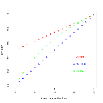
Figure 2: As more communities are found, the scores of $\mbox{NMI}_{LFK}$and $\text{NMI}_{max}$ increase. For a small number of communities found, the intuitive result is a small value, and this is the behaviour of our proposed measure.

Typically a normalization will involve a simple division of the absolute quantity by a quantity which is gauranteed to be an upper bound, giving us a number between zero and one.

The following sequence of inequalities from Vinh et al. [4] provide possibilities for normalization.

$$\begin{split}I(X:Y)\leq&\min(H(X),H(Y))\\ \leq&\sqrt{H(X),H(Y)}\\ \leq&\frac{1}{2}\left(H(X)+H(Y)\right)\\ \leq&\max(H(X),H(Y))\\ \leq&H(X,Y)\end{split}$$ (9)

Any of the five expressions on the right can be used, and [4] suggest a measure based on $\max(H(X),H(Y))$. The Normalized Information Distance is recommended

$$d_{max}=1-\frac{I(X,Y)}{\max(H(X),H(Y))}$$

where zero means perfect similarity and one means dissimilarity. We want a measure with the opposite behaviour, so we’ll use the corresponding normalized mutual information

$$NMI_{max}=\frac{I(X:Y)}{\max(H(X),H(Y))}$$ (10)

where $I(X:Y)$ is as defined in eqs. 2, 3, 4 and 5

This can also be understood with reference to fig. 1. The problem with $\mbox{NMI}_{LFK}$ arises when one cover is more complicated than the other, for example if one cover has many more clusters than the other cover. This corresponds to one circle in fig. 1 being much larger than the other. In both the unintuitive examples mentioned in section III, we will find that one of the circles will be much larger than the other and that the overlap between the two circles will be quite large, almost the full size of the smaller circle. As a result, one of the terms inside the brackets in eq. 7 will be small and will bring the $\mbox{NMI}_{LFK}$to 0.5.

V evaluation

See fig. 2. There are 200 nodes, divided into 20 communities. Each community has 10 nodes and they do not overlap. We fix one of our covers, $X$, to be the full set of twenty communities. $Y$ contains a subset of these communities. As we go from left to right, the number of communities in $Y$ increases from 1 to 20.

The communities in $Y$ are perfect copies of communities in $X$. Therefore, $X=Y$ when all 20 communities are used. We see this in fig. 2 at the right, where both measures report an NMI of $1.0$.

This plot confirms the unintuitive behaviour of $\mbox{NMI}_{LFK}$when few communities are found. On the left of the plot, when $Y$ has only one community, the score is $0.5$.

The linear relationship of our NMI_max, going from 0 to 1 as the number of communities in $Y$ increases, is intuitive.

VI conclusion

We have identified unintuitive behaviour in the version of NMI proposed by [1] . We have identified the root cause of the behaviour and shown how the use of a conventional normalization can lead to more intuitive behaviour.

A simple experiment was performed to confirm the existence of the unintuitive behaviour and demonstrate the more intuitive behaviour.

There are a variety of normalized measures to measure the similarity of covers. There is no unique set of evaluation criteria to decide on the best, but we suggest that our measure is the most intuitive definition based on normalized mutual information.

VII Acknowledgements

This work is supported by Science Foundation Ireland under grant 08/SRC/I1407: Clique: Graph and Network Analysis Cluster.

References

- Lancichinetti et al. [2009] Andrea Lancichinetti, Santo Fortunato, and Janos Kertesz. Detecting the overlapping and hierarchical community structure in complex networks. New J. Phys., 11(3):033015+, March 2009. ISSN 1367-2630. doi: 10.1088/1367-2630/11/3/033015. URL http://dx.doi.org/10.1088/1367-2630/11/3/033015.
- Collins and Dent [1988] L.M. Collins and C.W. Dent. Omega: A general formulation of the rand index of cluster recovery suitable for non-disjoint solutions. Multivariate Behavioral Research, 23(2):231–242, 1988. ISSN 0027-3171.
- Meila [2007] M. Meila. Comparing clusterings—an information based distance. Journal of Multivariate Analysis, 98(5):873–895, May 2007. ISSN 0047259X. doi: 10.1016/j.jmva.2006.11.013. URL http://dx.doi.org/10.1016/j.jmva.2006.11.013.
- [4] Nguyen X. Vinh, Julien Epps, and James Bailey. Information Theoretic Measures for Clusterings Comparison: Variants, Properties, Normalization and Correction for Chance. Journal of Machine Learning Research. URL http://www.jmlr.org/papers/volume11/vinh10a/vinh10a.pdf.