Abstract

We construct an M–theory background dual to the metastable state recently discussed by Klebanov and Pufu, which corresponds to placing a stack of anti–M2 branes at the tip of a warped Stenzel space. With this purpose we analytically solve for the linearized non–supersymmetric deformations around the warped Stenzel space, preserving the $SO(5)$ symmetries of the supersymmetric background, and which interpolate between the IR and UV region. We identify the supergravity solution which corresponds to a stack of $\bar{N}$ backreacting anti–M2 branes by fixing all the 12 integration constants in terms of $\bar{N}$. While in the UV this solution has the desired features to describe the conjectured metastable state of the dual (2+1)–dimensional theory, in the IR it suffers from a singularity in the four–form flux, which we describe in some details.

1 Introduction

The work of Intriligator, Seiberg and Shih [1] has drawn attention to mechanisms of metastable supersymmetry breaking in quantum field theories. Since the constructions of such states involve strongly coupled regimes, it is natural to address the study of this phenomenon in stringy realizations of the supersymmetric theories and indeed there exist many corners of the string theory web where these constructions have been proposed. In Type IIA string theory one can try to build D-brane models in order to reproduce metastability in the field theories engineered on the brane world volumes; however, it turns out that the probe brane picture (i.e. $g_{s}=0$) is too naive and once the backreaction of the branes is taken into account these systems can fail to reproduce metastable states of the supersymmetric theories [2].

Another approach is to consider brane realisations which extend the AdS/CFT correspondance to non–conformal or less–supersymmetric theories and try to construct metastable states in this context. One way to achieve this is to start by a configuration of branes placed at some Calabi-Yau singularity and consider the supergravity solution obtained after smoothing the singular point. The most well known example in Type IIB string theory is the Klebanov–Strassler (KS) background [3]. In this setting the first evidence of a metastable state in the $SU(M(k+1)-p)\times SU(Mk-p)$ theory was given in [4, 5], with a construction that involves placing a stack of anti–D3 branes in the KS geometry. These branes are attracted to the tip of the deformed conifold and polarize into an NS5–brane due to the Myers effect [6]. In a probe analysis, it was shown [4] that this state is metastable and long-lived if the number $p$ of anti–D3 branes is small ($\sim$ 8%) compared to the $M$ units of R-R 3-form flux of the unperturbed supersymmetric background. It is an important question whether this picture remains valid once the backreaction of the anti–D3 branes on the KS geometry is taken into account. Constructing the full backreacted supergravity solution is a difficult task, but one can make progress if some simplification is adopted, namely i) smearing the sources on the $S^{3}$ of the deformed conifold and ii) working in perturbation theory around the supersymmetric background, at first order in the parameter $p/M$. This simplified (but still difficult enough) problem was investigated in [7, 8], where the full linearized backreaction of the anti–D3 branes on the KS geometry has been constructed.

It is of obvious interest to address the same question in different contexts where metastable states are conjectured to exist, by string theory arguments, in supergravity backgrounds dual to strongly coupled field theories.

In this paper we study the case of an $AdS_{4}/CFT_{3}$ correspondence, which involves an $\mathcal{N}=2$ supersymmetric (2+1)–dimensional theory, whose supergravity dual is $AdS_{4}\times V_{5,2}$, where $V_{5,2}$ is the 7–dimensional Sasaki–Einstein space $V_{5,2}=SO(5)/SO(3)$. Recently, a gravity dual for a long-lived metastable state has been proposed in [10] based on the probe analysis, by placing a stack of anti–M2 branes at the tip of the warped M–theory background with transverse Stenzel space [11]. Here, the analogue of the KS solution is the supersymmetric solution of Cvetič, Gibbons, Lü and Pope (CGLP) [12]; indeed, the 8–dimensional Stenzel space is a part of a family of Ricci–flat solutions parametrized by the dimension $n$, which include the deformed conifold for $n=6$. The mechanism for which the false vacuum decays is similar to the KPV process [4]: the anti–M2 branes fall in the warped throat and at the tip they polarize into M5–branes wrapping an $S^{3}\subset S^{4}$. The probe analysis of [10] shows that this state is metastable if $p/\tilde{M}\leq 0.054$, where $\tilde{M}$ is the number of units of the 4–form flux of the CGLP background.

The effects of the backreaction of the anti–M2 branes on the transverse geometry have been studied in [13], where the linearized equations that govern the first–order backreacted solution have been solved implicitly in terms of integrals by using the first–order formalism introduced by Borokhov and Gubser [14] and the full solution was presented separately in the small and large radius limit. The main purpose of that work was to study the IR behavior of the perturbed solution, and the conclusion of this analysis was similar to the anti–D3 case, namely that the conjectured solution dual to the metastable state exhibits certain singularities which in the anti–M2 case lead to a divergent action in the IR. To decide whether this singularity is admissible or not is a difficult task, and the answer is clearly beyond the linearized approximation. One way to proceed is to connect the IR and the UV region and to see if the conjectured solution eventually develops problems in the ultraviolet. In this perspective, it is clearly interesting to perform such an analysis in the anti–M2 brane configuration, which in the IR can be thought as the M-theory generalization of the Type IIB KS solution, but has a rather different behavior in the UV. For example, in the M-theory background there is not a logarithmic running of the charge, which is an important feature of the KS background, and was crucial in the analysis of the backreaction performed in [8]. In this paper we perform the analysis outlined above and by extending the results of [13] we present the full analytic solution of the linearized supergravity equations which describe the most general non–supersymmetric deformation of the warped Stenzel space compatible with the symmetries of the CGLP background. With this result we are able to study the effects of IR boundary conditions on the ultraviolet behavior of the supergravity modes and we identify the unique solution which has the desired features to describe anti–M2 branes in the CGLP background (leaving open the issue of the singularity discussed above).

This paper is organized as follows. In Section 2 we review the computational formalism and we solve analytically the system of first–order differential equations governing perturbations around the CGLP supersymmetric solution. Our full solution, which is shown in Appendix A, contains few single integrals that cannot be explicitly performed, but they can easily be handled with numerical integration. In Section 3 we show the expansions of our solution in the IR and in the UV region in terms of a set of twelve integration constants denoted $(X_{a},Y_{a})$. In Section 4 we discuss the various charges in the Stenzel background and we identify the perturbation due to the presence of M2 branes. In Section 5 we impose the boundary conditions that arise from placing a stack of anti–M2 branes at the tip ($r=0$) of the geometry and we discuss the problems associated to an infrared singularity in the fluxes. We then summarize the asymptotic behavior of the anti–M2 solution, which is expressed in terms of the number of anti–M2 branes. As a check of our boundary conditions, we compute the force exerted on a probe M2 brane and we show that it agrees with the one derived from the brane/antibrane potential (which we review in Appendix B). We end with a discussion in Section 6.

2 Linearized equations and their solutions

The linearized equations governing the deformations around the warped Stenzel space have been derived in [13] by using the Borokhov–Gubser [14] first–order formalism. We use the ansatz for the $SO(5)$–invariant supergravity solution of [10]:

$$ds^{2}_{11}=e^{-2z(r)}dx_{\mu}dx^{\mu}+e^{z(r)}\big{[}e^{2\gamma(r)}dr^{2}+e^{2\alpha(r)}\sigma_{i}^{2}+e^{2\beta(r)}\tilde{\sigma}_{i}^{2}+e^{2\gamma(r)}\nu^{2}\big{]}\ ,$$ (2.1)

where $\sigma_{i}$, $\tilde{\sigma}_{i}$ ($i=1,2,3$) and $\nu$ are the 1–forms in the coset $SO(5)/SO(3)$ and $\mu=0,1,2$. The four–form field strength $G_{4}$ is given by

$$G_{4}=dK(r)\wedge dx^{0}\wedge dx^{1}\wedge dx^{2}+m\,F_{4}\,,$$ (2.2)

where the internal flux $F_{4}$ is parametrized by

$$F_{4} =f^{\prime}(r)dr\wedge\tilde{\sigma}_{1}\wedge\tilde{\sigma}_{2}\wedge\tilde{\sigma}_{3}+h^{\prime}(r)\,\epsilon^{ijk}dr\wedge\sigma_{i}\wedge\sigma_{j}\wedge\tilde{\sigma}_{k}$$ (2.3)

$$\quad+\frac{1}{2}(4h(r)-f(r))\epsilon^{ijk}\nu\wedge\sigma_{i}\wedge\tilde{\sigma}_{j}\wedge\tilde{\sigma}_{k}-6\,h(r)\,\nu\wedge\sigma_{1}\wedge\sigma_{2}\wedge\sigma_{3}\,,$$

and the function $K(r)$ is fixed in terms of the other functions by the equation of motion

$$d\star G_{4}=\frac{1}{2}G_{4}\wedge G_{4}\,.$$ (2.4)

The method introduced in [14] relies on the existence of a superpotential $W$ defined such that its square gives the potential, namely

$$V(\phi)=\frac{1}{8}\,G^{ab}\,\frac{\partial W}{\partial\phi^{a}}\,\frac{\partial W}{\partial\phi^{b}}\,.$$ (2.5)

We consider an expansion for the fields $\phi^{a}$ ($a=1,...,n$) around the supersymmetric background

$$\phi^{a}=\phi^{a}_{0}+\phi^{a}_{1}(X)+{\cal O}(X^{2})\,,$$ (2.6)

where $X$ represents the set of perturbation parameters, $\phi^{a}_{1}$ is linear in them, and $\phi^{a}_{0}$ are the functions in the CGLP solution, written explicitly in (2.15). We will denote the set of functions $\phi^{a}$, $a=1,...,6$ in the following order

$$\phi^{a}=(\alpha,\beta,\gamma,z,f,h)\,.$$ (2.7)

The first order formalism gives a set of $2n$ linear first–order differential equations for the perturbations $\phi^{a}_{1}$ and their conjugates $\xi^{a}$:

$$\frac{d\xi_{a}}{d\tau}+\xi_{b}\,M^{b}{}_{a}(\phi_{0}) =0\,,$$ (2.8)

$$\frac{d\phi_{1}^{a}}{d\tau}-M^{a}{}_{b}(\phi_{0})\,\phi_{1}^{b} =G^{ab}\,\xi_{b}\,,$$ (2.9)

where

$$\xi_{a}\equiv G_{ab}(\phi_{0})\,\left(\frac{d\phi_{1}^{b}}{d\tau}-M^{b}_{\ d}(\phi_{0})\,\phi_{1}^{d}\right)\ ,\qquad M^{b}{}_{d}\equiv\frac{1}{2}\,\frac{\partial}{\partial\phi^{d}}\,\left(G^{bc}\,\frac{\partial W}{\partial\phi^{c}}\right)\,.$$ (2.10)

The equations (2.9) are the definitions of the $\xi_{a}$,while the $n$ equations  (2.8) form a closed set and imply the equations of motion [14]. The functions $\xi_{a}$ should additionally satisfy the zero–energy condition

$$\xi_{a}\,\frac{d\phi_{0}^{a}}{d\tau}=0\,.$$ (2.11)

The field–space metric in (2.10) is

$$G_{ab}\,\phi^{\prime a}\,\phi^{\prime b}=\frac{1}{2}e^{-\alpha-3(\beta+z)} \Big{[}3e^{4\alpha+6\beta+3z}\big{(}3z^{2}-4\alpha^{2}-12\alpha\beta-4\beta^{2}-4\alpha\gamma-4\beta\gamma\big{)}$$

$$+e^{4\alpha}m^{2}f^{2}+12e^{4\beta}m^{2}h^{2}\Big{]}\,,$$ (2.12)

and the superpotential is given by [13]

$$W(\phi)=-3e^{2\alpha+2\beta}\big{(}e^{2\alpha}+e^{2\beta}+e^{2\gamma}\big{)}-6m^{2}e^{-3z}\Big{[}h(f-2h)-\frac{1}{54}\Big{]}\,.$$ (2.13)

The background fields satisfy the flow equation

$$\frac{d\phi^{a}_{0}}{d\tau}=\frac{1}{2}G^{ab}\frac{\partial W}{\partial\phi^{b}_{0}}$$ (2.14)

and they are given by the CGLP solution [12]

$$e^{2\alpha_{0}} =\frac{1}{3}(2+\cosh 2r)^{1/4}\cosh r\,,$$ (2.15)

$$e^{2\beta_{0}} =\frac{1}{3}(2+\cosh 2r)^{1/4}\sinh r\tanh r\,,$$

$$e^{2\gamma_{0}} =(2+\cosh 2r)^{-3/4}\cosh^{3}r\,,$$

$$f_{0} =\frac{1-3\cosh^{2}r}{3^{3/2}\,\cosh^{3}r}\,,$$

$$h_{0} =-\frac{1}{2\,3^{3/2}\,\cosh r}\,,$$

$$z_{0} =\frac{1}{3}\log(m^{2}H(r))\,,$$

where the warp factor $H$ is defined by the following integral:

$$H(r)=\int^{\infty}_{r}\frac{3\,{\rm sech\,}^{3}u\,\tanh u}{(2+\cosh 2u)^{3/4}}\,du=\sqrt{2}\,\frac{y\,(7-5y^{4})}{(y^{4}-1)^{3/2}}+5\sqrt{2}\,F\Big{(}\arcsin(y^{-1})|-1\Big{)},$$ (2.16)

where

$$y=(2+\cosh(2r))^{1/4}$$ (2.17)

and $F$ is the incomplete elliptic integral of the first kind

$$F(\phi|q)=\int_{0}^{\phi}(1-q\sin^{2}(\theta))^{-1/2}d\theta\,.$$ (2.18)

As shown in [13], it is useful to solve for the following linear combinations of the fields $\xi_{a}$ and $\phi_{a}$

$$\tilde{\xi}_{a} =(\xi_{1}+\xi_{2}+\xi_{3},\xi_{1}-\xi_{2}+3\,\xi_{3},\xi_{1}+\xi_{2}-3\xi_{3},\xi_{4},\xi_{5},\xi_{6})\,,$$ (2.19)

$$\tilde{\phi}_{a} =(\phi_{1}-\phi_{2},\phi_{1}+\phi_{2}-2\,\phi_{3},\phi_{3},\phi_{4},\phi_{5},\phi_{6})\,.$$ (2.20)

The first–order systems of coupled differential equations for the fields $\tilde{\xi}_{a}$ and $\tilde{\phi}_{a}$ are:

$$\tilde{\xi}_{4}^{\prime} =\frac{1}{9}e^{-3(z_{0}+\alpha_{0}+\beta_{0})}m^{2}\big{(}54\,h_{0}(f_{0}-2h_{0})-1\big{)}\,\tilde{\xi}_{4}\,,$$ (2.21)

$$\tilde{\xi}_{1}^{\prime} =\frac{2}{9}e^{-3(z_{0}+\alpha_{0}+\beta_{0})}m^{2}\big{(}54\,h_{0}(f_{0}-2h_{0})-1\big{)}\,\tilde{\xi}_{4}\,,$$ (2.22)

$$\tilde{\xi}_{5}^{\prime} =\frac{1}{2}e^{\alpha_{0}-\beta_{0}}\tilde{\xi}_{6}-2m^{2}h_{0}e^{-3(z_{0}+\alpha_{0}+\beta_{0})}\tilde{\xi}_{4}\,,$$ (2.23)

$$\tilde{\xi}_{6}^{\prime} =6e^{-3\alpha_{0}+3\beta_{0}}\tilde{\xi}_{5}-2e^{\alpha_{0}-\beta_{0}}\tilde{\xi}_{6}-2m^{2}(f_{0}-4h_{0})e^{-3(z_{0}+\alpha_{0}+\beta_{0})}\tilde{\xi}_{4}\,,$$ (2.24)

$$\tilde{\xi}_{3}^{\prime} =4e^{-\alpha_{0}-\beta_{0}+2\gamma_{0}}\tilde{\xi}_{3}+\frac{2}{9}e^{-3(z_{0}+\alpha_{0}+\beta_{0})}m^{2}\big{(}54(f_{0}-2h_{0})h_{0}-1\big{)}\tilde{\xi}_{4}\,,$$ (2.25)

$$\tilde{\xi}_{2}^{\prime} =2\cosh(\alpha_{0}-\beta_{0})\tilde{\xi}_{2}-\frac{3}{2}e^{\alpha_{0}-\beta_{0}}\tilde{\xi}_{1}+\frac{3}{2}e^{-\alpha_{0}-\beta_{0}}(e^{2\alpha_{0}}-2e^{2\gamma_{0}})\tilde{\xi}_{3}$$ (2.26)

$$\quad-36h_{0}e^{-3\alpha_{0}+3\beta_{0}}\tilde{\xi}_{5}+e^{\alpha_{0}-\beta_{0}}(f_{0}-4h_{0})\tilde{\xi}_{6}\,,$$

and

$$\tilde{\phi}_{1}^{\prime} =-2\cosh(\alpha_{0}-\beta_{0})\tilde{\phi}_{1}+\frac{1}{12}e^{-3(\alpha_{0}+\beta_{0})}(-3\tilde{\xi}_{1}+4\tilde{\xi}_{2}+3\tilde{\xi}_{3})\,,$$ (2.27)

$$\tilde{\phi}_{2}^{\prime} =-4e^{-\alpha_{0}-\beta_{0}+2\gamma_{0}}\tilde{\phi}_{2}-6\sinh(\alpha_{0}-\beta_{0})\tilde{\phi}_{1}+\frac{1}{12}e^{-3(\alpha_{0}+\beta_{0})}(-3\tilde{\xi}_{1}+7\tilde{\xi}_{3})\,,$$ (2.28)

$$\tilde{\phi}_{3}^{\prime} =3\sinh(\alpha_{0}-\beta_{0})\tilde{\phi}_{1}+\frac{3}{2}e^{-\alpha_{0}-\beta_{0}+2\gamma_{0}}\tilde{\phi}_{2}+\frac{1}{12}e^{-3(\alpha_{0}+\beta_{0})}(\tilde{\xi}_{1}-3\tilde{\xi}_{3})\,,$$ (2.29)

$$\tilde{\phi}_{5}^{\prime} =\frac{2}{m^{2}}e^{-3\alpha_{0}+3\beta_{0}}(-3m^{2}\tilde{\phi}_{6}+9m^{2}h_{0}\tilde{\phi}_{1}+e^{3z_{0}}\tilde{\xi}_{5})\,,$$ (2.30)

$$\tilde{\phi}_{6}^{\prime} =\frac{1}{6m^{2}}e^{\alpha_{0}-\beta_{0}}(-3m^{2}\tilde{\phi}_{5}+12m^{2}\tilde{\phi}_{6}-3m^{2}(f_{0}-4h_{0})\tilde{\phi}_{1}+e^{3z_{0}}\tilde{\xi}_{6})\,,$$ (2.31)

$$\tilde{\phi}_{4}^{\prime} =\frac{1}{9}e^{-3(z_{0}+\alpha_{0}+\beta_{0})}\Big{(}2e^{3z_{0}}\tilde{\xi}_{4}+m^{2}((1+54h_{0}(2h_{0}-f_{0}))\tilde{\phi}_{2}+2\tilde{\phi}_{3}+\tilde{\phi}_{4}$$ (2.32)

$$\quad+18(h_{0}(-3(f_{0}-2h_{0})(2\tilde{\phi}_{3}+\tilde{\phi}_{4})+\tilde{\phi}_{5})+(f_{0}-4h_{0})\tilde{\phi}_{6}))\Big{)}\,.$$

2.1 Solutions for $\tilde{\xi}_{a}$

The solution for the modes $\tilde{\xi}_{a}$ has been derived in [13]. We first note that the equation for $\tilde{\xi}_{4}$ can be easily integrated by using the flow equations (2.14); for $a=4$ this reads:

$$z_{0}^{\prime}(r)=2e^{-3(z_{0}+\alpha_{0}+\beta_{0})}m^{2}\Big{(}h_{0}(f_{0}-2h_{0})-\frac{1}{54}\Big{)}.$$ (2.33)

This shows that $\tilde{\xi}_{4}$ is proportional to the warp factor:

$$\tilde{\xi}_{4}=m^{2}H(r)X_{4}.$$ (2.34)

In terms of the radial variable $r$ the solutions for the remaining modes are

$$\tilde{\xi}_{4} =m^{2}X_{4}H(r)\,,$$ (2.35)

$$\tilde{\xi}_{1} =2\,m^{2}X_{4}H(r)+X_{1}\,,$$

$$\tilde{\xi}_{5} =-{\rm csch\,}^{2}r\,{\rm sech\,}r\,\Big{(}\frac{3\sqrt{3}}{2}m^{2}X_{4}\int^{r}\frac{{\rm csch\,}^{3}u}{(\cosh 2u+2)^{3/4}}du+X_{5}\Big{)}$$

$$-\cosh r\,\coth^{2}r\,\Big{(}-\frac{3\sqrt{3}}{2}m^{2}X_{4}\int^{r}\frac{\cosh 2u\,{\rm csch\,}^{3}u\,{\rm sech\,}^{4}u}{(\cosh 2u+2)^{3/4}}du+X_{6}\Big{)}\,,$$

$$\tilde{\xi}_{6} =(3\cosh 2r+1)\,{\rm csch\,}^{2}r\,{\rm sech\,}^{3}r\,\Big{(}\frac{3\sqrt{3}}{2}m^{2}X_{4}\int^{r}\frac{{\rm csch\,}^{3}u}{(\cosh 2u+2)^{3/4}}du+X_{5}\Big{)}$$

$$+(4\coth r\,{\rm csch\,}r-2\cosh r)\,\Big{(}-\frac{3\sqrt{3}}{2}m^{2}X_{4}\int^{r}\frac{\cosh 2u\,{\rm csch\,}^{3}u\,{\rm sech\,}^{4}u}{(\cosh 2u+2)^{3/4}}du+X_{6}\Big{)}\,,$$

$$\tilde{\xi}_{3} =-6\sinh^{4}r\,(\cosh 2r+2)\Big{(}m^{2}X_{4}\int^{r}\frac{{\rm csch\,}^{3}u\,{\rm sech\,}^{4}u}{(\cosh 2u+2)^{7/4}}du+X_{3}\Big{)}\,,$$

$$\tilde{\xi}_{2} =\sinh r\cosh r\Big{[}X_{2}+\frac{3}{2}X_{1}\coth r+9X_{3}\,\sinh^{3}r\,\cosh r+\frac{4}{3\sqrt{3}}X_{5}\,{\rm csch\,}r\,{\rm sech\,}^{5}r$$

$$+\frac{4}{3\sqrt{3}}X_{6}\,(\coth r-3\tanh r)+m^{2}X_{4}\,\Big{(}3H(r)\coth r-\frac{2\tanh r\,{\rm sech\,}^{3}r}{(\cosh 2r+2)^{3/4}}$$

$$+2\,{\rm csch\,}r\,{\rm sech\,}^{5}r\int^{r}\frac{{\rm csch\,}^{3}u}{(\cosh 2u+2)^{3/4}}du+9\sinh^{3}r\cosh r\int^{r}\frac{{\rm csch\,}^{3}u\,{\rm sech\,}^{4}u}{(\cosh 2u+2)^{7/4}}du$$

$$+4(\cosh 2r-2)\,{\rm csch\,}2r\int^{r}\frac{\cosh 2u\,{\rm csch\,}^{3}u\,{\rm sech\,}^{4}u}{(\cosh 2u+2)^{3/4}}du\Big{)}\Big{]}\,.$$

The zero energy condition (2.11) reads

$$X_{2}=0.$$ (2.36)

By using the change of variables (2.17) it is easy to show (see Appendix A) that the solution can be expressed in terms of only two integrals, the warp factor $H(r)$ and the Green’s function [18]

$$G(r) =\int^{r}\frac{3\sqrt{3}\,{\rm csch\,}^{3}u}{2\,(\cosh 2u+2)^{3/4}}du=\frac{\sqrt{3}}{2}\Bigg{[}\frac{3y(y^{4}-1)^{1/2}}{\sqrt{2}\,(9-3y^{4})}-3\,2^{-1/2}\,F\Big{(}\arcsin(y^{-1})|1\Big{)}$$

$$\qquad-\sqrt{2}\,\Pi\Big{(}-\sqrt{3};-\arcsin(y^{-1})|1\Big{)}-\sqrt{2}\,\Pi\Big{(}\sqrt{3};-\arcsin(y^{-1})|1\Big{)}\Bigg{]}\,,$$ (2.37)

where we use the standard definition for the incomplete elliptic integral of the third kind

$$\Pi(n;\phi|m)=\int_{0}^{\phi}(1-n\sin^{2}(\theta))^{-1}(1-m\sin^{2}(\theta))^{-1/2}d\theta\,.$$ (2.38)

2.2 Solutions for $\tilde{\phi}_{a}$

We now present the solution for the $\tilde{\phi}_{a}$ modes. Here we show the result in a compact form in terms of the variable $r$ and we relegate to Appendix A the involved analytic expressions which are obtained by explicitly performing the integrations. The first–order perturbations to the metric modes and fluxes are

$$\tilde{\phi}_{1} =-\frac{1}{\sinh 2r}\int^{r}\frac{9\,\coth u\,{\rm csch\,}u}{2\,(2+\cosh 2u)^{3/4}}\,\tilde{\xi}_{123}\,du+\frac{Y_{1}}{\sinh 2r}\,,$$ (2.39)

$$\tilde{\phi}_{2} =-\frac{9\,{\rm csch\,}^{4}r}{4\,(2+\cosh 2r)}\int^{r}\frac{\sinh u}{(2+\cosh 2u)^{3/4}}\Big{[}(15+3\cosh 2u)\,\tilde{\xi}_{1}-12\,\tilde{\xi}_{2}-(23+7\cosh 2u)\,\tilde{\xi}_{3}\Big{]}du$$

$$\qquad-\frac{3}{2+\cosh 2r}\tilde{\phi}_{1}+\frac{{\rm csch\,}^{4}r}{2+\cosh 2r}\,Y_{2}\,,$$

$$\tilde{\phi}_{3} =Y_{3}-\frac{9}{32}\int^{r}\frac{{\rm csch\,}^{3}u}{(2+\cosh 2u)^{3/4}}\Big{[}\tilde{\xi}_{1}+3\cosh 2u\,\tilde{\xi}_{123}+3\,\tilde{\xi}_{3}\Big{]}du-\frac{3}{8}\cosh 2r\,\tilde{\phi}_{1}-\frac{3}{8}\,\tilde{\phi}_{2}\,,$$

$$\tilde{\phi}_{5} =\sinh^{3}r\,\tanh^{3}r\,\Lambda_{5}+\frac{1}{2}\cosh r\,(5-\cosh 2r)\,\Lambda_{6}\,,$$

$$\tilde{\phi}_{6} =-\frac{1}{4}(3+\cosh 2r)\sinh r\,\tanh r\,\Lambda_{5}+\frac{1}{2}\cosh^{3}r\,\Lambda_{6}\,,$$

where we defined

$$\Lambda_{5} =Y_{5}+\frac{1}{24}\int^{r}\Big{[}12\sinh u\,\tilde{\xi}_{5}-(5-\cosh 2u)\coth^{2}u\,{\rm csch\,}u\,\tilde{\xi}_{6}\Big{]}\,H(u)\,du$$ (2.40)

$$\qquad+\frac{\sqrt{3}}{8}\int^{r}\frac{(2-\cosh 2u){\rm csch\,}^{3}u}{(2+\cosh 2u)^{3/4}}\,\tilde{\xi}_{123}\,du+\frac{2-\cosh 2r}{6\sqrt{3}}\,\tilde{\phi}_{1}\,,$$

$$\Lambda_{6} =Y_{6}+\frac{1}{12}\int^{r}{\rm sech\,}u\tanh^{3}u\Big{[}3\,(3+\cosh 2u)\,\tilde{\xi}_{5}+\cosh^{2}u\,\tilde{\xi}_{6}\Big{]}\,H(u)\,du$$

$$\qquad-\frac{\sqrt{3}}{8}\int^{r}(2+\cosh 2u)^{1/4}{\rm sech\,}^{3}u\tanh u\,\tilde{\xi}_{123}\,du-\frac{(2+\cosh 2r)\tanh^{4}r}{6\sqrt{3}}\,\tilde{\phi}_{1}\,,$$

and we dubbed $\tilde{\xi}_{123}$ the following combination of $\tilde{\xi}_{a}$

$$\tilde{\xi}_{123}=3\,\tilde{\xi}_{1}-4\,\tilde{\xi}_{2}-3\,\tilde{\xi}_{3}\,.$$

The last mode we solve for is the perturbation to the warp factor $\tilde{\phi}_{4}$. Its integral expression is

$$\tilde{\phi}_{4} =\frac{1}{m^{2}H(r)}\int^{r}\frac{6m^{2}\,{\rm csch\,}^{3}u\,H(u)}{(2+\cosh 2u)^{3/4}}\,\tilde{\xi}_{4}\,du+\frac{1}{m^{2}H(r)}\int^{r}\frac{3m^{2}\,{\rm sech\,}^{3}u\tanh u\,(\tilde{\phi}_{2}+2\tilde{\phi}_{3})}{(2+\cosh 2u)^{3/4}}\,du$$

$$\qquad-\frac{1}{m^{2}H(r)}\int^{r}\frac{3\sqrt{3}\,m^{2}\,{\rm csch\,}u\,{\rm sech\,}u\,({\rm csch\,}^{2}u\,\tilde{\phi}_{5}+2\,{\rm sech\,}^{2}u\,\tilde{\phi}_{6})}{(2+\cosh 2u)^{3/4}}\,du+\frac{Y_{4}}{m^{2}H(r)}\,.$$ (2.41)

We now briefly explain the procedure we followed in order to obtain this solution. We firstly solve the system (2.27)–(2.32) using the Lagrange method of variation of parameters. While in principle this produce a solution with an increasing number of nested integrations, we found that successive integrations by parts reduce the outcome of this method to the compact form (2.39). We note that since the solution for the $\tilde{\xi}_{a}$ modes is analytic in the variable $y$, the aforementioned solution for the $\tilde{\phi}_{a}$ modes contain at most single integrals of the from

$$\int^{y}f(u)\mathbf{L}(u)\,du,$$ (2.42)

where $\mathbf{L}(y)$ is a combination of incomplete elliptic integrals and $f(y)$ is a polynomial function of the variable $y$. In this form the expressions for the modes $\tilde{\phi}_{a}$ can be easily evaluated numerically, and thus provide a full interpolating solution which connects the IR and the UV region.

The space of solutions we solved for is parametrized by twelve integration constants $X_{a}$, $Y_{a}$, of which only ten are physical since $X_{2}$ can be eliminated through the zero energy condition (2.36) and $Y_{3}$ corresponds to a rescaling of the three–dimensional coordinates. In Appendix A we show the full solution obtained after replacing the analytic expressions for the modes $\tilde{\xi}_{a}$ and by recasting some of the integrations in terms of incomplete elliptic integrals. We were not able to further simplify the resulting solution, but we stress that the crucial improvement that permits to easily handle numerical evaluation is the absence of nested integration (as opposed for example to what happens for the anti–D3 case [19]).

3 Asymptotic behavior

In order to impose the desired boundary conditions we need to calculate the behavior of the solution presented in the previous section in the small and large $r$ limits. For that we need the expansions of the elliptic integrals that enter in the expressions for the $\tilde{\phi}_{a}$ modes. In the IR the first terms of the relevant functions are

$$F\Big{(}\arcsin(y^{-1})|-1\Big{)} =F_{0}-\frac{r^{2}}{2\sqrt{2}\,3^{3/4}}+\frac{r^{4}}{12\sqrt{2}\,3^{3/4}}+\mathcal{O}(r^{6})\,,$$ (3.1)

$$\Pi\Big{(}-\sqrt{3};-\arcsin(y^{-1})|-1\Big{)} =K_{1}+\frac{r^{2}}{4\sqrt{2}\,3^{3/4}}-\frac{r^{4}}{48\sqrt{2}\,3^{3/4}}+\mathcal{O}(r^{6})\,,$$ (3.2)

$$\Pi\Big{(}\sqrt{3};-\arcsin(y^{-1})|-1\Big{)} =K_{2}+\frac{3^{1/4}\,\log(r)}{\sqrt{2}}-\frac{r^{2}}{4\sqrt{2}\,3^{3/4}}+\frac{r^{4}}{40\sqrt{2}\,3^{3/4}}+\mathcal{O}(r^{6})\,,$$ (3.3)

where in order to keep notation intelligible, we used the following abbreviations:

$$F_{0}=F\Big{(}\arcsin\Big{(}\frac{1}{3^{1/4}}\Big{)}|-1\Big{)}\approx 0.7896\,,\quad K_{1}=\Pi\Big{(}-\sqrt{3};-\arcsin\Big{(}\frac{1}{3^{1/4}}\Big{)}|-1\Big{)}\approx-0.6142\,$$

and $K_{2}\sim-0.9102$. We also encounter the constant

$$K(-1)=2\,\sqrt{\frac{2}{\pi}}\,\Gamma\left(\frac{5}{4}\right)^{2}\approx 1.3110\,,$$

where $K$ is the complete elliptic integral of the first kind. Finally, we need the expansion of the warp factor (2.16) which is

$$H(r)=H_{0}-\frac{1}{2}\,3^{1/4}r^{2}+\frac{7\,r^{4}}{4\,3^{3/4}}+\mathcal{O}(r^{6})\,,\qquad H_{0}=-4\,3^{1/4}+5\sqrt{2}F_{0}\approx 0.3187\,.$$ (3.4)

With these expansions we can easily find the IR behavior of the solution. In order to match with the UV behavior we only need to perform a numerical integration to find the expansions of the integrals that appear as the coefficients of $X_{4}$ in the solution shown in Appendix A.

3.1 Numerical matching

We now briefly describe the numerical method used to relate the UV and IR expansions of the integrals that appear in the solution for the $\tilde{\phi}_{a}$ modes. They are of the form (2.42), thus by using (3.1)–(3.3) we easily get the IR expansions for the integrands. By performing an indefinite integration we therefore get the desired expansions up to an integration constant which is generically different in the IR and in the UV. Since these integrals are divergent in the small $r$ limit but vanish at $r=\infty$, we chose to do the definite integration in the range $[r,\infty]$; in this way the UV integration constant is zero and we only need to match in the IR. This can be done up to an arbitrary precision $p$ by fixing an $r_{0}$ smaller than the radius of convergence of the IR series, evaluating the IR expansion $\mathcal{S}$ of the indefinite integral at $r_{0}$ up to the appropriate order $n$ and then fixing a constant $k$ such that

$$\left|\,\mathcal{S}_{n}(r_{0})+k-\int_{r_{0}}^{\infty}f(u)\,\mathbf{L}(u)\,du\,\right|<10^{-p}.$$ (3.5)

We kept a precision of $p\approx 10$, which we found enough for our purposes. As a check, we can verify that the expansions obtained in the aforementioned way approximates well the numerical solution for small and large $r$, as shown in Figure 1 for one of the perturbation modes.

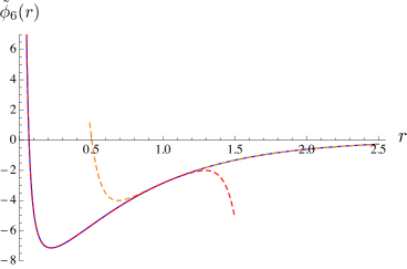
Figure 1: The solution for the mode $\tilde{\phi}_{6}$, for $X_{2}=0$, $X_{1}=X_{3}=X_{5}=X_{6}=1$, $X_{4}=10$, $Y_{a}=1$, $m=1$ (underlying blue solid line). The red and orange dashed curves correspond to the IR and UV expansions (respectively up to 20 and 15 terms).

3.2 Infrared expansions

We now show the IR expansions of the modes $\tilde{\phi}_{a}$, focusing on the singular behavior which is needed in order to impose boundary conditions in Section 5. These expansions appeared already in [13] and apart from making sure our results are fine in the present paper we relate $Y^{IR}$ to $Y^{UV}$, a crucial step in order to try and write the backreacted state at linearized order for all radii. Here the integration constants $X_{a}$ and $Y_{a}$ are those appearing in the analytic solution shown in section 2.1 and 2.2 and we defined the $\tilde{Y}_{a}$ as

$$\tilde{Y}_{a}=Y_{a}+\,m^{2}\,X_{4}\,k_{\tilde{\phi}_{a}}\,,$$ (3.6)

$$k_{\tilde{\phi}_{1}}=7.45479\,,\quad k_{\tilde{\phi}_{2}}=0.301287\,,\quad k_{\tilde{\phi}_{3}}=0.112188\,,\quad k_{\tilde{\phi}_{5}}=0.576358\,,\quad k_{\tilde{\phi}_{6}}=-0.00504419\,.$$

The constants $k_{\tilde{\phi}_{a}}$ are obtained with the numerical procedure outlined in the previous subsection. We also impose the zero energy condition (2.36) and so in what follows we set $X_{2}=0$. With these remarks and notations in mind, we now provide the IR expansions for the first–order perturbation modes

$$\tilde{\phi}_{1} =\frac{1}{4\,3^{3/4}r^{2}}\bigg{[}-27\,X_{1}-16\sqrt{3}\,(X_{5}+X_{6})-30\,m^{2}\,H_{0}\,X_{4}\bigg{]}$$ (3.7)

$$\quad+\frac{1}{12r}\bigg{[}6\tilde{Y}_{1}+\sqrt{2}\,3^{1/4}(-45\sqrt{3}\,X_{1}-162\sqrt{3}\,X_{3}+40\,X_{5}+112\,X_{6})K(-1)\bigg{]}$$

$$\quad+\frac{1}{12\cdot 3^{3/4}}\Big{(}189\,X_{1}-80\sqrt{3}\,(X_{5}+X_{6})+6\,m^{2}\,X_{4}(83\,H_{0}-3^{1/4}\,33)\Big{)}+\mathcal{O}(r)\,,$$

$$\tilde{\phi}_{2} =\frac{1}{r^{4}}\bigg{[}\frac{\tilde{Y}_{2}}{3}+\frac{4}{105}\,H_{0}\,(63\,X_{1}+432\,X_{3}-7\sqrt{3}\,(5\,X_{5}+11\,X_{6}))+\frac{63\,3^{1/4}}{5}\,X_{1}+\frac{2808}{35}\,3^{1/4}\,X_{3}$$

$$\quad-\frac{72}{5}\,3^{3/4}\,X_{6}\bigg{]}+\frac{1}{r^{2}}\bigg{[}-\frac{291}{20}\,3^{1/4}\,X_{1}-\frac{3744}{35}\,3^{1/4}\,X_{3}+2\,3^{3/4}\,X_{5}+\frac{106}{5}\,3^{3/4}\,X_{6}$$ (3.8)

$$\quad+H_{0}\,\Big{(}-\frac{16}{5}\,X_{1}-\frac{768\,X_{3}}{35}+\frac{3\,3^{1/4}\,m^{2}\,X_{4}}{2}+\frac{16\,(5\,X_{5}+11\,X_{6})}{15\sqrt{3}}\Big{)}-\frac{4\,\tilde{Y}_{2}}{9}\bigg{]}$$

$$\quad-\frac{1}{12r}\bigg{[}6\,\tilde{Y}_{1}-\sqrt{2}\,3^{1/4}(45\sqrt{3}\,X_{1}+162\sqrt{3}\,X_{3}-40\,X_{5}-112\,X_{6})K(-1)\bigg{]}$$

$$\quad+\frac{137\,3^{1/4}\,X_{1}}{25}+\frac{12792\,3^{1/4}\,X_{3}}{175}+6\sqrt{3}\,m^{2}\,X_{4}-\frac{1}{675}(225\,3^{3/4}\,X_{5}+9081\,3^{3/4}\,X_{6}-205\tilde{Y}_{2})$$

$$\quad+H_{0}\Big{(}\frac{164}{75}\,X_{1}+\frac{2624}{175}\,X_{3}-\frac{23\,3^{1/4}\,m^{2}\,X_{4}}{2}-\frac{164\,(5\,X_{5}+11\,X_{6})}{225\sqrt{3}}\Big{)}+\mathcal{O}(r)\,,$$

$$\tilde{\phi}_{3} =\frac{1}{r^{4}}\bigg{[}\frac{H_{0}}{70}\Big{(}-63\,X_{1}-432\,X_{3}+7\sqrt{3}(5\,X_{5}+11\,X_{6})\Big{)}-\frac{189\,3^{1/4}\,X_{1}}{40}-\frac{1053}{35}\,3^{1/4}\,X_{3}$$ (3.9)

$$\quad+\frac{27\,3^{3/4}\,X_{6}}{5}-\frac{\tilde{Y}_{2}}{8}\bigg{]}+\frac{1}{r^{2}}\bigg{[}\frac{2H_{0}}{105}\Big{(}63\,X_{1}+432\,X_{3}-7\sqrt{3}(5\,X_{5}+11\,X_{6})\Big{)}$$

$$\quad+\frac{237\,3^{1/4}\,X_{1}}{40}+\frac{1404\,3^{1/4}\,X_{3}}{35}-\frac{3^{3/4}}{10}(5\,X_{5}+77\,X_{6})+\frac{\tilde{Y}_{2}}{6}\bigg{]}$$

$$\quad+\frac{61}{160}3^{1/4}\,X_{1}-\frac{1167}{100}3^{1/4}\,X_{3}-\frac{67}{16}\sqrt{3}m^{2}\,X_{4}-\frac{671\,X_{5}-1033\,X_{6}}{120\,3^{1/4}}-\frac{41}{360}\,\tilde{Y}_{2}+\tilde{Y}_{3}$$

$$\quad+\frac{F_{0}}{630\sqrt{2}}\Big{(}-10836\,X_{1}-69444\,X_{3}+6300\,3^{1/4}\,m^{2}\,X_{4}+7\sqrt{3}\,(725\,X_{5}+1847\,X_{6})\Big{)}$$

$$\quad+\frac{K_{1}+K_{2}}{4\sqrt{2}}\Big{(}21\,X_{1}-4\sqrt{3}(X_{5}+X_{6})\Big{)}+30\sqrt{2}\,3^{1/4}\,m^{2}\,X_{4}\,F_{0}\log r$$

$$\quad+\frac{1}{8}\Big{(}21\,3^{1/4}\,X_{1}-210\,\sqrt{3}\,m^{2}\,X_{4}-4\,3^{3/4}\,(X_{5}+X_{6})\Big{)}\log r+\mathcal{O}(r)\,,$$

$$\tilde{\phi}_{5} =\frac{1}{5}\Big{(}-12\,3^{3/4}\,X_{1}-81\,3^{3/4}\,X_{3}+18\,3^{1/4}\,X_{6}+10\,\tilde{Y}_{6}\Big{)}$$ (3.10)

$$\quad-\frac{H_{0}}{60}\Big{(}21\sqrt{3}\,X_{1}+4\,(27\sqrt{3}\,X_{3}+10\,X_{5}+4\,X_{6})\Big{)}+\mathcal{O}(r^{3})\,,$$

$$\tilde{\phi}_{6} =\frac{H_{0}}{12\,r^{2}}\bigg{[}\sqrt{3}\,H_{0}\,m^{2}\,X_{4}-2\,(X_{5}+X_{6})\bigg{]}-H_{0}\,\Big{(}\frac{7\sqrt{3}\,X_{1}}{80}+\frac{9\sqrt{3}\,X_{3}}{20}+\frac{7\,m^{2}\,X_{4}}{24\,3^{1/4}}+\frac{10\,X_{5}+X_{6}}{90}\Big{)}$$

$$\quad-\frac{H_{0}^{2}\,m^{2}\,X_{4}}{12\sqrt{3}}-\frac{43\,3^{3/4}\,X_{1}}{80}-\frac{81\,3^{3/4}\,X_{3}}{20}+\frac{25\,X_{5}+106\,X_{6}}{30\,3^{3/4}}+\frac{\tilde{Y}_{6}}{2}+\mathcal{O}(r)\,,$$ (3.11)

$$\tilde{\phi}_{4} =\frac{1}{r^{2}}\Big{[}-\frac{3}{4}\,\,3^{1/4}\,H_{0}^{2}\,m^{2}\,X_{4}-\frac{1}{H_{0}}\Big{(}\frac{207\sqrt{3}\,X_{1}}{40}+\frac{2403\sqrt{3}\,X_{3}}{70}-\frac{54}{5}\,X_{6}+\frac{\tilde{Y}_{2}}{8\,3^{3/4}}-3^{3/4}\,\tilde{Y}_{6}\Big{)}$$

$$\quad-\frac{33}{40}\,3^{1/4}\,X_{4}-\frac{333}{70}\,3^{1/4}\,X_{3}-\frac{5\,X_{5}-X_{6}}{5\,3^{1/4}}\bigg{]}+\mathcal{O}(r^{0})\,.$$ (3.12)

3.3 Ultraviolet expansions

Here we show the leading terms in the UV expansions of the perturbation modes $\tilde{\phi}_{a}$

$$\tilde{\phi}_{1} =-\frac{27\,X_{3}}{2^{1/4}}e^{-r/2}+2e^{-2r}\,Y_{1}-e^{-5r/2}\,2^{7/4}\Big{(}27\,X_{1}+81\,X_{3}-16\sqrt{3}\,X_{6}\Big{)}$$ (3.13)

$$\quad+\frac{1}{20\,2^{1/4}}e^{-9r/2}\Big{(}3267\,X_{3}-1024\sqrt{3}\,X_{6}\Big{)}+\mathcal{O}(e^{-6r})\,,$$

$$\tilde{\phi}_{2} =-\frac{63\,X_{3}}{10\,2^{1/4}}e^{3r/2}-\frac{52569\,X_{3}}{280\,2^{1/4}}e^{-5r/2}-12e^{-4r}\,Y_{1}+\mathcal{O}(e^{-9r/2})\,,$$ (3.14)

$$\tilde{\phi}_{3} =Y_{3}-\frac{3Y_{1}}{8}+\frac{81\,X_{3}}{20\,2^{1/4}}e^{3r/2}-\frac{29079\,X_{3}}{560\,2^{1/4}}e^{-5r/2}+\frac{15}{4}e^{-4r}\,Y_{1}+\mathcal{O}(e^{-9r/2})\,,$$ (3.15)

$$\tilde{\phi}_{5} =\frac{Y_{5}-Y_{6}}{8}e^{3r}-\frac{9\,(Y_{5}-Y_{6})}{8}e^{r}+\frac{1}{24}e^{-r}\Big{(}-8\sqrt{3}\,Y_{1}+117\,Y_{5}+27\,Y_{6}\Big{)}$$ (3.16)

$$\quad-38\,2^{3/4}\sqrt{3}e^{-3r/2}\,X_{3}+\frac{1}{72}e^{-3r}\Big{(}168\sqrt{3}Y_{1}-9\,(111\,Y_{5}+Y_{6})\Big{)}$$

$$\quad+\frac{2}{195}2^{3/4}e^{-7r/2}(-3348\sqrt{3}X_{1}+1323\sqrt{3}X_{3}+6160\,X_{6})+\mathcal{O}(e^{-5r})\,,$$

$$\tilde{\phi}_{6} =-\frac{Y_{5}-Y_{6}}{16}e^{3r}-\frac{3\,(Y_{5}-Y_{6})}{16}e^{r}+\frac{1}{144}e^{-r}\Big{(}-8\sqrt{3}\,Y_{1}+117\,Y_{5}+27\,Y_{6}\Big{)}$$ (3.17)

$$\quad-5\,2^{3/4}\sqrt{3}\,e^{-3r/2}\,X_{3}+\frac{1}{48}e^{-3r}\Big{(}8\sqrt{3}Y_{1}-51\,Y_{5}+3\,Y_{6})\Big{)}$$

$$\quad+\frac{1}{585}2^{3/4}e^{-7r/2}\Big{(}-1188\sqrt{3}X_{1}+243\sqrt{3}X_{3}+2320\,X_{6})+\mathcal{O}(e^{-5r})\,,$$

$$\tilde{\phi}_{4} =\frac{3\,Y_{4}^{UV}}{16\,2^{3/4}m^{2}}\,e^{9r/2}+\frac{27\,Y_{4}^{UV}}{26\,2^{3/4}\,m^{2}}\,e^{5r/2}-\frac{27\,X_{3}}{10\,2^{1/4}}\,e^{3r/2}+\frac{350271\,Y_{4}^{UV}}{182872\,2^{3/4}\,m^{2}}\,e^{r/2}$$ (3.18)

$$\quad+\frac{3\,Y_{1}}{2}-2\,Y_{3}-2\sqrt{3}\,Y_{5}+2\sqrt{Y_{6}}-\frac{324}{325}\,2^{3/4}\,X_{3}\,e^{-r/2}+\frac{484605\,Y_{4}^{UV}}{298792\,2^{3/4}\,m^{2}}\,e^{-3r/2}$$

$$\quad-\frac{24}{13}(Y_{1}-6\sqrt{3}\,Y_{6})\,e^{-2r}-\frac{11957859009\,X_{3}}{28155400\,2^{1/4}}\,e^{-5r/2}+\frac{7978373883\,Y_{4}^{UV}}{21130570240\,2^{3/4}\,m^{2}}\,e^{-7r/2}+\mathcal{O}(e^{-4r})\,.$$

From these expansions we can extract the UV behavior of the fields $\tilde{\phi}_{a}$, which is important to understand the holographic physics. For this purpose we have to relate our radial variable $r$ to the standard $AdS$ coordinate $\rho_{AdS}$ as

$$\rho_{AdS}\sim e^{3r/2}\,.$$ (3.19)

A discussion of the holographic behavior can be found in [13], where it was shown that the integration constants $X_{a}$ and $Y_{a}$ are paired into normalizable and non-normalizable mode. In order to be self–contained we tabulate in Table 1 (which is adapted from [13]), the leading terms coming from each modes. Note that since we obtain the asymptotic behavior from an analytic solution, we can relate the integration constants of [13] to the IR singular behavior of the same modes. In particular, one can explicitly check if an IR regularity condition on one integration constant is compatible with the absence of the respective non–normalizable mode in the UV. We will come back on this point in the next section. In the following table $\Delta$ is the dimension of the local operator $\mathcal{O}$ holographically associated to the two supergravity modes whose asymptotic is $\rho_{AdS}^{-\Delta}$ (dual to the vacuum expectation value of $\mathcal{O}$) and $\rho_{AdS}^{\Delta-3}$ (dual to a deformation of the action $\delta S=\int d^{3}x\,\mathcal{O}$). Also, the combination which appears at dimension $\Delta=7/3$ is the linear combination of $Y_{1}$, $Y_{5}$ and $Y_{6}$ which appears in the corresponding terms in (3.16) and (3.17).

dim $\Delta$	non-norm/norm	integration constants
6	$\rho_{AdS}^{3}/\rho_{AdS}^{-6}$	$Y_{4}/X_{4}$
5	$\rho_{AdS}^{2}/\rho_{AdS}^{-5}$	$Y_{5}-Y_{6}/X_{5}-X_{6}$
4	$\rho_{AdS}/\rho_{AdS}^{-4}$	$X_{3}/Y_{2}$
3	$\rho_{AdS}^{0}/\rho_{AdS}^{-3}$	$Y_{1}+Y_{3}/X_{2}$
$\frac{7}{3}$	$\rho_{AdS}^{-2/3}/\rho_{AdS}^{-7/3}$	$Y_{5}+Y_{6}+Y_{1}/X_{5}+X_{6}$
$\frac{5}{3}$	$\rho_{AdS}^{-4/3}/\rho_{AdS}^{-5/3}$	$Y_{1}/X_{1}$

Table 1: The UV behavior of all fourteen modes for the $SO(5)$-symmetric deformation around the CGLP solution, extracted from the asymptotic of our analytic solution.

4 Charges and M2–branes

The space of solutions we solved for in the previous sections should contain the linearized perturbation of the warped Stenzel space due to the presence of a stack of smeared anti–M2 branes placed at the tip of the geometry. This configuration was studied in the probe approximation in [10] and corresponds in the dual gauge theory to a metastable supersymmetry breaking state. In order to identify the backreacted solution, we need to impose the correct boundary conditions associated to the presence of the anti–branes at the tip. In this section we start by discussing the standard notions of charge in the Stenzel background (see for example [20, 21, 22]) and as a warmup we identify the BPS perturbation of the CGLP solution ascribed to the presence of M2 branes. The anti–M2 brane perturbation will be discussed in the next section.

In the Stenzel background we can define a “running” M2 charge by integrating $\star_{11}G_{4}$ on a 7–dimensional section $\mathcal{M}_{r}=V_{5,2}$ of the transverse cone at a fixed $r$

$$Q_{M2}(r)=\frac{1}{(2\pi l_{p})^{6}}\int_{\mathcal{M}_{r}}\star_{11}G_{4}\,,$$ (4.1)

where $l_{p}$ is the Planck length in eleven dimensions. We can also integrate $G_{4}$ over the 4–sphere which has a finite size at the tip and define the quantity

$$q(r)=\frac{1}{(2\pi l_{p})^{3}}\int_{S_{4}}G_{4}\,.$$ (4.2)

For the parametrization (2.1)-(2.2) and for the CGLP background we find from (2.33) (see also Appendix B)

$$Q_{M2}^{0}(r) =-\frac{6\,2^{11}\,m^{2}\,\text{Vol}_{V_{5,2}}}{3^{4}\,(2\pi l_{p})^{6}}\Big{(}h_{0}(f_{0}-2h_{0})-\frac{1}{54}\Big{)}\,,$$ (4.3)

$$q^{0}(r) =-\frac{16\pi^{2}m}{(2\pi l_{p})^{3}}h_{0}(r)\,,$$ (4.4)

where $\text{Vol}_{V_{5,2}}=27\pi^{4}/128$ [23]. Substituting the zeroth–order solution (2.15) we find

$$Q_{M2}^{0}(r)=\frac{\,m^{2}\,\tanh^{4}r}{108\,\pi^{2}\,l_{p}^{6}}\,,\quad q^{0}(r)=\frac{m\,{\rm sech\,}r}{3\sqrt{3}\,\pi\,l_{p}^{3}}\,,$$ (4.5)

which is the known result for the CGLP solution [10].

We now want to calculate the first–order corrections to these charges from the first–order perturbation of the Stenzel geometry. The simpler case is the BPS one, where a stack of M2–branes smeared over the $S^{4}$ is placed at the origin $r=0$. The perturbation on the geometry should still preserve supersymmetry, so we are forced to set $X_{a}=0$, $a=1,\dots,6$ since the “conjugate–momenta” $\tilde{\xi}_{a}$ are the modes that parametrize the supersymmetry breaking. Note that in this case the solutions for the modes $\tilde{\phi}_{a}$ are given by the homogenous solutions of the coupled system of ODE’s (2.27)–(2.32) and they are easily found by setting $\tilde{\xi}_{a}=0$ in (2.39). The perturbation due to the presence of M2 branes at the tip is found by imposing the following conditions on the $Y_{a}$ integration constants: $Y_{1}=Y_{2}=0$ to cancel IR divergencies in $\tilde{\phi}_{1}$ and $\tilde{\phi}_{2}$, $Y_{4}=Y_{5}-Y_{6}=0$ to cancel the divergent terms in the UV expansions of $\tilde{\phi}_{4}$ and $\tilde{\phi}_{5}$, and finally $Y_{3}=0$ to fix the freedom of rescaling the three–dimensional coordinates. The first–order perturbation to (4.3) is proportional to $h_{0}(\tilde{\phi}_{5}-4\tilde{\phi}_{6})+f_{0}\tilde{\phi}_{6}$ and at the linearized level the running M2 charge is given by

$$Q_{M2}=Q_{M2}^{0}+Q_{M2}^{1}=\frac{m^{2}\,l_{p}^{-6}}{108\,\pi^{2}}\bigg{[}\tanh^{4}r+6\sqrt{3}\,Y_{6}\Big{(}1-\tanh^{4}r\Big{)}\bigg{]}\,.$$ (4.6)

The profile of the charge is shown in Figure 2 for different values of the constant $Y_{6}$.

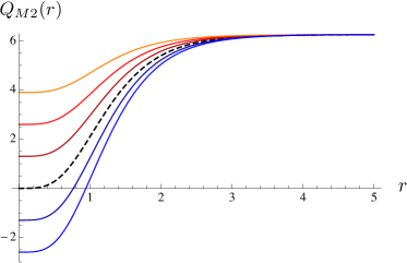
Figure 2: The profile of the M2 charge $Q_{M2}$ for the BPS perturbation, for different values of the parameter $Y_{6}$. The black dashed line is the zeroth–order solution ($Y_{6}=0$). Note that at the linearized level the perturbations vanish in the UV.

The asymptotic behavior is the following

$$Q_{M2}^{IR}=\frac{m^{2}\,l_{p}^{-6}}{6\sqrt{3}\,\pi^{2}}\,Y_{6}+\mathcal{O}(r^{4})\,,\qquad Q_{M2}^{UV}=\frac{m^{2}\,l_{p}^{-6}}{108\,\pi^{2}}+\mathcal{O}(e^{-2r})\,.$$ (4.7)

The integral of $G_{4}$ over the four–sphere is given by the behavior of the mode $h\sim\tilde{\phi}_{6}$ and thus

$$q=q^{0}+q^{1}=\frac{m\,l_{p}^{-3}}{3\sqrt{3}\pi}\Big{(}1-3\sqrt{3}\,Y_{6}\Big{)}\,{\rm sech\,}r\,.$$ (4.8)

We see that $q$ vanishes at infinity while in the IR it approaches a constant value

$$q^{IR}=\frac{m\,l_{p}^{-3}}{3\sqrt{3}\pi}\Big{(}1-3\sqrt{3}\,Y_{6}\Big{)}+\mathcal{O}(r^{2})\,,\qquad q^{UV}=\mathcal{O}(e^{-r})\,.$$ (4.9)

We will denote $\tilde{M}=q^{0}(0)$ the number of $G_{4}$ flux units through the non–vanishing $S^{4}$ at the tip. Note that for the zeroth-order solution we have

$$\frac{(\tilde{M})^{2}}{4}=Q_{M2}^{UV}\,.$$ (4.10)

At first–order, we expect a term related to the explicit brane charge in the IR; in fact, we easily see from (4.9) that our solution satisfies

$$\frac{(q^{IR})^{2}}{4}=Q_{M2}^{UV}-Q_{M2}^{IR}\,,$$ (4.11)

which indeed reduces to (4.10) when $Y_{6}=0$, which corresponds to having no regular M2–branes. Allowing a nonzero $Y_{6}$ introduces a singularity in the warp factor $\tilde{\phi}_{4}$

$$\tilde{\phi}_{4}=\frac{3^{3/4}\,Y_{6}}{H_{0}\,r^{2}}+\mathcal{O}(r^{0})\,,$$ (4.12)

which is the expected divergency due to smeared M2 branes on the $S^{4}$ at the tip.

We could have derived these results without relying on the actual solution for the $\tilde{\phi}_{a}$ modes. In fact, the linearized BPS perturbation can be obtained by simply shifting the fluxes as follows [13]

$$\tilde{\phi}_{5} =2c\,,$$ (4.13)

$$\tilde{\phi}_{6} =\frac{c}{2}\,,$$

where $c$ is the number of M2 branes. The M2 charge thus changes in the following way

$$Q_{M2}^{(1)}=-\frac{m^{2}\,l_{p}^{-6}}{2\,\pi^{2}}\left(h_{0}(\tilde{\phi}_{5}-4\tilde{\phi}_{6})+f_{0}\tilde{\phi}_{6}\right)=-\frac{c\,m^{2}\,l_{p}^{-6}}{4\,\pi^{2}}\,f_{0}=\frac{c\,m^{2}\,l_{p}^{-6}}{6\sqrt{3}\,\pi^{2}}+\mathcal{O}(r^{4})\,,$$ (4.14)

while for the warp factor we have, from (2.32)

$$\Delta\tilde{\phi}_{4}^{\prime}=c\,m^{2}f_{0}(r)\,e^{-3(z_{0}+\alpha_{0}+\beta_{0})}\overset{r\rightarrow 0}{\sim}-\frac{2\,3^{3/4}\,c}{H_{0}\,r^{3}}\,,$$ (4.15)

from which we get

$$\tilde{\phi}_{4}=\frac{3^{3/4}\,c}{H_{0}\,r^{2}}+\mathcal{O}(r^{0})\,,$$ (4.16)

which agrees with (4.12) with the identification $Y_{6}=c$. From this result we can also extract the correct mass/charge normalization between the warp factor divergency and the charge sourced by the branes, which will be useful in the next section

$$m^{2}\,H_{0}\,r^{2}\,\tilde{\phi}_{4}=18\cdot 3^{1/4}\,\pi^{2}\,l_{p}^{6}\,|Q_{M2}^{IR}|\,.$$ (4.17)

In the next section, we will turn to the case of interest in which we add a stack of anti–M2 branes at the tip of the transverse Stenzel space. In this case the expressions (4.3), (4.4) evaluated at first–order in perturbation theory will depend on all of the $X_{a},Y_{a}$ integration constants. However, we have to impose appropriate regularity conditions for the IR and UV behavior of the modes $\tilde{\phi}_{a}$, and we will see that this fixes all the integration constants in terms of $X_{4}$, which is the one responsible for the force on a probe M2 brane in this background (see section 5.3), and $Y_{6}$. We thus expect the expressions for the charges in the BPS case to be modified by some pieces proportional to $X_{4}$. By requiring the variation in the M2 charge $Q_{M2}^{(1)}$ to be commensurate to the singularity introduced in the warp factor, equation (4.17), we will derive a relation which fixes $Y_{6}$ in terms of $X_{4}$ and so we will fix all the integration constants in terms of the number of anti–M2 branes.

5 The anti–M2 brane perturbation

In this section we consider the perturbed solution corresponding to a stack of $\bar{N}$ anti–M2 branes at the tip of the transverse geometry. It was shown in [10] that in the probe approximation, for $\bar{N}/\tilde{M}\lesssim 0.054$ this configuration is metastable and will eventually decay into a supersymmetric configuration in which $\tilde{M}-1-\bar{N}$ M2 branes are present at the tip . In order to find the supergravity dual to the metastable state, we will adopt the following strategy. Firstly, we consider the IR behavior and we allow only for divergencies that are directly sourced by the anti-branes. Secondly, we demand that the UV non-normalizable modes described in section 3.3 are absent, so that the UV asymptotic is the same as for the original CGLP background. As we will show, these requirements (together with the mass/charge normalization discussed in the previous section) provide enough independent contraints on the deformation space to fix every integration constants in terms of a single physical quantity, namely the number of anti–M2 branes present at the tip. We then compute the relevant charges for the perturbed solution, as well as the explicit expression for the force felt by probe M2 branes in the backreacted anti–M2 background.

5.1 IR and UV boundary conditions

We now proceed to impose regularity conditions on the IR behavior of the modes $\tilde{\phi}_{a}$. We demand that divergencies are zero except for the singularity in the warp factor $\tilde{\phi}_{4}$ which is directly sourced by the anti–M2 branes. We first impose the zero energy condition, which amounts to setting

$$X_{2}=0\,.$$ (5.1)

From regularity of $\tilde{\phi}_{1}$ we derive

$$X_{1} =-\frac{2}{27}\bigg{[}8\sqrt{3}(X_{5}+X_{6})+15\,m^{2}\,X_{4}\,H_{0}\bigg{]}\,,$$ (5.2)

$$X_{5} =\frac{27\sqrt{3}\,X_{3}}{20}-\frac{8\,X_{6}}{5}-\frac{Y_{1}}{20\sqrt{2}\,3^{1/4}K(-1)}-\frac{m^{2}\,X_{4}\,\big{(}100\,H_{0}\,K(-1)+\sqrt{2}\,3^{1/4}k_{\tilde{\phi}_{1}}\big{)}}{80\sqrt{3}\,K(-1)}\,,$$

while from the singular terms in $\tilde{\phi}_{2}$ we derive $X_{6}$ and $Y_{2}$ in terms of $X_{3}$, $X_{4}$ and $Y_{1}$

$$X_{6} =\frac{9\sqrt{3}\,X_{3}}{4}-\frac{Y_{1}}{12\sqrt{2}\,3^{1/4}K(-1)}-\frac{m^{2}\,X_{4}\,\big{(}220\,H_{0}\,K(-1)+\sqrt{2}\,3^{1/4}k_{\tilde{\phi}_{1}}\big{)}}{48\sqrt{3}\,K(-1)}\,,$$ (5.3)

$$Y_{2} =\frac{594}{35}\,(3\,3^{1/4}-H_{0})\,X_{3}-\frac{\sqrt{2}3^{1/4}(9\,3^{1/4}+H_{0})\,Y_{1}}{5\,K(-1)}-\frac{m^{2}\,X_{4}}{10\,K(-1)}\Big{[}\sqrt{2}3^{1/4}(9\,3^{1/4}+H_{0})k_{\tilde{\phi}_{1}}$$

$$\quad+30K(-1)k_{\tilde{\phi}_{2}}+8H_{0}(153\,3^{1/4}+2H_{0})K(-1)\Big{]}\,.$$

We can check that with these conditions the other IR divergencies of the modes $\tilde{\phi}_{a}$ are automatically canceled, except for a $\log r$ mode in the IR behavior of the field $\tilde{\phi}_{3}$, which is a perturbation of the metric, which is proportional to $X_{4}$. It is not clear why one should not be able to kill such divergent behavior. However, after imposing the previous boundary conditions, the solution presents an even worse singularity appearing in the field strength $F_{4}^{2}$ [13]

$$F_{4}^{2}\sim\frac{X_{4}^{2}}{r^{4}}\,,$$ (5.4)

which is quite analogous to the divergence found in the anti–D3 solution [7], with the difference that now the action is divergent. This behavior is sub–leading with respect to the energy density associated to the divergency in the warp factor, which is of order $r^{-6}$. Note that this is an IR phenomenon insensible to UV boundary conditions; in fact, the integration constant $X_{4}$ cannot be set to zero for the very simple reason that it parametrizes the force felt by a probe M2 brane [13] and thus is indicative of the presence of anti–M2 branes at the tip. Despite arguments in the literature, there is not a rigorous proof that shows if this singularity is acceptable or not. Given the difficulties in proving this, we will assume that the singularity is harmless and we will try to see if the anti–M2 solution develops problems in the UV; if this is not the case, the solution we find describes the holographic dual of the conjectured metastable state in the field theory, but clearly a more detailed study of the IR singularity is required to decide whether this supergravity solution can be trusted or not.

We now proceed by imposing boundary conditions in the UV, where we demand that non–normalizable modes in the UV expansions for the modes $\tilde{\phi}_{a}$ are absent. The first condition is from the $e^{3r/2}$ term in $\tilde{\phi}_{2}$, from which we get

$$X_{3}=0\,.$$ (5.5)

From the divergent term in $\tilde{\phi}_{5}$ we get

$$Y_{5}=Y_{6}\,,$$ (5.6)

and finally from the term $e^{-2r}$ in $\tilde{\phi}_{1}$ we get

$$Y_{1}=0\,.$$ (5.7)

Note that we should allow an $e^{-r}$ term in the fluxes, which is dual to the dimension $\Delta=7/3$ operator, since it is the charge mode sourced by the branes. We thus see that we fixed the ten physically relevant integration constants in terms of $X_{4}$ and $Y_{6}$, which are related respectively to the force on a probe M2 brane and to the number $\bar{N}$ of anti–M2 branes placed at the tip [13].

5.2 Charges and anti–M2 branes

In order to relate $X_{4}$ and $Y_{6}$ we look at the M2 charge (4.1). Once all the boundary conditions are imposed, we get that

$$Q_{M2}^{IR}=\frac{m^{2}\,\tilde{\phi}_{5}(0)}{12\sqrt{3}\,\pi^{2}\,l_{p}^{6}}=\frac{m^{2}}{6\sqrt{3}\,\pi^{2}\,l_{p}^{6}}\,(Y_{6}-\alpha\,m^{2}\,X_{4})\,,$$ (5.8)

where the coefficient $\alpha$ is the following combination of the numerical constants which enters in the expansions for the modes $\tilde{\phi}_{a}$

$$\alpha=\frac{H_{0}(63\,3^{1/4}+22H_{0})}{60\sqrt{3}}-k_{\tilde{\phi}_{6}}+\frac{(27+3^{3/4}\,H_{0})\,k_{\tilde{\phi}_{1}}}{360\,\sqrt{2}K(-1)}\sim 0.900178\,.$$ (5.9)

We impose that this variation gives the correct singularity in the infrared expansion for the warp factor, which is found to be

$$\tilde{\phi}_{4}=\frac{3^{3/4}\,(Y_{6}-\beta\,m^{2}\,X_{4})}{H_{0}\,r^{2}}+\mathcal{O}(r^{0})\,,$$ (5.10)

with

$$\beta=\alpha+\frac{H_{0}^{2}}{\sqrt{3}}\sim 0.958828\,.$$ (5.11)

From the mass/charge normalization (4.17) we thus get the following condition

$$-Y_{6}+\alpha\,m^{2}\,X_{4}=Y_{6}-\beta\,m^{2}\,X_{4}\,,$$ (5.12)

which results in

$$Y_{6}=\frac{1}{2}(\alpha+\beta)\,m^{2}\,X_{4}=\Big{(}\alpha+\frac{H_{0}^{2}}{2\sqrt{3}}\Big{)}\,m^{2}\,X_{4}\,.$$ (5.13)

If we now plug this relation back into the expression for the charge (5.8), we find the following relation

$$Q_{M2}^{IR}=-\bar{N}=\frac{H_{0}^{2}\,m^{4}\,X_{4}}{36\,\pi^{2}\,l_{p}^{6}}\,.$$ (5.14)

We note that this result does not depend on the UV boundary conditions. Indeed, although it is not clear from our derivation, it is easy to show that if we only impose IR boundary conditions the terms proportional to $X_{3},Y_{5}$ and $Y_{1}$ that appear in (5.8) and (5.10) cancel in (5.13).

Since $Q_{M2}^{IR}$ is related to the number $\bar{N}$ of anti–M2 branes placed at the tip, from (5.14) we determine $X_{4}$ as a function of $\bar{N}$ and thus we fix all the integration constants in terms of this parameter.

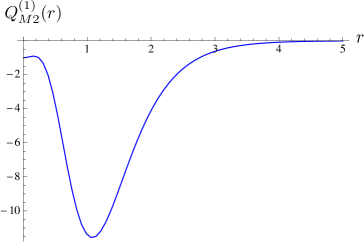
Figure 3: The profile of the first–order M2 charge $Q_{M2}^{(1)}$ for the anti–M2 solution, setting $\bar{N}=1$.

With these results, we can explicitly compute the charges associated to the anti–M2 brane perturbation (in Figure 3 we show the profile of the first–order perturbation to the Maxwell charge $Q_{M2}^{(1)}$). In particular, the M2 charge $Q_{M2}$ evaluated at a holographic screen at infinity should be the same for the metastable and the supersymmetric state. This condition ensures that the metastable state is a state in the same theory which is dual to the supersymmetric vacuum. Unfortunately, we see from (4.7) that the perturbation to the M2 charge vanishes at infinity at the linearized level, and so in our backreacted solution the value of $Q_{M2}^{UV}$ is fixed. We expect shifts of this quantity to appear only at second–order in perturbation theory. While we cannot directly check whether the value of the charge at infinity is conserved, we can look in the IR and check whether the charges are perturbed in a consistent way. From the probe computation (see footnote 8), we expect relation (4.11) to be satisfied. For a supersymmetric domain wall, this easily follows from the equation of motion (2.4) and the self–duality of the flux $G_{4}$, and indeed we found that the BPS perturbation considered in section 4 is consistent with this constraint at the linearized level. For the non–supersymmetric case, one should be more careful. It is useful to write the first–order perturbation to the Maxwell charge in the IR in the following way

$$Q_{M2}^{IR}=\frac{m^{2}\,l_{p}^{-6}}{2\pi^{2}}\bigg{[}\frac{1}{6\sqrt{3}}\left(\tilde{\phi}_{5}(0)-4\,\tilde{\phi}_{6}(0)\right)+\frac{2}{3\sqrt{3}}\tilde{\phi}_{6}(0)\bigg{]}\,,$$ (5.15)

from which we derive, at the linearized level

$$\frac{(q_{IR})^{2}}{4}=\frac{m^{2}\,l_{p}^{-6}}{\pi^{2}}\Big{[}-\frac{1}{6\sqrt{3}}+\tilde{\phi}_{6}(0)\Big{]}^{2}=Q_{M2}^{UV}-Q_{M2}^{IR}+\frac{m^{2}\,l_{p}^{-6}}{12\sqrt{3}\pi^{2}}\Big{[}\tilde{\phi}_{5}(0)-4\,\tilde{\phi}_{6}(0)\Big{]}+\mathcal{O}(X^{2})\,.$$ (5.16)

After imposing the anti–M2 IR boundary conditions, we find that the term in the brakets in the right hand side of the last equation is not zero

$$\tilde{\phi}_{5}(0)-4\,\tilde{\phi}_{6}(0)=H_{0}\,3^{-1/4}\,m^{2}\,X_{4}\,.$$ (5.17)

Indeed, this is the term which gives rise to the singularity in the filed strength $F_{4}^{2}$ that we discussed in section 5.1. This result is consistent with the fact that at the linearized level the self–duality of the four–form flux is spoiled, and we do not expect relation (4.11) to be satisfied for the anti–M2 solution. As we discussed in the previous subsection, it is possible that this result is an artifact of the perturbation theory. While we cannot address this issue within our first–order technology, we believe that further investigation is needed on this problem.

5.3 The force on a probe brane

With the results obtained in the previous subsections, we are able to compute explicitly the coefficient of the force exerted on a probe M2–brane in the anti–M2 backreacted background, whose functional form has been derived in [13, 18]:

$$F_{M2}=-\frac{18\,X_{4}\,{\rm csch\,}^{3}r}{(2+\cosh 2r)^{3/4}}\,.$$ (5.18)

Inserting the expression for $X_{4}$ that we derive from (5.14) we obtain

$$F_{M2}=\frac{648\,\pi^{2}\,l_{p}^{6}\,\bar{N}\,{\rm csch\,}^{3}r}{m^{4}\,H_{0}^{2}\,(2+\cosh 2r)^{3/4}}\,.$$ (5.19)

This result has to be compared to the one given by the probe anti–brane potential à la KKLMMT [28], which is given in [18] and reviewed in Appendix B. The result of this computation is given in (B). Once we substitute $d_{2}$ we see that the two expressions exactly agree. This is a nontrivial check that our IR boundary conditions are the correct ones to describe anti–M2 branes in the Stenzel geometry.

5.4 Asymptotic of the anti–M2 solution

We now collect the results we obtained for the twelve $(X_{a},Y_{a})$ integration constants and which determine the anti–M2 solution in terms of the constant $X_{4}$, which is fixed in terms of $\bar{N}$ by (5.14)

$$X_{4}=-\frac{36\,\pi^{2}\,l_{p}^{6}}{m^{4}\,H_{0}^{2}}\,\bar{N}\,.$$ (5.20)

For the $X_{a}$ integration constants we have

$$X_{1} =-2\,H_{0}\,m^{2}\,X_{4}\,,\quad X_{2}=0\,,\quad X_{3}=0\,,$$ (5.21)

$$X_{5} =\bigg{[}73\,H_{0}+2\,3^{1/4}\sqrt{\pi}\,k_{\tilde{\phi}_{1}}\,\Gamma\left(\frac{1}{4}\right)^{-2}\bigg{]}\,\frac{m^{2}\,X_{4}}{12\sqrt{3}}\,,$$

$$X_{6} =\bigg{[}-55\,H_{0}-2\,3^{1/4}\sqrt{\pi}\,k_{\tilde{\phi}_{1}}\,\Gamma\left(\frac{1}{4}\right)^{-2}\bigg{]}\,\frac{m^{2}\,X_{4}}{12\sqrt{3}}\,,$$

For the $Y_{a}$ integration constants we have

$$Y_{1} =0\,,$$ (5.22)

$$Y_{2} =\bigg{[}-\frac{4}{5}\,H_{0}(153\,3^{1/4}+2\,H_{0})-3\,k_{\tilde{\phi}_{2}}-\frac{4}{5}\,3^{1/4}(9\,3^{1/4}+H_{0})\sqrt{\pi}\,\Gamma\left(\frac{1}{4}\right)^{-2}\bigg{]}\,m^{2}\,X_{4}\,,$$

$$Y_{3} =0\,,$$

$$Y_{5} =Y_{6}=\bigg{[}\sqrt{3}\,H_{0}(63\,3^{1/4}+52\,H_{0})-180\,k_{\tilde{\phi}_{6}}+2\,(27+3^{3/4}\,H_{0})\sqrt{\pi}\,k_{\tilde{\phi}_{1}}\,\Gamma\left(\frac{1}{4}\right)^{-2}\bigg{]}\frac{m^{2}\,X_{4}}{180}\,.$$

The IR and UV behavior of the backreacted anti–M2 solution, up to the desired order, can be read off from the analytic solution presented in Appendix A after imposing the boundary conditions (5.21), (5.22). For the reader’s convenience, we show here the first few terms of the ultraviolet behavior of the solution.

$$\tilde{\phi}_{1} =\frac{4\,m^{2}\,X_{4}}{3K(-1)}\,\bigg{[}29\,2^{3/4}\,H_{0}\,K(-1)+6^{1/4}\,k_{\tilde{\phi}_{1}}\bigg{]}\,e^{-5r/2}$$ (5.23)

$$\quad+\frac{16\,m^{2}\,X_{4}}{15K(-1)}\bigg{[}110\,2^{3/4}\,H_{0}\,K(-1)+6^{1/4}\,k_{\tilde{\phi}_{1}}\bigg{]}\,e^{-9r/2}$$

$$\quad+\frac{7\,m^{2}\,X_{4}}{3K(-1)}\,\bigg{[}29\,2^{3/4}\,H_{0}\,K(-1)+6^{1/4}\,k_{\tilde{\phi}_{1}}\bigg{]}\,e^{-13r/2}+\mathcal{O}(e^{-17r/2})\,,$$

$$\tilde{\phi}_{2} =\frac{8\,m^{2}\,X_{4}}{3K(-1)}\,\bigg{[}143\,2^{3/4}\,H_{0}\,K(-1)+4\,6^{1/4}\,k_{\tilde{\phi}_{1}}\bigg{]}\,e^{-9r/2}$$ (5.24)

$$\quad-\frac{16\,m^{2}\,X_{4}}{5K(-1)}\bigg{[}8\,H_{0}\,(153\,3^{1/4}+2\,H_{0})\,K(-1)+\sqrt{2}\,3^{1/4}(9\,3^{1/4}+H_{0})\,k_{\tilde{\phi}_{1}}+30\,K(-1)\,k_{\tilde{\phi}_{2}}\bigg{]}\,e^{-6r}$$

$$\quad+\,m^{2}\,X_{4}\,\bigg{[}2816\,2^{3/4}\,H_{0}+\frac{128\,6^{1/4}\,k_{\tilde{\phi}_{1}}}{5K(-1)}\bigg{]}\,e^{-13r/2}+\mathcal{O}(e^{-17r/2})\,,$$

$$\tilde{\phi}_{3} =-\frac{4\,m^{2}\,X_{4}}{9K(-1)}\,\bigg{[}295\,2^{3/4}\,H_{0}\,K(-1)+8\,6^{1/4}\,k_{\tilde{\phi}_{1}}\bigg{]}\,e^{-9r/2}$$ (5.25)

$$\quad+\frac{6\,m^{2}\,X_{4}}{5K(-1)}\bigg{[}8\,H_{0}\,(153\,3^{1/4}+2\,H_{0})\,K(-1)+\sqrt{2}\,3^{1/4}(9\,3^{1/4}+H_{0})\,k_{\tilde{\phi}_{1}}+30\,K(-1)\,k_{\tilde{\phi}_{2}}\bigg{]}\,e^{-6r}$$

$$\quad-\,m^{2}\,X_{4}\,\bigg{[}\frac{14080}{13}\,2^{3/4}\,H_{0}+\frac{128\,6^{1/4}\,k_{\tilde{\phi}_{1}}}{13K(-1)}\bigg{]}\,e^{-13r/2}+\mathcal{O}(e^{-17r/2})\,,$$

$$\tilde{\phi}_{5} =\frac{m^{2}\,X_{4}}{30}\bigg{[}\sqrt{3}\,H_{0}(63\,3^{1/4}+52\,H_{0})-180\,k_{\tilde{\phi}_{6}}+2\,(27+3^{3/4}\,H_{0})\sqrt{\pi}\,k_{\tilde{\phi}_{1}}\,\Gamma\left(\frac{1}{4}\right)^{-2}\bigg{]}\,e^{-r}$$ (5.26)

$$\quad-\frac{7\,m^{2}\,X_{4}}{90}\bigg{[}\sqrt{3}\,H_{0}(63\,3^{1/4}+52\,H_{0})-180\,k_{\tilde{\phi}_{6}}+2\,(27+3^{3/4}\,H_{0})\sqrt{\pi}\,k_{\tilde{\phi}_{1}}\,\Gamma\left(\frac{1}{4}\right)^{-2}\bigg{]}\,e^{-3r}$$

$$\quad-m^{2}\,X_{4}\,\bigg{[}\frac{48872\,2^{3/4}\,H_{0}}{585\sqrt{3}}+\frac{308\,2^{1/4}\,k_{\tilde{\phi}_{1}}}{117\,3^{1/4}\,K(-1)}\bigg{]}\,e^{-7r/2}$$

$$\quad+\frac{m^{2}\,X_{4}}{6}\bigg{[}\sqrt{3}\,H_{0}(63\,3^{1/4}+52\,H_{0})-180\,k_{\tilde{\phi}_{6}}+2\,(27+3^{3/4}\,H_{0})\sqrt{\pi}\,k_{\tilde{\phi}_{1}}\,\Gamma\left(\frac{1}{4}\right)^{-2}\bigg{]}\,e^{-5r}$$

$$\quad+m^{2}X4\bigg{[}\frac{301448\,2^{3/4}\,H_{0}}{585\sqrt{3}}+\frac{131012\,2^{1/4}\,k_{\tilde{\phi}_{1}}}{9945\,3^{1/4}\,K(-1)}\bigg{]}\,e^{-11r/2}+\mathcal{O}(e^{-7r})\,,$$

$$\tilde{\phi}_{6} =\frac{m^{2}\,X_{4}}{180}\bigg{[}\sqrt{3}\,H_{0}(63\,3^{1/4}+52\,H_{0})-180\,k_{\tilde{\phi}_{6}}+2\,(27+3^{3/4}\,H_{0})\sqrt{\pi}\,k_{\tilde{\phi}_{1}}\,\Gamma\left(\frac{1}{4}\right)^{-2}\bigg{]}\,e^{-r}$$ (5.27)

$$\quad-\frac{\,m^{2}\,X_{4}}{180}\bigg{[}\sqrt{3}\,H_{0}(63\,3^{1/4}+52\,H_{0})-180\,k_{\tilde{\phi}_{6}}+2\,(27+3^{3/4}\,H_{0})\sqrt{\pi}\,k_{\tilde{\phi}_{1}}\,\Gamma\left(\frac{1}{4}\right)^{-2}\bigg{]}\,e^{-3r}$$

$$\quad-m^{2}\,X_{4}\,\bigg{[}\frac{10516\,2^{3/4}\,H_{0}}{1755\sqrt{3}}+\frac{58\,2^{1/4}\,k_{\tilde{\phi}_{1}}}{351\,3^{1/4}\,K(-1)}\bigg{]}\,e^{-7r/2}$$

$$\quad+\frac{m^{2}\,X_{4}}{180}\bigg{[}\sqrt{3}\,H_{0}(63\,3^{1/4}+52\,H_{0})-180\,k_{\tilde{\phi}_{6}}+2\,(27+3^{3/4}\,H_{0})\sqrt{\pi}\,k_{\tilde{\phi}_{1}}\,\Gamma\left(\frac{1}{4}\right)^{-2}\bigg{]}\,e^{-5r}$$

$$\quad+m^{2}X4\bigg{[}\frac{4244\,2^{3/4}\,H_{0}}{1755\sqrt{3}}+\frac{1466\,2^{1/4}\,k_{\tilde{\phi}_{1}}}{3315\,3^{1/4}\,K(-1)}\bigg{]}\,e^{-11r/2}+\mathcal{O}(e^{-7r})\,.$$

$$\tilde{\phi}_{4} =\frac{4\sqrt{3}\,m^{2}\,X_{4}}{65\,}\bigg{[}\sqrt{3}\,H_{0}(63\,3^{1/4}+52\,H_{0})-180\,k_{\tilde{\phi}_{6}}+2\,(27+3^{3/4}\,H_{0})\sqrt{\pi}\,k_{\tilde{\phi}_{1}}\,\Gamma\left(\frac{1}{4}\right)^{-2}\bigg{]}\,e^{-2r}$$

$$\quad+\frac{2192\,\sqrt{3}m^{2}\,X_{4}}{14365}\bigg{[}\sqrt{3}\,H_{0}(63\,3^{1/4}+52\,H_{0})-180\,k_{\tilde{\phi}_{6}}+2\,(27+3^{3/4}\,H_{0})\sqrt{\pi}\,k_{\tilde{\phi}_{1}}\,\Gamma\left(\frac{1}{4}\right)^{-2}\bigg{]}\,e^{-4r}$$

$$\quad-\frac{8\,m^{2}\,X_{4}}{135K(-1)}\,\bigg{[}2617\,2^{3/4}\,H_{0}\,K(-1)+80\,6^{1/4}\,k_{\tilde{\phi}_{1}}\bigg{]}\,e^{-9r/2}+\mathcal{O}(e^{-6r})\,.$$ (5.28)

6 Conclusions

In this paper we constructed the analytic solution for the twelve–dimensional space of linearized non-supersymmetric deformations of the warped Stenzel space, consistent with the $SO(5)$ symmetries of the supersymmetric background. Our solution provides an interpolation between the IR and UV behaviors previously constructed in [13] and it should contain interesting informations about the dual (2+1)-dimensional gauge theory. In particular, we were interested in finding the supergravity solution dual to metastable states, which were conjectured in [10] to be described by a stack of anti–M2 branes placed at the tip of the transverse geometry. We were able to identify this solution by imposing suitable boundary conditions on the set of twelve integration constants $(X_{a},Y_{a})$ that parametrize the full deformation space, and indeed we showed that this solution is unique and it depends only on the number $\bar{N}$ of anti–M2 branes placed at the tip. We then used this solution to compute the force exerted on a probe M2 brane placed in the anti–M2 backreacted supergravity background and we showed that it exactly agrees with the calculation à la KKLMMT [28] in which one considers the anti–M2 brane as probing the backreacted geometry of M2 branes on the Stenzel background.

The linearized supergravity solution displays however an IR singularity in the four-form flux, which leads to a divergent action, whose nature is still poorly understood. Our analysis shows that this is the only drawback of the supergravity solution, which otherwise has the desired features to describe the metastable state in the dual gauge theory. It is thus of great importance to establish the nature of this singularity. However, proving if these singularities are acceptable or not is unfortunately beyond the reach of our first–order technology and clearly more work is needed to address this problem.

Acknowledgements: I am grateful to Iosif Bena, Gregory Giecold, Enrico Goi, Nick Halmagyi, Francesco Orsi and especially Mariana Graña for useful discussions and comments. I am thankful to Gregory Giecold and Mariana Graña for helpful observations on the manuscript. This work is supported by a Contrat de Formation par la Recherche of CEA/Saclay and by the ERC Starting Independent Researcher Grant 259133 – ObservableString.

Appendix A Analytic solutions

Here we show the analytic solutions for the modes $\tilde{\xi}_{a}$ which can be obtained by explicitly performing the integrations that appear in (2.35)

$$\tilde{\xi}_{4} =m^{2}X_{4}H(y)\,,$$ (A.1)

$$\tilde{\xi}_{1} =2m^{2}X_{4}H(y)+X_{1}\,,$$

$$\tilde{\xi}_{5} =-2\sqrt{2}(y^{4}-3)^{-1}(y^{4}-1)^{-1/2}L_{5}(y)-2^{-1/2}(y^{4}-3)^{-1}(y^{4}-1)^{3/2}L_{6}(y)\,,$$

$$\tilde{\xi}_{6} =4\sqrt{2}(y^{4}-3)^{-1}(y^{4}-1)^{-3/2}(3y^{4}-5)L_{5}(y)-\sqrt{2}(y^{4}-3)^{-1}(y^{4}-7)(y^{4}-1)^{1/2}L_{6}(y)\,,$$

$$\tilde{\xi}_{3} =-\frac{3}{2}y^{4}(y^{4}-3)^{2}L_{3}(y)\,,$$

$$\tilde{\xi}_{2} =\frac{3}{4}X_{1}(y^{4}-1)+\frac{1}{2}X_{2}(y^{8}-4y^{4}+3)^{1/2}+\frac{9}{8}(y^{4}-3)^{2}(y^{4}-1)L_{3}(y)+\frac{16}{3\sqrt{3}}(y^{4}-1)^{-2}L_{5}(y)$$

$$\qquad-\frac{4}{3\sqrt{3}}(y^{4}-4)L_{6}(y)+m^{2}X_{4}\Big{(}\frac{3}{2}(y^{4}-1)H(y)-2\sqrt{2}y^{-3}(y^{4}-1)^{-3/2}(y^{4}-3)\Big{)}\,,$$

where

$$L_{5}(y) =X_{5}+m^{2}X_{4}G(y)\,,$$ (A.2)

$$L_{6}(y) =X_{6}-m^{2}X_{4}\Big{(}G(y)+\frac{\sqrt{3}}{2}H(y)\Big{)}\,$$

$$L_{3}(y) =X_{3}+m^{2}X_{4}\Big{(}\frac{16\sqrt{2}(2y^{4}-3)}{27y^{3}(y^{4}-3)(y^{4}-1)^{3/2}}+\frac{22G(y)}{27\sqrt{3}}-\frac{13H(y)}{27}\Big{)}\,.$$ (A.3)

We recall that the variable $y$ is defined as

$$y=(2+\cosh(2r))^{1/4}\,$$ (A.4)

and the expression for the warp factor $H(y)$ and the Green’s function $G(y)$ are given in (2.16) and (2.1).

We now show the expanded form of the solution for the modes $\tilde{\phi}_{a}$ in terms of the variable $y$, obtained by replacing the analytic solutions for the modes $\tilde{\xi}_{a}$ in (2.39). We impose the zero energy condition, so we put $X_{2}=0$.

$$\tilde{\phi}_{1} =\frac{1}{(3-4y^{4}+y^{8})^{1/2}}\Bigg{[}Y_{1}-\frac{9yX_{1}}{\sqrt{2}(y^{4}-3)^{1/2}}-\frac{27}{\sqrt{2}}X_{3}y\sqrt{y^{4}-3}+\frac{4\sqrt{2}X_{5}y(11-5y^{4})}{(y^{4}-1)\sqrt{3}(y^{4}-3)^{1/2}}$$

$$\quad-\frac{8\sqrt{2}X_{6}y}{\sqrt{3}(y^{4}-3)^{1/2}}-\frac{1}{\sqrt{2}\,3^{3/4}}F\Big{(}\arcsin(3^{1/4}y^{-1})|-1\Big{)}\Big{(}45\sqrt{3}X_{1}+162\sqrt{3}X_{3}-40X_{5}-112X_{6}\Big{)}$$

$$\quad+\frac{1}{2}m^{2}X_{4}\bigg{(}\int^{y}\frac{3\sqrt{2}(-19-26u^{4}+13u^{8})H(u)}{(u^{4}-3)^{3/2}}du-\int^{y}\frac{2\sqrt{6}\sqrt{u^{4}-3}(11-38u^{4}+11u^{8})G(u)}{(u^{4}-1)^{2}}du$$

$$\quad-\frac{48y^{2}(y^{4}-3)}{(y^{8}-4y^{4}+3)^{1/2}}+48\sqrt{3}E\Big{(}\arcsin(y^{2})|\frac{1}{3}\Big{)}-32\sqrt{3}F\Big{(}\arcsin(y^{2})|\frac{1}{3}\Big{)}\bigg{)}\Bigg{]}\,,$$ (A.5)

$$\tilde{\phi}_{2} =-\frac{3\tilde{\phi}_{1}}{y^{4}}+\frac{4}{y^{4}(y^{4}-3)^{2}}\Bigg{[}Y_{2}+\frac{9X_{1}y\sqrt{y^{4}-1}}{\sqrt{2}}+\frac{9X_{3}y\sqrt{y^{4}-1}}{140\sqrt{2}}(825-639y^{4}+343y^{8}-49y^{12})$$

$$\quad+\frac{4\sqrt{6}X_{5}y(5y^{4}-7)}{(y^{4}-1)^{3/2}}+\frac{4}{7}\sqrt{2}\Big{(}63X_{1}+432X_{3}-7\sqrt{3}(5X_{5}+11X_{6})\Big{)}F\Big{(}\arcsin(y^{-1})|-1\Big{)}$$

$$\quad-4\sqrt{6}X_{6}y\sqrt{y^{4}-1}+3m^{2}X_{4}\bigg{(}\int^{y}\frac{(-171-342u^{4}+936u^{8}-546u^{12}+91u^{16})H(u)}{12\sqrt{2}(u^{4}-1)^{1/2}}du$$

$$\quad-\int^{y}\frac{(u^{4}-3)^{2}(99-342u^{4}+176u^{8}-154u^{12}+77u^{16})G(u)}{6\sqrt{6}(u^{4}-1)^{5/2}}du$$

$$\quad+\frac{2y^{2}(138-119y^{4}+14y^{8})}{9(1-y^{4})}+\frac{16}{3}\text{arccoth}\,y^{2}\bigg{)}\Bigg{]}\,,$$ (A.6)

$$\tilde{\phi}_{3} =Y_{3}-\frac{3}{8}(y^{4}-2)\,\tilde{\phi}_{1}-\frac{3}{8}\,\tilde{\phi}_{2}+\frac{27X_{1}y\sqrt{y^{4}-1}}{8\sqrt{2}(y^{4}-3)}+\frac{27X_{3}y\sqrt{y^{4}-1}}{4\sqrt{2}}+\frac{\sqrt{3}X_{5}y(5y^{4}-7)}{(y^{4}-1)^{3/2}}$$

$$\quad+\frac{1}{8\sqrt{2}}\Big{(}135X_{1}+432X_{3}-8\sqrt{3}(5X_{5}+12X_{6})\Big{)}F\Big{(}\arcsin(y^{-1})|-1\Big{)}$$

$$\quad+\frac{1}{4}\Big{(}7\sqrt{3}X_{1}-4(X_{5}+X_{6})\Big{)}G(y)+3m^{2}X_{4}\bigg{[}\int^{y}\frac{(-51+9u^{4}+39u^{8}-13u^{12})H(u)}{4\sqrt{2}(u^{4}-3)^{3/2}(3-4u^{4}+u^{8})^{1/2}}du$$

$$+\int^{y}\frac{(-33+125u^{4}-79u^{8}+11u^{12})G(u)}{2\sqrt{6}(u^{4}-1)^{5/2}}du+\frac{5y^{2}}{4-4y^{4}}-\frac{\sqrt{3}}{4}\text{arctanh}\left(\frac{y^{2}}{\sqrt{3}}\right)+\log\left(\frac{1+y^{2}}{1-y^{2}}\right)\bigg{]}\,.$$ (A.7)

For the flux perturbation we have

$$\begin{pmatrix}\tilde{\phi}_{5}\\ \tilde{\phi}_{6}\end{pmatrix}=\begin{pmatrix}\frac{1}{2\sqrt{2}}(y^{4}-1)^{-3/2}(y^{4}-3)^{3}&-\frac{1}{2\sqrt{2}}(y^{4}-7)(y^{4}-1)^{1/2}\\ -\frac{1}{4\sqrt{2}}(y^{4}-1)^{-1/2}(y^{4}-3)(y^{4}+1)&\frac{1}{4\sqrt{2}}(y^{4}-1)^{3/2}\end{pmatrix}\begin{pmatrix}\Lambda_{5}\\ \Lambda_{6}\end{pmatrix}$$ (A.8)

where

$$\Lambda_{5} =Y_{5}+\frac{4-y^{4}}{6\sqrt{3}}\,\tilde{\phi}_{1}+\frac{3\sqrt{3}X_{1}y(7-5y^{4})}{5\sqrt{2}(y^{4}-1)^{3/2}}-\frac{3\sqrt{3}X_{3}y(-72+45y^{4}+5y^{8})}{10\sqrt{2}(y^{4}-1)^{3/2}}$$ (A.9)

$$\quad-\frac{10\sqrt{2}X_{5}y}{9(y^{4}-3)(y^{4}-1)^{3/2}}+\frac{2\sqrt{2}X_{6}y(272-279y^{4}+60y^{8})}{45(y^{4}-3)(y^{4}-1)^{3/2}}-\frac{1}{108}\Big{(}27X_{1}+44\sqrt{3}(X_{5}+X_{6})\Big{)}G(y)$$

$$\quad+\frac{1}{180}\Big{(}-54\sqrt{3}X_{1}-297\sqrt{3}X_{3}+40X_{5}+106X_{6}-30X_{6}y^{4}+\frac{120(X_{5}+X_{6})}{(y^{4}-3)^{2}}\Big{)}H(y)$$

$$\quad+m^{2}X_{4}\bigg{[}\int^{y}H(u)\left(\frac{76+85u^{4}-78u^{8}+13u^{12}}{2\sqrt{6}(u^{4}-3)^{3/2}(u^{8}-4u^{4}+3)^{1/2}}+\frac{2}{3}y^{3}G(y)+\frac{y^{3}}{\sqrt{3}}H(y)+\frac{8y^{3}H(y)}{\sqrt{3}(y^{4}-3)^{3}}\right)du$$

$$\quad+\int^{y}\frac{(44-163u^{4}+82u^{8}-11u^{12})G(u)}{3\sqrt{2}(u^{4}-1)^{5/2}}du+\frac{2\sqrt{3}y^{2}}{y^{4}-1}-\frac{2}{3}\text{arctanh}\left(\frac{y^{2}}{\sqrt{2}}\right)-\frac{2}{\sqrt{3}}\log\left(\frac{1+y^{2}}{1-y^{2}}\right)\bigg{]}\,,$$

$$\Lambda_{6} =Y_{6}-\frac{y^{4}(-3+y^{4})^{2}}{6\sqrt{3}(-1+y^{4})^{2}}\,\tilde{\phi}_{1}+\frac{3\sqrt{3}X_{1}y(7-5y^{4})}{5\sqrt{2}(y^{4}-1)^{3/2}}+\frac{3\sqrt{3}X_{3}y(72-45y^{4}-5y^{8})}{10\sqrt{2}(y^{4}-1)^{3/2}}+\frac{2\sqrt{2}X_{5}y(y^{4}-3)}{3(y^{4}-1)^{7/2}}$$

$$\quad+\frac{2\sqrt{2}X_{6}y(20y^{4}-33)}{15(y^{4}-1)^{3/2}}+H(y)\Big{(}-\frac{7\sqrt{3}X_{1}}{40}-\frac{9\sqrt{3}X_{3}}{10}+\frac{X_{6}(11-5y^{4})}{30}+\frac{X_{5}(1+6y^{4}-3y^{8})}{6(y^{4}-1)^{2}}\Big{)}$$

$$\quad+m^{2}X_{4}\bigg{[}\int^{y}H(u)\left(\frac{y^{4}(-19-26y^{4}+13y^{8})}{2\sqrt{6}(y^{4}-1)^{5/2}}+\frac{2y^{3}(y^{4}-3)(y^{8}+3)G(y)}{3(y^{4}-1)^{3}}+\frac{y^{3}H(y)}{\sqrt{3}}\right)$$

$$\quad-\int^{y}\frac{u^{4}(u^{4}-3)^{2}(11-38u^{4}+11u^{8})G(u)}{3\sqrt{2}(u^{4}-1)^{9/2}}+\frac{2y^{3}(-3-4y^{4}+3y^{8})}{3\sqrt{3}(y^{4}-1)^{3}}+\frac{1}{\sqrt{3}}\log\left(\frac{y^{2}-1}{-1-y^{2}}\right)\bigg{]}\,.$$

Appendix B Brane/antibrane potential

In this Appendix we review the calculation of the force on a probe antibrane in the Stenzel background which has been performed in [18]. We consider a stack of M2 branes at a position $r=r_{0}$ in the transverse geometry and we want to compute the force exerted on a probe anti–M2 brane placed at the tip $r=0$, due to the backreaction of the M2 branes. To compute the full backreacted geometry we only need to add a harmonic function $\delta H(r)$ to the background warp factor $H_{0}(r)$ [30]. This function is given by the Green’s function on the warped Stenzel space [29] and since we are considering smeared branes, we only need to solve the radially symmetric Laplace equation. The Laplacian is given by

$$\Delta\delta H=\frac{1}{\sqrt{G}}\frac{\partial}{\partial x^{l}}\left(\sqrt{G}g^{lm}\frac{\partial\delta H}{\partial x^{m}}\right)\,,$$ (B.1)

where we are labeling the eleven dimensional coordinates by $x_{l}$ ($l,m=0,\dots,10$) and $G=\det g_{lm}$. From (2.1) we easily get

$$\sqrt{G}=-e^{z+3\alpha+3\beta+2\gamma}\,,\qquad g^{rr}=e^{-z-2\gamma}\,,$$ (B.2)

and so imposing $\Delta\delta H=0$ we get the following equation for $\delta H^{\prime}(r)$

$$e^{3(\alpha_{0}+\beta_{0})}\delta H^{\prime}(r)=\text{const}\,.$$ (B.3)

So the two solutions of the Laplace equation are, using (2.15)

$$H_{1} =d_{1}\,$$ (B.4)

$$H_{2} =d_{2}\int^{r}\frac{{\rm csch\,}^{3}u}{(2+\cosh 2u)^{3/4}}dr\,,$$ (B.5)

and we should set $\delta H=H_{1}$ for $r<r_{0}$ and $\delta H=H_{2}$ for $r>r_{0}$. The constant $d_{1}$ is then fixed from the matching condition $d_{1}=H_{2}(r_{0})$ and the constant $d_{2}$ is related to the number of M2 branes from (4.1). In fact, we have

$$N=\frac{1}{(2\pi l_{p})^{6}}\int_{\delta\mathcal{M}}\star_{11}G_{4}=\frac{2^{11}\,m^{2}\,\text{Vol}_{V_{5,2}}}{3^{4}\,(2\pi l_{p})^{6}}\,H_{2}^{\prime}\,e^{3(\alpha_{0}+\beta_{0})}\,,$$ (B.6)

where $\delta\mathcal{M}$ is a small shell around $r_{0}$. If we use $H_{2}$ given by (B.5), the above equation thus fixes $d_{2}$ in terms of $N$

$$d_{2}=\frac{324\,\pi^{2}\,l_{p}^{-6}\,N}{m^{2}}\,.$$ (B.7)

We now compute the force exerted on the probe anti–M2 brane by looking at the variation in the potential when we move the stack of M2 branes away from $r=r_{0}$. For anti–M2 branes, $V_{DBI}=V_{WZ}$ and since we have

$$V_{DBI}\sim(g_{00}g_{11}g_{22})^{1/2}=e^{-3z}=\frac{1}{m^{2}\,H}\,,$$ (B.8)

the potential is just proportional to $2H^{-1}$. Expanding this we get

$$V=\frac{2}{m^{2}\,H}\approx\frac{2}{m^{2}H_{0}}\left(1-\frac{\delta H}{H_{0}}\right)\,,$$ (B.9)

and so we easily get the force:

$$F_{M2} =-\frac{2}{m^{2}}\frac{\partial V}{\partial r_{0}}\Big{|}_{r=0}$$

$$=\frac{1}{m^{2}\,H_{0}^{2}}\frac{2\,d_{2}\,{\rm csch\,}^{3}r}{(2+\cosh 2r)^{3/4}}\,.$$ (B.10)

This result agree with the computation of the force exerted on a probe M2 brane due to the backreaction of a stack of anti–M2 branes (5.19).

References

- [1] K. Intriligator, N. Seiberg and D. Shih, “Dynamical susy breaking in meta-stable vacua,” JHEP 04 (2006) 021, hep-th/0602239.
- [2] I. Bena, E. Gorbatov, S. Hellerman, N. Seiberg, and D. Shih, “A note on (meta)stable brane configurations in mqcd,” hep-th/0608157.
- [3] I. R. Klebanov and M. J. Strassler, “Supergravity and a confining gauge theory: Duality cascades and chisb-resolution of naked singularities,” JHEP 08 (2000) 052, hep-th/0007191.
- [4] S. Kachru, J. Pearson and H. L. Verlinde, “Brane/flux Annihilation and the String Dual of a Non-Supersymmetric Field Theory,” JHEP 06 (2002) 021, hep-th/0112197.
- [5] O. DeWolfe, S. Kachru and H. L. Verlinde, “The giant inflaton,” JHEP 05 (2004) 017, hep-th/0403123.
- [6] R. C. Myers, “Dielectric branes,” JHEP 9912 (1999) 022 hep-th/9910053.
- [7] I. Bena, M. Grana, and N. Halmagyi, “On the Existence of Meta-stable Vacua in Klebanov-Strassler,” JHEP 1009 (2010) 087, 0912.3519.
- [8] I. Bena, G. Giecold, M. Grana, N. Halmagyi, S. Massai, “The backreaction of anti-D3 branes on the Klebanov-Strassler geometry,” 1106.6165.
- [9] A. Dymarsky, “On gravity dual of a metastable vacuum in Klebanov-Strassler theory,” 1102.1734.
- [10] I. R. Klebanov and S. S. Pufu, “M-Branes and Metastable States,” 1006.3587 [hep-th].
- [11] M. Stenzel, “Ricci-flat metrics on the complexification of a compact rank one symmetric space,” Manuscripta Math. 80 1 (1993).
- [12] M. Cvetic, G. W. Gibbons, H. Lu and C. N. Pope, “Ricci-flat metrics, harmonic forms and brane resolutions,” Commun. Math. Phys. 232 (2003) 457–500, hep-th/0012011.
- [13] I. Bena, G. Giecold, and N. Halmagyi, “The Backreaction of Anti-M2 Branes on a Warped Stenzel Space,” 1011.2195.
- [14] V. Borokhov and S. S. Gubser, “Non-Supersymmetric Deformations of the Dual of a Confining Gauge Theory,” JHEP 05 (2003) 034, hep-th/0206098.
- [15] G. Giecold and N. Halmagyi, unpublished.
- [16] G. Giecold, E. Goi and F. Orsi, “Assessing a candidate IIA dual to metastable supersymmetry-breaking,” 1108.1789.
- [17] D. Martelli and J. Sparks, “AdS(4) / CFT(3) duals from M2-branes at hypersurface singularities and their deformations,” JHEP 0912 (2009) 017 0909.2036.
- [18] I. Bena, G. Giecold, M. Grana, N. Halmagyi, “On The Inflaton Potential From Antibranes in Warped Throats,” 1011.2626.
- [19] I. Bena, G. Giecold, M. Grana, N. Halmagyi, S. Massai, “On Metastable Vacua and the Warped Deformed Conifold: Analytic Results,” 1102.2403.
- [20] S. Gukov, C. Vafa and E. Witten, “CFT’s from Calabi-Yau four folds,” Nucl. Phys. B 584 (2000) 69 [Erratum-ibid. B 608 (2001) 477] hep-th/9906070.
- [21] O. Aharony, A. Hashimoto, S. Hirano and P. Ouyang, “D-brane Charges in Gravitational Duals of 2+1 Dimensional Gauge Theories and Duality Cascades,” JHEP 1001 (2010) 072 0906.2390.
- [22] A. Hashimoto and P. Ouyang, “Quantization of charges and fluxes in warped Stenzel geometry,” JHEP 1106 (2011) 124 1104.3517.
- [23] A. Bergman and C. P. Herzog, “The Volume of some nonspherical horizons and the AdS / CFT correspondence,” JHEP 0201 (2002) 030 , hep-th/0108020.
- [24] A. Hashimoto, “Comments on domain walls in holographic duals of mass deformed conformal field theories,” JHEP 1107 (2011) 031 [arXiv:1105.3687 [hep-th]]. 1105.3687.
- [25] P. McGuirk, G. Shiu, Y. Sumitomo, “Non-supersymmetric infrared perturbations to the warped deformed conifold,” Nucl. Phys. B842 (2010) 383-413. 0910.4581.
- [26] J. Blaback, U. H. Danielsson, D. Junghans, T. Van Riet, T. Wrase, M. Zagermann, “Smeared versus localised sources in flux compactifications,” JHEP 1012 (2010) 043. 1009.1877.
- [27] J. Blaback, U. H. Danielsson, D. Junghans, T. Van Riet, T. Wrase, M. Zagermann, “The problematic backreaction of SUSY-breaking branes,” 1105.4879.
- [28] S. Kachru, R. Kallosh, A. D. Linde, J. M. Maldacena, L. P. McAllister and S. P. Trivedi, “Towards inflation in string theory,” JCAP 0310 (2003) 013 hep-th/0308055.
- [29] S. S. Pufu, I. R. Klebanov, T. Klose and J. Lin, “Green’s Functions and Non-Singlet Glueballs on Deformed Conifolds,” J. Phys. A 44 (2011) 055404 1009.2763.
- [30] M. Grana and J. Polchinski, “Supersymmetric three form flux perturbations on AdS(5),” Phys. Rev. D 63 (2001) 026001 hep-th/0009211.