Quantum Hall effect in a singly and doubly connected 3D topological insulator

Abstract

The surface states of topological insulators, which behave as charged massless Dirac fermions, are studied in the presence of a quantizing uniform magnetic field. Using the method of D.H. LeeLee (2009), analytical formula satisfied by the energy spectrum is found for a singly and doubly connected geometry. This is in turn used to argue that the way to measure the quantized Hall conductivity is to perform the Laughlin’s flux ramping experiment and measure the charge transferred from the inner to the outer surface, analogous to the experiment in Ref.Dolgopolov et al. (1992). Unlike the Hall bar setup used currently, this has the advantage of being free of the contamination from the delocalized continuum of the surface edge states. In the presence of the Zeeman coupling, and/or interaction driven Quantum Hall ferromagnetism, which translate into the Dirac mass term, the quantized charge Hall conductivity $\sigma_{xy}=ne^{2}/h$, with $n=0,\pm 1,\pm 3,\pm 5\ldots$. Backgating of one of the surfaces leads to additional Landau level splitting and in this case $n$ can be any integer.

Theoretical prediction of the existence of an odd number of Dirac cones in the dispersion of the surface states of topological insulatorsFu et al. (2007); Fu and Kane (2007) and subsequent experimental observation of such unusual surface statesHsieh et al. (2008, 2009); Xia et al. (2009); Chen et al. (2009) has propelled this research field into an active area of condensed matter physics (for reviews see Refs. Qi and Zhang (2010); Moore (2010); Hasan and Kane (2010)). Particularly interesting is the problem of the topological insulator surface Dirac Fermions in magnetic field. Because the Dirac Fermions carry definite charge, the magnetic field couples to the orbital motion. If this motion is constrained to be perpendicular to the applied field, the Landau level quantization results. However, as discussed by D.H. LeeLee (2009), since the Dirac Fermions move on the surface of a 3-dimensional material, in the absence of magnetic monopoles, i.e for $\nabla\cdot B=0$, it is impossible for the magnetic field to be everywhere along the normal of an oriented surface. Instead, in a typical experimental setting, the three dimensional material is placed in a uniform external magnetic field, and only portions of the surface, say the top and the bottom ones, experience Landau quantization. The Dirac Fermions on the surfaces tangential to the external magnetic field continue moving as plane-waves.

In addition, the spin-orbit coupling, which causes the appearance of the Dirac particles in the first place, makes the Zeeman coupling different from that in graphene, where Dirac particles also appear but where the spin-orbit coupling is negligible. Thus, instead of simply spin splitting the electronic energy levels, the Zeeman term in topological insulators acts as a Dirac mass. As illustrated in Fig.3, this causes the splitting of the zeroth Landau level, but the higher Landau levels are not split unless their guiding center approaches the edge. Rather, at positive energies they move up and at negative energies they move down. Of course, because of the Dirac structure, the energy scale associated with Zeeman splitting $\sim 1K\times H[T]$ is much smallerLee (2009) that the spacing between the zeroth and the first Landau levels, $\sim 200K\times\sqrt{H[T]}$ for realistic fields. Nevertheless, similar behavior can be expected in the presence of interaction driven Quantum Hall ferromagnetism where the ”Zeeman” scale can be much larger. While neglecting orbital coupling, the effects of Zeeman splitting near the boundary between the portions of the material where the field is perpendicular, and therefore the Dirac point is gapped, and where it is parallel, and therefore gapless, was also studied in Ref.Chu et al. (2011). Some aspects of Landau quantization in thin films of topological insulators were also analyzed in Ref.Yang and Han (2011). The analytical results for the energy spectrum obtained in this work are in agreement with recent numerical lattice band-structure diagonalization studies in magnetic field for systems with small withdthZhang et al. (2011).

For a sphere with a finite radius $r$ the Dirac Hamiltonian adopted to this curved surface in the presence of a uniform applied field (without Zeeman coupling), was analyzed in an insightful study in Ref.Lee (2009). In the Landau gauge, the eigenenergy is a function of the azimuthal quantum number $m$ which serves as a ”guiding center” coordinate. For large and positive values of $m$ the spectrum corresponds to nearly doubly degenerate Landau levels, with the wavefunctions residing near the north and south poles. The energy splitting is exponentially small in $\sim r/\ell_{B}$, where the magnetic length $\ell_{B}=\sqrt{\hbar c/eB}$. As $m$ approaches zero, the wavefunctions move towards the equator of the sphere, the Landau levels are split and merge into the plane-wave-like states residing near the equator. The spectrum of these states resembles (finite size) Dirac spectrum. Thus, for the singly connected topology, the portion of the surface approximately tangential to the external magnetic field harbors the chiral quantum Hall edge states together with the conducting non-chiral surface states, which disperse as Dirac particles. Since the latter do not localizeNomura et al. (2008); Lee (2009), the two terminal conductance is not quantized even when the Fermi energy lies between Landau levels. It was proposedLee (2009) that the way to measure the quantized Hall effect is to set up a potential difference between the electrode placed in the caps of the sphere and to measure the circulating current on the outer surface.

Experimentally, quantum oscillations originating from the surface states have been reported by several groupsTaskin and Ando (2009); Checkelsky et al. (2009); Analytis et al. (2010); Xiong et al. (2011); Qu et al. (2011). In each case (although to varying degree) the signal is contaminated due to the finite 3D bulk conductivity. In $70nm$ thick strained films of HgTe, quantum Hall effect has been reportedBrüne et al. (2011), although interestingly the quantized Hall plateaus appear without the longitudinal resistance $R_{xx}$ reaching zero. So far, no quantization plateaus of the 2D Hall conductivity has been reported in thick samples. It is important to ask whether such quantization could be realized in a typical multi-terminal experimental setup even for a perfectly insulating bulk. Theoretically, it was argued in Ref.Zhang et al. (2011) that for topological insulators with odd number of Dirac points, the four terminal Hall conductance should remain quantized even in the presence of scalar disorder, although the six terminal should not. However, even in the ballistic limit, such quantization of the four terminal Hall conductance depends sensitively on the number of non-chiral surface channels, which may vary between the four electrodes. As such, it is sensitive to the surface roughness and for typical Fermi momentaBrüne et al. (2011); Xiong et al. (2011) $k_{F}\sim 0.2-0.5nm^{-1}$ would require few $nm$ precision in the height of the sample, as in the molecular beam epitaxy grown films of Ref.Brüne et al. (2011).

Here we study both the singly and the doubly connected geometry. In the former case, the standard Hall bar setup (Fig.5) will not lead to quantization of the Hall conductivity, unless the sample height is reduced to be much smaller than the magnetic length. The latter case is illustrated in Fig.1 and argued to be an alternative way to measure the quantization of $\sigma_{xy}$. The idea is to perform the analog of the Laughlin thought experiment, experimentally realized in Ref.Dolgopolov et al. (1992), and to measure the amount of charge $\Delta Q$ transferred from the inner surface to the outer surface in response to the change in the magnetic flux $\Delta\Phi$ threading the sample. Then,

$$\sigma_{xy}=-c\frac{\Delta Q}{\Delta\Phi}.$$ (1)

This setup has the virtue that any interaction driven fractional quantum Hall effects can also be detected, as shown in the context of 2DEG heterostructures in Ref.Dolgopolov et al. (1992).

We build on the formalism and findings presented in Ref.Lee (2009) and analytically study the energy spectrum such geometry. We include the Zeeman coupling, as well as a difference in the gate voltage applied between the top and the bottom surface of the 3D sample. The former causes the splitting of the zeroth Landau level, but not the rest of the Landau levels, while the latter splits all Landau levels. Thus, integer quantum Hall conductivity, measured in the doubly-connected setup, can take on any positive or negative integer, including zero.

This paper is organized as follows, in Sec.I the effective Hamiltonian for the geometry shown in Fig.1 is derived and the boundary conditions at the edges are discussed. In Sec II, the matching of the wavefunctions at the corners leads to the equation which determines the condition for the eigenenergies as a function of the guiding center $k\ell_{B}$. This equation is shown analytically to describe a Dirac-like continuum as well as Landau levels. Its numerical solution determines the behavior of the discrete levels as the guiding center approaches the continuum. In Sec III the Hall bar and the Corbino-like geometry are further compared.

I Hamiltonian, eigenstates and the matching conditions

The specific geometry considered is shown in Fig.1. The magnetic field is assumed to be perpendicular to the surface of the hollow cylinder of inner radius $R$, shell thickness $2b$ and height $2a$. As discussed by D.H. LeeLee (2009), the Dirac Hamiltonian needs to be written on the surface of this two dimensional curved space. In the limit of $R\rightarrow\infty$ the system is equivalent to an infinitely long slab with rectangular cross-section and periodic boundary conditions along its axis. We can now use the polar coordinates shown in Fig.1 to describe the surface.

The procedure for determining the Hamiltonian, which follows from the discussion in Refs.Lee (2009); Pnueli (1994), is shown the Appendix. The result is

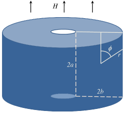
Figure 1: The physical setup proposed for the measurement of $\sigma_{xy}$.

$$H = \hbar v_{F}\left[\sigma_{1}\left(\frac{1}{i}\frac{\partial}{\partial x}-\frac{a}{\ell^{2}_{B}}\tan\phi\right)+\sigma_{2}\frac{1}{i}\frac{\partial}{\partial a\tan\phi}\right]+h_{z}\sigma_{3},\;\;\;\;\;-\phi_{0}<\phi<\phi_{0}$$ (2)

$$= \hbar v_{F}\left[\sigma_{1}\left(\frac{1}{i}\frac{\partial}{\partial x}-\frac{b}{\ell^{2}_{B}}\right)-\sigma_{2}\frac{1}{i}\frac{\partial}{\partial b\cot\phi}\right]-h_{z}\sigma_{1},\;\;\;\;\;\phi_{0}<\phi<\pi-\phi_{0}$$

$$= \hbar v_{F}\left[\sigma_{1}\left(\frac{1}{i}\frac{\partial}{\partial x}+\frac{a}{\ell^{2}_{B}}\tan\phi\right)+\sigma_{2}\frac{1}{i}\frac{\partial}{\partial a\tan\phi}\right]+h_{z}\sigma_{3}+V_{g},\;\;\;\;\;\pi-\phi_{0}<\phi<\pi+\phi_{0}$$

$$= \hbar v_{F}\left[\sigma_{1}\left(\frac{1}{i}\frac{\partial}{\partial x}+\frac{b}{\ell^{2}_{B}}\right)-\sigma_{2}\frac{1}{i}\frac{\partial}{\partial b\cot\phi}\right]+h_{z}\sigma_{1},\;\;\;\;\;\pi+\phi_{0}<\phi<2\pi-\phi_{0}.$$

where periodic boundary conditions for $x$, which is allowed to get arbitrarily large, are assumed. Obviously, the wavefunctions separate and correspond to planewaves with wavector $k$ in the $x$-coordinate. This will serve as the analog of the guiding center coordinate. The term proportional to $h_{z}$ represents the Zeeman coupling. A mean-field description of any possible quantum Hall ferromagnetism would have a different value of $h_{z}$ in the first and the third region than in the second and fourth. As usual, the magnetic length is $\ell_{B}=\sqrt{\hbar c/eB}$.

We can now find the eigenfunctions at a fixed energy $E$ and a fixed $k$ for each segment. This is done in detail in the Appendix. For the 1^st and 3^rd segment the Dirac eigenspinors can be written in a closed form in terms of the parabolic cylinder functions, $D_{\nu}(z)$, with indices $\nu$ of the upper and the lower components differing by $1$. For the 2^nd and 4^th segment, the eigenspinors are plane-waves. In what follows, we use dimensionless lengths and energy scales defined as

$$\alpha = \frac{a}{\ell_{B}},\;\beta=\frac{b}{\ell_{B}},\;\kappa=k\ell_{B}$$ (3)

$$\epsilon = \frac{E}{\hbar v_{F}/\ell_{B}},\;\eta_{z}=\frac{h_{z}}{\hbar v_{F}/\ell_{B}},\;\nu_{g}=\frac{V_{g}}{\hbar v_{F}/\ell_{B}}.$$ (4)

The matching of the wavefunction is discussed in detail below. While in general 4-parameter family of self-adjoined extensions is allowed, it is argued that for sharp edges, continuity of the wavefunctions should be imposed.

I.1 Matching conditions

In order to completely specify the behavior of the wavefunctions, the Hamiltonian (2) must be supplemented by boundary conditions at the points where the horizontal and the vertical surfaces meet. We will assume that the corners are sharp, meaning that the lengthscale associated with the corner curvature is much smaller than the magnetic length $\ell_{B}$.

If we require that the Hamiltonian is a self-adjoint operator we require that any two spinor wavefunctions $\psi_{1}$ and $\psi_{2}$ satisfy

$$\psi^{\dagger}_{1L}(\phi_{0})\sigma_{2}\psi_{2L}(\phi_{0}) = \psi^{\dagger}_{1R}(\phi_{0})\sigma_{2}\psi_{2R}(\phi_{0}),$$ (5)

where the subscripts $L$ and $R$ refer to the direction of approach of the boundary, i.e. left or rightStone and Goldbart (2009). The most general linear homogeneous boundary condition imposed on $\psi_{2}$ is

$$\psi_{2L} = M\psi_{2R},$$ (6)

where $M$ is a $2$ by $2$ matrix. In order to satisfy (5) we then must have

$$\psi^{\dagger}_{1L}(\phi_{0})\sigma_{2}M\psi_{2R}(\phi_{0}) = \psi^{\dagger}_{1R}(\phi_{0})\sigma_{2}\psi_{2R}(\phi_{0}).$$ (7)

This must hold for arbitrary $\psi_{2R}$ and therefore the boundary condition on $\psi_{1}$ is

$$\psi_{1R} = \sigma_{2}M^{\dagger}\sigma_{2}\psi_{1L}.$$ (8)

Since we require that the domains of $H$ and $H^{\dagger}$ coincide, the above must also be the boundary conditions on $\psi_{2}$. Therefore, $M$ must satisfy

$$M^{-1} = \sigma_{2}M^{\dagger}\sigma_{2}.$$ (9)

Taking the determinant of both sides gives

$$\frac{1}{\det M} = \det M^{*}\Rightarrow\det M=e^{i\chi}.$$ (10)

Using the above relations we finally find that

$$M = e^{\frac{i}{2}\chi}\left(\begin{array}[]{cc}W+Z&X-Y\\ X+Y&W-Z\end{array}\right),$$ (13)

$$1 = W^{2}-Z^{2}-X^{2}+Y^{2}.$$ (14)

That means that the self-adjoint constraint leaves us with $4$ independent real paraments which determine the boundary conditions at the corners. The von Neumann-Weyl deficiency indicesStone and Goldbart (2009) are therefore $(2,2)$

To determine these conditions we regularize the corners as small circles with the vertical and horizontal surface lines being tangential to the circle. Eventually, we are interested in taking the limit of the radius of the circle, $r_{0}$, to zero. Note that in the limit $r_{0}\ll\ell_{B}$ the vector potential does not depend on the position along the circle. As a result, the solution to the Dirac equation along the circle is a plane wave. The ratio of the two components of the Dirac spinor of the planewave solution is independent of the position, meaning that $X=Y=Z=0$. At finite energies the wave vector must be finite and therefore in the limit of $r_{0}\rightarrow 0$ the phase does not advance, i.e. $\chi=0$. This argument leads us to the requirement that for sharp corners, the Dirac spinors are continuous, or

$$M=1_{2}.$$ (15)

In addition, we are going to take the limit $b\gg\ell_{B}$ and focus on the solutions with the ”guiding center” $\kappa=k\ell_{B}$ either $\approx b/\ell=\beta$ or $\approx-\beta$. In the former case, $\kappa\approx\beta$, we can require that the wavefunction vanishes for $\tan\phi\rightarrow-\infty$ on the top surface and for $\tan\phi\rightarrow\infty$ on the bottom surface. Similarly, for $\kappa\approx-\beta$, we can require that the wavefunction vanishes for $\tan\phi\rightarrow\infty$ on the top surface and for $\tan\phi\rightarrow-\infty$ on the bottom surface.

II The energy spectrum

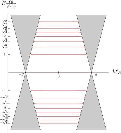
Figure 2: Energy spectrum for $h_{Z}=0$ and $a\rightarrow\infty$. In addition $\beta=b/\ell_{B}\gg 1$. The shaded cones represent the Dirac continuum physically located at the inner (left) and the outer (right) surfaces of the doubly connected sample. Each Landau level is doubly degenerate and at energy $\sqrt{2n}\hbar v_{F}/\ell_{B}$. To understand how the discrete Landau levels merge into the continuum, see Fig.4

The energy spectrum at each $k$ is determined from the matching conditions on the wavefunctions discussed above. Near each edge, these take the form of four linear equations in four unknowns (A.5) and (A.5), with energy and $k$ dependent coefficients. The technical details are presented in the Appendix. Here we present the analysis of the energy spectrum which results from these equations.

The non-trivial solution to the Eq.(A.5) exists provided that

$$\left[(\omega_{-}+i\theta_{-})\mathcal{B}_{+}-\epsilon\mathcal{A}_{+}\right]\left[(\omega_{-}-i\theta_{-})\mathcal{A}_{g+}-\epsilon\mathcal{B}_{g+}\right]e^{2i\theta_{-}\alpha}=$$

$$\left[(\omega_{-}-i\theta_{-})\mathcal{B}_{+}-\epsilon\mathcal{A}_{+}\right]\left[(\omega_{-}+i\theta_{-})\mathcal{A}_{g+}-\epsilon\mathcal{B}_{g+}\right]e^{-2i\theta_{-}\alpha}.$$

The functions used in the above equation are derived in the Appendix. The above equation determines the energy spectrum for $\kappa\approx\beta$, i.e. near the outer surface. If we are interested in the finite size effects, we have to keep $\alpha=a/\ell_{B}$ finite. This is useful to understand the degeneracy of each energy level caused by the tunneling across the vertical edge as well as mesoscopic transport effects discussed in the next section. On the other hand, in the thermodynamic limit $\alpha\rightarrow\infty$.

In order to solve Eq.(II) for $\epsilon=E/(v_{F}/\ell_{B})$ we need to consider two cases.

For $\theta^{2}_{-}>0$ the left hand side of Eq.(II) is the complex conjugate of the right hand side. Therefore, we are looking for roots of a purely imaginary function. Letting

$$\mathcal{S}=\left[(\omega_{-}+i\theta_{-})\mathcal{B}_{+}-\epsilon\mathcal{A}_{+}\right]\left[(\omega_{-}-i\theta_{-})\mathcal{A}_{g+}-\epsilon\mathcal{B}_{g+}\right],$$ (17)

we find that (II) requires

$$\tan\left(2\theta_{-}\alpha\right)=-\frac{\Im m\mathcal{S}}{\Re e\mathcal{S}}.$$ (18)

Note that the right hand side of the above equation does not depend on $\alpha$ while the left hand side has a single pole every time $2\theta_{-}\alpha=m\pi$ where $m=0,\pm 1,\pm 2\ldots$. For $\alpha\rightarrow\infty$ the spacing between the poles approaches zero and the left hand side changes from $-\infty$ to $\infty$ for $m\pi/(2\alpha)<\theta_{-}<(m+1)\pi/(2\alpha)$. Since the right hand side is a function of $\epsilon$ which changes on scales much larger than $1/\alpha$ as $\alpha\rightarrow\infty$, we have at least one positive and one negative eigenenergy solution for each interval $m\pi/(2\alpha)<\theta_{-}<(m+1)\pi/(2\alpha)$. This proves that for

$$\epsilon^{2}>(\kappa-\beta-\eta_{z})^{2}$$

the energy spectrum forms a continuum as $\alpha\rightarrow\infty$.

For $\theta^{2}_{-}<0$, the left hand side vanishes in the limit $\alpha\rightarrow\infty$ and the spectrum is determined by

$$\left[(\omega_{-}+|\theta_{-}|)\mathcal{B}_{+}-\epsilon\mathcal{A}_{+}\right]\left[(\omega_{-}-|\theta_{-}|)\mathcal{A}_{g+}-\epsilon\mathcal{B}_{g+}\right]=0.$$

For $\kappa-\beta\ll-1$, we can solve these equations within exponential accuracy by noting that for non-negative integer, the parabolic cylinder functions entering $\mathcal{A}_{+}$ and $\mathcal{B}_{+}$ satisfy

$$D_{\nu}(z) = 2^{-\nu/2}e^{-\frac{z^{2}}{4}}H_{\nu}\left(\frac{z}{\sqrt{2}}\right),\;\mbox{for}\;\nu=0,1,2,\ldots,$$

where $H_{n}(z)$ is Hermite polynomial. If the $\nu$ in $D_{\nu}(z)$ deviates from non-negative integer, the function diverges exponentially at large negative $z$. Therefore, as long as $\kappa-\beta\ll-1$, the equation

$$\left[(\omega_{-}+|\theta_{-}|)\mathcal{B}_{+}-\epsilon\mathcal{A}_{+}\right]=0$$

is solved for

$$\epsilon = \pm\sqrt{2n+\eta^{2}_{z}},\;\;\;n=1,2,3,\ldots,$$

$$\epsilon = -\eta_{z}.$$ (21)

Similarly, as long as $\kappa-\beta\ll-1$ the solutions to

$$\left[(\omega_{-}-|\theta_{-}|)\mathcal{A}_{g+}-\epsilon\mathcal{B}_{g+}\right]=0$$

are

$$\epsilon = \nu_{g}\pm\sqrt{2n+\eta^{2}_{z}},\;\;\;n=1,2,3,\ldots,$$

$$\epsilon = \nu_{g}+\eta_{z}.$$ (22)

For $\kappa\approx\beta$ the equations can be easily solved numerically and the dispersion of the Landau levels in the vicinity of the Dirac continuum can be determined. The solution for $\eta_{z}=\nu_{g}=0$ is shown in Fig.2 for both edges. In this case all Landau levels are doubly degenerate and the $\sigma_{xy}$ sequence is $\frac{e^{2}}{h}\times(\mbox{odd integer})$. Also, note the downward dispersion of the Landau levels as they approach the continuum. For $\eta_{z}=0.3$, $\nu_{g}=0$ the energy spectrum is shown in Fig. 3 for outer the edge. The lowest Landau level is now split linearly in $h_{z}$ giving rise to the possibility that if the Fermi energy lies in this gap $\sigma_{xy}=0$. The higher Landau levels are doubly degenerate, but split as they approach the edge continuum. Therefore for $\nu_{g}=0$, the allowed values for $\sigma_{xy}=ne^{2}/h$, are $n=0,\pm 1,\pm 3,\pm 5\ldots$. Finally, for $\nu_{g}\neq 0$ all possible Landau level (double) degeneracies are lifted, and as a result $n=0,\pm 1,\pm 2,\pm 3\ldots$.

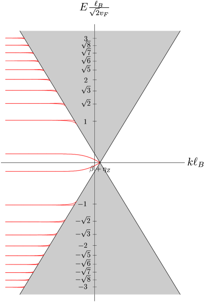
Figure 3: Energy spectrum for $h_{Z}\neq 0$ ($\eta_{z}=0.3$) and $a\rightarrow\infty$ near the outer surface. In addition $\beta=b/\ell_{B}\gg 1$. The shaded cones represent the Dirac continuum physically located at the outer surface. The degeneracy of the Landau levels is split as $\kappa=k\ell_{B}$ approaches the continuum. The double degeneracy of the zeroth Landau level is lifted, with a gap that varies linearly in $h_{Z}$. The double degeneracy of the higher Landau levels is split near the continuum, but in the thermodynamic limit remains intact for $\kappa\ll k\ell_{B}$ with the energies $\pm(\hbar v_{F}/\ell)\sqrt{2n+\eta^{2}_{z}}$, $n=0,1,2,\ldots$. The spectrum near the inner surface can be obtained simply by taking $\kappa\rightarrow-\kappa$, i.e. by mirror reflecting the above picture around $k\ell_{B}=0$.

Similarly, the non-trivial solution to the Eq.(A.5) exists provided that

$$\left[(\omega_{+}+i\theta_{+})\mathcal{B}_{-}-\epsilon\mathcal{A}_{-}\right]\left[(\omega_{+}-i\theta_{+})\mathcal{A}_{g-}-\epsilon\mathcal{B}_{g-}\right]e^{-2i\theta_{+}\alpha}=$$

$$\left[(\omega_{+}-i\theta_{+})\mathcal{B}_{-}-\epsilon\mathcal{A}_{-}\right]\left[(\omega_{+}+i\theta_{+})\mathcal{A}_{g-}-\epsilon\mathcal{B}_{g-}\right]e^{2i\theta_{+}\alpha}$$

The above equation determines the energy spectrum for $\kappa\approx-\beta$, i.e. near the inner surface. The analysis of this equation proceeds in the same way as for Eq.(II). The continuum appears for

$$\epsilon^{2}>(\kappa+\beta+\eta_{z})^{2}.$$

Furthermore, the equations for $\epsilon^{2}<(\kappa+\beta+\eta_{z})^{2}$ can be shown to be the same as (II) under the transformation $\kappa\rightarrow-\kappa$. The spectrum near the inner surface can therefore be determined simply by mirror reflecting the spectrum near outer surface about $\kappa=0$.

III Discussion of Hall bar vs. ”Corbino” geometry

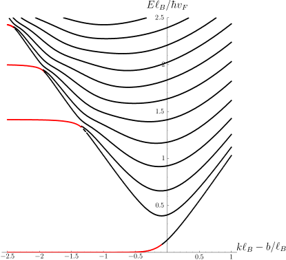
Figure 4: The positive energy spectrum for $h_{Z}=0$ and $\alpha=a/\ell_{B}=5$ near the outer surface. In addition $\beta=b/\ell_{B}\gg 1$. Note the presence of the discrete non-chiral modes, which merge into continuum for $\alpha\rightarrow\infty$. The spacing between the levels at $k\ell_{B}=b/\ell_{B}$ scales as $\sim 1/a$ while the spacing between the (Dirac) Landau levels for $k\ell_{B}\ll b/\ell_{B}$ scales as $\sim 1/\ell_{B}$. Therefore, in order to observe quantized Hall conductivity in the Hall bar geometry the condition $a\ll\ell_{B}$ should be satisfied.

$\begin{array}[]{cc}\includegraphics[width=108.405pt]{fig5a.eps}\\ \includegraphics[width=208.13574pt]{fig5b.epsi}\end{array}$

Figure 5: (Top panel) A schematic for a Hall bar setup for the 3D topological insulator. The applied magnetic field is perpendicular to the top surface. The applied magnetic field is perpendicular to the top surface; six contacts are also marked. (Bottom panel) The corresponding edge/surface state structure. There are $M$ chiral modes coming from the top and the bottom surface Hall droplet. In the absence of the bottom gate $M$ can be any odd integer (including zero if Zeeman field is included). In addition, there are $N$ non-chiral modes coming from the surfaces parallel to the external field.

Currently, the experimental geometry used to measure the Hall conductivity in the quantum Hall regime of 3D topological insulators is the Hall bar geometry sketched in Fig.5. No plateau quantization of $\sigma_{xy}$ has been observed. While part of the reason for this is finite 3D bulk conductivity, we wish to argue here that even if the system was insulating in the bulk the presence of the non-chiral surface modes will spoil the quantization of $\sigma_{xy}$. One way to avoid such contamination would be to reduce the sample height $\ll\ell_{B}$. The second way, would be to use ”Corbino” geometry shown in Fig.1, to ramp up the flux through the hollow region and to measure the charge transferred between the inner and the out surfaces.

For the Hall bar geometry in the ballistic limit, the Hall conductance, as well as the longitudinal conductance, are easily obtained within the Landauer-Buttiker formalism. Assuming that the contacts $2$, $3$, $5$ and $6$ float to the average chemical potential of the modes which enter them, for $M$-chiral modes and $N$-non-chiral modes with perfect transmission the Hall conductance, measured between contacts $2$ and $6$, is

$$G_{Hall} = \frac{e^{2}}{h}\left(M+N+\frac{N^{2}}{M}\right).$$ (24)

The longitudinal conductance measured between $2$ and $3$ is

$$G = \frac{e^{2}}{h}\left(2N+M+\frac{M^{2}}{N}+\frac{M^{2}}{N+M}\right).$$ (25)

For finite $N$, the Hall conductance here is generally not quantized. In the thermodynamic limit, $N\gg M$ and the Hall resistance is small ($\sim\frac{h}{e^{2}}M/N^{2}$). These results were also obtained in Ref.Zhang et al. (2011).

The physical reason for the non-quantization for large sample height is quite clear. The presence of the large number of non-chiral surface states tends to make the local potential on each of the surfaces close to $(\mu_{L}+\mu_{R})/2$, as opposed to $\mu_{L}$ on one, and $\mu_{R}$ on the other, as is the case in the absence of non-chiral modes. In the presence of disorder, in the form of scalar potential in the Dirac equation, but in the absence of electron-electron interactions, the states have been argued to remain delocalized Bardarson et al. (2007); Nomura et al. (2008) and the conductivity diverges as temperature $T\rightarrow 0$. Therefore in this limit there will be no voltage drop along the surfaces, all of which will appear near the contacts. The local potential near the two surfaces will still tend to $(\mu_{L}+\mu_{R})/2$ and no quantization of $G_{Hall}$ will occur. Including electron-electron interactions and scalar disorder, it has been argued in Ref.Ostrovsky et al. (2010) that the states remain delocalized, but that at $T=0$ the conductivity flows to a finite value. Therefore, the potential will drop along the surfaces, the modes will equilibrate but no quantization will occur. The two terminal conductance will also not be quantizedLee (2009). The way to achieve quantization in the Hall bar geometry is therefore to eliminate the side surface modes altogether, which can be achieved through finite size effects by reducing the height of the sample below $\ell_{B}$.

A four terminal setup shown in Fig.6a of Ref.Zhang et al. (2011) has been argued to lead to quantized Hall conductance $Me^{2}/h$ even in the presence of disorder. However, this result was obtained assuming that the number of non-chiral channels is exactly $N$ for each of the four segments of the four terminal setup. Unlike the number of chiral channels $M$, for a thick sample the number of non-chiral channels can vary from segment to segment. In the four terminal setup, we should therefore consider $N_{1}$ channels between $\mu_{L}$ and $\mu_{2}$, $N_{2}$ between $\mu_{2}$ and $\mu_{R}$, $N_{3}$ between $\mu_{R}$ and $\mu_{4}$ and $N_{4}$ between $\mu_{4}$ and $\mu_{L}$. In the ideal case of perfect transmission, we find $I_{4}-I_{2}=\frac{e^{2}}{h}\left(2M+N_{1}-N_{2}+N_{3}-N_{4}\right)(\mu_{L}-\mu_{2})$. Therefore, unless $N_{1}-N_{2}=N_{4}-N_{3}$, the Hall conductance defined this way is not properly given by the number of chiral channels. As mentioned in the introduction, for typical Fermi momentumBrüne et al. (2011); Xiong et al. (2011) $k_{F}\sim 0.2-0.5nm^{-1}$, this would require a few $nm$ precision in the height of the sample. It seems that, in the least, such sensitivity to surface roughness would have to be eliminated in practice.

In the Corbino geometry, the increase of the flux will transfer the charge from the inner to the outer surface, which can then measured. In the thermodynamic limit, this quantization is robust to the presence non-chiral states. Such measurement of $\sigma_{xy}$ has been performed in 2DEGs (Ref.Dolgopolov et al. (1992)) where both integer and fractional quantizations have been detected, and should be feasible in the 3D topological insulators in the quantum Hall regime.

Appendix A Derivation of the Hamiltonian, eigenstates and the matching conditions

In this appendix we present the detailed steps which lead to the Eq.(2) as well as to the matching conditions which lead to the equation for the energy spectrum. We use the parametrization shown in Fig.1.

A.1 Top horizontal surface ($-\phi_{0}<\phi<\phi_{0}$)

For the top horizontal surface, $r(\phi)=a/\cos\phi$ and $-\phi_{0}<\phi<\phi_{0}$ where $\tan\phi_{0}=b/a$. For $\phi$ in this range the metric for the surface is

$$ds^{2} = dx_{1}^{2}+dx_{2}^{2}=dx^{2}+\left[r^{2}(\phi)+\left(\frac{dr(\phi)}{d\phi}\right)^{2}\right]d\phi^{2}$$ (26)

$$= dx^{2}+\left(da\tan\phi\right)^{2}.$$

In the Landau gauge of choice here, the two components of the vector potential are

$$A_{1} = Ba\tan\phi,\;\;A_{2}=0.$$ (27)

The physical spin is related to the Dirac Pauli matrices byLee (2009)

$$\vec{s}=\hat{n}\times\vec{\sigma}$$ (28)

where $\hat{n}$ is the normal to the surface. Using $\hat{n}=\hat{z}$ and $s_{1}s_{2}=is_{3}$, we obtain

$$s_{1} = -\sigma_{2},\;\;s_{2}=\sigma_{1},\;\;s_{3}=\sigma_{3}.$$ (29)

Thus, for $-\phi_{0}<\phi<\phi_{0}$ the Hamiltonian is

$$H = \hbar v_{F}\left[\sigma_{1}\left(\frac{1}{i}\frac{\partial}{\partial x}-\frac{a}{\ell^{2}_{B}}\tan\phi\right)+\sigma_{2}\frac{1}{i}\frac{\partial}{\partial a\tan\phi}\right]+h_{z}\sigma_{3}.$$

$\ell_{B}=\sqrt{\frac{\hbar c}{eB}}$. This is clearly separable, and the eigenfunctions are planewaves in the $x-$ direction. Its wavevector is set to be $k$. Letting $\rho=\sqrt{2}\left(\frac{a}{\ell_{B}}\tan\phi-k\ell_{B}\right)$ leads to

$$\left(\begin{array}[]{cc}h_{z}-E&-\sqrt{2}\frac{\hbar v_{F}}{\ell_{B}}\left(\frac{\partial}{\partial\rho}+\frac{1}{2}\rho\right)\\ \sqrt{2}\frac{\hbar v_{F}}{\ell_{B}}\left(\frac{\partial}{\partial\rho}-\frac{1}{2}\rho\right)&-h_{z}-E\end{array}\right)\left(\begin{array}[]{c}u_{k}(\phi)\\ v_{k}(\phi)\end{array}\right)=0.$$ (35)

The generic solution to these two coupled first order differential equations is

$$\left(\begin{array}[]{c}u_{k}(\phi)\\ v_{k}(\phi)\end{array}\right)=c_{1,L}\left(\begin{array}[]{c}\alpha_{1}D_{\nu}(\rho)\\ \beta_{1}D_{\nu+1}(\rho)\end{array}\right)+c_{1,R}\left(\begin{array}[]{c}\alpha_{2}D_{\nu}(-\rho)\\ \beta_{2}D_{\nu+1}(-\rho)\end{array}\right),$$ (42)

where $D_{\nu}(\rho)$ is the parabolic cylinder function Merzbacher (1998)

$$D_{\nu}(\rho) = 2^{\nu/2}e^{-\rho^{2}/4}\left[\frac{\Gamma[\frac{1}{2}]}{\Gamma[(1-\nu)/2]}{{}_{1}}F_{1}\left(-\frac{\nu}{2};\frac{1}{2};\frac{\rho^{2}}{2}\right)\right.$$ (43)

$$\left.\frac{\rho}{\sqrt{2}}\frac{\Gamma[-\frac{1}{2}]}{\Gamma[-\nu/2]}{{}_{1}}F_{1}\left(\frac{1-\nu}{2};\frac{3}{2};\frac{\rho^{2}}{2}\right)\right]$$

and ${{}_{1}}F_{1}$ is the confluent hypergeometric function

$${{}_{1}}F_{1}\left(a;b;\rho\right)=1+\frac{a}{c}\frac{\rho}{1!}+\frac{a(a+1)}{c(c+1)}\frac{\rho^{2}}{2!}+\ldots.$$ (44)

Unless $\nu$ is a non-negative integer, the two solutions in the Eq.(42) are linearly independent and $D_{\nu}(\rho)$ diverges as $\rho\rightarrow-\infty$. These functions satisfy the relations

$$\left(\frac{\partial}{\partial\rho}+\frac{1}{2}\rho\right)D_{\nu}(\rho) = \nu D_{\nu-1}(\rho),$$ (45)

$$\left(\frac{\partial}{\partial\rho}-\frac{1}{2}\rho\right)D_{\nu}(\rho) = -D_{\nu+1}(\rho).$$ (46)

Since we are interested in taking the limit $b\gg\ell_{B}$, the solution near the outer surface must satisfy vanishing boundary condition as it moves closer to the 2D ”bulk”. This means that near the outer surface $c_{1,L}=0$ and

$$\left(\begin{array}[]{c}u_{k}(\phi)\\ v_{k}(\phi)\end{array}\right)=c_{1,R}\left(\begin{array}[]{c}(\epsilon+\eta_{z})D_{\frac{1}{2}(\epsilon^{2}-\eta_{z}^{2})-1}\left(\sqrt{2}\left(\kappa-\alpha\tan\phi\right)\right)\\ \sqrt{2}D_{\frac{1}{2}(\epsilon^{2}-\eta_{z}^{2})}\left(\sqrt{2}\left(\kappa-\alpha\tan\phi\right)\right)\end{array}\right),$$ (51)

where the dimensionless lengths and energy scales are $\alpha=\frac{a}{\ell_{B}}$, $\beta=\frac{b}{\ell_{B}}$, $\kappa=k\ell_{B}$, $\epsilon=\frac{E}{\hbar v_{F}/\ell_{B}}$, $\eta_{z}=\frac{h_{z}}{\hbar v_{F}/\ell_{B}}$ and $\nu_{g}=\frac{V_{g}}{\hbar v_{F}/\ell_{B}}$.

Similarly, near the inner surface $c_{1,R}=0$ and the solution has the form

$$\left(\begin{array}[]{c}u_{k}(\phi)\\ v_{k}(\phi)\end{array}\right)=$$ (57)

$$c_{1,L}\left(\begin{array}[]{c}-(\epsilon+\eta_{z})D_{\frac{1}{2}(\epsilon^{2}-\eta^{2}_{z})-1}\left(\sqrt{2}(\alpha\tan\phi-\kappa)\right)\\ \sqrt{2}D_{\frac{1}{2}(\epsilon^{2}-\eta^{2}_{z})}\left(\sqrt{2}(\alpha\tan\phi-\kappa)\right)\end{array}\right).$$

A.2 Outer vertical surface ($\phi_{0}<\phi<\pi-\phi_{0}$)

$r(\phi)=b/\sin\phi$

$$ds^{2} = dx_{1}^{2}+dx_{2}^{2}=dx^{2}+\left(db\cot\phi\right)^{2}$$ (58)

$$\Rightarrow x_{1} = x,\;\;\;x_{2}=a+b-b\cot\phi.$$ (59)

$$A_{1} = Bb,\;\;A_{2}=0.$$ (60)

The physical spin operators (up to $\hbar/2$) are

$$s_{1} = \sigma_{3},\;\;s_{2}=\sigma_{2},\;\;s_{3}=-\sigma_{1}.$$ (61)

For $\phi_{0}<\phi<\pi-\phi_{0}$ the Hamiltonian is

$$H = \hbar v_{F}\left[\sigma_{1}\left(\frac{1}{i}\frac{\partial}{\partial x}-\frac{eB}{\hbar c}b\right)-\sigma_{2}\frac{1}{i}\frac{\partial}{\partial b\cot\phi}\right]-h_{z}\sigma_{1}.$$

and the eigenfunctions are

$$\left(\begin{array}[]{c}u_{k}(\phi)\\ v_{k}(\phi)\end{array}\right) = c_{2,1}e^{i\sqrt{\epsilon^{2}-(\kappa-\beta-\eta_{z})^{2}}\beta\cot\phi}\left(\begin{array}[]{c}\alpha_{+}\\ \epsilon\end{array}\right)$$ (67)

$$+ c_{2,2}e^{-i\sqrt{\epsilon^{2}-(\kappa-\beta-\eta_{z})^{2}}\beta\cot\phi}\left(\begin{array}[]{c}\alpha_{-}\\ \epsilon\end{array}\right),$$ (70)

where

$$\alpha_{\pm}=\kappa-\beta-\eta_{z}\pm i\sqrt{\epsilon^{2}-(\kappa-\beta-\eta_{z})^{2}}.$$ (71)

A.3 Bottom horizontal surface ($\pi-\phi_{0}<\phi<\pi+\phi_{0}$)

$r(\phi)=-a/\cos\phi$

$$ds^{2} = dx_{1}^{2}+dx_{2}^{2}=dx^{2}+\left(da\tan\phi\right)^{2}$$ (72)

$$\Rightarrow x_{1} = x,\;\;\;x_{2}=2(a+b)+a\tan\phi.$$ (73)

$$A_{1} = -Ba\tan\phi,\;\;A_{2}=0.$$ (74)

$$s_{1} = \sigma_{2},\;\;s_{2}=-\sigma_{1},\;\;s_{3}=\sigma_{3}.$$ (75)

For $\pi-\phi_{0}<\phi<\pi+\phi_{0}$ the Hamiltonian is

$$H = \hbar v_{F}\left[\sigma_{1}\left(\frac{1}{i}\frac{\partial}{\partial x}+\frac{a}{\ell^{2}_{B}}\tan\phi\right)+\sigma_{2}\frac{1}{i}\frac{\partial}{\partial a\tan\phi}\right]$$ (76)

$$+ h_{z}\sigma_{3}+V_{g}.$$

where we included a different electrical potential on the bottom surface $V_{g}$.

Near the outer vertical surface the solution on the bottom horizontal surface is

$$\left(\begin{array}[]{c}u_{k}(\phi)\\ v_{k}(\phi)\end{array}\right)=$$ (79)

$$c_{3,R}\left(\begin{array}[]{c}\sqrt{2}D_{\frac{1}{2}((\epsilon-\nu_{g})^{2}-\eta_{z}^{2})}\left(\sqrt{2}\left(\kappa+\alpha\tan\phi\right)\right)\\ (\epsilon-\eta_{z}-\nu_{g})D_{\frac{1}{2}((\epsilon-\nu_{g})^{2}-\eta_{z}^{2})-1}\left(\sqrt{2}\left(\kappa+\alpha\tan\phi\right)\right)\end{array}\right),$$ (82)

where $\nu_{g}=V_{g}/(\hbar v_{F}/\ell_{B})$.

Near the inner vertical surface the solution on the bottom horizontal surface is

$$\left(\begin{array}[]{c}u_{k}(\phi)\\ v_{k}(\phi)\end{array}\right)=$$ (85)

$$c_{3,L}\left(\begin{array}[]{c}\sqrt{2}D_{\frac{1}{2}\left((\epsilon-\nu_{g})^{2}-\eta^{2}_{z}\right)}\left(-\sqrt{2}(\kappa+\alpha\tan\phi)\right)\\ (\nu_{g}-\epsilon+\eta_{z})D_{\frac{1}{2}\left((\epsilon-\nu_{g})^{2}-\eta^{2}_{z}\right)-1}\left(-\sqrt{2}(\kappa+\alpha\tan\phi)\right)\end{array}\right).$$ (88)

A.4 Inner vertical surface ($\pi+\phi_{0}<\phi<2\pi-\phi_{0}$)

$r(\phi)=-b/\sin\phi$

$$ds^{2} = dx_{1}^{2}+dx_{2}^{2}=dx^{2}+\left(db\cot\phi\right)^{2}$$ (89)

$$\Rightarrow x_{1} = x,\;\;\;x_{2}=3(a+b)-b\cot\phi.$$ (90)

$$A_{1} = -Bb,\;\;A_{2}=0.$$ (91)

$$s_{1} = -\sigma_{3},\;\;s_{2}=\sigma_{2},\;\;s_{3}=\sigma_{1}.$$ (92)

For $\pi+\phi_{0}<\phi<2\pi-\phi_{0}$ the Hamiltonian is

$$H = \hbar v_{F}\left[\sigma_{1}\left(\frac{1}{i}\frac{\partial}{\partial x}+\frac{b}{\ell^{2}_{B}}\right)-\sigma_{2}\frac{1}{i}\frac{\partial}{\partial b\cot\phi}\right]+h_{z}\sigma_{1}.$$

The eigenfunctions are

$$\left(\begin{array}[]{c}u_{k}(\phi)\\ v_{k}(\phi)\end{array}\right) = c_{4,1}e^{i\sqrt{\epsilon^{2}-(\kappa+\beta+\eta_{z})^{2}}\beta\cot\phi}\left(\begin{array}[]{c}\alpha_{+}\\ \epsilon\end{array}\right)$$ (98)

$$+ c_{4,2}e^{-i\sqrt{\epsilon^{2}-(\kappa+\beta+\eta_{z})^{2}}\beta\cot\phi}\left(\begin{array}[]{c}\alpha_{-}\\ \epsilon\end{array}\right),$$ (101)

where

$$\alpha_{\pm}=\kappa+\beta+\eta_{z}\pm i\sqrt{\epsilon^{2}-(\kappa+\beta+\eta_{z})^{2}}.$$ (102)

A.5 Matching conditions

As discussed in the main text, we require the continuity of the wavefunctions near the outer surface where $\kappa\approx\beta$. Therefore, we must have

$$\left(\begin{array}[]{c}u_{k}(\phi^{(-)}_{0})\\ v_{k}(\phi^{(-)}_{0})\end{array}\right) = \left(\begin{array}[]{c}u_{k}(\phi^{(+)}_{0})\\ v_{k}(\phi^{(+)}_{0})\end{array}\right)$$ (107)

$$\left(\begin{array}[]{c}u_{k}(\pi-\phi^{(+)}_{0})\\ v_{k}(\pi-\phi^{(+)}_{0})\end{array}\right) = \left(\begin{array}[]{c}u_{k}(\pi-\phi^{(-)}_{0})\\ v_{k}(\pi-\phi^{(-)}_{0})\end{array}\right),$$ (112)

where $\phi^{(\pm)_{0}}=\phi_{0}\pm 0^{+}$.

Using the wavefunctions determined in the Appendix, the above set of four linear equations in four unknowns translates into

$$\mathcal{A}_{+}c_{1,R} = e^{i\theta_{-}\alpha}(\omega_{-}+i\theta_{-})c_{2,1}+e^{-i\theta_{-}\alpha}(\omega_{-}-i\theta_{-})c_{2,2}$$

$$\mathcal{B}_{+}c_{1,R} = e^{i\theta_{-}\alpha}\epsilon c_{2,1}+e^{-i\theta_{-}\alpha}\epsilon c_{2,2}$$

$$\mathcal{B}_{g+}c_{3,R} = e^{-i\theta_{-}\alpha}(\omega_{-}+i\theta_{-})c_{2,1}+e^{i\theta_{-}\alpha}(\omega_{-}-i\theta_{-})c_{2,2}$$

$$\mathcal{A}_{g+}c_{3,R} = e^{i\theta_{-}\alpha}\epsilon c_{2,1}+e^{-i\theta_{-}\alpha}\epsilon c_{2,2}$$ (113)

where

$$\mathcal{A}_{\pm} = \pm(\epsilon+\eta_{z})D_{\frac{1}{2}(\epsilon^{2}-\eta^{2}_{z})-1}\left(\sqrt{2}(-\beta\pm\kappa)\right)$$ (114)

$$\mathcal{B}_{\pm} = \sqrt{2}D_{\frac{1}{2}(\epsilon^{2}-\eta^{2}_{z})}\left(\sqrt{2}(-\beta\pm\kappa)\right)$$ (115)

$$\mathcal{A}_{g\pm} = \pm(\epsilon-\nu_{g}-\eta_{z})D_{\frac{1}{2}((\epsilon-\nu_{g})^{2}-\eta^{2}_{z})-1}\left(\sqrt{2}(-\beta\pm\kappa)\right)$$

$$\mathcal{B}_{g\pm} = \sqrt{2}D_{\frac{1}{2}((\epsilon-\nu_{g})^{2}-\eta^{2}_{z})}\left(\sqrt{2}(-\beta\pm\kappa)\right)$$ (117)

$$\omega_{\pm} = \kappa\pm\beta\pm\eta_{z}$$ (118)

$$\theta_{\pm} = \sqrt{\epsilon^{2}-\omega^{2}_{\pm}}.$$ (119)

Near the inner surface, where $\kappa\approx-\beta$, we must have

$$\left(\begin{array}[]{c}u_{k}(\pi+\phi^{(-)}_{0})\\ v_{k}(\pi+\phi^{(-)}_{0})\end{array}\right) = \left(\begin{array}[]{c}u_{k}(\pi+\phi^{(+)}_{0})\\ v_{k}(\pi+\phi^{(+)}_{0})\end{array}\right)$$ (124)

$$\left(\begin{array}[]{c}u_{k}(2\pi-\phi^{(+)}_{0})\\ v_{k}(2\pi-\phi^{(+)}_{0})\end{array}\right) = \left(\begin{array}[]{c}u_{k}(-\phi^{(-)}_{0})\\ v_{k}(-\phi^{(-)}_{0})\end{array}\right),$$ (129)

This translates to

$$\mathcal{B}_{g-}c_{3,L} = e^{i\theta_{+}\alpha}(\omega_{+}+i\theta_{+})c_{4,1}+e^{-i\theta_{+}\alpha}(\omega_{+}-i\theta_{+})c_{4,2}$$

$$\mathcal{A}_{g-}c_{3,L} = e^{i\theta_{+}\alpha}\epsilon c_{4,1}+e^{-i\theta_{+}\alpha}\epsilon c_{4,2}$$

$$\mathcal{A}_{-}c_{1,L} = e^{-i\theta_{+}\alpha}(\omega_{+}+i\theta_{+})c_{4,1}+e^{i\theta_{+}\alpha}(\omega_{+}-i\theta_{+})c_{4,2}$$

$$\mathcal{B}_{-}c_{1,L} = e^{-i\theta_{+}\alpha}\epsilon c_{4,1}+e^{i\theta_{+}\alpha}\epsilon c_{4,2}$$

References

• Lee (2009) D.-H. Lee, Phys. Rev. Lett. 103, 196804 (2009).
• Dolgopolov et al. (1992) V. T. Dolgopolov, A. A. Shashkin, N. B. Zhitenev, S. I. Dorozhkin, and K. von Klitzing, Phys. Rev. B 46, 12560 (1992).
• Fu et al. (2007) L. Fu, C. L. Kane, and E. J. Mele, Phys. Rev. Lett. 98, 106803 (2007).
• Fu and Kane (2007) L. Fu and C. L. Kane, Phys. Rev. B 76, 045302 (2007).
• Hsieh et al. (2008) D. Hsieh, D. Qian, L. Wray, Y. Xia, Y. S. Hor, R. J. Cava, and M. Z. Hasan, Nature 452, 970 (2008).
• Hsieh et al. (2009) D. Hsieh, Y. Xia, L. Wray, D. Qian, A. Pal, J. H. Dil, J. Osterwalder, F. Meier, G. Bihlmayer, C. L. Kane, et al., Science 323, 919 (2009).
• Xia et al. (2009) Y. Xia, D. Qian, D. Hsieh, L. Wray, A. Pal, H. Lin, A. Bansil, D. Grauer, Y. S. Hor, R. J. Cava, et al., Nature Physics 5, 398 (2009).
• Chen et al. (2009) Y. L. Chen, J. G. Analytis, J.-H. Chu, Z. K. Liu, S.-K. Mo, X. L. Qi, H. J. Zhang, D. H. Lu, X. Dai, Z. Fang, et al., Science 325, 178 (2009).
• Qi and Zhang (2010) X. L. Qi and S. Zhang, Physics Today 63, 33 (2010).
• Moore (2010) J. Moore, Nature 464, 194 (2010).
• Hasan and Kane (2010) M. Z. Hasan and C. L. Kane, Rev. Mod. Phys. 82, 3045 (2010).
• Chu et al. (2011) R.-L. Chu, J. Shi, and S.-Q. Shen, Phys. Rev. B 84, 085312 (2011).
• Yang and Han (2011) Z. Yang and J. H. Han, Phys. Rev. B 83, 045415 (2011).
• Zhang et al. (2011) Y.-Y. Zhang, X.-R. Wang, and X. C. Xie, ArXiv e-prints (2011), eprint 1103.3761v2.
• Nomura et al. (2008) K. Nomura, S. Ryu, M. Koshino, C. Mudry, and A. Furusaki, Phys. Rev. Lett. 100, 246806 (2008).
• Taskin and Ando (2009) A. A. Taskin and Y. Ando, Phys. Rev. B 80, 085303 (2009).
• Checkelsky et al. (2009) J. G. Checkelsky, Y. S. Hor, M.-H. Liu, D.-X. Qu, R. J. Cava, and N. P. Ong, Phys. Rev. Lett. 103, 246601 (2009).
• Analytis et al. (2010) J. G. Analytis, R. D. McDonald, S. C. Riggs, J. H. Chu, G. S. Boebinger, and I. R. Fisher, Nature Physics 6, 960 (2010).
• Xiong et al. (2011) J. Xiong, A. C. Petersen, D. Qu, R. J. Cava, and N. P. Ong, ArXiv e-prints (2011), eprint 1101.1315.
• Qu et al. (2011) D.-X. Qu, Y. S. Hor, R. J. Cava, and N. P. Ong, ArXiv e-prints (2011), eprint 1108.4483.
• Brüne et al. (2011) C. Brüne, C. X. Liu, E. G. Novik, E. M. Hankiewicz, H. Buhmann, Y. L. Chen, X. L. Qi, Z. X. Shen, S. C. Zhang, and L. W. Molenkamp, Phys. Rev. Lett. 106, 126803 (2011).
• Pnueli (1994) A. Pnueli, Journal of Physics A: Mathematical and General 27, 1345 (1994).
• Stone and Goldbart (2009) M. Stone and P. M. Goldbart, Mathematics for Physics: A Guided Tour for Graduate Students (Cambridge University Press, 2009), 1st ed.
• Bardarson et al. (2007) J. H. Bardarson, J. Tworzydło, P. W. Brouwer, and C. W. J. Beenakker, Phys. Rev. Lett. 99, 106801 (2007).
• Ostrovsky et al. (2010) P. M. Ostrovsky, I. V. Gornyi, and A. D. Mirlin, Phys. Rev. Lett. 105, 036803 (2010).
• Sitte et al. (2011) M. Sitte, A. Rosch, E. Altman, and L. Fritz, ArXiv e-prints (2011), eprint 1110.1363v1.
• Merzbacher (1998) E. Merzbacher, Quantum Mechanics (John Wiley & Sons, New York, NY, USA, 1998), 3rd ed.