Magnetic field decay in neutron stars: from Soft Gamma Repeaters to “weak field magnetars”

Abstract

The recent discovery of the “weak field, old magnetar”, the soft gamma repeater SGR 0418+5729 , whose dipole magnetic field, $B_{\rm dip}$, is less than $7.5\times 10^{12}\;$G , has raised perplexing questions: How can the neutron star produce SGR-like bursts with such a low magnetic field? What powers the observed X-ray emission when neither the rotational energy nor the magnetic dipole energy are sufficient? These observations, that suggest either a much larger energy reservoir or a much younger true age (or both), have renewed the interest in the evolutionary sequence of magnetars. We examine, here, a phenomenological model for the magnetic field decay: $\dot{B}_{\rm dip}\propto B_{\rm dip}^{1+\alpha}$ and compare its predictions with the observed period, $P$, the period derivative, $\dot{P}$, and the X-ray luminosity, $L_{X}$, of magnetar candidates. We find a strong evidence for a dipole field decay on a timescale of $\sim 10^{3}\;$yr for the strongest ($B_{\rm dip}\sim 10^{15}\;$G) field objects, with a decay index within the range $1\leq\alpha<2$ and more likely within $1.5\lesssim\alpha\lesssim 1.8$. The decaying field implies a younger age than what is implied by $P/2\dot{P}$. Surprisingly, even with the younger age, the energy released in the dipole field decay is insufficient to power the X-ray emission, suggesting the existence of a stronger internal field, $B_{\rm int}$. Examining several models for the internal magnetic field decay we find that it must have a very large ($\gtrsim 10^{16}\;$G) initial value. Our findings suggest two clear distinct evolutionary tracks – the SGR/AXP branch and the transient branch, with a possible third branch involving high-field radio pulsars that age into low luminosity X-ray dim isolated neutron stars.

1 Introduction

Soft Gamma Repeaters (SGRs) and Anomalous X-ray Pulsars (AXPs) are two classes of pulsating X-ray sources thought to be highly magnetized Neutron Stars (NSs) whose high-energy emission is powered by the dissipation of their magnetic field. Hence they are deemed magnetars. They have large rotation periods ($5\;{\rm s}\lesssim P\lesssim 12\;$s) with relatively large time derivatives ($\dot{P}\sim 10^{-12}-10^{-10}\;{\rm s\;s^{-1}}$), implying (through magnetic dipole breaking) large surface dipole field strengths ($B_{\rm dip}\gtrsim 3\times 10^{14}\;$G or energy $E_{\rm B_{\rm dip}}\gtrsim 2\times 10^{46}\;$erg) and relatively young spindown ages ($\tau_{\rm c}\sim 10^{3}-10^{5}\;$yr). Thus, the decay of their dipole fields on the timescale of their spindown ages appears to be capable of accounting for their large persistent X-ray luminosities, of $L_{\rm X}\sim 10^{35}$ erg s^-1 (Thompson & Duncan, 1995). On the other hand, rotational energy losses are 1-2 orders of magnitude too low to account for their measured $L_{\rm X}$, and the absence of binary companions strongly argues against accretion as a power source.

Both SGRs and AXPs can emit sporadic, sub-second ($\sim 0.1\;$s) bursts of hard X-rays to soft $\gamma$-rays, which release $\sim 10^{38}-10^{41}\;$erg at typically super-Eddington luminosities. Evolving stresses from a decaying magnetic field $>10^{14}\;$G can in principle stress the rigid lattice of the NS crust beyond its yielding point, leading to sudden release of stored magnetic energy, which is believed to trigger these bursts (Thompson & Duncan, 1996; Perna & Pons, 2011).

AXPs tend to be less burst-active, and have somewhat weaker dipole fields and larger spindown ages compared to SGRs. This led to the suggestion that SGRs evolve into AXPs as they age and their magnetic field decays (Kouveliotou et al., 1998). The effect of the decay of the dipole magnetic field on the spin evolution of magnetars was previously considered (Colpi et al., 2000), but its ultimate implications for their expected X-ray emission have not yet been fully explored.

In addition to classical SGRs and AXPs, the magnetar family includes also transient sources. First discovered in 2003 (XTE J1810-197; Ibrahim et al. 2004), the group of transients is now the largest among magnetar candidates and is rapidly growing, thanks to the improved detection capabalities of the Fermi Gamma-ray Burst Monitor (GBM). The distinctive property of transients is that they are discovered only thanks to outbursts, when they emit typical magnetar-like bursts accompanied by a very large increase ($\sim$ two orders of magnitude) of their persistent emission. Their timing parameters can only be measured in outburst and they match well those of persistent SGRs/AXPs. The implied rotational energy losses are much lower than the outburst-enhanced persistent emission. However, when the much weaker quiescent emission of transients could eventually be measured, it was found to be below the level of rotational energy losses.

Typical magnetar-like bursts and outburst was also detected from the 0.3 s, allegedly rotation-powered X-ray pulsar PSR J1846-0258, with a dipole field of $4.8\times 10^{13}$ G (Gavriil et al., 2008; Kumar & Safi-Harb, 2008), and the radio pulsar PSR 1622-4950, with a spin period of 4.3 s and a dipole field of $3\times 10^{14}$ G, displayed a flaring radio emission (Levin et al., 2010), with properties very similar to those of two transient radio magnetars (Camilo et al., 2006, 2007). On the other hand, there are radio pulsars with dipole fields comparable to the weaker field magnetars, and larger than PSR J1846-0258, but showing no sign of peculiar behaviour. Thus, a strong dipole field does not seem a sufficient condition for powering magnetar-like emission (Kaspi, 2010).

The greatest surprise, however, came from the recent discovery of SGR 0418+5729 by the Fermi Gamma-ray Burst Monitor . This source, previously undetected in X-rays, was discovered on 5 June, 2009, through the emission of two distinct, sub-second magnetar-like bursts of low luminosity ($\lesssim 10^{38}$ erg s^-1) and total energy $\sim 2{\rm~{}and}~{}4\times 10^{37}$ erg, (van der Horst et al., 2010). Following the bursts it became detectable as a bright, pulsating X-ray source with a period of $\sim$9.1 s and a luminosity of $L_{\rm X}\approx 10^{34}$ erg s^-1 that decayed by 2 orders of magnitude during the following 6 months (Esposito et al., 2010). However, only an upper limit could be put on its period derivative, $\dot{P}<6\times 10^{-15}\;{\rm s\;s^{-1}}$, translating to an upper limit of $B_{\rm dip}<7.5\times 10^{12}\;$G on its dipole field strength and a spindown age $\tau_{\rm c}>24\;$Myr (Rea et al., 2010). This demonstrates that magnetar-like activity can be present in NSs with rather standard dipole magnetic fields. This finding represents a breakthrough in our understanding of magnetars, as it was unexpected that bursts could be produced in such a low-field object, if they are associated with sudden crustal fractures.

Moreover, it is clear that the dipole field of SGR 0418+5729 cannot power its X-ray emission if it decays on the timescale of its spindown age (of $\tau_{\rm c}>24\;$Myr). The latter would require a much stronger field, of $\gtrsim 5\times 10^{14}\;$G, in order to power the weakest level of X-ray emission at which this source was found, 1.5 yr after the outburst (Rea et al., 2010). That is, either its total magnetic energy is $>$5000 times larger than that the dipole (Turolla et al., 2011), or its dipole field decay time is $>$5000 times smaller than its spindown age (or some combination of the two).

Bearing on the above arguments, we address, in this work the power source of magnetar candidates and their spin evolution as their dipole fields decay. The latter are jointly compared with the observed properties of the full sample of magnetar candidates, thus enabling us to draw robust conclusions. In § 2 we describe the main properties of the different classes of objects of interest and our observed sample. In § 3 we provide a simple analytic formalism for the spin evolution of NSs whose dipole field decays as $\dot{B}_{\rm dip}=-B_{\rm dip}/\tau_{\rm d}\propto B_{\rm dip}^{1+\alpha}$, and discuss its general properties. A summary of the mechanisms for magnetic field decay in NSs is provided in § 4. In § 5 we show that there is indeed a strong evidence for effective decay of the dipole fields of these sources, which is $\sim 10^{3}\;$yr timescale for the strongest fields of SGRs and AXPs, and provide quantitative constraints on the most likely decay mechanisms (we show that $1\lesssim\alpha<2$ is required). These constraints are made tighter ($1.5\lesssim\alpha\lesssim 1.8$) in § 6, where we show that decay of the dipole component alone is insufficient to power the X-ray emission and that a stronger power source is required, presumably a stronger internal magnetic field. We examine two models for internal magnetic field decay in § 7. Comparing with observations we derive basic constraints on the initial values and decay properties of such a component. Our conclusions are summarized in § 8. Finally, in § 9 we build on our conclusions to outline a self-consistent evolutionary scenario for magnetar candidates and speculate about their relation to other classes of objects.

2 Source classes and the observational sample

In order to verify the role of field decay in NSs with strong magnetic fields we consider here the X-ray and timing properties of magnetar candidates. These are usually identified by their measured values of $P$ and $\dot{P}$ (hence the inferred dipole field, $B_{\rm dip}$, and spin-down age, $\tau_{c}$), detection of peculiar burst/outburst activity and persistent X-ray luminosities that exceed rotational energy losses. Sources are divided into two main groups, largely for historical reasons. SGRs are typically identified by the emission of trains of sporadic, sub-second bursts of X-to-$\gamma$-ray radiation with super-Eddington luminosities ($\sim 10^{39}-10^{42}$ erg s^-1). More rarely they show much more powerful events, the Giant Flares (GFs). These are typically initiated by a spike of $\gamma$-ray emission lasting half a second and releasing $\sim 10^{44}-10^{46}$ erg at luminosities $\sim 10^{44}-10^{47}$ erg s^-1 (assuming isotropic emission), which are followed by minute-long, yet super-Eddington, tails of radiation ($\sim 10^{41}-10^{42}$ erg s^-1), markedly pulsed at the NS spin (Mazets et al., 1979; Cline et al., 1998; Hurley et al., 1999; Terasawa et al., 2005; Palmer et al., 2005).

The highly super-Eddington luminosities of bursts and GFs definitely rules out accretion as a viable power source. Indeed, it first hinted to the key role of superstrong magnetic fields which reduce the electron scattering cross-section much below the Thomson value. In particular, $B\gtrsim 3\times 10^{14}$ G were required to explain luminosities up to $10^{42}$ erg s^-1 (Paczynski, 1992). The several minute-long pulsating tails are very similar in all three GFs detected so far. They suggest that a remarkably standard amount of energy, $\sim{\rm a~{}few}\times 10^{44}$ erg, remains trapped in a small-size, closed field line region in the magnetosphere ($\sim$ a few stellar radii), likely in the form of a pair-photon plasma, and slowly radiated away (the “trapped fireball” model of Thompson & Duncan 1995). A magnetospheric field $\gtrsim{\rm a~{}few}\times 10^{14}$ G would naturally account for this.

Anomalous X-ray Pulsars were typically identified through the peculiar properties of their persistent emission (Mereghetti & Stella, 1995). However, the distinction between these two classes has come into question since SGR-like bursting activity has been detected in many APXs (Gavriil et al., 2002; Woods & Thompson, 2006; Mereghetti, 2008). To date, AXP have never displayed a GF and are, in general, characterized by less frequent, and somewhat less energetic, burst activity.

There are persistent and transient sources both in the SGR and the AXP classes. The emission from the persistent sources is known to be pulsed at the NS spin period and to be characterized by a blackbody (BB) component, with $kT\sim 0.4\,$–$\,0.7\;$keV, plus a power-law (PL) tail extending up to $\sim 10\;$keV (Mereghetti (2008) and references therein). In recent years, a new power-law component extending up to $\sim$ 150 keV was discovered with the INTEGRAL satellite (Kuiper et al. (2006); for recent reviews Woods & Thompson (2006), Mereghetti 2008). This component has a very flat $\nu F_{\nu}$ spectrum and is thus clearly distinct from the lower energy PL. A seizable fraction of the bolometric emission from SGRs/AXPs is emitted in the 10 - 150 keV energy range, and it is likely comparable to that at lower energies, below $10\;$keV (Mereghetti, 2008). The persistent emission of these sources gets temporarily enhanced at bursts (SGRs/AXPs) and Flares (SGRs only), but such variations are usually moderate – normally at most by a factor of a few.

Transient sources, on the other hand, are characterized by a much weaker persistent X-ray emission, which in some cases still remains undetected. When detected, it is generally found to be at a lower level than rotational energy losses ($L_{\rm X}<|\dot{E}_{\rm rot}|$). Transient sources are distinctively characterized by X-ray outbursts during which, in addition to the emission of sub-second long bursts (similar to the bursts of persistent sources), their persistent X-ray emission is subject to very large enhancements, by $\sim 2\,$–$\,3$ orders of magnitude, making them temporarily as bright as the persistent sources. In fact, most of these objects have been discovered thanks to such events. In outburst, their luminosities largely exceed rotational energy losses ($L_{\rm X,outburst}\gg|\dot{E}_{\rm rot}|$), and gradually return to the much lower quiescent level over timescales of $\sim$ a few years (cfr. Rea & Esposito (2011) for a recent review).Data for persistent SGRs/AXPs and transient sources were collected from the McGill catalog.

In addition to these “classical” magnetar candidates, we consider the properties of X-ray Dim Isolated NSs (XDINs; Kaplan (2008); Mereghetti (2011), Kaplan & van Kerkwijk 2011). These are a class of currently seven, $\sim 10^{6}$ yr old X-ray sources, which are considered as neat examples of isolated, cooling NSs. They have stable and nearly purely thermal persistent emission (but see, e.g. Turolla 2009), typically described as a single BB with $kT\sim 0.05\,$–$\,0.1\;$keV. Their spin periods are in the same range as SGRs/AXPs and their inferred dipole fields are all $>10^{13}$ G. As such, a possible link with magnetar candidates has long been suspected. Data collected for all sources are summarized in Table 1.

	$P$	$\dot{P}$	$L_{X}$	$kT$	$\tau_{c}$	$|\dot{E}_{\rm rot}|$	$B_{\rm dip}$	$a\equiv$	$k\equiv$	$f_{A}\equiv$
Name	(s)	($10^{-11}\,{\rm s/s}$)	($10^{35}\,{\rm erg/s}$)	(keV)	(kyr)	($10^{33}\,{\rm erg/s}$)	($10^{14}\,$G)	$L_{X}\tau_{c}/E_{\rm dip}$	$L_{X}/|\dot{E}_{\rm rot}|$	$\frac{L_{X}}{4\pi R^{2}\sigma T^{4}}$
SGR 1086$-$20	7.6022(7)	75(4)	1.6	$0.6^{+0.2}_{-0.1}$	0.16	67	24	0.00083	2.4	0.096
SGR 0526$-$66	8.0544(2)	3.8(1)	1.4		3.4	2.9	5.6	0.28	49	0.32
SGR 1900$+$14	5.19987(7)	9.2(4)	0.83–1.3	0.47(2)	0.90	26	7.0	0.037	4.1	$\sim$0.17
SGR 1627$-$41	2.594578(9)	1.9(4)	$\sim$0.025		2.2	43	2.2	0.020	0.058
SGR 0418$+$5729	9.07838827(4)	$<$0.0006	0.00062	0.67(11)	$>$24000	$<$0.00032	$<$0.075	$>$5050	$>$196	0.000024
SGR 1833$-$0832	7.565408(4)	0.439(43)			27	0.40	1.8
1E 1547$-$5408	2.06983302(4)	2.318(5)	$\sim$0.0058	0.43(4)	1.4	100	2.2	0.0032	0.0056	0.0013
XTE J1810$-$197	5.5403537(2)	0.777(3)	$\sim$0.0019	0.14–0.30	11	1.8	2.1	0.0092	0.11	0.0063
1E 1048$-$5937	6.45207658(54)	$\sim$2.70	0.054	0.623(6)	3.8	3.9	4.2	0.022	1.4	0.0028
1E 2259$+$586	6.9789484460(39)	0.048430(8)	0.18	0.411(4)	230	0.056	0.59	225	320	0.049
CXOU J010043.1$-$72134	8.020392(6)	1.88(8)	$\sim$0.78	0.38(2)	6.8	1.4	3.9	0.65	54	0.29
4U 0142$+$61	8.68832973(8)	0.1960(2)	$>$0.53	0.395(5)	70	0.12	1.3	$>$40	$>$449	$>$0.17
CXO J164710.2$-$455216	10.6107(1)	0.083(2)	$\sim$0.0044	0.49(1)	200	0.027	0.95	1.7	16.3	0.0006
1RXS J170849.0$-$400910	10.9990355(6)	1.945(2)	$\sim$1.9	0.456(9)	9.0	0.57	4.7	1.47	329	0.34
1E 1841$-$045	11.7750542(1)	4.1551(14)	$\sim$2.2	0.44(2)	4.5	0.99	7.1	0.37	219	0.45
PSR J1622$-$4950	4.3261(1)	1.7(1)	$\sim$0.0063	$\sim$0.4	4.0	8.5	2.8	0.0064	0.076	0.0019
CXOU J171405.7$-$381031	3.82535(5)	6.40(14)	$\sim$2.2	0.38(8)	0.95	45	5.0	0.16	4.9	0.82
RXJ 1856	7.05	0.003	0.00017	0.063	3700	0.0034	0.15	55	5.0	0.084
RXJ 0720	8.39	0.00698(2)	0.00337	0.090(5)	1900	0.0047	0.25	202	72	0.40
RXJ 1605	6.88		0.00011$d_{0.1}^{2}$	0.096						0.010
RXJ 0806	11.37	0.006	0.00033	0.096	3000	0.0016	0.26	27	20	0.030
RXJ 1308	10.31	0.011	0.000051$d_{0.1}^{2}$	0.102	1500	0.0040	0.34	1.2$d_{0.1}^{2}$	1.3$d_{0.1}^{2}$	0.0036$d_{0.1}^{2}$
RXJ 2143	9.44	0.004	$\geq$0.00069	0.100	3700	0.0019	0.20	$\geq$126	$\geq$37	$\geq$0.053
RXJ 0420	3.45	0.00028	0.00032	0.044	2000	0.027	0.1	115.2	1.18	0.66

Table 1: Summary of the salient timing and X-ray spectral properties of SGRs, AXPs and XDINs. Data are collected from references cited in the text.

Although timing data are homogeneuos and can be easily compared for all classes above, significantly different values of $\dot{P}$ have been measured at different epochs in SGR 1806-20 and 1900+14, leading to different values of the inferred dipole fields. We show in all plots the maximum and minimum value of the inferred $B_{\rm dip}$, for either object, joined by a dotted line. In the following discussion we consider, however, the lowest value as a more likely indication of the dipole field (cfr. Thompson et al. (2002); Woods & Thompson (2006) for discussion of magnetic torque changes).

Data on the X-ray emission from different classes, on the other hand, must be compared with caution. Important spectral differences exist and, in some cases, marked temporal variability makes the sample much less homogeneous. We adopt the X-ray luminosity in the $(2\,$–$\,10$) keV range, as reported in the McGill catalog, as a measure of the thermal emission from persistent sources, which we call $L_{\rm X}$. Given their typical BB temperatures, bolometric corrections are expected to be $\sim\,2\,$–$\,4$ and will be ignored. Note that the contribution from the PL component in this energy range is not negligible either, which at least partially balances for the neglect of bolometric corrections. Also note that GFs might provide a non-negligible contribution to $L_{\rm tot}$ in SGRs, and that the hard tails up to $\gtrsim 150$ keV also contribute significantly to the latter.

The quiescent emission of transients is less clearly understood. In most of them it appears dominated by a BB component with temperature ($\sim 0.4$ keV) and an emitting area much smaller than the NS surface. The resulting luminosities are generally $\lesssim 10^{33}$ erg s^-1, and the bolometric corrections to their ($2-10$) keV emission are thus similar to those of persistent sources.

In XTE J1810, on the other hand, the BB component which dominates the quiescent emission has a much lower temperature, $kT\simeq 0.18$ keV and an emitting area consistent with the NS surface (Bernardini et al., 2009). This implies a total luminosity $\lesssim 10^{33}$ erg s^-1, but a relatively large bolometric correction to the $(2-10)$ keV flux.

As we see later the ”weak field magnetar” SGR 0418+5729, with its extreme parameters, plays a very important role in constraining various models. Particularly important is its total X-ray luminosity, $L_{\rm tot}$. The current observed value of $\simeq 6\times 10^{31}$ erg s^-1 in the $(0.5-10)$ keV range (Rea et al., 2010) might well be a post flare remnant emission larger than its real quiescent level, which is unknown. It is interesting to use the energy budget of its recent outburst to estimate a minimal average power needed. The decaying X-ray flux following the outburst was monitored from June 2009 to September 2010 (Esposito et al., 2010). Results of this monitoring allow to estimate a total fluence in the $0.5\,$–$\,10\;$keV energy range corresponding to $\Delta E\simeq 3\times 10^{40}\;$erg, for a distance of 2 kpc to this source. Even if the outburst recurrence time was $T_{\rm rec}\sim 100\;$yr, this would still correspond to an average luminosity of $\langle L_{\rm outb}\rangle\sim 10^{31}\;{\rm erg\;s^{-1}}$ due only to such outbursts, not much below the current upper limit.

Does such a recurrence time match what we know about outbursts from transient sources? If $T_{\rm age}$ is the age of SGR 0418+5729 and $T_{\rm birth}$ is the average time between the birth of magnetars in our Galaxy, one expects a rate of outbursts of $R_{\rm outb}=10\,T_{\rm age,Myr}(T_{\rm birth,kyr}~{}T_{\rm rec,100})^{-1}\;{\rm yr^{-1}}$ in the Galaxy. The age of SGR 0418+5729 could be as small as $\approx 0.1\;$Myr (based on the upper limit on its quiescent X-ray luminosity, as we discuss in next sections) but, on the other hand, their actual birth rate is likely to be a few times larger than our adopted lower limit of 1 per kyr (Gaensler et al., 1999). The ratio $T_{\rm age}/T_{\rm birth}$ is thus not expected to vary much, in any case. Comparing with observations, we note that outbursts from 4 different sources were detected, in one year of operation, by the Fermi satellite. Two of these sources were previously unknown and could not have been detected if they had been further than a few kpc, and are thus detectable only from a small fraction of our Galaxy (van der Horst et al., 2010). This matches reasonably well our estimate of $R_{\rm outb}$, thus supporting our estimate of $\langle L_{\rm outb}\rangle$.

We finally note that uncertain distance determinations can affect the inferred luminosities. For most objects, different estimates agree to within factors $<1.5$. Although non-negligible, this typically translates to uncertainties of a factor $\lesssim 2$ on $L_{X}$. The AXP 1E 1048-5937 represents, however, a notable exception. Durant & van Kerkwijk (2006) find a distance of $9.0\pm 1.7\;$kpc for this source, based on a detailed study of reddening of red giant stars in the field of this AXP. This is significantly larger than the $2.7\pm 0.1\;$kpc reported in the McGill catalogue (Gaensler et al., 2005). The persistent X-ray luminosity of 1E 1048-5937 would accordingly increase by a factor $\sim 11$, reaching the value $L_{X}\sim 6\times 10^{34}\;{\rm erg\;s^{-1}}$ instead of $\sim 5\times 10^{33}\;{\rm erg\;s^{-1}}$ as reported in the McGill catalog. We consider both values for this source.

3 Magnetic dipole braking and field decay

The energy loss rate of a magnetic dipole rotating in vacuum is:

$$L_{\rm vac}=\frac{2}{3}\frac{\mu^{2}\Omega^{4}}{c^{3}}\sin^{2}\theta_{\rm B}\ ,$$ (1)

where $\theta_{\rm B}$ is the angle between the dipole and rotation axes.

$$\mu=B_{\rm eq}R^{3}=\frac{1}{2}B_{\rm pol}R^{3}\ ,$$ (2)

is the magnetic moment, where $R$ is the stellar radius while $B_{\rm eq}$ and $B_{\rm pol}$ are the surface magnetic field strengths at the dipole equator and pole, respectively. More realistically, however, a magnetized rotating neutron star is surrounded by plasma rather than vacuum. Three dimensional (3D) force-free numerical simulation (Spitkovsky, 2006) have shown that this slightly increases the energy loss rate to:

$$L_{\rm pls}=\frac{\mu^{2}\Omega^{4}}{c^{3}}(1+\sin^{2}\theta_{\rm B})\ .$$ (3)

The evolution of the spin period $P$ is governed by $L_{\rm pls}=-\dot{E}_{\rm rot}=-I\Omega\dot{\Omega}=I(2\pi)^{2}\dot{P}/P^{3}$, or:

$$\frac{d}{dt}\left(P^{2}\right)=2P\dot{P}=\frac{8\pi^{2}\mu^{2}}{Ic^{3}}(1+\sin^{2}\theta_{\rm B})=\frac{8\pi^{2}B_{\rm eq}^{2}R^{6}}{Ic^{3}}(1+\sin^{2}\theta_{\rm B})\equiv f\,\frac{8\pi^{2}B_{\rm eq}^{2}R^{6}}{Ic^{3}}\ .$$ (4)

Values of $B_{\rm eq}$ for isolated, spinning down NSs are usually estimated through this formula, using the measured values of the spin period, $P$, and its first derivative, $\dot{P}$. Generally the formula for an orthogonal rotator in vacuum is used (Eq. [1], with $\theta_{\rm B}=90^{\circ}$). That expression is formally recovered from the more realistic one given in Eq. (3) by taking $f=2/3$. In what follows we will maintain the explicit dependence on $f$ for all quantities but always specialize to the case $f=2/3$ when making numerical estimates. Defining a characteristic spindown age, $\tau_{\rm c}=P/(2\dot{P})$, Eq. (4) can be rearranged to read:

$$B_{\rm eq}=\left(\frac{Ic^{3}}{f8\pi^{2}R^{6}}\right)^{1/2}\frac{P}{\tau^{1/2}_{\rm c}}\ .$$ (5)

We shall now allow the dipole magnetic field to evolve in time in the above equations and use its value at the equator as our reference field strength from here on, $B_{\rm eq}(t)\equiv B_{\rm dip}(t)$. For simplicity, however, the angle $\theta_{\rm B}$ and thus also the factor $f=1+\sin^{2}\theta_{\rm B}$ will be taken to be constant in time. The exact solution for the spin period becomes:

$$P^{2}(t)=P^{2}(t_{0})+f\,\frac{8\pi^{2}R^{6}}{Ic^{3}}\int_{t_{0}}^{t}B_{\rm dip}^{2}(t^{\prime})dt^{\prime}\ .$$ (6)

The spindown depends in a critical way on the time-dependence of magnetic dipole energy, $E_{\rm dip}\propto B_{\rm dip}^{2}$, since this determines the behaviour of the integral on the right-hand side.

Following the notations and parameterization introduced by Colpi et al. (2000), we write:

$$\frac{dB_{\rm dip}}{dt}=-AB_{\rm dip}^{1+\alpha}=-\frac{B_{\rm dip}}{\tau_{\rm d}(B_{\rm dip})}\ ,$$ (7)

where we define the field decay timescale $\tau_{\rm d}(B_{\rm dip})\equiv(AB_{\rm dip}^{\alpha})^{-1}$. The solution of Eq. (7) is:

$$B_{\rm dip}(t)=B_{\rm dip,i}\left\{\matrix{(1+\alpha\,t/\tau_{\rm d,i})^{-1/\alpha}\quad&(\alpha\neq 0)&\ ,\cr\exp(-t/\tau_{\rm d,i})\quad&(\alpha=0)&\ ,}\right.$$ (8)

where $B_{\rm dip,i}=B_{\rm dip}(t=0)$ is the initial dipole field strength, and $\tau_{\rm d,i}=\tau_{\rm d}(B_{\rm dip,i})=1/AB_{\rm dip,i}^{\alpha}$ is the initial field decay time. Note that $\alpha=0$, which corresponds to an exponential field decay on the timescale $\tau_{\rm d,exp}=1/A$, is the only value of $\alpha$ for which $\tau_{\rm d}$ remains constant. We do not consider $\alpha<0$ (for which the field vanishes within a finite time, $t=-\tau_{\rm d,i}/\alpha$). Substituting Eq. (8) into Eq. (6) gives:

$$P^{2}(t)=P_{i}^{2}+f\frac{8\pi^{2}R^{6}_{*}}{Ic^{3}}B^{2}_{\rm dip,i}\tau_{\rm d,i}\left\{\matrix{\frac{1}{2-\alpha}\left[1-(1+\alpha t/\tau_{\rm d,i})^{(\alpha-2)/\alpha}\right]\quad&(\alpha\neq 0,\,2)\ ,\cr\frac{1}{2}\left[1-\exp(-2t/\tau_{\rm d,i})\right]\quad&(\alpha=0)\ ,\cr\frac{1}{2}\ln(1+2t/\tau_{\rm d,i})\quad&(\alpha=2)\ ,}\right.$$ (9)

where $P_{i}=P(t=0)$ is the initial spin period, at the birth of the NS. For $0\leq\alpha<2$ the spindown essentially freezes out at late times (or at very late times for $\alpha$ close to 2) and the rotation period $P$ appraoches a constant value,

$$P_{\infty}^{2}=P_{i}^{2}+f\frac{8\pi^{2}R^{6}}{Ic^{3}}B^{2}_{\rm dip,i}\frac{\tau_{\rm d,i}}{(2-\alpha)}\ .$$ (10)

The field decay thus proceeds at a nearly constant spin at such late times. Usually $P_{\infty}\gg P_{i}$, and in this case:

$$P_{\infty}\simeq\sqrt{\frac{f\,8\pi^{2}R^{6}}{Ic^{3}(2-\alpha)}}\,B_{\rm dip,i}\tau^{1/2}_{\rm d,i}\approx\frac{7.65\;{\rm s}}{\sqrt{2-\alpha}}f^{1/2}R^{3}_{6}I^{-1/2}_{45}B_{\rm i,15}\left(\frac{\tau_{\rm d,i}}{10^{3}~{}{\rm yrs}}\right)^{1/2}\propto B_{\rm dip,i}^{\frac{2-\alpha}{2}}\ ,$$ (11)

where hereafter we use the notation $Q_{n}=10^{n}\times Q$ in c.g.s units.

It is convenient to rewrite Eq. (7) in terms of the spindown time, $\tau_{c}=P/(2\dot{P})$, using the relation $dB_{\rm dip}/d\tau_{c}=\dot{B}_{\rm dip}{\rm d}\tau_{c}/{\rm dt}$:

$$\frac{dB_{\rm dip}}{d\tau_{c}}=-\frac{B_{\rm dip}}{\tau_{d}}\frac{1}{1+2(\tau_{c}/\tau_{d})}\ .$$ (12)

For the initial conditions $\tau_{c}=\tau_{\rm c,i}$, $B_{\rm dip}=B_{\rm dip,i}$ and $\tau_{\rm d}=\tau_{\rm d,i}$ at $t=0$, the solution to this equation is:

$$\tau_{c}(B_{\rm dip})=\left\{\matrix{\frac{\tau_{\rm d,i}}{2-\alpha}\left\{\left[1+(2-\alpha)\frac{\tau_{\rm c,i}}{\tau_{\rm d,i}}\right]\left(\frac{B_{\rm dip,i}}{B_{\rm dip}}\right)^{2}-\left(\frac{B_{\rm dip,i}}{B_{\rm dip}}\right)^{\alpha}\right\}\quad&(\alpha\neq 2)\ ,\cr\cr\left(\frac{B_{\rm dip,i}}{B_{\rm dip}}\right)^{2}\left[\tau_{\rm c,i}+\tau_{\rm d,i}\ln\left(\frac{B_{\rm dip,i}}{B_{\rm dip}}\right)\right]\quad&(\alpha=2)\ .\cr}\right.$$ (13)

Substitution of Eq. (8) into this solution yields:

$$\tau_{c}(t)=\left\{\matrix{\frac{\tau_{\rm d,i}}{2-\alpha}\left\{\left[1+(2-\alpha)\frac{\tau_{\rm c,i}}{\tau_{\rm d,i}}\right]\left(1+\frac{\alpha t}{\tau_{\rm d,i}}\right)^{2/\alpha}-\left(1+\frac{\alpha t}{\tau_{\rm d,i}}\right)\right\}\quad&(\alpha\neq 0,\,2)\ ,\cr\cr\frac{\tau_{\rm d,i}}{2}\left\{\left[1+\frac{2\tau_{\rm c,i}}{\tau_{\rm d,i}}\right]\exp\left(\frac{2t}{\tau_{\rm d,i}}\right)-1\right\}\quad&(\alpha=0)\ ,\cr\cr\left(1+\frac{2t}{\tau_{\rm d,i}}\right)\left[\tau_{\rm c,i}+\frac{\tau_{\rm d,i}}{2}\ln\left(1+\frac{2t}{\tau_{\rm d,i}}\right)\right]\quad&(\alpha=2)\ .\cr}\right.$$ (14)

For the specific case of $\alpha=0$ the expression for $\tau_{c}(t)$ in Eq. (14) can be easily inverted to obtain:

$$t(\tau_{c})=\frac{\tau_{\rm d,i}}{2}\ln\left(\frac{1+\frac{2\tau_{c}}{\tau_{\rm d,i}}}{1+\frac{2\tau_{\rm c,i}}{\tau_{\rm d,i}}}\right)\ ,$$ (15)

but this is not possible for a general value of $\alpha$. Nevertheless, at early times we can write:

$$\tau_{c}(t\ll\tau_{\rm d,i}/\alpha)\approx\tau_{\rm c,i}+t\ .$$ (16)

Equations (5) and (10) imply that:

$$(2-\alpha)\frac{\tau_{\rm c,i}}{\tau_{\rm d,i}}=\left[\left(\frac{P_{\infty}}{P_{i}}\right)^{2}-1\right]^{-1}\approx\left(\frac{P_{i}}{P_{\infty}}\right)^{2}\ .$$ (17)

Since one expects $P_{i}\ll P_{\infty}$, then the term in Eqs. (13)–(15) involving the initial conditions (i.e. that with $\tau_{\rm c,i}$) can be neglected at $t\gg\tau_{\rm c,i}$, where $\tau_{c}(\tau_{\rm c,i}\ll t\ll\tau_{\rm d,i}/\alpha)\approx t$.

The limits of the expressions above at late times, $t\gg\tau_{\rm d,i}/\alpha$, are:

$$B_{\rm dip}(t\gg\tau_{\rm d,i}/\alpha)\approx B_{\rm dip,i}\left\{\matrix{(\alpha\,t/\tau_{\rm d,i})^{-1/\alpha}\quad&(\alpha>0)&\ ,\cr\exp(-t/\tau_{\rm d,i})\quad&(\alpha=0)&\ }\right.$$ (18)

and

$$P(t\gg\tau_{\rm d,i}/\alpha)\approx\left\{\matrix{P_{\infty}(\alpha)\left[1-\frac{1}{2}\exp(-2t/\tau_{\rm d,i})\right]\approx P_{\infty}(\alpha)\quad&(\alpha=0)\ ,\cr P_{\infty}(\alpha)\left[1-\frac{1}{2}(\alpha t/\tau_{\rm d,i})^{(\alpha-2)/\alpha}\right]\sim P_{\infty}(\alpha)\quad&(0<\alpha<2)\ ,\cr P_{\infty}(\alpha=0)\sqrt{\ln(2t/\tau_{\rm d,i})}\quad&(\alpha=2)\ ,\cr P_{\infty}(4-\alpha)\,(\alpha t/\tau_{\rm d,i})^{(\alpha-2)/2\alpha}\quad&(\alpha>2)\ .}\right.$$ (19)

For $\alpha>2$ the period grows at late times as $P\propto t^{(\alpha-1)/2\alpha}$. This reproduces the familiar $\dot{P}\propto P^{-1}$ evolution for spin-down at a constant magnetic field ($\alpha\to\infty$). For $0\leq\alpha<2$, $P$ approaches $P_{\infty}$ at late times. We note, however, that for $0<2-\alpha\ll 1$ the asymptotic spin period $P_{\infty}$ is approached extremely slowly, where $P(t)/P_{\infty}\approx g<1$ at $t\approx(\tau_{\rm d,i}/\alpha)(1-g)^{-\alpha/(2-\alpha)}\to(\tau_{\rm d,i}/2)(1-g)^{-2/(2-\alpha)}$, e.g. $P$ reaches half of its asymptotic value at $t\approx(\tau_{\rm d,i}/\alpha)2^{\alpha/(2-\alpha)}\to\tau_{\rm d,i}2^{2/(2-\alpha)}$. When $P_{\infty}$ is approached, then Eq. (5) (or equivalently, Eq. [13]) implies that:

$$B_{\rm dip}=\sqrt{\frac{Ic^{3}}{f\,8\pi^{2}R^{6}}}\,\frac{P_{\infty}}{\tau^{1/2}_{c}}=1.07\times 10^{15}f^{-1/2}I_{45}^{1/2}R_{6}^{-3}\left(\frac{P_{\infty}}{10~{}\rm s}\right)\left(\frac{\tau_{c}}{1\;{\rm kyr}}\right)^{-1/2}\;{\rm G}\ ,$$ (20)

Note that, although this expression is independent on $\alpha$, it holds only for $\alpha<2$. This simple scaling will indeed hold for any scenario in which the spin period freezes, provided the appropriate value of $P_{\infty}$ is used. In fact, it corresponds to the general relation 5, with the spin period kept constant to the asymptotic value.

From Eqs. (13) and (14) we obtain the late time behaviour of $\tau_{c}$, at $B_{\rm dip}\ll B_{\rm dip,i}$ or $t\gg\tau_{\rm d,i}$:

$$\tau_{c}\approx\left\{\matrix{\frac{\tau_{\rm d,i}}{2}\left(\frac{B_{\rm dip,i}}{B_{\rm dip}}\right)^{2}&\approx&\frac{\tau_{\rm d,i}}{2}\exp\left(\frac{2t}{\tau_{\rm d,i}}\right)\quad&(\alpha=0)\ ,\cr\cr\frac{\tau_{\rm d,i}}{2-\alpha}\left(\frac{B_{\rm dip,i}}{B_{\rm dip}}\right)^{2}&\approx&\frac{\tau_{\rm d,i}}{2-\alpha}\left(\frac{\alpha t}{\tau_{\rm d,i}}\right)^{2/\alpha}\quad&(0<\alpha<2)\ ,\cr\cr\tau_{\rm d,i}\left(\frac{B_{\rm dip,i}}{B_{\rm dip}}\right)^{2}\ln\left(\frac{B_{\rm dip,i}}{B_{\rm dip}}\right)&\approx&t\ln\left(\frac{2t}{\tau_{\rm d,i}}\right)\quad&(\alpha=2)\ ,\cr\cr\frac{\tau_{\rm d,i}}{\alpha-2}\left(\frac{B_{\rm dip,i}}{B_{\rm dip}}\right)^{\alpha}&\approx&\frac{\alpha}{\alpha-2}t\quad&(\alpha>2)\ ,}\right.$$ (21)

The are summarized in Fig. 1 summarizes the main results of this section. It shows the expected relation $B_{\rm dip}$ vs. $\tau_{c}$ and the evolution of the ratio $(t/\tau_{\rm c})$ with $\tau_{c}$, for 4 different values of $\alpha\leq 2$. All plots are obtained for the same initial value $B_{\rm dip,i}=10^{15}$ G and assume a normalization of the decay time, $\tau_{\rm d,i}=10^{3}{\rm yrs}/B^{\alpha}_{\rm i,15}$ yrs.

Figure 1: Different cases of field decay with asymptotic spin period. Left Panel: Dipole magnetic field, $B_{\rm dip}$, as a function of spindown age, $\tau_{\rm c}$, for 4 selected values of the decay index, $\alpha\leq 2$. All curves have the same initial $B_{\rm dip,i}=10^{15}\;$G. Smaller values of the asymptotic period $P_{\infty}$ correspond to lower asymptotic curves where $B_{\rm dip}\propto P_{\infty}/\sqrt{\tau_{\rm c}}$. Right Panel: The ratio $t/\tau_{\rm c}$ between real age and spindown age as a function of the spindown age, for the same models. The $y$-axis gives the correction factor that must be applied to the measured spindown age, $\tau_{\rm c}$, to derive the real age of an object. Lower values of $\alpha$ correspond to much younger objects, at a given $\tau_{\rm c}$, because they produce a faster decay of the field and, accordingly, of $\dot{P}$.

4 Summary of physical mechanisms causing field decay

General modes of fied decay in non-superfluid NS interiors were studied by Goldreich & Reisenegger 1992 (GR92 hereafter), who identified three avenues for field evolution: Ohmic decay, ambipolar diffusion and Hall drift. While the first two mechanisms are intrinsically dissipative, leading directly to a decrease in field energy, the third one is not. GR92 proved its potential relevance, however, for the transport and dissipation of magnetic energy within NS crusts (cfr. Jones 1988), by speeding up ohmic dissipation of the field.

The analysis by GR92 showed that ambipolar diffusion is conveniently split in two different components, according to their effect on the stable stratification of NS core matter. The solenoidal component does not perturb chemical equilibrium of particle species, thus its evolution is opposed only by particle collisions. The irrotational mode does perturb chemical equilibrium, so it also activates $\beta$-reactions in the NS core. At high temperatures ($T>7\times 10^{8}$ K) the two modes are degenerate, as $\beta$-reactions are very efficient and particle collisions represent the only effective force against which ambipolar diffusion works (GR92, TD96) The distinction between the two components becomes essential at lower temperature, as perturbations of the chemical equilibrium are not erased quickly, thus significantly slowing down the irrotational mode (GR92, TD96). Following GR92, the relevant timescales for the two modes of ambipolar diffusion can be written as:

$$\tau^{(\rm s)}_{\mbox{\tiny{ambi}}} \simeq 3\times 10^{3}\frac{L^{2}_{5}T^{2}_{8}}{B^{2}_{15}}~{}\mbox{~{}yr}$$

$$\tau^{(\rm ir)}_{\mbox{\tiny{ambi}}} \simeq \frac{5\times 10^{9}}{T^{6}_{8}B^{2}_{15}}~{}\mbox{~{}yr}+\tau^{(s)}_{\mbox{\tiny{ambi}}}~{}~{}.$$ (22)

Note the strikingly different dependence on temperature of the two modes, which turns out to be a key factor. Since field dissipation releases heat in the otherwise cooling core, a balance between field-decay heating and neutrino cooling (through modified URCA reactions) is expected to be reached. This determines an equilibrium relation between core temperature and strength of the core magnetic field. The two following relations, for either mode, are obtained (TD96; Dall’Osso et al. 2009, hereafter DSS09):

$$T^{(\rm s)}_{8,{\rm eq}} \simeq 2.7~{}B^{2/5}_{15}\left(\frac{\rho_{15}}{0.7}\right)^{-2/3}\ ,$$

$$T^{(\rm ir)}_{8,{\rm eq}} \simeq 2.4\left(\frac{B}{10^{2}~{}B_{\rm QED}}\right)^{2}\left(\frac{\rho_{15}}{0.7}\right)^{-1}\ ,$$ (23)

where $\rho_{15}$ is the density of matter normalized to $10^{15}$ g cm^-3. Using these relations we eventually obtain expressions for the relavant timescales as a function of $B$ alone:

$$\tau^{(s)}_{\rm ambi} \simeq \frac{1.5\times 10^{5}}{B^{6/5}_{15}}\left(\frac{\rho_{15}}{0.7}\right)^{-2/5}~{}\mbox{~{}yrs}~{}~{}~{}~{}~{}~{}(\alpha=6/5)\ ,$$

$$\tau^{(ir)}_{\rm ambi} \simeq 3.7\times 10^{5}\left(\frac{\rho_{15}}{0.7}\right)^{22/3}\left(\frac{B}{10^{2}B_{\rm QED}}\right)^{-14}~{}\mbox{~{}yrs}~{}~{}~{}~{}~{}~{}(\alpha=14)\ .$$ (24)

Hall-driven evolution of the magnetic field is characterized by the timescale $\tau_{\rm Hall}=4\pi en^{2}_{e}L^{2}/B$. Here $n_{e}$ is the electron number density and $L$ is a characteristic length on which significant gradients $n_{e}$ and $B$ develop. GR92 argued that the main effect of the Hall term would be that of driving a cascade of magnetic energy from the large scale structure of the field to increasingly smaller scales. The ohmic dissipation timescale is $\tau_{\rm ohm}=4\pi\sigma_{o}L^{2}/c^{2}\propto L^{2}$ (GR92, Cumming et al. 2004), where $\sigma_{o}$ is the electrical conductivity of NS matter. Thus, very efficient dissipation of sufficiently small-scale structures would eventually be reached. Such a ”turbulent” field evolution would be of particular relevance in NS crusts, where (1) matter density is lower than in the core and the Hall timescale is then short enough (2) ions are locked in the crystalline lattice and B-field evolution is thus coupled to the electron flow only. The importance of the Hall term relative to ohmic dissipation is typically quantified by the Hall parameter, $\omega_{\rm B}\tau=eB\tau/(m_{*}c)=\tau_{\rm ohm}/\tau_{\rm Hall}$. Here $m_{*}=E_{\rm F}/c^{2}\gg m_{e}$ is the electron effective mass, $E_{\rm F}$ being its Fermi energy, and $\tau$ is a typical electron collision time. Cumming et al. (2004) have shown that the Hall parameter in a NS crust is always much larger than unity, if the magnetic field is $>10^{14}$ G, apart from, possibly, the lowest density regions of the outer crust (cfr. their Fig. 4). For weaker fields, on the other hand, the ohmic term might largely dominate at temperatures lower than a few $\times 10^{8}$ K. Hence, a prominent role of the Hall term is expected for magnetar-strength fields.

Cumming et al. (2004) highlighted the prominent role played by a realistic electron density profile in determining the Hall evolution of the crustal field. As Hall modes first get excited at the base of the crust, where $\rho\approx 10^{14}$ g cm^-3 and the Hall time is longer, they can propagate to the surface with their wave-vector $k$ progressively decreasing, because of the decreasing electron density. The ohmic dissipation time decreases accordingly and the overall decay rate of the field is set by the longest timescale at the base of crust. Using the local pressure scale height $P/(\rho g)$ as the natural lengthscale $L$, Cumming et al. (2004) derive the expression:

$$\tau_{\rm Hall}\simeq 1.2\times 10^{4}\frac{\rho^{7/3}_{14}}{B_{\rm dip,15}}~{}{\rm yrs}$$ (25)

for the Hall decay timescale in NS crusts. Note the different normalization of the density compared to ambipolar diffusion timescales, reflecting the different locations of the two processes.

Several authors (Vainshtein et al., 2000; Rheinhardt & Geppert, 2002; Pons & Geppert, 2010) further investigated this scenario numerically, generally confirming the tendency of crustal fields to develop shorter scale structures on the Hall timescale. However, numerical calculations may not fully support the idea that the Hall timescale actually characterizes the decay timescale of magnetic modes (see Shalybkov & Urpin 1997; Hollerbach & Rüdiger 2002; Pons & Geppert 2007; Kojima & Kisaka 2012). The situation in this case is likely more complex than the basic picture given above.

Alternatively, ohmic dissipation can proceed at a fast rate if the electric currents and the field are initially rooted in relatively outer layers of the crust, where the electrical conductivity $\sigma_{\rm o}$ is rather low (cfr. Pethick& Sahrling1995). Due to the subsequent diffusion of electrical currents into deeper crustal layers, $\sigma_{\rm o}$ progressively increases and field decay slows down accordingly. The decay of the dipole field can effectively be described as a sequence of exponentials with a growing characteristic time $\tau_{\rm d,exp}(t)$. In this framework it can be shown (Urpin, Chanmugam & Sang, 1994; Urpin, Konenkov & Urpin, 1997; Urpin & Konenkov, 2008) that, although the ohmic dissipation rate is field-independent, the resulting field decay proceeds as a power-law in time, after a short “plateau” which is set by the initial distribution of currents. The decay index of the power-law is determined by the rate at which $\sigma_{\rm o}$ changes with time. This depends on both the depth reached by currents, $h(t)$, and the temperature of the crust, $T_{\rm c}(t)$. It is found (Urpin, Chanmugam & Sang, 1994) that a power-law decay with index $=3/2$ results when $\sigma_{\rm o}$ is independent on temperature, as is the case when impurity scattering dominates the conductivity. An index $=11/6\approx 1.83$ is obtained, instead, when $\sigma_{\rm o}$ is dominated by electron-phonon scattering and, thus, scales with $T_{\rm c}^{-2}$ (cfr. Fig. 2 and 3 of Urpin, Konenkov & Urpin (1997) and the discussion of ohmic decay in Cumming et al. 2004).

Note that an asymptotic spin period $P_{\infty}\propto\sqrt{\tau_{\rm d,i}}~{}B_{\rm dip,i}$ exists also in this model. Since the decay time $\tau_{\rm d,i}$ is field independent, the expected scaling between $P_{\infty}$ and ${\rm B}_{\rm dip,i}$ is linear, like in the exponential case ($\alpha=0$) previously discussed.

5 Observational evidence for field decay in neutron stars with strong magnetic fields

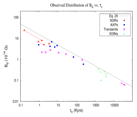
Figure 2: Inferred Dipole Field ($B_{\rm dip}=3.2\times 10^{19}\sqrt{P\dot{P}}\;$G) vs. characteristic spindown age ($\tau_{\rm c}=(1/2)P/\dot{P}$) for SGRs, AXPs, transients and XDINs. The dashed line in Fig. 2 represents the scaling of Eq. (20), expected from field decay with $\alpha<2$, using $P_{\infty}=11.77\;$s that corresponds to the longest measured spin period (for AXP 1841-045). The magenta arrow indicates the current upper limit on the position of SGR 0418+5829. The red triangles joined by dotted lines represent the whole range of values spanned by SGR 1806-20 and SGR 1900+14, as explained in the text (cfr. Tab. 1).

We begin by assessing whether the distribution of dipole magnetic fields of magnetar candidates, as inferred from timing observations, can provide indications for field decay. Fig. 2 shows the inferred dipole fields, $B_{\rm dip}$, of magnetar candidates plotted versus their spindown age, $\tau_{c}$. This represents an alternative projection of the usual $P-\dot{P}$ diagram.

Two points stem most clearly from Fig. 2. First, the absence of old objects (with relatively large spin-down ages) with strong dipole fields and the tendency for objects with increasingly stronger fields to be found only at increasingly younger spin-down ages. The dashed line in Fig. 2 represents the scaling of Eq. (20), expected from field decay with $\alpha<2$, using $P_{\infty}=11.77\;$s that corresponds to the longest measured spin period (for AXP 1841-045). The apparently prohibited region in parameter space is equivalent to the existence of a limiting spin period for the objects considered. As discussed in previous sections, precisely such an asymptotic spin period is expected if the dipole field decays and its decay is governed by a physical mechanism with $\alpha<2$.

Second, all “old” sources (spin-down age $\tau_{c}\gtrsim 10\;$kyr) lie in a narrow strip corresponding to $3.5\;{\rm s}\lesssim P_{\infty}\lesssim 11\;$s, i.e. within a factor of $\approx 3$ in their spin period. In the context of magnetic field decay models, the fact that this strip is so narrow can be interpreted in one of two ways. Either (1) all “old” AXPs, XDINs and SGR0418+5729 came from a narrow distribution of initial dipole fields $B_{\rm dip,i}$, in which case a relatively large range of $\alpha<2$ values would be compatible with observations, or (2) $\alpha$ is sufficiently close to 2 that field decay has largely washed out the spread in $B_{\rm dip,i}$ values, which could have been significantly larger in this case.

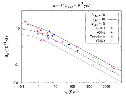
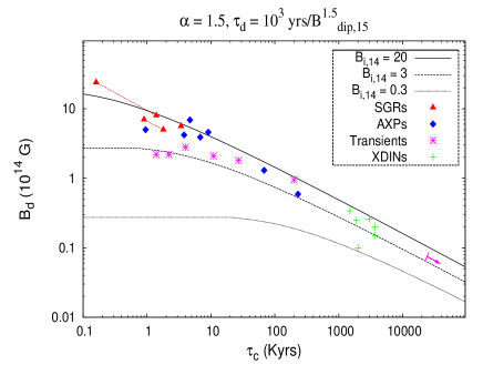
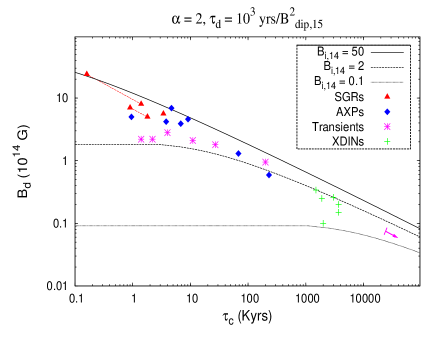
Figure 3: Different models of field decay with asymptotic spin period, ($\alpha<2$) compared with the inferred dipole values of magnetar candidates from timing measurements. The magenta arrow represents the current upper limit to the position of SGR 0418+5729. The plotted curves don’t represent fits to data but the normalization of the decay timescale ($A$) was chosen, for each value of $\alpha$, to match the position of sources.

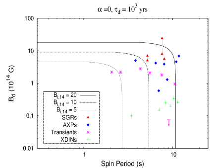
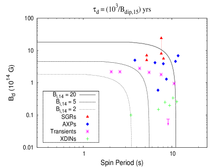
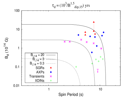
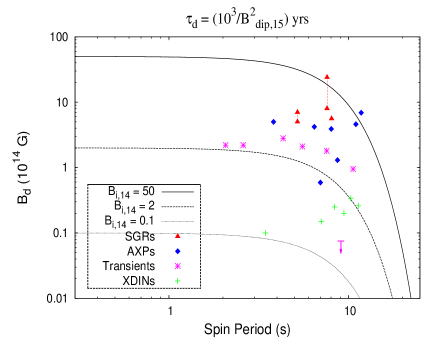
Figure 4: Different models of field decay with asymptotic spin period ($\alpha<2$) in the $B_{\rm dip}$ vs. P plane. The magenta arrow indicates the current upper limit to the position of SGR 0418+5729. The curves correspond to the same models of the previous figure.

The distribution of sources shown in Fig. 2 can be understood as follows. For young objects, $t\ll\tau_{\rm d,i}$, the magnetic field does not have time to decay and it is almost constant. This implies a constant $\dot{B}$ and a constant $\dot{E}_{B_{\rm dip}}\propto B_{\rm dip}^{2+\alpha}$. At this stage the period $P$ and the spin-down age grow while the dipole field $B_{\rm dip}$ doesn’t vary (corresponding to a horizontal trajectory in the $B_{\rm dip}\,$–$\,\tau_{c}$ plane). Moreover, the object has a nearly constant power output due to magnetic field decay up to $\tau_{\rm c}\lesssim\tau_{\rm d,i}$, at which point the power drops following the decay of the magnetic field. This evolution scenario implies that objects with age $t\leq\tau_{\rm d,i}$ are most likely to be detected close to $\tau_{\rm d,i}$ since, for a constant power output, they spend more time at $\tau_{\rm c}\sim\tau_{\rm d,i}$.

This is particularly expected for SGRs, since they are detected predominantly through their bursting activity, which is thought to be directly powered by the decay of their magnetic field, rather than through their quiescent emission (which might have a non-negligible contribution from the NS residual heat). Therefore, the fact that we do not detect any SGRs with magnetic fields of several $\times 10^{14}\;$G but larger spin periods ($P\gg 10\;$s), strongly supports a decay of the dipole field on a timescale of $\tau_{\rm d,i}\approx 10^{3}(B_{\rm dip,i}/10^{15}\,{\rm G})^{-2}\;$yr, in these objects. Note that, if the SGR’s magnetic dipole field did not decay on such a timescale, a large population of SGRs with spin periods of tens or even hundreds of seconds would exist. Such large period SGRs should be easy to detect if they maintained similar magnetic fields and thus similar bursting activity as the observed SGR sample. Even objects with much weaker or no bursting activity but larger spin-down ages are detected (e.g., AXPs, transients, XDINs) which, if there was no magnetic field decay, would imply similarly larger ages. Therefore, we find it highly unlikely that long period SGRs, with $P\gg 10\;$s, exist in much larger numbers than the observed SGR sample but are not detected for some unknown reason.

Objects with ages $t\ll\tau_{\rm d,i}$, which populate the lower-left region of the $B_{\rm d}\,$–$\,\tau_{c}$ plane, are detected with proportionally smaller probability, unless their bursting/flaring activity is stronger at younger ages, resulting in a greater detectability that could compensate for the short time spend in this part of the diagram. Relatively old objects with an age $t\gg\tau_{\rm d,i}$ will have reached their asymptotic period $P_{\infty}$ (for $\alpha<2$) and will thus be found on the asymptotic line, $B_{\rm d}\propto\tau^{-1/2}_{c}$. These will have a much lower luminosity than their younger brethren and will be detected only if, e.g., they are sufficiently close to us or if they maintain some level of bursting activity.

Finally, we note that 5 out of 7 transient SGRs/AXPs lie, in the $B_{\rm dip}$ vs. $\tau_{c}$ diagram, below the asymptotic line. This suggests that $\tau_{\rm c}$ is not much longer than their $\tau_{\rm d,i}$. CXO J164710.2-455216 and, of course, of SGR 0418+5729 represent two notable exceptions, as both appear to lie well on the asymptotic line (hence, $\tau_{\rm c}>\tau_{\rm d,i}$). In particular, the former object has both $\tau_{\rm c}$ and $B_{\rm dip}$ comparable to the persistent AXP 1E2259+586.

We summarize the effect of field decay in Figs. 3 and 4. We also show in Fig. 5 the corresponding tracks in the usual $P$-$\dot{P}$ diagram. As already stated, previous plots just represent different projections of these fundamental measured quantities.

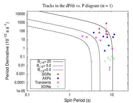
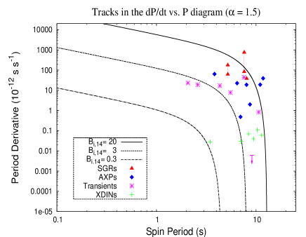
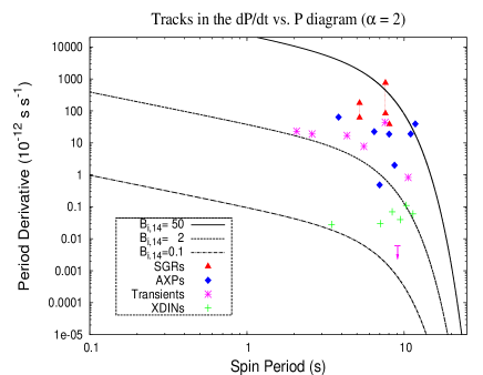
Figure 5: Tracks in the $\dot{P}$ vs. $P$ plane expected for the different cases of field decay previously discussed, compared to measured source positions. Plotted curves do not represent fits to data. Different symbols and lines are as in previous figures.

We can estimate a minimal spread in $B_{\rm dip,i}$ from Fig. 2 by restricting attention to objects lying well below the asymptotic line, so that $\tau_{\rm c}<\tau_{\rm d,i}$. The strongest value of the field is $8\times 10^{14}$ G in SGR 1806-20, while the weakest is $1.8\times 10^{14}$ G in SGR 1833-0832. These numbers imply a minimal spread $\approx 4.5$ for the initial field distribution of the whole population.

For a given value of $\alpha<2$ (and a fixed normalization $A$), Eq. (11) can be used to derive a general relation between the observed spread in $P_{\infty}$ at late times and the initial spread in $B_{\rm dip,i}$ that produced it. For a distribution of initial dipoles in the range $B_{\rm i,min}<B_{\rm dip,i}<B_{\rm i,max}$ (or $1<B_{\rm dip,i}/B_{\rm i,min}<\Delta_{B}\equiv B_{\rm i,max}/B_{\rm i,min}$) a spread $P_{\infty,{\rm min}}<P_{\infty}<P_{\infty,{\rm max}}$ (or $1<P_{\infty}/P_{\infty,{\rm min}}<\Delta_{P}\equiv P_{\infty,{\rm max}}/P_{\infty,{\rm min}}$) is expected. Therefore

$$\Delta_{B}=\Delta_{P}^{2/(2-\alpha)}\quad\Longleftrightarrow\quad\log\Delta_{P}\equiv\log\left(\frac{P_{\infty,{\rm max}}}{P_{\infty,{\rm min}}}\right)=\frac{2-\alpha}{2}\log\left(\frac{B_{\rm i,max}}{B_{\rm i,min}}\right)\equiv\frac{2-\alpha}{2}\log\Delta_{B}\ .$$ (26)

In order to quantify $\Delta_{P}$ from the data, we evaluate the average spin period, $\langle P\rangle$, and standard deviation, $\sigma_{\rm P}$, of those sources which are old enough to be considered close to the asymptotic line, e.g. having $\tau_{\rm c}\geq 10^{4}$ yrs. The resulting subsample contains 13 sources, with $\langle P\rangle\approx 8.42$ s and $\sigma_{\rm P}\approx 2.2$ s. The parent population would thus be characterized by a $2\sigma$ spread of $\simeq 3.3$, corresponding to the ratio between the slowest and fastest spinning objects of the subsample. We plot relation (26) in the left panel of Fig. 6, where the two curves correspond to the 1$\sigma$ and $2\sigma$ values of $\Delta_{P}$, as derived above.

A totally independent constraint on $\alpha$ can be derived considering the very weak, thermal, X-ray emission of SGR 0418+5729. In relative quiescence (on 2010 July 23rd, Rea et al. (2010)) this is dominated by a black-body component with a temperature of $kT=0.67\pm 0.11\;$keV, and corresponding 0.5 –$\,10\;$keV luminosity, $L_{\rm X}\sim 6.2\times 10^{31}\;{\rm erg\;s^{-1}}$ In the earlier, more active period (June to November 2009), the temperature gradually decreased from $kT\approx 1.0\;$keV to $\approx 0.8\;$keV and $L_{X}$ was between one and two orders of magnitude higher (Esposito et al., 2010), while the corresponding emitting areas gradually decreased. This suggests that even this weak X-ray emission is more likely to originate from a localized heating event associated to the recent bursting activity, rather than being powered by the secular cooling of the NS. Hence, the luminosity of $6\times 10^{31}\;{\rm erg\;s^{-1}}$ can be considered as a solid upper limit to the quiescent X-ray emission of this object. This value compares well with the X-ray luminosity of $\sim 10^{5}$ yr-old, passively cooling objects, like B0656+14 (Yakovlev & Pethick, 2004), while younger $10^{3}\,$–$\,10^{4}\;$yr old isolated, passively cooling NSs are at least one order of magnitude brighter than the upper limit for SGR 4018+5729. Since field decay is likely to provide additional heat in the latter object, the age of B0656+14 represent as a robust lower limit to the true age of SGR 0418+5729.

In the right panel of Fig. 6 we plot the estimated age of SGR 0418+5729 as a function of $\alpha$, for the whole range of values that give an asymptotic spin period ($0\leq\alpha<2$). The line corresponding to the above lower limit, $10^{5}\;$yr, is drawn for clarity. Note that as $\alpha$ approaches 2 from below the true age of SGR 0418+5729 becomes progressively closer to its spindown age.

Combining the constraints from these two figures, we can rule out, or at least to consider very unlikely, values of $\alpha\lesssim 1$. Combined with the earlier constrains this implies $1\lesssim\alpha<2$.

The points discussed above are illustrated quantitatively in Fig. 3, where trajectories in the $B_{\rm dip}\,$–$\,\tau_{c}$ plane are plotted for different values of $\alpha$ and for a given initial distribution of dipole fields, $B_{\rm dip,i}$, comparing them to the objects in our sample. Fig. 4 shows trajectories in the $B_{\rm dip}\,$–$\,P$ plane for the same sources, same field decay models and $B_{\rm dip,i}$ distributions as Fig. 3. This represents an alternative way of illustrating the same argument. Below we draw some conclusions from these plots regarding the viability of different $\alpha$ values.

Exponential decay ($\alpha=0$) can explain the observed distribution of sources in the $B_{\rm dip}\,$–$\,\tau_{c}$ or $B_{\rm dip}\,$–$\,P$ planes if the field decay timescale is particularly short, $\tau_{\rm d}=\tau_{\rm d,i}\approx 1\;$kyr. Longer timescales would fail to halt the spindown at sufficiently short spin period, so this is quite a strict requirement. This model could work if all the sources considered here came from a very narrow distribution of initial dipole fields (as can be seen in Figs. 3 and 4). In particular, Fig. 4 shows that even a factor 4 spread in $B_{\rm dip,i}$ would lead to a significantly wider distribution of spin periods than observed (i.e a factor of 4 spread in $P_{\infty}$ compared to the observed factor of $\lesssim 3$). Indeed, Eq. (11) shows that the value of $P_{\infty}$ is linear in the initial field, $B_{\rm d,i}$, for $\alpha=0$.

Given the short timescale required by the exponential decay, the implied age of SGR0418+5729 would have to be younger than, at most, $5\;$kyr, as can be derived from Eq. (15). This is in sharp contrast with the minimal age that we derived for SGR 0418+5729 based on its weak thermal emission. Additionally, the age of SGR 0418+5729 would not be much larger than that of other transients with much smaller $\tau_{\rm c}$, while its X-ray emission would be a factor 10-50 lower. Explaining such a fast decrease in $L_{\rm X}$ at these young ages would also represent a major challenge. Overall, exponential decay of the field appears ruled out based on the very weak emission of SGR 0418+5729.

The case $\alpha=1$ provides a reasonable description of the distribution of sources in Fig. 3 and Fig. 4. Although this case suggests a straightforward relation to the basic Hall decay mode (cfr. sec. 4), note that the curves in Fig. 3 and 4 were drawn by adjusting the normalization of the decay timescale, $A$, to be 10 times smaller than the value provided by Cumming et al. (2004) and GR92. Namely, we assumed

$$\tau_{\rm d}\simeq\frac{10^{3}}{B_{\rm dip,15}}{\rm yrs}$$ (27)

The decay for sources whose initial field was larger than $\simeq 2\times 10^{14}$ G would be to slow with the Hall decay time of Eq. 25 and in this case most AXPs/SGRs would evolve to significantly longer spin periods at later times. These older counterparts would occupy a region right above XDINS and SGR0418+5729 in the $(\tau_{c},B)$ plane (Fig. 2) where no object is actually found. Note, however, that the timescale of Eq. 25 could match our empirical scaling if the decay of Hall modes were regulated by processes occurring at somewhat lower crustal densities, $\lesssim 3\times 10^{13}$ g cm^-3, well above the crust/core interface.

This model for field decay implies that all sources come from a distribution of initial dipoles in the range $(0.2-2)\times 10^{15}$ G, although most of them (20 out of 23) were between $5\times 10^{14}$ G and $2\times 10^{15}$ G. The XDIN RX J0420 would represent a notable exception, having reached a remarkably short asymptotic spin period of $\approx 3.45$ s because its initial dipole was weaker. The two transients 1E 1547-5408 and SGR 1627-41, which are slightly below the range of the other 20 objects, would also populate the weak-field tail of the distribution of $B_{\rm dip,i}$.

Overall, this scenario appears to account well for the observed distribution of sources, although a full self-consistent population synthesis model is needed to verify this quantitatively.

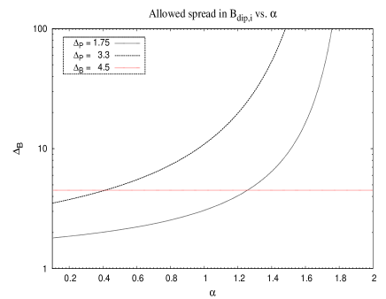
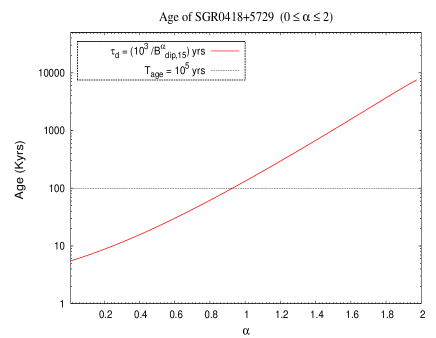
Figure 6: Constraints on the value of $\alpha$. Left Panel : The allowed spread in the initial magnetic field distribution as a function of $\alpha$, for 3 different values of the spread in asymtpotic spin period. Right Panel : The inferred age of SRG 0418+5729, as a function of the chosen value of $\alpha$. The likely lower limit $\sim 10^{5}$ yrs to the age of this source is drawn as a horizontal line.

Phenomenological decay law with intermediate value of $1<\alpha<2$ (e.g. $\alpha\approx 1.5$). Although there are no existing models for field decay predicting $1<\alpha<2$, we choose this particular value of $\alpha$ as representative of cases in which a wider spread in $B_{\rm dip,i}$ ($\Delta_{B}\gg 1$) is allowed, despite the observed modest spread in $P_{\infty}$ ($\Delta_{P}\approx 3$).

Fig. 3 shows $B_{\rm dip}$ vs. $\tau_{c}$ trajectories with this choice of $\alpha$. One can see that these converge to a narrow strip despite an initial wide distribution of $B_{\rm dip,i}$. This scenario can well reproduce also the distribution of sources in the $B_{\rm dip}\,$–$\,P$ plane, including the apparent absence of spin periods longer than $\simeq 12$ s. Note that the normalization for the decay timescale, $\tau_{\rm d,i}=10^{3}\;$yr for $B_{\rm dip,i}=10^{15}\;{\rm G}$, was chosen to match the scaling of Eq. 20, represented by the dashed line in Fig. 2.

An effective power-law decay with index $\approx 1.5-1.8$ is expected in the ohmic decay model by Urpin, Chanmugam & Sang (1994). This is not completely equivalent to our phenomenological decay law, though, since in that model the ratio $B_{\rm dip}(t)/B_{\rm dip,i}$ is still a universal function, determined by the field-independent parameter $\tau_{\rm d,i}$. In particular, this implies a linear relation between $P_{\infty}$ and $B_{\rm dip,i}$. Thus, in order for the asymptotic spins of our sources to all fall in the observed narrow range, a correspondingly narrow range in ${\rm B}_{\rm dip,i}$ is required. This is the same problem as in the $\alpha=0$ case. To circumvent it, one has to assume that $\tau_{\rm d,i}$, the initial decay time, is itself a function of $B_{\rm dip,i}$. This extra assumption would make the crustal decay model totally equivalent to our phenomenological model. Since $\tau_{\rm d,i}$ is determined by the initial location of the electric currents that sustain the field, a strict (anti)correlation between the initial field strength and the initial depth at which currents flow is implied. This is far from trivial and an account of its implications is left for future study.

The limiting case, $\alpha=2$ is shown for the sake of completeness. As the previous case, it provides a narrow range of asymptotic spin periods, even starting from a very wide distribution of initial magnetic field values. However, as already discussed, it does not have an actual asymptotic spin period, which implies that spin periods of order 20 s would be expected in older objects. Thus, this case is disfavored by the data compared to $\alpha\approx 1.5$. Also in this case, the normalization for the decay timescale was chosen arbitrarily as above.

It is also possible that two different mechanisms for field decay operate, respectively above or below some threshold value of the dipole field, $B_{*}$. We refer to these as the early and late mechanism for field decay, according to the time when they dominate, and denote their decay index as $\alpha_{e}$ or $\alpha$, respectively. At each value of $B_{\rm dip}$ the mechanism with the shorter decay time $\tau_{\rm d}$ determines the overall field decay and, of course, the two times are equal at $B_{*}$, with the value $\tau_{*}$.

In such a scenario, a wide distribution of $B_{\rm dip,i}$ at birth can also result in a narrow distribution of $P_{\infty}$. As such, it is only meaningful for $\alpha$ much below 2 (say $\alpha=1$) and $\alpha_{e}$ significantly larger than 2. Sources with $B_{\rm dip}>B_{*}$ would initially evolve along a shallow trajectory, $\propto(t/\tau_{\rm d,i})^{-1/\alpha_{e}}$ in the $B_{\rm dip}\,$–$\,\tau_{\rm c}$ plane. Because $\alpha_{e}>2$, trajectories for different initial fields would converge to a narrow bundle of curves while $\tau_{\rm c}<\tau_{*}$. Upon reaching the point where $\tau_{\rm c}=\tau_{*}$ they would then meet the line corresponding to the late mechanism ($\alpha<2$) and follow that beyond $\tau_{*}$.

Applying this reasoning to Fig. 2 we derive the values of $B_{*}\sim 6.9\times 10^{14}\;$G and $\tau_{*}\sim 4.5\;$kyr, corresponding to the position of the AXP 1E 1841-045. However, only SGR 1806-20 is above this threshold, implying that the early mechanism could still be dominant only in it. Stated differently, in all the observed sources - but one at most - invoking a second, early decay mechanism doesn’t help to reduce the initial spread in $B_{\rm dip,i}$.

6 The persistent X-ray luminosity

Having assessed the decay of the dipole field in magnetar candidates, we now turn to test whether such a decay can account for their observed X-ray luminosity, $L_{X}$, which typically exceeds their spin-down power, $|\dot{E}_{\rm rot}|$.

We define the magnetic luminosity of the dipole field, $L_{\rm B,dip}\equiv 2E_{\rm dip}/\tau_{\rm d}$, as the available power of a dipole field decaying on the timescale $\tau_{\rm d}$. Here, the total energy of the field is $E_{\rm dip}=(4\pi R_{*}^{3}/3)B_{\rm dip}^{2}/(8\pi)=R_{*}^{3}B_{\rm dip}^{2}/6\simeq 1.7\times 10^{47}B^{2}_{\rm dip,15}R^{3}_{*,6}\;$erg and, following the definition of Eq. (7):

$$L_{\rm B,dip}=-\frac{dE_{\rm dip}}{dt}=-\frac{R^{3}_{*}}{6}\frac{d(B^{2}_{\rm dip})}{dt}=\frac{R^{3}_{*}B^{2}_{\rm dip}}{3\tau_{\rm d}}=\frac{2E_{\rm dip}}{\tau_{\rm d}}\simeq 5.3\times 10^{36}B^{2}_{\rm dip,15}R^{3}_{*,6}\tau_{\rm d,kyr}^{-1}\;{\rm erg\;s^{-1}}\ .$$ (28)

Fig. 7 depicts a comparision of the total available magnetic power for the same four field decay models examined in sec. 5 with the observed X-ray emission of SGRs, AXPs, transients and XDINs. The three main groups of sources (SGRs/AXPs, transients and XDINs) populate three separate regions in parameter space and in the following we comment on them separately. We focus, first, on the persistent AXPs/SGRs, for which results and conclusions are much clearer, and comment later on the more problematic XDINs and transients.

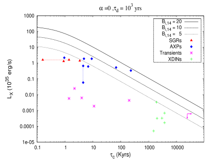
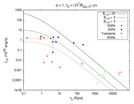
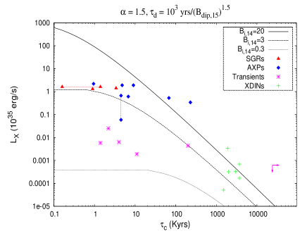
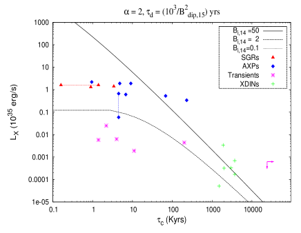
Figure 7: A comparison of the maximal bolometric luminosity as a function of $\tau_{\rm c}$ expected from the decay of the dipole field, according to the models of section 5, with the observed X-ray luminosity of different classes of magnetars. The magenta arrows indicate current upper limits to the spindown age and $L_{\rm X}$ of SGR 0418+5729.

6.1 Persistent SGRs, AXPs and SGR 0418+5729

Overall, the evolution of $L_{\rm B,dip}$ with $\tau_{\rm c}$ as derived from the above models for field decay does not match well the distribution of sources in parameter space. In particular, relatively old sources ($\tau_{\rm c}\geq 10^{5}$ yrs) tend to be more luminous, in the 2 – 10 keV energy range, than the maximum available power from decay of the dipole field namely, $L_{X}>L_{\rm B,dip}$. These old sources thus provide the strongest indication that even the decay of their dipole field is not able to explain the X-ray luminosity.

An exponential decay with $\alpha=0$ and with a short $\tau_{d}$ appears consistent with all observations. However, as previously discussed, an exponential field decay on a $\sim 1\;$kyr timescale would imply an implausibly young age ($\leq 5\times 10^{3}$ yrs) for SGR 0418+5729 and would require a very narrow initial magnetic field distribution. On these grounds, exponential decay of the field is discarded anyway.

Decay with $\alpha=1$ falls short of the observed emission of the two AXPs with $\tau_{\rm c}\gtrsim 10^{5}\;$yr. Although the mismatch is apparently by a small factor, we stress that curves represent the total available magnetic power, while data points include only the observed emission in the 2 – 10 keV energy range. The bolometric luminosity is a few times larger. Gravitational redshift also introduces a non-negligible correction to the observed luminosity (see sec. 7.1). Finally, the radiative efficiency may well be less than unity since field decay is also expected to dissipate energy in other channels (such as neutrino emission or bursting activity). The presence of two AXPs beyond the upper curve must therefore be considered as a significant failure of this model.

For $\alpha=1$, the observed X- ray luminosity of SGR 0418+5729 is 30 times larger than the available power from dipole field decay, according to Eq. 28. Although, as discussed in section §2, this may overestimate the quiescent power, we don’t expect the average power output to be lower by more than a factor of 10 than that and, even with this correction, the dipole energy is still insufficient.

For values of $\alpha>1$ the mismatch between curves and observations is striking. The distribution of persistent sources in the $L_{\rm X}\,$–$\,\tau_{\rm c}$ plane is at best marginally consistent with being powered by the decay of the dipole field, if $\alpha=1$, while it is totally inconsistent for larger values of $\alpha$. In general, the X-ray luminosity appears to decay on a longer timescale, and to be associated with a larger energy reservoir, than can be provided by the decaying dipole fields. Sources are indeed found at a fairly constant level of X-ray luminosity up to $\tau_{\rm c}\sim 10\;$kyr. The few older objects known clearly show a decline of $L_{\rm X}$ with (spindown) age which, however, is flatter than expected from the decay of the dipole field.

In the framework of the magnetar model, the most natural explanation for these findings is that the persistent X-ray emission of these sources is powered by the decay of an even larger field component, stored in their interior In the next section we try to assess the location of such a (presumably magnetic) energy reservoir and its most likely decay modes.

6.2 X-ray Dim Isolated Neutron Stars

The thermal X-ray luminosity of XDINs is much dimmer than that of persistent magnetar candidates. It is even possible, in principle, to explain it within the so-called “minimal cooling” scenario for passively cooling NSs. However, it is difficult to reconcile the relatively bright emission of RXJ 0720 with its apparent old age ($\sim 2\times 10^{6}\;$yr) within that scenario. This suggests a possible role of strong internal heating in this object (Page et al., 2004). On the other hand, the possibility of mild internal heating in most XDINs has also been recently suggested, based on a tendency for their effective temperatures to be higher than that of normal pulsars with the same age (Kaplan & van Kerkwijk, 2011).

From Fig. 2 we conclude that XDINs should be interpreted as objects whose dipole field has decayed substantially, hence their true ages must be younger than their spin-down ages, which are narrowly clustered around $\tau_{\rm c}\sim{~{}\rm a~{}few~{}}\times 10^{6}\;$yr. This favors passive cooling models in accounting for the effective temperatures and X-ray luminosities of XDINs, possibly removing the need for internal heating in all these sources. On the other hand, for $\alpha=1$ the energy released by the dipole field decay is not negligible compared with their X-ray luminosities (see Fig. 7). Whether this can significantly affect their temperatures as compared to normal pulsars can only be checked through detailed cooling modeling, which are beyond the scope of this work.

If, however, detailed modeling will reveal that these luminosities are too large for passive cooling then we have to consider heating sources. RXJ 0720 stands here as a unique object. Even with $\alpha=1$, Eq. 28 yields $L_{\rm B,dip}\approx 8\times 10^{31}~{}{\rm erg~{}s}^{-1}$ , which is a factor $\sim 5$ lower than its measured $L_{X}$. This could not be explained by $L_{\rm B,dip}$ and would thus hint to the presence of an additional energy reservoir, siimilar to magnetar candidates. In this case, some level of bursting activity would accordingly be expected from this source. For $\alpha>1$, the available $L_{\rm B,dip}$ is insufficient even to account for the X-ray luminosity of RXJ 2143 and it is marginal compared with other XDINs.

We conclude that the decay of their dipole field implies that XDINs are younger than their spindown age, $\tau_{\rm c}$, which could improve the match between cooling models and their X-ray emission properties. On the other hand, there is no compelling evidence for a dominant contribution to their X-ray emission from the decay of the dipole field. The case $\alpha=1$ is, at most, marginally consistent with this hypothesis while, as $\alpha$ becomes $>1$, it is increasingly hard for $L_{\rm B,dip}$ to match the observed $L_{\rm X}$.

We can use the observed emission properties of XDINs to further constrain the possible values of $\alpha$. It was recently shown that the spindown ages of XDINs are systematically longer, by a factor $\sim$ 10, than the ages of NSs with similar effective temperatures (Kaplan & van Kerkwijk, 2011). The simplest intepretation of this fact is that, due to dipole field deacy, their $\tau_{\rm c}$ overestimate their true ages by approximately one order of magnitude. We can compare quantitatively this statement with models for decay of the dipole field. For a given value of $\alpha$, the formulae of § 5 allow to derive the value of $B_{\rm dip,i}$ corresponding to each individual XDIN from its $\tau_{\rm c}$ and $B_{\rm dip}$ (or equivalently, $P$ and $\dot{P}$) and, from its $\tau_{\rm c}$, obtain its real age, $t_{\rm age}$. These estimates, for the cases $\alpha=1$ and $\alpha=1.5$, are summarized in Table 2. For the sake of completeness, we report in the last column of this table the effective temperature, $kT_{\rm eff}$, for each source, as derived by the spectral fits.

	$\tau_{\rm c}$ [kyr]	$t_{\rm age}$ [kyr]	$t_{\rm age}$ [kyr]	$kT_{\rm eff}$ [eV]
Name		($\alpha=1$)	($\alpha=1.5$)
RXJ 1308	1500	30	100	102
RXJ 0806	3000	40	160	96
RXJ 0720	1900	42	160	90
RXJ 2143	3700	50	200	100
RXJ 1856	3700	66	350	63
RXJ 0420	2000	100	580	44

Table 2: Spindown age, true age (for two different values of the decay index, $\alpha$) and effetive temperature of the six XDINs considered in this work.

Note that the derived age distributions match fairly well the distribution of effective temperatures, as opposed to the $\tau_{\rm c}$ distribution. It is clear, however, that low $\alpha$ values give corrections to the spindown ages of XDINs by a factor $\lesssim$ a hundred, which it too large. The case $\alpha=1.5$, on the other hand, gives just the right correction factors of order ten.

Finally we note the striking clustering of XDINs at $\tau_{\rm c}\in[1.5-3.7]$ Myr. Together with their comparatively wider spread in X-ray luminosities, $[\lesssim 10^{31}-3\times 10^{32}]$ erg s^-1, it suggests that these sources may have reached some threshold age, at which cooling becomes very efficient, the luminosity drops sharply and the sources become undetectable. This can happen, for example ,if the sources enter the photon-cooling dominated regime (Page et al. (2004) and references therein). In this framework, the actual age of XDINs should be just slightly larger than the time at which the transition to photon-cooling occurs.

From Tab. 2 we see that, for $\alpha=1$, all XDINs would have ages $\leq 10^{5}$ yr, most of them being significantly younger than that. In this case, a transition to photon-cooling at $t_{\rm age}<3\times 10^{4}$ yrs would have to be invoked, however, in most “standard” cooling models this transition occurs at $\gtrsim 10^{5}\;$yr (Yakovlev & Pethick, 2004; Page et al., 2004). Only the fastest cooling models have this transition at $\sim 3\times 10^{4}\;$yr (Page et al., 2004, 2011) and are thus just marginally consistent. Even in this case, however, the weak X-ray emission of XDINs at such young ages would represent by itself a major problem. No cooling model predicts X-ray luminosities $<10^{32}$ erg s^-1 at ages $t_{\rm age}<10^{5}$ yrs. As a conclusion, the case $\alpha=1$ is clearly very problematic from this point of view.

For $\alpha=1.5$, on the other hand, all ages are $\sim[1-{\rm a~{}few}]\times 10^{5}$ yrs. This allows an easier interpretation of the XDINs as cooling NSs having just passed the transition to photon-cooling, the older ones being progressively cooler and dimmer.

The observed properties of XDINs thus strongly argue against a value of $\alpha=1$ and are much more consistent with $1.5\lesssim\alpha<2$. In particular, the value $\alpha\approx 1.5$ provides an overall good agreement with the main observed properties of these sources. Altogether, taking into account the requirement of $\alpha$ sufficiently below $2$ to account for lack of periods well above 10 s, we conclude that $1.5\lesssim\alpha\lesssim 1.8$ is strongly favored by the data.

6.3 Transients

Transient AXPs are the most enigmatic objects. Most of them appear to be young sources whose field has not significantly decayed yet and their weak quiescent emission testifies of an extremely low efficiency in converting magnetic energy into X-rays. This could be related to magnetic dissipation (heat release) occurring only deep in the NS core, involving only a fraction of the whole volume and resulting in large neutrino energy losses and a low efficiency for the X-ray emission. As opposed to this, magnetic dissipation would be more distributed, or would occur closer to the NS surface, in persistent sources, thus reducing neutrino losses and leading to a higher efficiency of the X-ray emission. However, during outbursts transients become temporarily very similar to the persistent sources and get much closer to them in the $L_{\rm X}\,$–$\,\tau_{\rm c}$ plane. The origin of this behaviour is still unclear and we will not discuss it further.

7 Decay of the internal magnetic field

The presence of internal fields larger than the dipole components in magnetars has been considered as a likely theoretical possibility since the suggestion made by TD96. In the previous sections we have provided, for the first time, evidence based on the observed properties of persistent SGRs/AXPs that such a component must exist, if magnetic energy is indeed powering their X-ray emission.

The decay of the internal field is even harder to constrain than the dipole, as the only observational guidance is the evolution of $L_{\rm X}$ and the level of bursting activity (the latter being more qualitative in nature as it is harder to accurately quantify it). The X-ray luminosity depends on several physical details of the NS structure other than the properties of field decay. To keep the focus on the salient effect, we adopt a different approach here and, instead of dealing with general phenomenological decay models, we will calculate the expected evolution of $L_{\rm X}$ with $\tau_{\rm c}$ adopting two simple and general prescriptions from selected, physically-motivated models of field decay in NS interiors.

There are two main possible locations for the decay of the internal field. It could either take place in the liquid core of the NS, at $10^{14}\lesssim\rho<10^{15}$ g cm^-3 (TD96, Heyl & Kulkarni 1998; Thompson & Duncan 2001; Colpi et al. 2000; Arras et al. 2004; Dall’Osso et al. 2009), or in the rigid lattice of the inner crust, at $\rho\lesssim 10^{14}$ g cm^-3 (Vainshtein et al., 2000; Konenkov & Geppert, 2001; Arras et al., 2004; Pons & Geppert, 2007; Pons et al., 2009). In either case, heat released locally by field dissipation is subsequently conducted to the surface, thereby powering the enhanced X-ray emisson. Note that energy release may also take place at the NS surface, or just below it ($\rho\lesssim 10^{10}$ g cm^-3, Kaminker et al. 2009, e.g. due to a gradual dissipation of electrical currents in a global/localized magnetospheric twist (Thompson et al., 2002; Beloborodov & Thompson, 2007; Beloborodov, 2009). This would likely allow a larger radiative efficiency. However, the twist and associated radiation would still draw their energy from that of an evolving, strongly twisted internal field, either in the deep crust or core.

As far as field decay in the liquid core is concerned, the state of matter there plays an important role. If it is normal $npe$ matter, as opposed to superfluid, then ambipolar diffusion is expected to be the dominant channel through which the magnetic field decays. If, instead, either protons or neutrons (or both species) were in a condensed state, particle interactions may be significantly affected, reducing or possibly quenching the mode (GR92, Thompson & Duncan 1996; Jones 2006; Glampedakis et al. 2011). We do not discuss the role of core condensation. Here we note that, even if ambipolar diffusion were completely quenched by core condensation, field decay in the crust, driven by the Hall effect, would still continue unaffected by the changing conditions in the core (Arras et al. (2004) give a quantitative account of this).

Therefore, with the aim of illustrating just the salient effects on the X-ray luminosity of the decay of a strong internal field, we will consider here only the two limiting cases: ambipolar diffusion in a normal core of $npe$ matter, or Hall-driven field decay in the inner crust, with a magnetically inactive core. The latter could be considered as a “minimal heating scenario” for magnetars. A study of realistic models, which include the contribution to field dissipation of hydromagnetic instabilities (Arras et al., 2004) and magnetospheric currents (Thompson et al., 2002; Beloborodov & Thompson, 2007), along with the effects of strong crustal magnetic fields and light-element envelopes/atmospheres on radiative transfer, is clearly beyond the scope of this work.

7.1 Field decay in the NS core

We consider evolution of the internal field ($B_{\rm int}$) through the solenoidal mode only. In addition to previous treatments (Heyl & Kulkarni, 1998; Colpi et al., 2000; Arras et al., 2004), we allow explicitly for a different decay law for the dipole field, according to our conclusions of sec. 5 and sec. 6. In our picture the decay of $B_{\rm int}$ heats the core and powers the surface X-ray emission, which will then decline following the decrease of the internal field. The decay of the dipole field will, on the other hand, determine the relation between real time, $t$, and spindown age, $\tau_{\rm c}$ (see Fig. 1). We restrict attention to the two more realistic cases, $\alpha=1$ or $1.5$, as emerged in previous sections.

For a core of normal $npe$ matter the decay time for the solenoidal mode of ambipolar diffusion is $\tau_{\rm d,int}\approx 10^{4}/B^{6/5}_{\rm int,16}$ yrs. The total available magnetic luminosity is then, according to Eq. 28, $L_{\rm B,int}=(R^{3}_{*}/3)B^{2}_{\rm int}/\tau_{\rm d,int}\approx 10^{38}B^{16/5}_{\rm int,16}R^{3}_{*,6}{\rm erg\ s}^{-1}$.

As discussed in sec. 4, the equilibrium between heating and neutrino cooling determines the temperature as a function of $B_{\rm int}$, when ambipolar diffusion is active, as expressed by Eq. 4. The evolution of the core temperature, $T_{\rm c}$, will thus track directly that of $B_{\rm int}$.

Finally, an appropriate relation between the core and surface temperatures is needed in order to calculate the expected surface X-ray emission. This is the so-called $T_{\rm b}-T_{\rm s}$ relation, where $T_{\rm b}$ is the temperature at the base of the crust, the core being isothermal due to its large density and heat conduction. We adopt the minimal scaling for an unmagnetized, Fe envelope (Potekhin & Yakovlev 2001)

$$T_{\rm s}\simeq 1.17\times 10^{6}~{}{\rm K}~{}\left[(7\zeta)^{9/4}+\left(\frac{\zeta}{3}\right)^{5/4}\right]^{1/4}$$ (29)

where $\zeta\equiv T_{\rm c,9}-0.001~{}g^{1/4}_{14}(7~{}T_{\rm c,9})^{1/2}$ and $g_{14}\approx 1.87$ is the surface gravity.

The above relation is known to be sensitive to the strength and topology of crustal magnetic fields (Page, Geppert & Küker, 2007; Kaminker et al., 2009; Pons et al., 2009) and also to the chemical composition of the outer layers of the crust. We comment later on these issues and their possible relevance for our calculations.

The surface luminosity, $L_{\rm X}=4\pi R^{2}_{*}\sigma_{\rm sb}T^{4}_{\rm s}$, is eventually obtained from Eq. 29. However, due to general relativistic corrections, an observer at infinity will measure the luminosity (Page et al. 2007 and references therein)

$$L_{\rm X,\infty}=\left(1-\frac{2GM_{*}}{R_{*}c^{2}}\right)L_{\rm X}\approx 10^{33}~{}{\rm erg~{}s}^{-1}~{}\left[(7\zeta)^{9/4}+\left(\frac{\zeta}{3}\right)^{5/4}\right]$$ (30)

which is the quantity we will compare with observations. The term in square parenthesis contains the dependence on $B_{\rm int}$ through the $T_{\rm c}$-dependence of $\zeta$.

Eq. 30 implies that fields in the $10^{16}$ G range are strictly required to approach or even exceed $\sim 10^{35}$ erg s^-1, as observed in the youngest ($\tau_{\rm c}\leq 10^{4}$ yrs) sources. Note, however, that the total available power, $L_{\rm B,int}$, would be 2-3 orders of magnitude larger during this early stage. Indeed, when magnetic energy is released in the core, most of it is carried away by neutrinos resulting in a very low efficiency of X-ray radiation. This can be estimated to be $\epsilon_{\rm X}\equiv L_{\rm X}/L_{\rm B,int}\approx 8.3\times 10^{-4}B^{-19/9}_{16}$

As the field decays, the equilibrium temperature in the core drops accordingly, the efficiency of neutrino emission decreases and $\epsilon_{\rm X}$ grows. When it becomes close to unity, the NS thermal evolution becomes dominated by photon cooling and the equilibrium condition leading to Eq. 4 does not hold anymore. To treat this transition self-consistently we follow the evolution of $B_{\rm int}$ (and thus $T_{\rm c}$ and $L_{\rm X}$) with time $t$ from our chosen initial conditions. For a given choice of $\alpha$ and $B_{\rm dip,i}$, this is also known as a function of $\tau_{\rm c}$. The temperature at which photon cooling becomes dominant, $T_{*}$, is defined by requiring that $\epsilon_{\rm X}\geq 1/2$, which is of course equivalent to finding where $L_{\rm X}$ first equals the neutrino luminosity. We denote by $L_{\rm X,*}$, $\tau_{\rm d,*}$, $B_{\rm int,*}$ and $t_{*}$ the quantities at this transition point. From here on, the heat released by the decay of the internal field will have to balance the energy lost to photon emission from the NS surface. That this equilibrium can be maintained is implied by the scaling $L_{\rm X}\propto T^{20/9}_{\rm c}$, while the total magnetic power is $L_{\rm B,int}\propto T^{2}_{\rm c}$. Hence, the latter decays (slightly) slower than the former as heat is lost and $T_{\rm c}$ decreases.

The new equilibrium relation beyond $T_{*}$ thus reads

$$T_{\rm c}\approx 2\left(\frac{B_{\rm int,15}}{0.5}\right)^{18/19}\left(\frac{\rho_{15}}{0.7}\right)^{3/19}~{}~{},$$ (31)

with which we can eventually express the field decay time as a function of $B_{\rm int}$

$$\tau^{{\rm(ph)}}_{\rm d}\approx 3.27\times 10^{5}~{}{\rm yrs}~{}B^{-2/19}_{\rm int,15}\left(\frac{\rho_{15}}{0.7}\right)^{20/57}$$ (32)

showing that field decay becomes much faster now, with an effective $\alpha_{\rm int,ph}=2/19$.

Solutions for $B_{\rm int}$, $T_{\rm c}$ and $L_{\rm X}$ as a function of real time are written straightforwardly

$$B_{\rm int}(t-t_{*}) = \frac{B_{\rm int,*}}{\left(1+\frac{2}{19}\frac{t-t_{*}}{\tau_{\rm d,*}}\right)^{19/2}}$$

$$L_{\rm X,\infty}(t-t_{*}) = \frac{L_{\rm*,\infty}}{\left(1+\frac{2}{19}\frac{t-t_{*}}{\tau_{\rm d,*}}\right)^{20}}$$ (33)

and, for a given choice of $\alpha$ and $B_{\rm dip,i}$, can be plotted versus the corresponding values of $\tau_{\rm c}$.

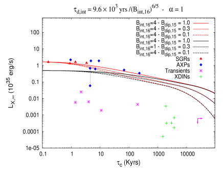
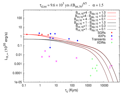
Figure 8: Maximum surface luminosity as a function of $\tau_{c}$ of a NS with an internal magnetic field decaying through the solenoidal mode of ambipolar diffusion, with $\tau_{\rm d}\approx 9.6\times 10^{3}B^{-6/5}_{\rm int,16}~{}{\rm yrs}$. The magenta arrows indicate the current upper limits on the spindown age and $L_{\rm X}$ of SGR 0418+5729. Two initial values for the internal field are chosen, $B_{\rm int,i}=4\times 10^{16}$ G corresponds to red curves and $10^{16}$ G corresponds to black curves. For each value of the internal field, three values of the initial dipole, $B_{\rm dip,i}=10^{15},3\times 10^{14}$ and $10^{14}$ G were chosen, corresponding to the continuous, dashed and dot-dashed lines, respectively. Left Panel: The dipole field decays according to the $\alpha=1$ scaling, $\tau_{\rm d}=10^{3}~{}{\rm yrs}~{}B^{-1}_{\rm dip,15}$; Right Panel : The dipole field decays according to the $\alpha=1.5$ scaling, $\tau_{\rm d}=10^{3}~{}{\rm yrs}~{}B^{-1.5}_{\rm dip,15}$.

We stress that, in this regime, the former scaling $L_{\rm B,int}\propto B^{16/5}_{\rm int}$ does not hold anymore. We obtained $\alpha_{\rm int}=2/19$ which implies $L_{\rm B,int}\propto B^{40/9}_{\rm int}$, matching the evolution of $L_{\rm X}$ as it must, given the equilibrium condition we imposed in the photon-cooling phase.

In Fig. 8 we show $L_{\rm X,\infty}$ vs. $\tau_{\rm c}$ curves for two different values of the initial internal field and three different values of the initial dipole. Two different choices for the decay index, $\alpha=1$ or 1.5, are shown in the left and right panel of that figure, respectively. Note that curves for different values of $B_{\rm int,i}$ and the same value of $B_{\rm dip,i}$ become coincident, at late times. This happens because the surface luminosity tracks the instantaneous value of $B_{\rm int}$ and all models reach the same value of the internal field, at late times. On the other hand, curves with different $B_{\rm dip,i}$ and the same $B_{\rm int,i}$ maintain memory of the initial conditions although dipole fields also reach to the same value at late times. This happens because the relation between $\tau_{\rm c}$ and $t$ depends explictly on the initial dipole (cfr. Eq. 14). At a given $\tau_{\rm c}$, objects that had a different $B_{\rm dip,i}$ are not co-eval. Those who had a weaker initial dipole are older, have a weaker $B_{\rm int}$ and, thus, have a lower luminosity too.

The relatively flat evolution of $L_{\rm X}$ for sources with $\tau_{\rm c}<10^{4}$ yrs can be explained quite naturally, in this scenario. Larger initial fields produce larger luminosities (Eq. 30) but, at the same time, they have shorter decay times ($\tau_{\rm d,i}\propto B^{-6/5}_{\rm int,i}$). Hence, $L_{\rm X}$ is larger and bends earlier downwards for increasingly strong initial fields, with the result that a flat, narrow strip of sources is produced. Its spread in $L_{\rm X}$ is smaller than the spread in $B_{\rm int,i}$ and its maximum extension in $\tau_{\rm c}$ roughly corresponds to the decay time, $\tau_{\rm d,i}$ of the minimum field. We estimate $B^{{\rm(min)}}_{\rm int,i}\gtrsim 10^{16}$ G.

Two further properties of the above plots are worth noticing. First, the model with a faster decay of the dipole, $\alpha=1$, matches well the luminosities of persistent sources up to $\tau_{\rm c}\gtrsim 10^{5}$ yrs, but largely fails to account for the position of SGR 0418+5729. A direct link between the latter object and the persistent sources would then be impossible. Although the possibility that SGR 0418+5729 is linked to the transient sources is an interesting alternative, it has a serious drawback, if $\alpha=1$. A population of older ($\tau_{\rm c}\geq 10^{6}$ yrs), relatively bright magnetars would be expected, which is clearly not seen. All known sources at that $\tau_{\rm c}$ (or beyond) are much dimmer and, accordingly, this possibility seems ruled out.

The model with $\alpha=1.5$, on the other hand, provides a viable option to intepret SGR 0418+5729 as an older relative ($t_{\rm age}\sim 10^{6}$ yrs) of the persistent sources whose dipole, as well as internal, fields have strongly decayed. In particular, the two lower curves in the right panel of Fig. 8 give an internal field $B^{\rm{(0418)}}_{\rm int,14}\approx 1.6(1.1)$, a dipole field $B^{\rm{(0418)}}_{\rm dip,12}\approx 6(4)$ and an X-ray luminosity $L^{\rm{(0418)}}_{\rm X,30}\approx 30(0.4)$, respectively, from top to bottom. The predicted range of quiescent luminosities is quite wide, as opposed to the relatively narrow range for both $B_{\rm int}$ and $B_{\rm dip}$. This reflects the fact that SGR 0418+5729 is already in the photon-cooling dominated regime, where a steep drop in $L_{\rm X}$ occurs. A careful assessment of its actual quiescent emission would thus in principle put additonal constraints on the pysical parameters of this object.

7.2 Hall decay of the field in the inner crust

The calculation of the previous section rules out small values of $\alpha$ and points to $1.5\lesssim\alpha\lesssim 1.8$ as a viable option. Transition to core superfluidity ($T_{\rm c}<5\times 10^{8}$ K, Page et al. 2011) is expected to occur at an age $\gtrsim{\rm a~{}few}\times 10^{4}$ yrs, if $B_{\rm int,i}>10^{16}$ G, which for the viable values of $\alpha$ corresponds to $\tau_{\rm c}\sim 10^{5}$ yrs. As stated before, we currently don’t have a clear understanding of what will happen at this transition. The most conservative option is assuming that evolution of the core field will suddenly freez, its influence on the NS temperature soon becoming negligible.

Even in this case, however, an internal field that threaded the NS crust would still be actively decaying, due to the Hall term in the indcution equation. We consider here this “minimal heating scenario” for magnetars, focusing on the effect of field decay in the NS crust.

The timescale of Hall-driven decay of the magnetic field in NS crusts has a dependence on the actual field geometry, as was shown by Cumming et al. (2004). The field component that we are considering could either be a twisted (toroidal) field threading both core and crust (case $I$) or an azimuthal/multipolar field anchored only in the NS crust (case $II$). We consider the two cases separately.

7.2.1 Case $I$ Hall decay

If the decaying crustal field were threading both the NS core and crust, its decay timescale would be sensitive to the global structure and is expected to be longer than Eq. 25 by a factor $\sim R_{*}/h$, where $h$ is crust thickness Cumming et al. (2004). A more accurate expression was provided by Arras et al. (2004),

$$\tau^{(I)}_{\rm H}=\frac{2.4\times 10^{4}~{}\rho^{5/3}_{14}}{B_{16}}~{}{\rm yrs}~{}~{},$$ (34)

who also integrated the field induction equation through the crustal volume adopting this formula and a realistic density profile, to estimate the associated power output. The resulting expression

$$L^{(I)}_{\rm B,int}\approx 2\times 10^{36}B^{3}_{16}R_{*,6}~{}~{}{\rm erg\ s}^{-1}~{}~{},$$ (35)

exceeds the observed X-ray emission of younger sources if $B_{\rm int,i}\gtrsim 5\times 10^{15}\;$G, which accordingly represents a strict lower limit to the required crustal field. We evaluate the radiative efficiency of this model by considering, in a crude way, the impact of neutrino emitting processes within the NS crust. Neutrino bremsstrahlung and plasmon decay, in particular, become quickly very efficient in carrying away heat as the temperature rises, effectively limiting the maximum temperature that can be reached at the surface (cfr. TD96). An approximate, analytical expression for the implied maximum surface temperature, $T^{({\rm max})}_{\rm s}$, which also includes the effects of the magnetic field, was recently provided by (Pons et al., 2009)

$$T^{({\rm max})}_{\rm s}\simeq\frac{3.6\times 10^{6}~{}{\rm K}}{1+0.002~{}{\rm LogB_{12}}}\Rightarrow L^{({\rm max})}_{X,\infty}\approx 9\times 10^{34}R^{2}_{*,6}~{}{\rm ergs}^{-1}$$ (36)

where we neglect the very weak dependence on magnetic field in the last step. The effect on $T^{({\rm max})}_{\rm s}$ would be much more pronounced if the field were predominantly tangential to the surface, thus strongly inhibiting heat conduction in the radial direction (Yakovlev et al. 2007; Page et al. 2007; Pons & Geppert 2009). However, the X-ray emission in the sample of persistent sources is very close to the limit of Eq. 36 and much higher than the limit derived for a strong tangential field. The effects of such a component do not appear to be relevant, at least for these sources, as was already pointed out by Kaminker et al. (2009). On the other hand, the effects of a strong tangential field would be qualitatively consistent with the weak quiescent emission of transient sources. A proper account of this issue is beyond our scope here and is postponed to future work.

With the above formulae we can build approximate luminosity curves. As long as $L_{\rm B,int}$ calculated through Eq. 35 is larger than $L^{({\rm max})}_{\rm s}$ (Eq. 36), our curves are limited by the latter value. Once $L_{\rm B,int}$ becomes comparable to $L^{({\rm max})}_{\rm X}$ the radiative efficiency is close to one and our curves track the evolution of $L_{\rm B,int}$ from here on. The latter thus represents the bolometric luminosity of sources at later times. As in the previous section, we include the effect of gravitational redshift on the resulting $L_{\rm X}$. Note that the Hall timescale is independent of temperature, so the evolution of $L_{\rm B,int}$ extrapolates from the previous, $\nu$-limited regime, into the photon-cooling regime.

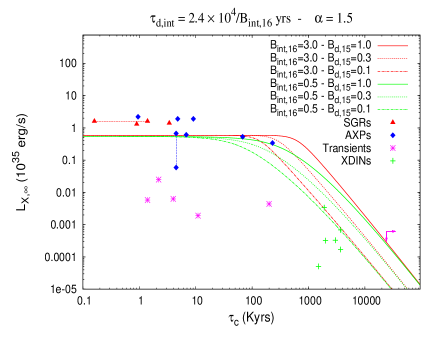
Figure 9: Curves show the evolution of the NS surface luminosity, as a function of $\tau_{\rm c}$, for Hall-driven decay of a field threading core and crust. The flat part of the curves corresponds to the maximum surface luminosity of Eq. 36 and lasts as long as $L_{\rm B,int}$ is larger than this limit. Once it drops below that, curves switch to $L_{\rm B,int}$ and, thus, represent the maximum available power from field decay (i.e. an upper limit to $L_{\rm X,\infty}$ in the (2-10) keV range). Points mark the measured luminosities in the $(2-10)$ keV range of magnetar candidates. The magenta arrows indicate the current upper limits on the spindown age and $L_{\rm X}$ of SGR 0418+5729. Different symbols are explained in the figure. Left Panel: the dipole field decays according to the case $\alpha=1$ of sec. 5, with the scaling $\tau_{\rm d}=10^{3}B^{-1}_{15}$ yrs. Two values for the initial internal field are chosen, $3\times 10^{16}$ G and $5\times 10^{15}$ G. For each value of $B_{\rm int,i}$, two curves are shown, corresponding to two different choices for the initial dipole field, $10^{15}$ G (upper curves) and $10^{14}$ G (lower curves). Right Panel: same as left panel, but the dipole field is assumed to follow the $\alpha=1.5$ case of sec. 5. For each value of the internal field, three values of $B_{\rm dip,i}=10^{15},3\times 10^{14}{\rm~{}and}~{}10^{14}$ G are chosen.

We calculated curves in the $L_{\rm X,\infty}$ vs. $\tau_{\rm c}$ plane in this way choosing two different values of the initial internal field, $B_{\rm int,i}$. For each value of $B_{\rm int,i}$, two values of the initial dipole, $B_{\rm dip,i}$, were chosen, giving four curves in total for each value of the decay index $\alpha$. Two different values of $\alpha$ were chosen and results for either choice are shown in the two panels of Fig. 9.

Our main conclusions are summarized as follows:

• the NS surface emission saturates at a level close to, but lower than, the observed luminosity of young AXPs/SGRs ($\tau_{\rm c}\lesssim 10^{4}$ yrs). Given the uncertainties and approximations implicit in the derivation of the limit in Eq. 36, the mismatch should not be regarded as a major issue. Further, as already noted, the gradual relaxation of a magnetospheric twist could provide an additional channel for release of the energy of the internal field directly at the NS surface. It is interesting to note that, despite not being limited by crustal neutrino processes in this case, a luminosity enhancement by just a factor of 2-3, at most, is all that is required to match the data, thus roughly confirming the overall energy budget estimated in our approximate calculations. A similar argument does not apply to the decaying parts of the curves, though, since those represent the evolution of $L_{\rm B,int}$, a limit that cannot be exceeded.

• internal fields $\gtrsim 10^{16}$ G are required also in this scenario. The minimal value $B_{\rm int,i}\gtrsim 5\times 10^{15}$ G provides a total magnetic power, $L^{(I)}_{\rm B,int}$, marginally consistent with $L_{\rm X,\infty}\approx 2\times 10^{35}{\rm reg\;s}^{-1}$ of the youngest sources. Properly accounting for the powerful bursting activity of young sources and for realistic values of the radiative efficiency, would certainly imply a significantly larger minimal field. A neat example of this is provided by the 27 December 2004 Giant Flare fron SGR 1806-20, which released $\sim 5\times 10^{46}\;$erg in high-energy photons. Even assuming that this was a unique event during the whole lifetime of the source, which we take to be $\tau_{\rm c}\simeq 1.4\times 10^{3}\;$yr, it would correspond to an average power output of $\sim 1.5\times 10^{36}$ erg s^-1, an order of magnitude larger than the quiescent emission.

• the internal field must also be able to provide its large power output for a sufficiently long time, as to match the duration of the apparent plateau in the $L_{\rm X,\infty}$ vs. $\tau_{\rm c}$ up to $\tau_{\rm c}\gtrsim 10^{4}$ yrs. This is comparable to the decay time of initial internal fields $\sim 10^{16}$ G.

  For a given value of $B_{\rm int,i}$, a strong initial dipole and/or a small $\alpha$ push the end of the plateau to larger $\tau_{\rm c}$, as discussed in sec. 7.1. This is why the $\alpha=1$ model fails by overpredicting luminosities at $\tau_{\rm c}\gtrsim 10^{5}$ yrs, unless dipole fields as low as $10^{14}$ G are assumed. Even for such a weak dipole, this model overpredicts the luminosity of SGR 0418+5729 and is thus ruled out. The $\alpha=1.5$ model seems, on the other hand, to well match the apparent bending at $\tau_{\rm c}\sim 10^{5}$ yrs, also remaining consistent with the position of SGR 0418+5729 (cfr. our estimate of its minimal power output in sec. 5).

Finally note that the value of $T^{\rm(max)}_{\rm s}$ used in this section (Eq. 36) would also apply in the case of core dissipation (sec. 7.1), where we ignored this effect and let the surface luminosity free to grow. Despite this, the surface luminosities calculated in sec. 7.1 are close to the maximum implied by Eq. 36 and very close, indeed, to the observed luminosities of magnetar candidates. In fact, also in that case the surface emission is limited by neutrino-emitting processes, which take place in the core rather than the crust.

7.2.2 Case $II$ Hall decay

Finally, we consider the Hall-driven decay of a purely crustal field. In this case, the field would be completely insensitive to conditions in the core and its decay time is correctly given by Eq. 25. In a way completely analogous to Eq. 35, it is possible to define the total power output in the crust for this case as

$$L^{(II)}_{\rm B,int}\approx 2.7\times 10^{37}B^{3}_{16}R_{*,6}~{}~{}{\rm ergs}^{-1}~{}~{}.$$ (37)

Fig. 10 depicts the results the same calculation of the previous section, adopting the decay timescale Eq. 25 and the corresponding magnetic luminosity, Eq. 37.

One conclusion can be drawn also in this case, which is in common to all other cases examined: an internal field of $\gtrsim 10^{16}$ G is required to explain the observed luminosities of active magnetars, in particular middle-aged ones ($\tau_{\rm c}\gtrsim 10^{5}$ yrs). Indeed, although the luminosity of the youngest sources is orders of magnitude less than the available $L_{\rm B,int}$ at that age, luminosities in excess of $10^{34}$ erg s^-1 are measured in middle-ages sources. This turns out to be a crucial property, since only fields larger than $10^{16}$ G have a sufficiently large energy reservoir to account for it.

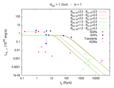
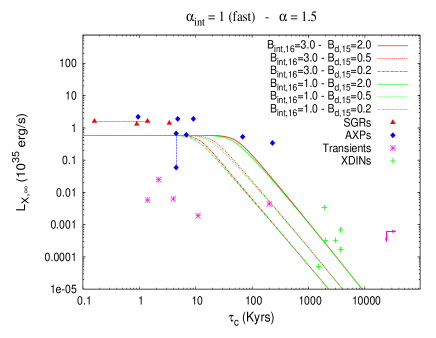
Figure 10: Curves show the evolution of the NS luminosity as a function of $\tau_{\rm c}$, for Hall-driven decay of a purely crustal field. The flat part of the curves corresponds to the maximum surface luminosity of Eq. 36 and lasts as long as $L_{\rm B,int}$ is larger than this limit. Once it drops below that, curves switch to $L_{\rm B,int}$ and, thus, represent the maximum available power from field decay (i.e. an upper limit to $L_{\rm X,\infty}$ in the (2-10) keV range). Points mark the measured luminosities in the $(2-10)$ keV range of magnetar candidates. Different symbols are explained in the figure. The magenta arrows indicate the current upper limits to the spindown age and $L_{\rm X}$ of SGR 0418+5729. Left Panel: the dipole field decays according to the case $\alpha=1$ of sec. 5, with the scaling $\tau_{\rm d}=10^{3}B^{-1}_{15}$ yrs. Two values for the initial internal field are chosen, $3\times 10^{16}$ G and $10^{16}$ G. For each value of the internal field, three curves are shown, corresponding to three different values of the initial dipole field, $2\times 10^{15}$ G, $5\times 10^{14}$ G and $2\times 10^{14}$ G. Right Panel: same as left panel, but the dipole field is assumed to follow the $\alpha=1.5$ case of sec. 5 and different representative values of $B_{\rm dip,i}$ are chosen.

For $\alpha=1$, it seems impossible to account for the luminosity of the AXPs 1E2259+586, even assuming the highest value of $B_{\rm dip,i}$ that is consistent with the distribution of sources of Fig. 3 and 4. The AXP 4U 0142+60 is, on the other hand, just marginally consistent with this upper curve. Note, however, that both sources correspond to a lower initial dipole, for $\alpha=1$, as shown in Fig. 3. If they were both born with $B_{\rm dip,i}=2\times 10^{15}$, their spin periods would have to be $\lesssim 11$ s, as clearly seen in Fig. 4. For $B_{\rm dip,i}\leq 10^{15}$ G the mismatch of model curves with observations would be far too large. This discrepancy is thus very significant.

A wide range of quiescent luminosities is predicted for SGR 0418+5729, essentially depending on its initial dipole field. The latter is likely close to $B_{\rm dip,i}\approx 10^{15}$ G for $\alpha=1$, (see Fig. 3 and 4), for which a quiescent luminosity $\sim 2\times 10^{31}$ erg s^-1 would be expected. A direct measurement of its quiescent emission may therefore provide a conclusive answer about this scenario.

The case $\alpha=1$ would have to be considered at best marginal, given the above considerations, essentially for the same reasons as the case $\alpha=1$ in sec. 6. The additional general arguments we presented against this small $\alpha$ value make this scenario, in conclusion, very unlikely.

The case $\alpha=1.5$ falls short of the X-ray emission of several sources beyond $\tau_{\rm c}\gtrsim 10^{5}$ yr and is, therefore, completely ruled out.

Overall, unless a different scaling for $\tau_{\rm Hall}$ can be provided, or unless an additional mechanism for decay of purely crustal fields is proposed, this hypothesis appears inconsistent with the observational properties of the source sample considered. Accordingly, we are led to rule it out in its present form.

8 Summary and Conclusions

In this work we have studied the implications of dipole field decay on the dynamical evolution of a spinning, magnetized NS, assuming a power-law scaling for the field decay time, $\tau_{\rm d}\propto B^{-\alpha}_{\rm dip}$ and $\dot{B}_{\rm dip}\propto B^{1+\alpha}_{\rm dip}$. If the field decays sufficiently fast ($\alpha<2$) the spindown time $\tau_{\rm c}$ grows faster than the decay time, $\tau_{\rm d}$. Once $\tau_{\rm c}>\tau_{\rm d}$, the dipole continues to decay while the NS spin period hardly changes and an asymptotic value of the spin period, $P_{\infty}$, is reached. For a slow ($\alpha>2$) decay, the above condition is never met and the NS continues spinning down forever.

The distribution of magnetar candidates (SGRs, AXPs, transients) and XDINs in the $B_{\rm dip}$ vs. $\tau_{\rm c}$ ( or $B_{\rm dip}$ vs. $P$) plane provides a strong evidence for a fast ($\alpha<2$) dipole field decay. This conclusion is based on two striking properties. First, the absence of objects with large periods, well above 10 s, and in particular with large dipole fields $B_{\rm dip}$ and large spindown ages $\tau_{\rm c}$. We know that objects with large $B_{\rm dip}$ exist since we find them at small $\tau_{\rm c}$. Similarly we know that objects with large $\tau_{\rm c}$ also exist, but they are all found only with relatively small $B_{\rm dip}$. If $B_{\rm dip}$ did not decay then $\tau_{\rm c}=t$ and there would be no reason why there are no old (large $\tau_{\rm c}$) objects with large $B_{\rm dip}$. Note that such objects should be more numerous that younger ones and they should be at least as detectable as objects with a similar $\tau_{\rm c}$ and smaller $B_{\rm dip}$.

Decay of the dipole field offers the most natural interpretation of this fact, as it naturally produces bending evolutionary tracks in the $B_{\rm dip}$ vs. $\tau_{\rm c}$ plane or, equivalently, the $\dot{P}$ vs. $P$ and $B_{\rm dip}$ vs. $P$ planes (see Figs. 3, 4 and 5). In particular, if the decay law has $\alpha<2$, an asymptotic spin period is approached which corresponds to the scaling $B_{\rm dip,15}\approx P_{\infty,10}~{}\tau^{-1/2}_{\rm c,kyr}$. Sources that reach their asymptotic period move along a trajectory with a constant period, $P_{\infty}$, which, in turn, is related to the value of $\alpha$ and of the initial magnetic dipole, $B_{\rm dip,i}$ (see Eq. 11).

The second key feature is the fact that spin period periods of all (but one) sources with $\tau_{\rm c}\geq 10^{4}\;$yr are within a very narrow strip corresponding to $7\lesssim P_{\infty}\lesssim 12$ s. This supports the existence of an asymptotic period and hence of a single decay mechanism operating in all sources, with $\alpha<2$ and with a decay time $\tau_{\rm d}\approx 10^{3}~{}B^{-\alpha}_{15}$ yr (sec. 5). The narrowness of the distribution in $P_{\infty}$ implies that the decay index must be in the range $1\lesssim\alpha<2$.

Hall decay in the crust, corresponding to $\alpha=1$, provides a reasonable explanation for the observed $B_{\rm dip}\,$–$\,\tau_{\rm c}$ distribution. It implies that all SGRs, AXPs, transients and XDINs were drawn from a distribution of $B_{\rm dip,i}\in[0.2-2]\times 10^{15}$ G. A similarly good description of the data is provided by larger values of $\alpha$, for which we consider $\alpha=1.5$ as representative. These allow for a wider distributions of initial dipoles, making them favored in this respect. As $\alpha$ approaches 2, asymptotic periods $>12$ s would necessarily be expected and the current data disfavor $\alpha$-values too close to 2. Note that all viable models imply that there cannot be a population of sources whose dipole field at birth is significantly larger than $\simeq 2\times 10^{15}$ G. These would indeed reach asymptotic spin periods significantly longer than observed.

An important implication of the dipole field decay with $\alpha<2$ is that the sources are younger than what their spindown age implies ($t<\tau_{\rm c}$). The current value of $t/\tau_{\rm c}$ also depends on $B_{\rm dip,i}$. For magnetar candidates this ratio is significantly smaller than unity and their real ages can be a factor of $\sim$5–50 smaller than $\tau_{\rm c}$, depending on their initial field, age, and exact value of $\alpha$.

The ratio $t/\tau_{\rm c}$ decreases for decreasing values of $\alpha$, at a given $\tau_{\rm c}$ (see Fig. 1). For a fixed value of $\alpha$, $t/\tau_{\rm c}$ decreases as the object ages.

X-ray luminosities of XDINs, their clustering at $\tau_{\rm c}\sim{\rm a\ few}\times 10^{6}\;$yr and the distribution of their effective temperatures point to their ages being $t\gtrsim 10^{5}\;$yr. This further constrains possible values of $\alpha$. Specifically, $\alpha=1$ decay implies that these sources are younger, or even much younger, than this value. On the other hand, values of $\alpha\sim 1.5$ well match this age requirement for XDINs. Thus, the case $\alpha=1$ is basically ruled out and a more restrictive condition, $1.5\lesssim\alpha\lesssim 1.8$, appears to be the most consistent with the whole available data.

Although the decaying dipole field dissipates energy, it turns out that unlike the simplest expectations, this energy is insufficient to power the strong X-ray emission of SGRs/AXPs (and, possibly, other related classes). While exponential decay is rapid enough that $L_{\rm B,dip}$ would suffice for all sources, the current upper limit on the weak quiescent emission of SGR 0418+5729 ($\lesssim 6\times 10^{31}$ erg s^-1) already implies $\alpha\gtrsim 1$, as otherwise this source would be too young to be so dim.

For $\alpha=1$, the maximal available power, $L_{\rm B,dip}$, falls short of the observed X-ray emission of persistent AXPs at $\tau_{\rm c}\approx 10^{5}\;$yr and the current observed emission of SGR 0418+5729 is far larger than its $L_{\rm B,dip}$ for all values of $\alpha\geq 1$. Hence, $\alpha=1$ and energy provided just by magnetic dipole field decay should be considered at best marginally consistent with the observed distribution of sources in the $L_{\rm X}$ vs. $\tau_{\rm c}$ plane. However, as we have discussed above, $\alpha=1$ is ruled out by the requirements on the ages of XDINs, which altogether imply $1.5\lesssim\alpha\lesssim 1.8$. For such values of $\alpha$ (or even for $\alpha>1$) it is impossible to power the X-ray emission of SGRs/AXPs by the decay of the dipole field. If magnetic energy powers this emission, the available reservoir must be larger than that of the dipole and must decay on a somewhat longer timescale. The most natural conclusion is that this is provided by the magnetic field in the NS interior (sec. 6).

In order to identify at least the basic properties of the internal field, we considered its decay either in the liquid core, through the solenoidal mode of ambipolar diffusion, or the inner crust, through the Hall term. In the latter case, we treat separately fields threading the whole NS volume or fields confined to the crust alone. A general conclusion in all cases is that the observed large $L_{\rm X}$ values at up to $\tau_{\rm c}\sim 10^{5}$ yrs require a very large initial internal field, $B_{\rm int,i}\gtrsim 10^{16}$ G . Combined with the maximum value of $\simeq 2\times 10^{15}$ G for the initial dipole field this implies that, at formation, the internal magnetic field in magnetars contains at least 20-30 times more energy than the dipole, likely one order of magnitude more than that. This raises a question about the stability of the implied configurations, which is a currently open field. Although it is difficult, at this stage, to have a precise answer on global field stability, recent investigations (cfr. Bra09) have highlighted the key role of stable stratification of stellar interiors in providing stability to predominantly toroidal fields. As opposed to this, it was shown that a predominantly poloidal field would remain unstable, independent of the interior stratification. The maximum ratio of toroidal-to-poloidal field strength that can be stablized is estimated, conservatively, to be $\lesssim 10$, for a $\sim 10^{16}$ G toroidal field, roughly consistent with our results. Clearly, more work is needed to settle this important topic.

Fields threading the NS core have relatively long decay timescales ($\gtrsim 10^{4}$ yr for $B_{\rm int}=10^{16}$ G), whether their dissipation occurs primarily in the crust or the liquid core. This implies that it takes $\gtrsim 10^{4}\;$yr for $L_{\rm X}$ to decrease appreciably. On the other hand, observations show that this decrease occurs at $\tau_{\rm c}\lesssim 10^{5}$ yrs, approximately 10 times larger than the real age. This favors values of $\alpha>1$ and, in particular, our choice $\alpha=1.5$ meets easily this requirement (cfr. Fig. 1). If $\alpha\simeq 1$, on the other hand, $\tau_{\rm c}$ grows too fast with real time and when $L_{\rm X}$ eventually starts decreasing, $\tau_{\rm c}$ is already too large, in sharp contrast with observations.

If the internal field is confined to the NS crust, on the other hand, it decays on a $\sim 10^{3}\;$yr timescale and the situation is reversed. The case $\alpha=1.5$ largely fails because it implies that a given $\tau_{\rm c}$ is reached when the source is too old and its X-ray emission too weak. The case $\alpha=1$ is marginally consistent with $\tau_{\rm c}\sim 10^{5}$ yr-old sources, and only for an extreme choice of parameter values. Considering the strong independent arguments against such a low $\alpha$ value, we conclude that purely crustal fields cannot account for the distribution of SGRs/AXPs in the $L_{\rm X}$ vs $\tau_{\rm c}$ plane.

SGR 0418+5729 has the largest $\tau_{\rm c}$, weakest $B_{\rm dip}$ and $L_{\rm X}$ of our sample and thus provides crucial insight into the long-term evolution of magnetar candidates. It is thus of particular interest to summarize our main conclusions on its properties. For the reasons just mentioned, we restrict attention to the two scenarios where the internal field threads the whole NS volume and, thus, to dipole field decay with $\alpha\approx 1.5$. We find very similar conclusions in the two cases, whether the internal field decays in the crust or liquid core. This is not surprising, given the very similar values of $\alpha_{\rm int}$ and $\tau_{\rm d,int}$ in both models. From the decay of the dipole field with $\alpha=1.5$, this source was likely born with $B_{\rm dip,i}\sim(3-5)\times 10^{14}$ G, which implies its real age is $t_{\rm age}\approx(1-2)\times 10^{6}$ yrs, the youngest age corresponding to the larger initial field. With these assumption on the initial dipole, its current dipole field would be $\sim(4-7)\times 10^{12}$ G and the internal field $B_{\rm int}\sim(1.1-2)\times 10^{14}$ G, independent of its initial value (as long as it was $\gtrsim 10^{16}$G). The average luminosity due to the decay of the internal field is $L_{\rm B,int}\approx L_{\rm X}\sim(4-10)\times 10^{30}$ erg s^-1.

Note that the internal field is expected to be close to the lower limit for being able to produce crust breaking (and, thus, bursts, according to the current understanding of these events, cfr. TD96; Perna & Pons 2011). Also note that the expected luminosity can be checked by continued monitoring of this source and is, incidentally, similar to the estimated average output from outbursts (cfr. sec. 5).

9 Discussion & Evolutionary Sequence

In the light of our results, we can sketch a tentative evolutionary picture for the different classes of objects considered here. The most obvious link is between SGRs and AXPs, as already suggested by Kouveliotou et al. (1998).

These sources appear to form a continuous sequence, with persistent SGRs seen as the youngest, mostly magnetized and brightest sources. Persistent AXPs are found at comparable field strength and similar, although slightly older, ages. A couple of evolved AXPs are known (1E2259+586 and 4U 0142+61), whose dipole fields have decayed substantially and whose X-ray luminosity is somewhat weaker than in younger objects. The X-ray luminosity of SGRs/AXPs is inconsistent with the decay of the dipole field alone and needs to be powered by an additional, stronger field component. The latter must thread the whole NS volume and its strength likely exceeds $10^{16}$ G at birth. At young ages the internal field likely decays through a combination of ambipolar diffusion in the core and Hall decay in the crust. The released heat powers the strong thermal emission typical of these sources. Neutrino-emitting processes, whether in the liquid core or in the crust, limit the thermal luminosity of young magnetars to be $\lesssim 10^{35}$ erg s^-1 and provide a likely explanation for the observed plateau in the distribution of $L_{\rm X}$ up to $\tau_{\rm c}\gtrsim 10^{4}$ yrs.

Transient SGRs/AXPs are not related in an obvious way to persistent sources. Their dipole fields are systematically weaker and their spin periods also appear to be shorter, on average, suggesting that most of them have not yet reached the asymptotic spin period. The two oldest transients have significantly weaker dipole fields and somewhat slower spins (CXO J164710-455216 and SGR 0418+5729), thus supporting this basic picture.

The decay of $B_{\rm dip}$ appears consistent with having the same properties as in persistent sources. However, the X-ray luminosities of transients are much weaker and it is not possible, at present, to identify a decline at $\tau_{\rm c}\approx 100$ kyrs, as seen in persistent sources.

The weak quiescent emission of transients is very striking, being much lower even than the power provided by their decaying dipole field. The relatively bright, short-time bursts they emit in outburst and the ensuing large increase in X-ray luminosities, that make them temporarily similar to the persistent sources, supports, on the other hand, their connection to the latter group If this is indeed the case, then, it is possible that transients also host a decaying, strong internal field, despite the very low radiative efficiency of their quiescent state. We can only speculate, at this stage, that a strong azimuthal component of the crustal field provides a possible explanation for their X-ray deficiency. If the energy released by magnetic dissipation is confined to a sufficient depth in the NS interior, thermal insulation of the hot regions by such a field component could suppress the surface X-ray emission by a large factor (cfr. Potekhin & Yakovlev 2001, Kaminker et al. 2009). The difference with persistent sources would then be attributed to the existence of a much more ordered field component in transients, which globally suppresses the radiative efficiency $\epsilon_{\rm X}$. Only at outbursts does the internal field gain access to the more efficient channel of X-ray radiation, probably due to flaring of smaller-scale field structures temporarily creating a preferential path for heat conduction, or a localized dissipation region close to the NS surface. This is qualitatively consistent with the small (and shrinking) emitting areas and high (and decreasing) temperatures of the extra BB spectral components found in outburst emission from transients.

In this context, the dichotomy in behaviour between transient and persistent SGRs/AXPs which likely represent two distinctevolutionary sequences (see Fig. 11), could point to a different mechanism for generation of their strong fields at formation. One might speculate, based on the apparent properties of their magnetic fields, that SGR/AXPs appear to be born with somewhat higher initial dipole fields ($B_{\rm dip,i}\sim 10^{15}\;$G) compared to transients (which are narrowly clustered around $B_{\rm dip,i}\sim 2\times 10^{14}\;$G). SGR/AXPs also have a strong initial internal chaotic field ($B_{\rm int,i}\gtrsim 10^{16}\;$G) that varies significantly on length scales much smaller than the NS radius, which naturally accounts for their good heat conduction from the core to the surface and for the more frequent and more powerful bursting activity. Transients, on the other hand, likely have a strong and globally ordered tangential field, which efficiently suppresses heat conduction from the core to the surface and also results in much fewer and smaller bursts (that are likely powered by small scale field structures). Thus, one might speculate that SGR/AXPs might attain their fields at birth through the alpha-omega dynamo, if they were initially sufficiently rapidly rotating, while NSs in the transient branch might obtain their fields through a different (unclear as of yet) mechanism.

The $B_{\rm dip}\,$ vs. $\,P$ distribution of XDINs is also consistent with the same dipole field decay of other classes. We conclude that these sources represent $\sim(1-6)\times 10^{5}$ year-old NSs born with $B_{\rm dip,i}\sim(0.03-2)\times 10^{15}\;$G (for $\alpha=1.5$; see bottom left panel of Fig. 3). Their initial dipole fields have significantly decayed, making them apparently look older than they really are. Hence, their weak X-ray emission is likely dominated by their remnant heat, although a minor contribution from the decay of their dipole field cannot be ruled out, in general. As opposed to other classes, they show no evidence for an additional, stronger field component in their interior. As such, their most likely connection is with other high-field NSs not showing any peculiar magnetar-like activity. The brighter XDINs had initial dipole fields comparable to those of SGR/AXPs or transients, but they likely have a weaker internal field. The dimmest and fastest spinning of all XDINs, RX J0420, was born with the weakest dipole field, $B_{\rm dip,i}\sim 4\times 10^{13}\;$G (for $\alpha=1.5$). This is well below that of SGR/AXPs, or even of transients, and actually suggests a possible evolutionary link with either the high B-field radio pulsars or the Rotation-Powered X-ray Pulsars (RPPs), which would depend on the strength (and, possibly, the geometry) of both the initial dipole field and the initial internal field. This tentative optionis also sketched in Fig. 11, alongside the clearer evolutionary tracks of the SGR/AXP branch and the transient branch, that have been discussed above.

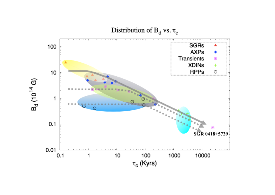
Figure 11: A schematic diagram of the evolutionary sequences we infer for different high magnetic field NS source classes in the $B_{\rm dip}\,$–$\,\tau_{\rm c}$ plane (which can be thought of as a rotated version of the $P\,$–$\,\dot{P}$ plane since $P\propto B_{\rm dip}\tau_{c}^{1/2}$ and $\dot{P}\propto B_{\rm dip}\tau_{\rm c}^{-1/2}$). Members of different classes are denoted by different symbols, while the classes as a whole are indicated by colored ellipses. We clearly identify two distinct evolutionary tracks – the SGR/AXP branch (solid arrow) and the transient branch (short-dashed arrow), which start with different initial dipole fields (and likely also different internal fields) but converge to similar values (at a given $\tau_{\rm c}$) after their fields decay significantly. The dimmest and fastest spinning XDIN (RX J0420) must have had a significantly smaller initial dipole field than either of these two branches, and thus must have followed a different evolutionary track, which might be related to rotation-powered X-ray pulsars (RPP) or high-field radio pulsars (this tentative track is indicated by the dotted arrow). Such a significantly lower initial dipole field results in a somewhat faster asymptotic spin period.

How does the “weak field magnetar” SGR 0418+5729 fit in the general picture? This object was likely born with a dipole field $\sim(3-5)\times 10^{14}$ G that has now decayed to $(4-7)\times 10^{12}$ G, and an internal field $\gtrsim 10^{16}$ G, which has now decayed to $\sim(1-2)\times 10^{14}\;$G. Despite its current appearance as a transient source, SGR 0418+5729 has most likely followed the track of persistent SGRs/AXPs in the $L_{\rm X}$ vs. $\tau_{\rm c}$ plane. The absence of more luminous sources at similar $\tau_{\rm c}$ implies that the emission of persistent sources must drop significantly in the range $\tau_{\rm c}\sim(10^{5}-10^{7}$) yrs. It is not clear whether the decrease in luminosity of the persistent sources passes through the upper tail of XDINs (like the lower curves in the right panel of Fig. 9 may suggest) or completely avoids them (like most curves in the right panels of Figs. 8 and 9). In the former case XDINs would be a less homogeneous class of sources, which included both passively cooling, high-field NSs and some old magnetars. This would also imply that SGR 0418+5729 follows the brightest XDINs along the same cooling sequence. Its quiescent luminosity should thus be orders of magnitude lower than that of the brightest XDINs. In the latter case, the XDINs are just passively cooling NSs, with no particular relation to persistent SGRs/AXPs, accidentally occupying a region in parameter space that is between persistent and transient magnetars.

Overall we have demonstrated that the dipole magnetic field of magnetars must decay on a time scale of $(10^{3}/B^{\alpha}_{\rm dip,15})$ years. The most likely decay law has $1.5\lesssim\alpha\lesssim 1.8$. At the same time we have shown that the power supplied by the decaying dipole field is not sufficient to power the X-ray luminosity of these objects. Unless there is an external energy reservoir, like a fallback disk (cfr. Trümper et al. 2010; Alpar et al. 2011), this energy can arise only from a stronger internal field whose decay is decoupled from the decay of the dipole. Detailed analyses of the X-ray emission depends on the structure of this internal field, its decay mode as well as cooling and heat transfer within the NS. Further observations of this exciting group of object could reveal some of the hidden secrets of the NS interiors as well as provide clues on magnetic field generation and amplification at their birth.

References

- Alpar et al. (2011) Alpar, M. A., Ertan, Ü., & Çalışkan, Ş., 2011, ApJL., 732, L4
- Arras et al. (2004) Arras P., Cumming A., Thompson C., 2004, ApJL., 608, L49
- Beloborodov (2009) Beloborodov A. M., 2009, ApJ., 703, 1044
- Beloborodov & Thompson (2007) Beloborodov A. M., Thompson C., 2007, ApJ., 657, 967
- Bernardini et al. (2009) Bernardini F., Israel G. L., Dall’Osso S., Stella L., Rea N., Zane S., Turolla R., Perna R., Falanga M., Campana S., Götz D., Mereghetti S., Tiengo A., 2009, Astron. & Astrophys., 498, 195
- Braithwaite (2009) Braithwaite, J., 2009, MNRAS, 397, 763
- Camilo et al. (2007) Camilo F., Ransom S. M., Halpern J. P., Reynolds J., 2007, ApJL., 666, L93
- Camilo et al. (2006) Camilo F., Ransom S. M., Halpern J. P., Reynolds J., Helfand D. J., Zimmerman N., Sarkissian J., 2006, Nature, 442, 892
- Cline et al. (1998) Cline T. L., Mazets E. P., Golenetskii S. V., 1998, IAU Circ., 7002, 1
- Colpi et al. (2000) Colpi M., Geppert U., Page D., 2000, ApJL., 529, L29
- Cumming et al. (2004) Cumming A., Arras P., Zweibel E., 2004, ApJ., 609, 999
- Dall’Osso et al. (2009) Dall’Osso S., Shore S. N., Stella L., 2009, MNRAS, 398, 1869
- Durant & van Kerkwijk (2006) Durant M., van Kerkwijk M. H., 2006, ApJ., 650, 1070
- Esposito et al. (2010) Esposito P., Israel G. L., Turolla R., Tiengo A., Götz D., de Luca A., Mignani R. P., Zane S., Rea N., Testa V., Caraveo P. A., Chaty S., Mattana F., Mereghetti S., Pellizzoni A., Romano P., 2010, MNRAS, 405, 1787
- Gaensler et al. (1999) Gaensler B. M., Gotthelf E. V., Vasisht G., 1999, ApJL., 526, L37
- Gaensler et al. (2005) Gaensler B. M., McClure-Griffiths N. M., Oey M. S., Haverkorn M., Dickey J. M., Green A. J., 2005, ApJL., 620, L95
- Gavriil et al. (2008) Gavriil F. P., Gonzalez M. E., Gotthelf E. V., Kaspi V. M., Livingstone M. A., Woods P. M., 2008, Science, 319, 1802
- Gavriil et al. (2002) Gavriil F. P., Kaspi V. M., Woods P. M., 2002, Nature, 419, 142
- Glampedakis et al. (2011) Glampedakis K., Jones D. I., Samuelsson L., 2011, MNRAS, 413, 2021
- Goldreich & Reisenegger (1992) Goldreich P., Reisenegger A., 1992, ApJ., 395, 250
- Heyl & Kulkarni (1998) Heyl J. S., Kulkarni S. R., 1998, ApJL., 506, L61
- Hollerbach & Rüdiger (2002) Hollerbach, R., Rüdiger, G. 2002, MNRAS, 337, 216
- Hurley et al. (1999) Hurley K., Cline T., Mazets E., Barthelmy S., Butterworth P., Marshall F., Palmer D., Aptekar R., Golenetskii S., Il’Inskii V., Frederiks D., McTiernan J., Gold R., Trombka J., 1999, Nature, 397, 41
- Ibrahim et al. (2004) Ibrahim A. I., Markwardt C. B., Swank J. H., Ransom S., Roberts M., Kaspi V., Woods P. M., Safi-Harb S., Balman S., Parke W. C., Kouveliotou C., Hurley K., Cline T., 2004, ApJL., 609, L21
- Jones (1988) Jones P. B., 1988, MNRAS, 233, 875
- Jones (2006) Jones P. B., 2006, MNRAS, 365, 339
- Kaminker et al. (2009) Kaminker A. D., Potekhin A. Y., Yakovlev D. G., Chabrier G., 2009, MNRAS, 395, 2257
- Kaplan (2008) Kaplan D. L., 2008, in Y.-F. Yuan, X.-D. Li, & D. Lai ed., Astrophysics of Compact Objects Vol. 968 of American Institute of Physics Conference Series, Nearby, Thermally Emitting Neutron Stars. pp 129–136
- Kaplan & van Kerkwijk (2011) Kaplan D. L., van Kerkwijk M. H., 2011, ApJL., 740, L30+
- Kaspi (2010) Kaspi V. M., 2010, Proceedings of the National Academy of Science, 107, 7147
- Kojima & Kisaka (2012) Kojima, Y., & Kisaka, S., 2012, arXiv:1201.1346
- Konenkov & Geppert (2001) Konenkov D., Geppert U., 2001, MNRAS, 325, 426
- Kouveliotou et al. (1998) Kouveliotou C., Dieters S., Strohmayer T., van Paradijs J., Fishman G. J., Meegan C. A., Hurley K., Kommers J., Smith I., Frail D., Murakami T., 1998, Nature, 393, 235
- Kuiper et al. (2006) Kuiper L., Hermsen W., den Hartog P. R., Collmar W., 2006, ApJ., 645, 556
- Kumar & Safi-Harb (2008) Kumar H. S., Safi-Harb S., 2008, ApJL., 678, L43
- Levin et al. (2010) Levin L., Bailes M., Bates S., Bhat N. D. R., Burgay M., Burke-Spolaor S., D’Amico N., Johnston S., Keith M., Kramer M., Milia S., Possenti A., Rea N., Stappers B., van Straten W., 2010, ApJL., 721, L33
- Mazets et al. (1979) Mazets E. P., Golentskii S. V., Ilinskii V. N., Aptekar R. L., Guryan I. A., 1979, Nature, 282, 587
- Mereghetti (2008) Mereghetti S., 2008, Astron. & Astroph. Review, 15, 225
- Mereghetti (2011) Mereghetti S., 2011, in D. F. Torres & N. Rea ed., High-Energy Emission from Pulsars and their Systems X-ray emission from isolated neutron stars. pp 345–+
- Mereghetti & Stella (1995) Mereghetti S., Stella L., 1995, ApJL., 442, L17
- Paczynski (1992) Paczynski B., 1992, Acta Astronomica, 42, 145
- Page et al. (2004) Page D., Lattimer J. M., Prakash M., Steiner A. W., 2004, Ap.J.Suppl., 155, 623
- Page, Geppert & Küker (2007) Page D., Geppert U., Küker M., 2007, Astroph. & Space Science, 308, 403
- Page et al. (2011) Page D., Prakash M., Lattimer J. M., Steiner A. W., 2011, Physical Review Letters, 106, 081101
- Palmer et al. (2005) Palmer D. M., Barthelmy S., Gehrels N., Kippen R. M., Cayton T., Kouveliotou C., Eichler D., Wijers R. A. M. J., Woods P. M., Granot J., Lyubarsky Y. E., Ramirez-Ruiz E., Barbier L., Chester M., Cummings J., Fenimore E. E., Finger M. H., Gaensler B. M., Hullinger D., Krimm H., Markwardt C. B., Nousek J. A., Parsons A., Patel S., Sakamoto T., Sato G., Suzuki M., Tueller J., 2005, Nature, 434, 1107
- Perna & Pons (2011) Perna R., Pons J. A., 2011, ApJL., 727, L51+
- (47) Pethick, C. J., & Sahrling, M., 1995, ApJL., 453, L29
- Pons & Geppert ( 2007) Pons J. A., Geppert U., 2007, Astron. & Astrophys., 470, 303
- Pons & Geppert (2010) Pons J. A., Geppert U., 2010, Astron. & Astrophys., 513, L12+
- Pons et al. (2009) Pons J. A., Miralles J. A., Geppert U., 2009, Astron. & Astrophys., 496, 207
- Potekhin & Yakovlev (2009) Potekhin A. Y., Yakovlev D. G., 2001, Astron. & Astrophys., 374, 213
- Rea & Esposito (2011) Rea N., Esposito P., 2011, in D. F. Torres & N. Rea ed., High-Energy Emission from Pulsars and their Systems Magnetar outbursts: an observational review. pp 247–+
- Rea et al. (2010) Rea N., Esposito P., Turolla R., Israel G. L., Zane S., Stella L., Mereghetti S., Tiengo A., Götz D., Göğüş E., Kouveliotou C., 2010, Science, 330, 944
- Rheinhardt & Geppert (2002) Rheinhardt M., Geppert U., 2002, Physical Review Letters, 88, 101103
- Shalybkov & Urpin (1997) Shalybkov, D. A., & Urpin, V. A., 1997, Astron. & Astrophys., 321, 685
- Spitkovsky (2006) Spitkovsky A., 2006, ApJL., 648, L51
- Terasawa et al. (2005) Terasawa T., Tanaka Y. T., Takei Y., Kawai N., Yoshida A., Nomoto K., Yoshikawa I., Saito Y., Kasaba Y., Takashima T., Mukai T., Noda H., Murakami T., Watanabe K., Muraki Y., Yokoyama T., Hoshino M., 2005, Nature, 434, 1110
- Thompson & Duncan (1995) Thompson C., Duncan R. C., 1995, MNRAS, 275, 255
- Thompson & Duncan (1996) Thompson C., Duncan R. C., 1996, ApJ., 473, 322
- Thompson & Duncan (2001) Thompson C., Duncan R. C., 2001, ApJ., 561, 980
- Thompson et al. (2002) Thompson C., Lyutikov M., Kulkarni S. R., 2002, ApJ., 574, 332
- Trümper et al. (2010) Trümper, J. E., Zezas, A., Ertan, Ü., & Kylafis, N. D., 2010, Astron. & Astrophys., 518, A46
- Turolla (2009) Turolla R., 2009, in W. Becker ed., Astrophysics and Space Science Library Vol. 357 of Astrophysics and Space Science Library, Isolated Neutron Stars: The Challenge of Simplicity. pp 141–+
- Turolla et al. (2011) Turolla R., Zane S., Pons J. A., Esposito P., Rea N., 2011, ArXiv e-prints
- Urpin, Chanmugam & Sang (1994) Urpin, V. A., Chanmugam, G., & Sang, Y., 1994, ApJ., 433, 780
- Urpin, Konenkov & Urpin ( 1997) Urpin, V., Konenkov, D., & Urpin, V., 1997, MNRAS, 292, 167
- Urpin & Konenkov ( 2008) Urpin, V., & Konenkov, D., 2008, Astron. & Astrophys., 483, 223
- Vainshtein et al. (2000) Vainshtein S. I., Chitre S. M., Olinto A. V., 2000, Phys. Rev. E, 61, 4422
- van der Horst et al. (2010) van der Horst A. J., Connaughton V., Kouveliotou C., Göğüş E., Kaneko Y., Wachter S., Briggs M. S., Granot J., Ramirez-Ruiz E., Woods P. M., Aptekar R. L., Barthelmy S. D., Cummings J. R., Finger M. H., Frederiks D. D., Gehrels N., Gelino C. R., Gelino D. M., Golenetskii S., Hurley K., Krimm H. A., Mazets E. P., McEnery J. E., Meegan C. A., Oleynik P. P., Palmer D. M., Pal’shin V. D., Pe’er A., Svinkin D., Ulanov M. V., van der Klis M., von Kienlin A., Watts A. L., Wilson-Hodge C. A., 2010, ApJL., 711, L1
- Woods & Thompson (2006) Woods P. M., Thompson C., 2006, Soft gamma repeaters and anomalous X-ray pulsars: magnetar candidates. pp 547–586
- Yakovlev & Pethick (2004) Yakovlev D. G., Pethick C. J., 2004, Ann. Rev. Astron. & Astrophys., 42, 169