Realization of metric spaces as inverse limits, and bilipschitz embedding in $L_{1}$

Abstract.

We give sufficient conditions for a metric space to bilipschitz embed in $L_{1}$. In particular, if $X$ is a length space and there is a Lipschitz map $u:X\to\mathbb{R}$ such that for every interval $I\subset\mathbb{R}$, the connected components of $u^{-1}(I)$ have diameter $\leq\operatorname{const}\cdot\operatorname{diam}(I)$, then $X$ admits a bilipschitz embedding in $L_{1}$. As a corollary, the Laakso examples [Laa00] bilipschitz embed in $L_{1}$, though they do not embed in any any Banach space with the Radon-Nikodym property (e.g. the space $\ell_{1}$ of summable sequences).

The spaces appearing the statement of the bilipschitz embedding theorem have an alternate characterization as inverse limits of systems of metric graphs satisfying certain additional conditions. This representation, which may be of independent interest, is the initial part of the proof of the bilipschitz embedding theorem. The rest of the proof uses the combinatorial structure of the inverse system of graphs and a diffusion construction, to produce the embedding in $L_{1}$.

1. Introduction

Overview

This paper is part of a series [CK06b, CK06a, CK10a, CK09, CK10b, CKN09, CKc] which examines the relations between differentiability properties and bilipschitz embeddability in Banach spaces. We give a new criterion for metric spaces to bilipschitz embed in $L_{1}$. This applies to several known families of spaces, illustrating the sharpness of earlier nonembedding theorems. In the first part of the proof, we characterize a certain class of metric spaces as inverse limits; this may be of independent interest.

Metric spaces sitting over $\mathbb{R}$

We begin with a special case of our main embedding theorem.

Theorem 1.1.

Let $X$ be a length space. Suppose $u:X\to\mathbb{R}$ is a Lipschitz map, and there is a $C\in(0,\infty)$ such that for every interval $I\subset\mathbb{R}$, each connected component of $u^{-1}(I)$ has diameter at most $C\cdot\operatorname{diam}(I)$. Then $X$ admits a bilipschitz embedding $f:X\to L_{1}(Z,\mu)$, for some measure space $(Z,\mu)$.

We illustrate Theorem 1.1 with two simple examples:

Example 1.2 (Lang-Plaut [LP01], cf. Laakso [Laa00]).

We construct a sequence of graphs $\{X_{i}\}_{i\geq 0}$ where $X_{i}$ has a path metric so that every edge has length $4^{-i}$. Let $X_{0}$ be the unit interval $[0,1]$. For $i>0$, inductively construct a $X_{i}$ from $X_{i-1}$ by replacing each edge of $X_{i-1}$ with a copy of the graph $\Gamma$ in Figure 1, rescaled by the factor $m^{-(i-1)}$. The graphs $X_{1}$, $X_{2}$, and $X_{3}$ are shown. The sequence $\{X_{i}\}$ naturally forms an inverse system,

$$X_{0}\stackrel{{\scriptstyle\pi_{0}}}{{\longleftarrow}}\cdots\stackrel{{\scriptstyle\pi_{i}}}{{\longleftarrow}}X_{i}\stackrel{{\scriptstyle\pi_{i+1}}}{{\longleftarrow}}\cdots\,,$$

where the projection map $\pi_{i-1}:X_{i}\to X_{i-1}$ collapses the copies of $\Gamma$ to intervals. The inverse limit $X_{\infty}$ has a metric $d_{\infty}$ given by

(1.3) $$d_{\infty}(x,x^{\prime})=\lim_{i\to\infty}\;d_{X_{i}}(\pi_{i}^{\infty}(x),\pi_{i}^{\infty}(x^{\prime}))\,,$$

where $\pi_{i}^{\infty}:X_{\infty}\to X_{i}$ denotes the canonical projection. (Note that the sequence of metric spaces $\{X_{i}\}_{i\geq 0}$ Gromov-Hausdorff converges to $(X_{\infty},d_{\infty})$.) It is not hard to verify that $\pi_{0}^{\infty}:(X_{\infty},d_{\infty})\to[0,1]$ satisfies the hypotheses of Theorem 1.1.

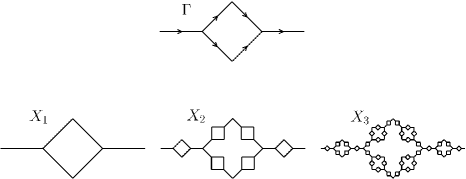
Figure 1.

Example 1.4.

Construct an inverse system

$$X_{0}\stackrel{{\scriptstyle\pi_{0}}}{{\longleftarrow}}\cdots\stackrel{{\scriptstyle\pi_{i}}}{{\longleftarrow}}X_{i}\stackrel{{\scriptstyle\pi_{i+1}}}{{\longleftarrow}}\cdots$$

inductively as follows. Let $X_{0}=[0,1]$. For $i>0$, inductively define $X_{i-1}^{\prime}$ to be the result of trisecting all edges in $X_{i-1}$, and let $N\subset X_{i-1}^{\prime}$ be new vertices added in trisection. Now form $X_{i}$ by taking two copies of $X_{i-1}^{\prime}$ and gluing them together along $N$. More formally,

$$X_{i}=(X_{i-1}^{\prime}\times\{0,1\})/\sim\,,$$

where $(v,0)\sim(v,1)$ for all $v\in N$. The map $\pi_{i-1}:X_{i}\to X_{i-1}$ is induced by the collapsing map $X_{i-1}^{\prime}\times\{0,1\}\ni(x,j)\mapsto x\in X_{i-1}$. Metrizing the inverse limit $X_{\infty}$ as in Example 1.2, the canonical projection $X_{\infty}\to X_{0}\simeq[0,1]\to\mathbb{R}$ satisfies the assumptions of Theorem 1.1.

The inverse limit $X_{\infty}$ in Example 1.4 is actually bilipschitz homeomorphic to one of the Ahlfors regular Laakso spaces from [Laa00], see Section 10. Thus Theorem 1.1 implies that this Laakso space bilipschitz embeds in $L_{1}$ (this special case was announced in [CK06b]). Laakso showed that $X_{\infty}$ carries a doubling measure which satisfies a Poincaré inequality, and using this, the nonembedding result of [CK09] implies that $X_{\infty}$ does not bilipschitz embed in any Banach space which satisfies the Radon-Nikodym property. Therefore we have:

Corollary 1.5.

There is a compact Ahlfors regular (in particular doubling) metric measure space satisfying a Poincaré inequality, which bilipschitz embeds in $L_{1}$, but not in any Banach space with the Radon-Nikodym property (such as $\ell_{1}$).

To our knowledge, this is the first example of a doubling space which bilipschitz embeds in $L_{1}$ but not in $\ell_{1}$.

We can extend Theorem 1.1 by dropping the length space condition, and replacing connected components with a metrically based variant.

Definition 1.6.

Let $Z$ be a metric space and $\delta\in(0,\infty)$. A $\delta$-path (or $\delta$-chain) in $Z$ is a finite sequence of points $z_{0},\ldots,z_{k}\subset Z$ such that $d(z_{i-1},z_{i})\leq\delta$ for all $i\in\{1,\ldots,k\}$. The property of belonging to a $\delta$-path defines an equivalence relation on $Z$, whose cosets are the $\delta$-components of $Z$.

Our main embedding result is:

Theorem 1.7.

Let $X$ be a metric space. Suppose there is a $1$-Lipschitz map $u:X\to\mathbb{R}$ and a constant $C\in(0,\infty)$ such that for every interval $I\subset\mathbb{R}$, the $\operatorname{diam}(I)$-components of $u^{-1}(I)$ have diameter at most $C\cdot\operatorname{diam}(I)$. Then $X$ admits a bilipschitz embedding $f:X\to L_{1}$.

Inverse systems of directed metric graphs, and multi-scale factorization

Our approach to proving Theorem 1.7 is to first show that any map $u:X\to\mathbb{R}$ satisfying the hypothesis of theorem can be factored into an infinite sequence of maps, i.e. it gives rise to a certain kind of inverse system where $X$ reappears (up to bilipschitz equivalence) as the inverse limit. Strictly speaking this result has nothing to do with embedding, and can be viewed as a kind of multi-scale version of monotone-light factorization ([Eil34, Why34]) in the metric space category.

We work with a special class of inverse systems of graphs:

Definition 1.8 (Admissible inverse systems).

An inverse system indexed by the integers

$$\cdots\stackrel{{\scriptstyle\pi_{-i-1}}}{{\longleftarrow}}X_{-i}\stackrel{{\scriptstyle\pi_{-i}}}{{\longleftarrow}}\cdots\stackrel{{\scriptstyle\pi_{-1}}}{{\longleftarrow}}X_{0}\stackrel{{\scriptstyle\pi_{0}}}{{\longleftarrow}}\cdots\stackrel{{\scriptstyle\pi_{i}}}{{\longleftarrow}}X_{i}\stackrel{{\scriptstyle\pi_{i+1}}}{{\longleftarrow}}\cdots\,,$$

is admissible if for some integer $m\geq 2$ the following conditions hold:

1. $X_{i}$ is a nonempty directed graph for every $i\in\mathbb{Z}$.

2. For every $i\in\mathbb{Z}$, if $X_{i}^{\prime}$ denotes the directed graph obtained by subdividing each edge of $X_{i}$ into $m$ edges, then $\pi_{i}$ induces a map $\pi_{i}:X_{i+1}\to X_{i}^{\prime}$ which is simplicial, an isomorphism on every edge, and direction preserving.

3. For every $i,j\in\mathbb{Z}$, and every $x\in X_{i}$, $x^{\prime}\in X_{j}$, there is a $k\leq\min(i,j)$ such that $x$ and $x^{\prime}$ project to the same connected component of $X_{k}$.

Note that the $X_{i}$’s need not be connected or have finite valence, and they may contain isolated vertices.

We endow each $X_{i}$ with a (generalized) path metric $d_{i}:X_{i}\times X_{i}\to[0,\infty]$, where each edge is linearly isometric to the interval $[0,m^{-i}]\subset\mathbb{R}$. Since we do not require the $X_{i}$’s to be connected, we have $d_{i}(x,x^{\prime})=\infty$ when $x,x^{\prime}$ lie in different connected components of $X_{i}$. It follows from Definition 1.8 that the projection maps $\pi_{i}^{j}:(X_{j},d_{j})\to(X_{i},d_{i})$ are $1$-Lipschitz.

Examples 1.2 and 1.4 provide admissible inverse systems in a straightforward way: for $i<0$ one simply takes $X_{i}$ to be a copy of $\mathbb{R}$ with the standard subdivision into intervals of length $m^{-i}$, and the projection map $\pi_{i}:X_{i+1}\to X_{i}$ to be the identity map. Of course this modification does not affect the inverse limit.

Let $X_{\infty}$ be the inverse limit of the system $\{X_{i}\}$, and let $\pi_{i}^{j}:X_{j}\to X_{i}$, $\pi_{i}^{\infty}:X_{\infty}\to X_{i}$ denote the canonical projections for $i\leq j\in\mathbb{Z}$. We will often omit the superscripts and subscripts when there is no risk of confusion.

We now equip the inverse limit $X_{\infty}$ with a metric $\bar{d}_{\infty}$; unlike in the earlier examples, this is not defined as a limit of pseudo-metrics $d_{i}\circ\pi_{i}^{\infty}$.

Definition 1.9.

Let $\bar{d}_{\infty}:X_{\infty}\times X_{\infty}\to[0,\infty)$ be the supremal pseudo-distance on $X_{\infty}$ such that for every $i\in\mathbb{Z}$ and every vertex $v\in X_{i}$, if

$$\operatorname{St}(v,X_{i})=\cup\{e\mid e\;\text{is an edge of}\;X_{i},\;v\in e\}$$

is the closed star of $v$ in $X_{i}$, then the inverse image of $\operatorname{St}(v,X_{i})$ under the projection map $X_{\infty}\to X_{i}$ has diameter at most $2m^{-i}$. Henceforth, unless otherwise indicated, distances in $X_{\infty}$ will refer to $\bar{d}_{\infty}$.

In fact $\bar{d}_{\infty}$ is a metric, and for any distinct points $x,x^{\prime}\in X_{\infty}$, the distance $\bar{d}_{\infty}(x,x^{\prime})$ is comparable to $m^{-i}$, where $i$ is the maximal integer such that $\{\pi_{i}^{\infty}(x),\pi_{i}^{\infty}(x^{\prime})\}$ is contained in the star of some vertex $v\in X_{i}$; see Section 2. In Examples 1.2 and 1.4, the metric $\bar{d}_{\infty}$ is comparable to the metric $d_{\infty}$ defined using the path metrics in (1.3); see Section 3.

Admissible inverse systems give rise to spaces satisfying the hypotheses of Theorem 1.7:

Theorem 1.10.

Let $\{X_{i}\}$ be an admissible inverse system. Then there is a $1$-Lipschitz map $\phi:X_{\infty}\to\mathbb{R}$ which is canonical up to post-composition with a translation, which satisfies the assumptions of Theorem 1.7.

The converse is also true:

Theorem 1.11.

Let $X$ be a metric space. Suppose $u:X\to\mathbb{R}$ is a $1$-Lipschitz map, and there is a constant $C\in[1,\infty)$ such that for every interval $I\subset\mathbb{R}$, the inverse image $u^{-1}(I)\subset X$ has $\operatorname{diam}(I)$-components of diameter at most $C\cdot\operatorname{diam}(I)$. Then for any $m\geq 2$ there is an admissible inverse system $\{X_{i}\}$ and a compatible system of maps $f_{i}:X\to X_{i}$, such that:

• The induced map $f_{\infty}:X\to(X_{\infty},\bar{d}_{\infty})$ is $L^{\prime}=L^{\prime}(C,m)$-bilipschitz.

• $u=\phi\circ f_{\infty}$, where $\phi:X_{\infty}\longrightarrow\mathbb{R}$ is the $1$-Lipschitz map of Theorem 1.10.

Theorem 1.1 is a corollary of Theorem 1.11 : if $u:X\to\mathbb{R}$ is as in Theorem 1.1, then for any interval $[a,a+r]\subset\mathbb{R}$, an $r$-component of $f^{-1}([a,a+r])$ will be contained in a connected component of $f^{-1}([a-r,a+2r])$ (since $X$ is a length space), and therefore has diameter $\leq 3C\operatorname{diam}(I)$.

Remark 1.12.

Theorem 1.11 implies that Examples 1.2 and 1.4 can be represented up to bilipschitz homeomorphism as inverse limits of many different admissible inverse systems, since the integer $m$ may be chosen freely.

Remark 1.13.

Although it is not used elsewhere in the paper, in Section 11 we prove a result in the spirit of Theorem 1.11 for maps $u:X\to Y$, where $Y$ is a general metric space equipped with a sequence of coverings.

Analogy with light mappings in the topological category

We would like to point out that Theorems 1.10, 1.11 are analogous to certain results for topological spaces.

Recall that a continuous map $f:X\to Y$ is light (respectively discrete, monotone) if the point inverses $\{f^{-1}(y)\}_{y\in Y}$ are totally disconnected (respectively discrete, connected). If $X$ is a compact metrizable space, then $X$ has topological dimension $\leq n$ if and only if there is a light map $X\to\mathbb{R}^{n}$; one implication comes from the fact that closed light maps do not decrease topological dimension [Eng95, Theorem 1.12.4], and the other follows from a Baire category argument.

One may consider versions of light mappings in the Lipschitz category. One possibility is the notion appearing the Theorems 1.7 and 1.11:

Definition 1.14.

A Lipschitz map $f:X\to Y$ between metric spaces is Lipschitz light if there is a $C\in(0,\infty)$ such that for every bounded subset $W\subset Y$, the $\operatorname{diam}(W)$-components of $f^{-1}(W)$ have diameter $\leq C\cdot\operatorname{diam}(W)$.

The analog with the topological case then leads to:

Definition 1.15.

A metric space $X$ has Lipschitz dimension $\leq n$ iff there is a Lipschitz light map from $X\to\mathbb{R}^{n}$ where $\mathbb{R}^{n}$ has the usual metric.

With this definition, Theorems 1.7 and 1.11 become results about metric spaces of Lipschitz dimension $\leq 1$.

To carry the topological analogy further, we note that if $f:X\to Y$ is a light map between metric spaces and $X$ is compact, then [Dyc74, DU97], in a variation on monotone-light factorization, showed that there is an inverse system

$$Y\longleftarrow X_{1}\longleftarrow\ldots\longleftarrow X_{k}\longleftarrow\ldots$$

and a compatible family of mappings $\{g_{k}:X\to X_{k}\}$ such that:

• The projections $X_{k}\leftarrow X_{k+1}$ are discrete.

• $g_{k}$ gives a factorization of $f$:

  $$Y\longleftarrow X_{1}\longleftarrow\ldots\longleftarrow X_{k}\stackrel{{\scriptstyle g_{k}}}{{\longleftarrow}}X\,.$$

• The point inverses of $g_{k}$ have diameter $\leq\Delta_{k}$, where $\Delta_{k}\to 0$ as $k\to\infty$.

• $\{g_{k}\}$ induces a homeomorphism $g_{\infty}:X\to X_{\infty}$, where $X_{\infty}$ is the inverse limit $X_{\infty}$ of the system $\{X_{k}\}$.

Making allowances for the difference between the Lipschitz and topological categories, this compares well with Theorem 1.11.

Embeddability and nonembeddability of inverse limits in Banach spaces

Theorem 1.11 reduces the proof of Theorem 1.7 (and also Theorem 1.1) to:

Theorem 1.16.

Let $\{X_{i}\}_{i\in\mathbb{Z}}$ be an admissible inverse system, and $m$ be the parameter in Definition 1.8. There is a constant $L=L(m)\in(0,1)$ and a $1$-Lipschitz map $f:X_{\infty}\to L_{1}$ such that for all $x,y\in X_{\infty}$,

$$\|f(x)-f(y)\|_{L_{1}}\geq L^{-1}\,\bar{d}_{\infty}(x,y)\,.$$

In a forthcoming paper [CKa], we show that if one imposes additional conditions on an admissible inverse system $\{X_{i}\}$, the inverse limit $X_{\infty}$ will carry a doubling measure $\mu$ which satisfies a Poincaré inequality, such that for $\mu$ a.e. $x\in X_{\infty}$, the tangent space $T_{x}X_{\infty}$ (in the sense of [Che99]) is $1$-dimensional. The results apply to Examples 1.2 and 1.4. Moreover, in these two examples – and typically for the spaces studied in [CKa] – the Gromov-Hausdorff tangent cones at almost every point will not be bilipschitz homeomorphic to $\mathbb{R}$. The non-embedding result of [CK09] then implies that such spaces do not bilipschitz embed in Banach spaces which satisfy the Radon-Nikodym property. Combining this with Theorem 1.16, we therefore obtain a large class of examples of doubling spaces which embed in $L_{1}$, but not in any Banach space satisfying the Radon-Nikodym property, cf. Corollary 1.5.

Monotone geodesics

Suppose $\{X_{i}\}_{i\in\mathbb{Z}}$ is an admissible inverse system, and $\phi:X_{\infty}\to\mathbb{R}$ is as in Theorem 1.10. Then $\phi$ picks out a distinguished class of paths, namely the paths $\gamma:I\to X_{\infty}$ such that the composition $\phi\circ\gamma:I\to\mathbb{R}$ is a homeomorphism onto its image, i.e. $\phi\circ\gamma:I\to\mathbb{R}$ is a monotone. (This is equivalent to saying that the projection $\pi_{i}\circ\gamma:I\to X_{i}$ is either direction preserving or direction reversing, with respect to the direction on $X_{i}$.) It is not difficult to see that such a path $\gamma$ is a geodesic in $X_{\infty}$; see Section 2. We call the image of such a path $\gamma$ a monotone geodesic segment (respectively monotone ray, monotone geodesic ) if the image $\phi\circ\gamma(I)\subset\mathbb{R}$ is a segment (respectively is a ray, is all of $\mathbb{R}$). Monotone geodesics and related structures play an important role in the proof of Theorem 1.16. In fact, the proof of Theorem 1.16 produces an embedding $f:X_{\infty}\to L_{1}$ with the additional property that it maps monotone geodesic segments in $X_{\infty}$ isometrically to geodesic segments in $L_{1}$.

Now suppose $u:X\to\mathbb{R}$ is as in Theorem 1.11. As above, one obtains a distinguished family of paths $\gamma:I\to X$, those for which $u\circ\gamma:I\to\mathbb{R}$ is a homeomorphism onto its image. From the assumptions on $u$, it is easy to see that $u$ induces a bilipschitz homeomorphism from the image $\gamma(I)\subset X$ to the image $(u\circ\gamma)(I)\subset\mathbb{R}$, so $\gamma(I)$ is a bilipschitz embedded path. We call the images of such paths monotone, although they need not be geodesics. If $f_{\infty}:X\to X_{\infty}$ is a homeomorphism provided by Theorem 1.11, then $f_{\infty}$ maps monotone paths in $X$ to monotone segments/rays/geodesics in $X_{\infty}$ because $\phi\circ f_{\infty}=u$. Therefore, by combining Theorems 1.11 and 1.16, it follows that the embedding in Theorem 1.7 can be chosen to map monotone paths in $X$ to geodesics in $L_{1}$.

Discussion of the proof of Theorem 1.16

Before entering into the construction, we recall some observations from [CKb, CK10a, CK10b] which motivate the setup, and also indicate the delicacy of the embedding problem.

Let $\{X_{i}\}_{i\in\mathbb{Z}}$ be an admissible inverse system.

Suppose $f:X_{\infty}\to L_{1}$ is an $L$-bilipschitz embedding, and that $X_{\infty}$ satisfies a Poincaré inequality with respect to a doubling measure $\mu$ (e.g. Examples 1.2 and 1.4). Then there is a version of Kirchheim’s metric diffferentiation theorem [Kir94], which implies that for almost every $p\in X_{\infty}$, if one rescales the map $f$ and passes to a limit, one obtains an $L$-bilipschitz embedding $f_{\infty}:Z\to L_{1}$, where $Z$ is a Gromov-Hausdorff tangent space of $X_{\infty}$, such that $(f_{\infty})\mbox{\Large$|$\normalsize}_{\gamma}:\gamma\to L_{1}$ is a constant speed geodesic for every $\gamma\subset Z$ which arises as a limit of (a sequence of rescaled) monotone geodesics in $X_{\infty}$. When $X_{\infty}$ is self-similar, as in Examples 1.2 and 1.4, then $Z$ contains copies of $X_{\infty}$, and one concludes that $X_{\infty}$ itself has an $L$-bilipschitz embedding $X_{\infty}\to L_{1}$ which restricts to a constant speed geodesic embedding on each monotone geodesic $\gamma\subset X_{\infty}$. In view of this, and the fact that any bilipschitz embedding is constrained to have this behavior infinitesimally, our construction has been chosen so as to automatically satisfy the constraint, i.e. it generates maps which restrict to isometric embeddings on monotone geodesics.

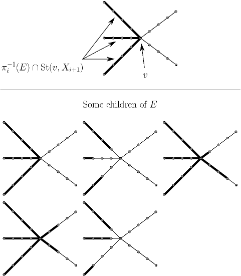
Figure 2.

By [Ass80, DL97, CK10a], producing a bilipschitz embedding $f:X_{\infty}\to L_{1}$ is equivalent to showing that distance function $\bar{d}_{\infty}$ is comparable to a cut metric $d_{\Sigma}$, i.e. a distance function $d_{\Sigma}$ on $X_{\infty}$ which is a superposition of elementary cut metrics. Informally speaking this means that

$$d_{\Sigma}=\int_{2^{X_{\infty}}}\;d_{E}\,d\Sigma(E)\,.$$

where $\Sigma$ is a cut measure on the subsets of $X_{\infty}$, and $d_{E}$ is the elementary cut (pseudo)metric associated with a subset $E\subset X_{\infty}$:

$$d_{E}(x_{1},x_{2})=|\chi_{E}(x_{1})-\chi_{E}(x_{2})|\,.$$

If $f:X_{\infty}\to L_{1}$ restricts to an isometric embedding $f\mbox{\Large$|$\normalsize}_{\gamma}:\gamma\to L_{1}$ for every monotone geodesic $\gamma\subset X_{\infty}$, then one finds (informally speaking) that the cut measure $\Sigma$ is supported on subsets $E\subset X_{\infty}$ with the property that for every monotone geodesic $\gamma\subset X_{\infty}$, the characteristic function $\chi_{E}$ restricts to a monotone function on $\gamma$, or equivalently, that the the intersections $E\cap\gamma$ and $(X_{\infty}\setminus E)\cap\gamma$ are both connected. We call such subsets monotone.

For simplicity we restrict the rest of our discussion to the case when $X_{0}\simeq\mathbb{R}$. The reader may find it helpful to keep Example 1.2 in mind (modified with $X_{i}\simeq\mathbb{R}$ for $i<0$ as indicated earlier).

Motived by the above observations, the approach taken in the paper is to obtain the cut metric $d_{\Sigma}$ as a limit of a sequence of cut metrics $\{d_{\Sigma_{i}^{\prime}}\}_{i\geq 0}$, where $\Sigma_{i}^{\prime}$ is a cut measure on $X_{i}$ supported on monotone subsets. For technical reasons, we choose $\Sigma_{i}^{\prime}$ so that every monotone subset $E$ in the support of $\Sigma_{i}^{\prime}$ is a subcomplex of $X_{i}^{\prime}$ (see Definition 1.8), and $E$ is precisely the set of points $x\in X_{i}$ such that there is a monotone geodesic $c:[0,1]\to X_{i}$ where $\pi_{0}^{i}\circ c$ is increasing, $c(0)=x$, and $c(1)$ lies in the boundary of $E$; thus one may think of $E$ as the set of points “lying to the left” of the boundary $\partial E$.

We construct the sequence $\{\Sigma_{i}^{\prime}\}$ inductively as follows. The cut measure $\Sigma_{0}^{\prime}$ is the atomic measure which assigns mass $\frac{1}{m}$ to each monotone subset of the form $(-\infty,v]$, where $v$ is vertex of $X_{0}^{\prime}\simeq\mathbb{R}$. Inductively we construct $\Sigma_{i+1}^{\prime}$ from $\Sigma_{i}^{\prime}$ by a diffusion process. For every monotone set $E\subset X_{i}$ in the support of $\Sigma_{i}^{\prime}$, we take the $\Sigma_{i}^{\prime}$-measure living on $E$, and redistribute it over a family of monotone sets $E^{\prime}\subset X_{i+1}$, called the children of $E$. The children of $E\subset X_{i}$ are monotone sets $E^{\prime}\subset X_{i+1}$ obtained from the inverse image $\pi_{i}^{-1}(E)$ by modifying the boundary locally: for each vertex $v$ of $X_{i+1}$ lying in the boundary of $\pi_{i}^{-1}(E)$, we move the boundary within the open star of $v$. An example of this local modification procedure is depicted in Figure 2, where $m=4$.

The remainder of the proof involves a series of estimates on the cut measures $\Sigma_{i}^{\prime}$ and cut metrics $d_{\Sigma_{i}^{\prime}}$, which are proved by induction on $i$ using the form of the diffusion process, see Section 7. One shows that the sequence of pseudo-metrics $\{\rho_{i}=d_{\Sigma_{i}^{\prime}}\circ\pi_{i}^{\infty}\}$ on $X_{\infty}$ converges geometrically to a distance function which will be the cut metric $d_{\Sigma}$ for a cut measure $\Sigma$ on $X_{\infty}$. To prove that $d_{\Sigma}$ is comparable to $d_{\infty}$, the idea is to show (by induction) that the cut metric $d_{\Sigma_{i}^{\prime}}$ resolves pairs of points $x_{1},x_{2}\in X_{i}$ whose separation is $>C\,m^{-i}$.

Organization of the paper

In Section 2 we collect notation and establish some basic properties of admissible inverse systems. Theorem 1.10 is proved in Section 2.3. Section 3 considers a special class of admissible inverse systems which come with natural metrics, e.g. Examples 1.2, 1.4. In Section 4 we prove Theorem 1.11. Sections 5–9 give the proof of Theorem 1.16. A special case of Theorem 1.16 is introduced in Section 5. In Section 6 we begin the proof of the special case by developing the structure of slices and associated slice measures, which are closely related to the monotone sets in the above discussion of the proof of Theorem 1.16. Section 7 obtains estimates on the slice measures which are needed for the embedding theorem. Section 8 completes the proof of Theorem 1.16 in the special case introduced in Section 5. Section 9 completes the proof in the general case. Section 10 shows that the space in Example 1.4 is bilipschitz homeomorphic to a Laakso space from [Laa00]. In Section 11 we consider a generalization of Theorem 1.11 to maps $u:X\to Y$, where $Y$ is a general metric space equipped with a sequence of coverings.

We refer the reader to the beginnings of the individual sections for more detailed descriptions of their contents.

2. Notation and preliminaries

In this section $\{X_{i}\}_{i\in\mathbb{Z}}$ will be an admissible inverse system, and $m$ will be the parameter appearing in Definition 1.8.

2.1. Subdivisions, stars, and trimmed stars

Let $Z$ be a graph. Let $Z^{(k)}$ denote the $k$-fold iterated subdivision of $Z$, where each iteration subdivides every edge into $m$ subedges, and let $Z^{\prime}=Z^{(1)}$.

If $v$ is a vertex of a graph ${\mathcal{G}}$, then $\operatorname{St}(v,{\mathcal{G}})$ and $\operatorname{St}^{o}(v,{\mathcal{G}})$ denote the closed and open stars of $v$, respectively.

Definition 2.1.

Let $Z$ be a graph, and $v\in Z$ be a vertex. The trimmed star of $v$ in $Z$ is the union of the edges of $Z^{\prime}$ which lie in the open star $\operatorname{St}^{o}(v,Z)$, or alternately, the union of the edge paths in $Z^{\prime}$ starting at $v$, with $(m-1)$ edges. We denote the trimmed star by $\operatorname{TSt}(v,Z)$. We will only use this when $Z=X_{i}$ or $Z=X_{i}^{\prime}$ below.

Note that if $v$ is a vertex of $X_{i}$, then $\operatorname{TSt}(v,X_{i})$ is also the closed ball $\overline{B(v,\frac{m-1}{m}\cdot m^{-i})}\subset X_{i}$ with respect to the path metric $d_{i}$.

2.2. Basic properties of admissible inverse systems and the distance function $\bar{d}_{\infty}$

Let $\{X_{i}\}_{i\in\mathbb{Z}}$ be an admissible inverse system with inverse limit $X_{\infty}$. For every $i$, we let $V_{i}$ be the vertex set of $X_{i}$, and $V_{i}^{\prime}$ be the vertex set of $X_{i}^{\prime}$. For all $j\geq i$, let $\pi_{i}^{j}:X_{j}\to X_{i}$ be the composition $\pi_{j-1}\circ\ldots\circ\pi_{i}$. Then $\pi_{i}^{j}:X_{j}\to X_{i}^{(j-i)}$ is simplicial and restricts to an isomorphism on each edge. It is also $1$-Lipschitz with respect to the respective path metrics $d_{j}$ and $d_{i}$.

Lemma 2.2.

For every $x,x^{\prime}\in X_{\infty}$ there exist $i\in\mathbb{Z}$, $v\in V_{i}$ such that $x,x^{\prime}\in(\pi_{i}^{\infty})^{-1}(\operatorname{St}(v,X_{i}))$.

Proof.

By (3) of Definition 1.8, there is a $j\in\mathbb{Z}$ such that $\pi_{j}(x),\pi_{j}(x^{\prime})$ are contained in the same connected component of $X_{j}$. If $\gamma\subset X_{j}$ is a path from $\pi_{j}(x)$ to $\pi_{j}(x^{\prime})$ with $d_{j}$-length $N$, then for all $i\leq j$, the projection $\pi_{i}^{j}(\gamma)$ is a path in $X_{i}^{(j-i)}$ with $d_{i}$-length $\leq N$. Therefore if $N<m^{-i}$ then $\pi_{i}^{j}(\gamma)$ will be contained in $\operatorname{St}(v,X_{i})$ for some $i\in V_{i}$. ∎

Suppose $\hat{d}$ is a pseudo-distance on $X_{\infty}$ with the property that

$$\operatorname{diam}_{\hat{d}}((\pi_{j}^{\infty})^{-1}(\operatorname{St}(v,X_{j}))\leq 2m^{-j}$$

for all $j\in\mathbb{Z}$, $v\in V_{j}$. Then for every $x,x^{\prime}\in X_{\infty}$, we have $\hat{d}(x,x^{\prime})\leq 2m^{-i}$, where $i\in\mathbb{Z}$ is as in Lemma 2.2. It follows that the supremum $\bar{d}_{\infty}$ of all such pseudo-distance functions takes finite values, i.e. is a well-defined pseudo-distance function.

Lemma 2.3 (Alternate definition of $\bar{d}_{\infty}$).

Suppose $x,x^{\prime}\in X_{\infty}$. Then $\bar{d}_{\infty}(x,x^{\prime})$ is the infimum of the sums $\sum_{k=1}^{n}\,2m^{-i_{k}}$, such that there exists a finite sequence

$$x=x_{0},\ldots,x_{n}=x^{\prime}\in X_{\infty}$$

where $\{\pi^{\infty}_{i_{k}}(x_{k-1}),\pi_{i_{k}}^{\infty}(x_{k})\}$ is contained in the closed star $\operatorname{St}(v,X_{i_{k}})$ for some vertex $v$ of $X_{i_{k}}$, for every $k\in\{1,\ldots,n\}$.

Proof.

Let $\hat{d}_{\infty}(x,x^{\prime})\in[0,\infty]$ be the infimum defined above. By Lemma 2.2 the infimum will be taken over a nonempty set of sequences, and so $\hat{d}_{\infty}(x,x^{\prime})\in[0,\infty)$. It follows that $\hat{d}_{\infty}$ is a well-defined pseudo-distance satisfying the condition that $\operatorname{diam}_{\hat{d}_{\infty}}((\pi_{i}^{\infty})^{-1}(\operatorname{St}(v,X_{i}))\leq 2m^{-i}$ for every $v\in V_{i}$, $i\in\mathbb{Z}$. Therefore $\hat{d}_{\infty}\leq\bar{d}_{\infty}$ from the definition of $\bar{d}_{\infty}$. On the other hand the definition of $\bar{d}_{\infty}$ and the triangle inequality imply $\bar{d}_{\infty}\leq\hat{d}_{\infty}$. ∎

Lemma 2.4.

Suppose $x,x^{\prime}\in X_{\infty}$.

1. If $\bar{d}_{\infty}(x,x^{\prime})\leq m^{-j}$ for some $j\in\mathbb{Z}$, then $\pi_{j}(x),\pi_{j}(x^{\prime})$ belong to $\operatorname{St}(v,X_{j})$ for some $v\in V_{j}$.

2. If $x\in X_{\infty}$ and $r\leq\frac{(m-2)}{m}m^{-j}$ for some $j\geq 0$, then $\pi_{j}(B(x,r))$ is contained in the trimmed star $\operatorname{TSt}(v,X_{j})$ for some $v\in V_{j}$.

Proof.

(1). Pick $\epsilon>0$. Since $\bar{d}_{\infty}(x,x^{\prime})\leq m^{-j}$, there is a sequence $x=y_{0},\ldots,y_{k}=x^{\prime}\in X_{\infty}$, where for $\ell\in\{1,\ldots,k\}$, the points $y_{\ell-1},y_{\ell}$ lie in $\pi_{i_{\ell}}^{-1}(\operatorname{St}(v_{\ell},X_{i_{\ell}}))$, $v_{\ell}\in V_{i_{\ell}}$, and

$$\sum_{\ell}2m^{-i_{\ell}}\leq m^{-j}+\epsilon\,.$$

Taking $\epsilon<m^{-j}$, we may assume that $i_{\ell}\geq j$ for all $\ell\in\{1,\ldots,k\}$. Since $\pi_{i_{\ell}}(y_{\ell-1}),\pi_{i_{\ell}}(y_{\ell})\in\operatorname{St}(v_{\ell},X_{i_{\ell}})$, there is a path from $\pi_{i_{\ell}}(y_{\ell-1})$ to $\pi_{i_{\ell}}(y_{\ell})$ in $X_{i_{\ell}}$ of $d_{i_{\ell}}$-length $\leq 2m^{-i_{\ell}}$. Since $\pi_{j}^{i_{\ell}}:(X_{i_{\ell}},d_{i_{\ell}})\to(X_{j},d_{j})$ is $1$-Lipschitz for all $j$, we get that there is an path from $\pi_{j}(x)$ to $\pi_{j}(x^{\prime})$ in $X_{j}$ with $d_{j}$-length at most

$$\sum_{\ell}2m^{-i_{\ell}}<m^{-j}+\epsilon\,.$$

As $\epsilon$ is arbitrary, $\pi_{j}(x)$ and $\pi_{j}(x^{\prime})$ lie in $\operatorname{St}(v,X_{j})$ for some $j\in V_{j}$.

(2). The proof is similar to (1). ∎

Corollary 2.5.

$\bar{d}_{\infty}$ is a distance function on $X_{\infty}$.

Proof.

Suppose $x,x^{\prime}\in X_{\infty}$, $\bar{d}_{\infty}(x,x^{\prime})=0$, and $i\in\mathbb{Z}$. By Lemma 2.4, for all $j\geq i$ the set $\{\pi_{j}^{\infty}(x),\pi_{j}^{\infty}(x^{\prime})\}$ is contained in the star of some vertex $v\in V_{j}$. Since $\pi_{i}^{j}:(X_{j},d_{j})\to(X_{i},d_{i})$ is $1$-Lipschitz, it follows that $\{\pi_{i}^{\infty}(x),\pi_{i}^{\infty}(x^{\prime})\}$ is contained in a set of $d_{i}$-diameter $\leq 2m^{-j}$. Since $j$ is arbitrary, this means that $\pi_{i}^{\infty}(x)=\pi_{i}^{\infty}(x^{\prime})$. ∎

The following is a sharper statement:

Lemma 2.6.

Suppose $x_{1},x_{2}\in X_{\infty}$ are distinct points. Let $j$ be the minimum of the indices $k\in\mathbb{Z}$ such that $\{\pi_{k}(x_{1}),\pi_{k}(x_{2})\}$ is not contained in the trimmed star $\operatorname{TSt}(v,X_{k})$ for any $v\in V_{k}$. Then

(2.7) $$\frac{(m-2)}{m}m^{-j}<\bar{d}_{\infty}(x_{1},x_{2})\leq 2m^{-(j-1)}\,.$$

Proof.

The first inequality follows immediately from Lemma 2.4. By the choice of $j$, there is a vertex $v\in V_{j-1}$ such that

$$\{\pi_{j-1}(x_{1}),\pi_{j-1}(x_{2})\}\subset\operatorname{TSt}(v,X_{j-1})\subset\operatorname{St}(v,X_{j-1})\,,$$

so $\bar{d}_{\infty}(x_{1},x_{2})\leq 2m^{-(j-1)}$ by Definition 1.9.

∎

2.3. A canonical map from the inverse limit to $\mathbb{R}$

The next theorem contains Theorem 1.10.

Theorem 2.8.

Suppose $\{X_{i}\}$ is an admissible inverse system.

1. There is a compatible system of direction preserving maps $\phi_{i}:X_{i}\to\mathbb{R}$, such that for every $i$, the restriction of $\phi_{i}$ to any edge $e\subset X_{i}$ is a linear map onto a segment of length $m^{-i}$. In particular, $\phi_{i}$ is $1$-Lipschitz with respect to $d_{i}$.

2. The system of maps $\{\phi_{i}:X_{i}\to\mathbb{R}\}$ is unique up to post-composition with translation.

3. If $\phi:(X_{\infty},\bar{d}_{\infty})\to\mathbb{R}$ is the map induced by $\{\phi_{i}\}$, then $\phi$ is $1$-Lipschitz, and for every interval $I\subset\mathbb{R}$, the $\operatorname{diam}(I)$-components of $\phi^{-1}(I)$ have diameter at most $8m\cdot\operatorname{diam}(I)$.

Proof.

(1). Let $X_{-\infty}$ denote the direct limit of the system $\{X_{i}\}$, i.e. $X_{-\infty}$ is the disjoint union $\sqcup_{i\in\mathbb{Z}}\;X_{i}$ modulo the equivalence relation that $X_{i}\ni x\sim x^{\prime}\in X_{j}$ if and only if there is a $k\leq\min(i,j)$ such that $\pi_{k}^{i}(x)=\pi_{k}^{j}(x^{\prime})$. For every $i\in\mathbb{Z}$ there is a canonical projection map $\pi_{-\infty}^{i}:X_{i}\to X_{-\infty}$.

If $k\in\mathbb{Z}$, then for all $i\leq k$ let $X_{i}^{(k-i)}$ denote the $(k-i)$-fold iterated subdivision of $X_{i}$, as in Section 2.1. Thus $\pi_{i}^{j}:X_{j}^{(k-j)}\to X_{i}^{(k-i)}$ is simplicial for all $i\leq j\leq k$, and restricts to a direction-preserving isomorphism on each edge of $X_{j}^{(k-j)}$. Therefore the direct limit $X_{-\infty}$ inherits a directed graph structure, which we denote $X_{-\infty}^{(k-\infty)}$, and for all $i\leq k$, the projection map $\pi_{-\infty}^{i}:X_{i}^{(k-i)}\to X_{-\infty}^{(k-\infty)}$ is simplicial, and a directed isomorphism on each edge of $X_{i}^{(k-i)}$. Condition (3) of the definition of admissible systems implies that $X_{-\infty}^{(k-\infty)}$ is connected.

Note also that for all $k\leq l$, the graph $X_{-\infty}^{(l-\infty)}$ is canonically isomorphic to $(X_{-\infty}^{(k-\infty)})^{(l-k)}$. In particular, if $v,v^{\prime}$ are distinct vertices of $X_{-\infty}^{(k-\infty)}$, then their combinatorial distance in $X_{-\infty}^{(l-\infty)}$ is at least $m^{l-k}$; morever every vertex of $X_{-\infty}^{(l-\infty)}$ which is not a vertex of $X_{-\infty}^{(k-\infty)}$ must have valence $2$, since it corresponds to an interior point of an edge of $X_{-\infty}^{(k-\infty)}$. It follows that $X_{-\infty}^{(k-\infty)}$ can contain at most one vertex $v$ which has valence $\neq 2$. Thus $X_{-\infty}^{(k-\infty)}$ is either isomorphic to $\mathbb{R}$ with the standard subdivision, or to the union of a single vertex $v$ with a (possibly empty) collection of standard rays, each of which is direction-preserving isomorphic to either $(-\infty,0]$ or $[0,\infty)$ with the standard subdivision. In either case, there is clearly a direction preserving simplicial map $X_{-\infty}^{(k-\infty)}\to\mathbb{R}$ which is an isomorphism on each edge of $X_{-\infty}^{(k-\infty)}$. Precomposing this with the projection maps $X_{\infty}\to X_{k}\to X_{-\infty}$ gives the desired maps $\phi_{i}$.

(2). Any such system $\{\phi_{i}:X_{i}\to\mathbb{R}\}$ induces a map $\phi_{-\infty}:X_{-\infty}\to\mathbb{R}$, which for all $k\in\mathbb{Z}$ restricts to a direction preserving isomorphism on every edge of $X_{-\infty}^{(k-\infty)}$. From the description of $X_{-\infty}^{(k-\infty)}$, the map $\phi_{-\infty}$ is unique up to post-composition with a translation.

(3). If $x,x^{\prime}\in X_{\infty}$ and $\{\pi_{i}(x),\pi_{i}(x^{\prime})\}\subset\operatorname{St}(v,X_{i})$ for some $i\in\mathbb{Z}$, $v\in V_{i}$, then by (1) $\{\phi(x),\phi(x^{\prime})\}$ is contained in the union of two intervals of length $m^{-i}$ in $\mathbb{R}$, and therefore $d(\phi(x),\phi(x^{\prime}))\leq 2m^{-i}$. By the definition of $\bar{d}_{\infty}$, this implies that $d(\phi(x),\phi(x^{\prime}))\leq\bar{d}_{\infty}(x,x^{\prime})$ for all $x,x^{\prime}\in X_{\infty}$, i.e. $\phi$ is $1$-Lipschitz.

From the construction of the map $X_{-\infty}\to\mathbb{R}$, there exists a sequence $\{Y_{i}\}_{i\in\mathbb{Z}}$ of subdivisions of $\mathbb{R}$, such that $Y_{i+1}=Y_{i}^{(1)}$, and $\phi_{i}:X_{i}\to\mathbb{R}\simeq Y_{i}$ is simplicial and restricts to an isomorphism on every edge of $X_{i}$.

Now suppose $I\subset\mathbb{R}$ is an interval, and choose $i\in\mathbb{Z}$ such that $\operatorname{diam}(I)\in[\frac{m^{-(i+1)}}{4},\frac{m^{-i}}{4})$. Then there is a vertex $v\in Y_{i}$ such that $I\subset\operatorname{St}(v,Y_{i})$ and $\operatorname{dist}(I,\mathbb{R}\setminus\operatorname{St}(v,Y_{i}))>\operatorname{diam}(I)$. Pick $x,x^{\prime}\in\phi^{-1}(I)$ which lie in the same $\operatorname{diam}(I)$-component of $\phi^{-1}(I)\subset X_{\infty}$, so there is a $\operatorname{diam}(I)$-path $x=x_{0},\ldots,x_{k}=x^{\prime}$ in $X_{\infty}$. For each $\ell\in\{1,\ldots,k\}$ and every $\epsilon>0$, there is a path $\gamma_{\ell}$ in $X_{i}$ which joins $\pi_{i}(x_{\ell-1})$ to $\pi_{i}(x_{\ell})$ such that $\operatorname{length}(\phi_{i}\circ\gamma_{\ell})\leq\operatorname{diam}(I)+\epsilon$. When $\epsilon$ is sufficiently small we get $\gamma_{\ell}\subset\phi_{i}^{-1}(\operatorname{St}^{o}(v,Y_{i}))$ because $\phi_{i}\circ\gamma_{\ell}$ has endpoints in $I$. Therefore $\pi_{i}(x),\pi_{i}(x^{\prime})$ lie in the same path component of $\phi_{i}^{-1}(\operatorname{St}^{o}(v,Y_{i}))$, which implies that they lie in $\operatorname{St}(\hat{v},X_{i})$ for some vertex $v\in V_{i}$. Hence $\bar{d}_{\infty}(x,x^{\prime})\leq 2m^{-i}\leq 8m\cdot\operatorname{diam}(I)$.

∎

2.4. Directed paths, a partial ordering, and monotone paths

Suppose $\{X_{i}\}$ is an admissible system, and $\{\phi_{i}:X_{i}\to\mathbb{R}\}$ is a system of maps as in Theorem 2.8.

Definition 2.9.

A directed path in $X_{i}$ is a path $\gamma:I\to X_{j}$ which is locally injective, and direction preserving (w.r.t. the usual direction on $I$). A directed path in $X_{\infty}$ is a path $\gamma:I\to X_{\infty}$ such that $\pi_{i}\circ\gamma:I\to X_{i}$ is directed for all $i\in\mathbb{Z}$.

If $\gamma:I\to X_{j}$ is a directed path in $X_{j}$, then $\phi_{j}\circ\gamma$ is a directed path in $\mathbb{R}$, and hence it is embedded, and has the same length as $\gamma$. Therefore $X_{\infty}$ and the $X_{j}$’s do not contain directed loops. Furthermore, it follows that $\pi_{i}^{j}\circ\gamma$ is a $d_{i}$-geodesic in $X_{i}$ for all $i\leq j$.

Definition 2.10 (Partial order).

We define a binary relation on $X_{i}$, for $i\in\mathbb{Z}\cup\{\infty\}$ by declaring that $x\preceq y$ if there is a (possibly trivial) directed path from $x$ to $y$. This defines a partial order on $X_{i}$ since $X_{i}$ contains no directed loops. As usual, $x\prec y$ means that $x\preceq y$ and $x\neq y$.

Since the projections $\pi_{i}^{j}:X_{j}\to X_{i}$ are direction-preserving, they are order preserving for all $i\leq j$, as is the projection map $\pi_{i}^{\infty}:X_{\infty}\to X_{i}$.

Lemma 2.11.

Suppose $\gamma:I\to X_{\infty}$ is a continuous map. The following are equivalent:

1. $\gamma$ is a directed geodesic, i.e. $\operatorname{length}(\gamma)=d(\gamma(0),\gamma(1))$.

2. $\gamma$ is a directed path.

3. $\pi_{i}\circ\gamma$ is a directed path for all $i$.

4. $\phi\circ\gamma:[0,1]\to\mathbb{R}$ is a directed path.

Proof.

(1)$\implies$(2)$\implies$(3)$\implies$(4) is clear.

(4)$\implies$(3) follows from the fact that $\phi_{i}:X_{i}\to\mathbb{R}$ restricts to a direction preserving isomorphism on every edge of $X_{i}$.

(3)$\implies$(1). For all $i\in\mathbb{Z}$, let $\gamma_{i}\subset X_{i}$ be the union of the edges whose interiors intersect the image of $\pi_{i}\circ\gamma$. Then $\gamma_{i}$ is a directed edge path in $X_{i}$, and hence $\phi_{i}\circ\gamma_{i}$ is a directed edge path in $\mathbb{R}$ with the same number of edges. Therefore $\gamma_{i}$ has $<2+m^{i}(d(\phi(\gamma(0)),\phi(\gamma(1))))$ edges. Since the vertices of $\gamma_{i}$ belong to the image of $\pi_{i}:X_{\infty}\to X_{i}$, by the definition of $\bar{d}_{\infty}$, we have $\bar{d}_{\infty}(\gamma(0),\gamma(1))\leq 3m^{-i}+d(\phi(\gamma(0)),\phi(\gamma(1)))$. Since $i$ is arbitrary we get $\bar{d}_{\infty}(\gamma(0),\gamma(1))\leq d(\phi(\gamma(0)),\phi(\gamma(1)))$, and Theorem 2.8(3) gives equality. This holds for all subpaths of $\gamma$ as well, so $\gamma$ is a geodesic. ∎

Definition 2.12.

A monotone geodesic segment in $X_{i}$ is the image of a directed isometric embedding $\gamma:[a,b]\to X_{i}$; a monotone geodesic in $X_{i}$ is the image of a directed isometric embedding $\mathbb{R}\to(X_{i},d_{i})$. A monotone geodesic segment in $X_{\infty}$ is (the image of) a path $\gamma:I\to X_{\infty}$ satisfying any of the conditions of the lemma. A monotone geodesic is (the image of) a directed isometric embedding $\mathbb{R}\to X_{\infty}$, or equivalently, a geodesic $\gamma\subset X_{\infty}$ which projects isometrically under $\phi:X_{\infty}\to\mathbb{R}$ onto $\mathbb{R}$.

Monotone geodesics lead to monotone sets:

Definition 2.13.

A subset $E\subset X_{i}$, $i\in\mathbb{Z}\cup\{\infty\}$, is monotone if the characteristic function $\chi_{E}$ restricts to a monotone function on any monotone geodesic $\gamma\subset X_{i}$ (i.e. $\gamma\cap E$ and $\gamma\setminus E$ are both connected subsets of $\gamma$).

3. Inverse systems of graphs with path metrics

For some admissible inverse systems, such as Examples 1.2, 1.4, the path metrics $d_{i}$ induce a length structure on the inverse limit which is comparable to $\bar{d}_{\infty}$. We discuss this special class here, comparing the length metric with the metric $\bar{d}_{\infty}$ defined earlier.

In this section we assume that $\{X_{i}\}$ is an admissible inverse system satisfying two additional conditions:

1. $\pi_{i}:X_{i+1}\to X_{i}^{\prime}$ is an open map for all $i\in\mathbb{Z}$.

2. There is a $\theta\in\mathbb{N}$ such that for every $i\in\mathbb{Z}$, $v\in V_{i}$, $w,w^{\prime}\in\pi_{i}^{-1}(v)$, the is an edge path in $X_{i+1}$ with at most $\theta$ edges, which joins $w$ and $w^{\prime}$.

Both conditions obviously hold in Examples 1.2, 1.4.

Lemma 3.1 (Path lifting).

Suppose $0\leq i<j$, $c:[a,b]\to X_{i}$ is a path, and $v\in(\pi_{i}^{j})^{-1}(c(a))$. Then there is a path $\hat{c}:[a,b]\to X_{j}$ such that

• $\hat{c}$ is a lift of $c$: $\pi_{i}^{j}\circ\hat{c}=c$.

• $\hat{c}(a)=v$.

Proof.

If $c$ is piecewise linear, and linear on each subinterval of the partition $a=t_{0}<\ldots<t_{k}=b$, then the existence of $\hat{c}$ follows by induction on $k$, because of condition (a) above. The general case follows by approximation. ∎

Lemma 3.2.

1. $X_{i}$ is connected for all $i$.

2. $\pi_{i}^{j}:X_{j}\to X_{i}$ and $\pi_{i}^{\infty}:X_{\infty}\to X_{i}$ are surjective for all $i\leq j$.

Proof.

(1). By Lemma 3.1 and condition (b), if $x_{1},x_{2}\in X_{i}$ lie in the same connected component of $X_{i}$, then any $x_{1}^{\prime}\in\pi_{i}^{-1}(x_{1})$, $x_{2}^{\prime}\in\pi_{i}^{-1}(x_{2})$ lie in the same connected component of $X_{i+1}$. Iterating this, we get that $(\pi_{i}^{j})^{-1}(x_{1})\cup(\pi_{i}^{j})^{-1}(x_{2})\subset X_{j}$ is contained in a single component of $X_{j}$. Now for every $j\in\mathbb{Z}$, $\hat{x}_{1},\hat{x}_{2}\in X_{j}$, by Definition 1.8 (3) there is an $i\leq j$ such that $x_{1}=\pi_{i}(\hat{x}_{1})$, $x_{2}=\pi_{i}(\hat{x}_{2})$ lie in the same connected component of $X_{i}$; therefore $\hat{x}_{1},\hat{x}_{2}$ lie in the same component of $X_{j}$.

(2). $\pi_{i}:X_{i+1}\to X_{i}$ is open by condition (a), $X_{i}$ is connected by (1), and $X_{i+1}$ is nonempty by Definition 1.8 (1). Therefore $\pi_{i}:X_{i+1}\to X_{i}$ is surjective. It follows that $\pi_{i}^{\infty}:X_{\infty}\to X_{i}$ is surjective as well. ∎

Note that $\pi_{i}:(X_{i+1},d_{i+1})\to(X_{i},d_{i})$ is a $1$-Lipschitz map by Definition 1.8(2).

Lemma 3.3.

1. For all $i\in\mathbb{Z}$, and every $x_{1},x_{2}\in X_{i}$, $x_{1}^{\prime},x_{2}^{\prime}\in X_{i+1}$ with $\pi_{i}(x_{k}^{\prime})=x_{k}$, we have

   $$d_{i+1}(x_{1}^{\prime},x_{2}^{\prime})\leq d_{i}(x_{1},x_{2})+2m^{-i}+\theta\cdot m^{-(i+1)}\,.$$

2. If $i<j$, then for every $x_{1},x_{2}\in X_{i}$, $x_{1}^{\prime},x_{2}^{\prime}\in X_{j}$ with $\pi_{i}(x_{k}^{\prime})=x_{k}$, we have

   (3.4) $$d_{j}(x_{1}^{\prime},x_{2}^{\prime})\leq d_{i}(x_{1},x_{2})+(2m+\theta)\cdot\left(\frac{m^{-i}-m^{-j}}{m-1}\right)\,.$$

Proof.

(1). Let $\gamma:I\to X_{i}$ be a path of length at most $d_{i}(x_{1},x_{2})+m^{-i}$ which joins $x_{1}$ to $x_{2}$, and then continues to some vertex $v_{2}\in V_{i}$. By Lemma 3.1 there is a lift $\gamma^{\prime}:I\to X_{i}$ starting at $x_{1}^{\prime}$, and clearly $\operatorname{length}(\gamma^{\prime})=\operatorname{length}(\gamma)$. Since $x_{2}^{\prime}$ has distance $<m^{-i}$ from $\pi_{i}^{-1}(v_{2})$, (1) follows from condition (b).

(2). This follows by iterating (1). ∎

As a consequence of Lemma 3.3, the sequence of (pseudo)distance functions $\{d_{i}\circ\pi_{i}^{\infty}:X_{\infty}\times X_{\infty}\to[0,\infty)\}_{i\geq 0}$ converges geometrically to a distance function $d_{\infty}$ on $X_{\infty}$. Since $\pi_{i}^{\infty}$ is surjective for all $i\geq 0$, the lemma also implies that $\{\pi_{i}^{\infty}:(X_{\infty},d_{\infty})\to(X_{i},d_{i})\}_{i\geq 0}$ is a sequence of Gromov-Hausdorff approximations, so $(X_{i},d_{i})$ converges to $(X_{\infty},d_{\infty})$ in the Gromov-Hausdorff topology.

Lemma 3.5.

1. $\bar{d}_{\infty}\leq d_{\infty}$, with equality on montone geodesic segments.

2. $d_{\infty}\leq\frac{2m+\theta}{2(m-1)}\cdot\bar{d}_{\infty}$.

Proof.

(1). Suppose $x,x^{\prime}\in X_{\infty}$ and for some $i\in\mathbb{Z}$ $\gamma:I\to X_{i}$ is a geodesic from $\pi_{i}(x)$ to $\pi_{i}(x^{\prime})$. Then the image of $\gamma$ is contained in a chain of at most $2+\frac{d_{\infty}(x,x^{\prime})}{2m^{-i}}$ stars in $X_{i}$. Since $\pi_{i}^{\infty}$ is surjective, Definition 1.9 implies

$$\bar{d}_{\infty}(x,x^{\prime})\leq d_{\infty}(x,x^{\prime})+2m^{-i}\,.$$

Thus $\bar{d}_{\infty}\leq d_{\infty}$.

If $x,x^{\prime}\in X_{\infty}$ are joined by a directed path $\gamma:I\to X_{\infty}$, then

$$d_{\infty}(x,x^{\prime})\leq \operatorname{length}(\gamma)=\operatorname{length}(\pi_{i}\circ\gamma)$$

$$= d(\phi(\gamma(0)),\phi(\gamma(1)))\leq\bar{d}_{\infty}(x,x^{\prime})\,,$$

where the last equality follows from Theorem 2.8(3).

(2). If $x,x^{\prime}\in X_{\infty}$ and $\{\pi_{i}(x),\pi_{i}(x^{\prime})\}\subset\operatorname{St}(v,X_{i})$ for some $i\in\mathbb{Z}$, $v\in V_{i}$, then $d_{i}(\pi_{i}(x),\pi_{i}(x^{\prime}))\leq 2m^{-i}$ and so

$$d_{\infty}(x,x^{\prime})\leq\frac{(2m+\theta)m^{-i}}{m-1}$$

by Lemma 3.3. It follows from Lemma 2.3 that

$$d_{\infty}\leq\frac{(2m+\theta)}{2(m-1)}\cdot\bar{d}_{\infty}\,.$$

∎

Corollary 3.6.

If $\phi:X_{\infty}\to\mathbb{R}$ is the map from Theorem 2.8, then $\phi:(X_{\infty},d_{\infty})\to\mathbb{R}$ satisfies the hypotheses of Theorem 1.1.

Proof.

This follows from the previous Lemma and Theorem 2.8(3). ∎

4. Realizing metric spaces as limits of admissible inverse systems

In this section, we characterize metric spaces which are bilipschitz homeomorphic to inverse limits of admissible inverse systems, proving Theorem 1.11.

Suppose a metric space $Z$ is bilipschitz equivalent to the inverse limit of an admissible inverse system. Evidently, if $X_{\infty}$ is such an inverse limit, $\phi:X_{\infty}\to\mathbb{R}$ is as in Theorem 2.8, and $F:Z\to X_{\infty}$ is a bilipschitz homeomorphism, then the composition $u=\phi\circ F:Z\to\mathbb{R}$ has the property that for every interval $I\subset\mathbb{R}$, the $\operatorname{diam}(I)$-components of $u^{-1}(I)$ have diameter at most comparable to $\operatorname{diam}(I)$, (see Theorem 2.8). In other words a necessary condition for a space to be bilipschitz homeomorphic to an inverse limit is the existence of a map satisfying the hypotheses of Theorem 1.11. Theorem 1.11 says that the existence of such a map is sufficient.

We now prove Theorem 1.11.

Fix $m\in\mathbb{N}$, $m\geq 2$, and let $u:X\to\mathbb{R}$ be as in the statement of the theorem.

Let $\{Y_{i}\}_{i\in\mathbb{Z}}$ be a sequence of subdivisions of $\mathbb{R}$, where:

• $Y_{i}$ is a subdivision of $\mathbb{R}$ into intervals of length $m^{-i}$ for all $i\in\mathbb{Z}$.

• $Y_{i+1}$ is a subdivision of $Y_{i}$ for all $i\in\mathbb{Z}$.

We define a simplicial graph $X_{i}$ as follows. The vertex set of $X_{i}$ is the collection of pairs $(v,U)$ where $v$ is a vertex of $Y_{i}$ and $U$ is a $m^{-i}$-component of $u^{-1}(\operatorname{St}(v,Y_{i}))$. Two distinct vertices $(v_{1},U_{1}),(v_{2},U_{2})\in X_{i}$ span an edge iff $U_{1}\cap U_{2}\neq\emptyset$; note that this can only happen if $v_{1},v_{2}$ are distinct adjacent vertices of $Y_{i}$.

We have an projection map $\phi_{i}:X_{i}\to Y_{i}$ which sends each vertex $(v,U)$ of $X_{i}$ to $v\in Y_{i}$, and is a linear isomorphism on each edge of $X_{i}$. If $(\hat{v},\hat{U})$ is a vertex of $X_{i+1}$, there there will be a vertex $(v,U)$ of $X_{i}$ such that $\hat{U}\subset U$ and $\operatorname{St}(\hat{v},Y_{i+1})\subset\operatorname{St}(v,Y_{i})$; there are at most two such vertices, and they will span an edge in $X_{i}$. Therefore we obtain a well-defined projection map $\pi_{i}:X_{i+1}\to X_{i}$ such that $\phi_{i}\circ\pi_{i}=\phi_{i+1}$, and which induces a simplicial map $\pi_{i}:X_{i+1}\to X_{i}^{\prime}$.

We define $f_{i}:X\to X_{i}$ as follows. Suppose $z\in X$ and $u(z)\in\mathbb{R}\simeq Y_{i}$ belongs to the edge $e=\overline{v_{1}v_{2}}=\operatorname{St}(v_{1},Y_{i})\cap\operatorname{St}(v_{2},Y_{i})$. Then $z$ belongs to an $m^{-i}$-component of $\operatorname{St}(v_{j},Y_{i})$ for $j\in\{1,2\}$, and therefore these two components span an edge $\hat{e}$ of $X_{i}$ which is mapped isomorphically to $e$ by $\phi_{i}$. We define $f_{i}(z)$ to be $\phi_{i}^{-1}(u(z))\cap\hat{e}$. The sequence $\{f_{i}\}_{i\in\mathbb{Z}}$ is clearly compatible, so we have a well-defined map $f_{\infty}:\to X_{\infty}$.

Now suppose $z_{1},z_{2}\in X$ and for some $i\in\mathbb{Z}$ we have $d(z_{1},z_{2})\leq m^{-i}$. Then $\{u(z_{1}),u(z_{2})\}\subset\operatorname{St}(v,Y_{i})$ for some vertex $v\in Y_{i}$, and $z_{1},z_{2}$ lie in the same $m^{-i}$ component of $u^{-1}(\operatorname{St}(v,Y_{i}))$. Therefore $\{f_{i}(z_{1}),f_{i}(z_{2})\}$ is contained in $\operatorname{St}(\hat{v},X_{i})$ for some vertex $\hat{v}$ of $X_{i}$. It follows that $\bar{d}_{\infty}(f_{\infty}(z_{1}),f_{\infty}(z_{2}))\leq 2m^{-i}$, from the definition of $\bar{d}_{\infty}$. Thus $f_{\infty}$ is Lipschitz.

On the other hand, if $z_{1},z_{2}\in X$ and $\bar{d}_{\infty}(f_{\infty}(z_{1}),f_{\infty}(z_{2}))\leq m^{-i}$, then by Lemma 2.4, we have $\{f_{j}(z_{1}),f_{j}(z_{2}))\}\subset\operatorname{St}(\hat{v},X_{j})$ for some vertex $\hat{v}\in X_{j}$, where $|i-j|$ is controlled. By the construction of $f_{j}$, this means that $\{z_{1},z_{2}\}$ lie in an $m^{-j}$-component of $u^{-1}(\operatorname{St}(v,Y_{j}))$ for $v=\phi_{j}(\hat{v})\in Y_{j}$. By our assumption on $u$, this gives $d(z_{1},z_{2})\lesssim m^{-i}$. Thus $f_{\infty}$ is $L^{\prime}$-bilipschitz, where $L^{\prime}$ depends only on $C$ and $m$.

5. A special case of Theorem 1.16

Let $\{X_{j}\}$ be an admissible inverse system as in Definition 1.8.

Assumption 5.1.

We will temporarily assume that:

1. $\pi_{i}$ is finite-to-one for all $i\in\mathbb{Z}$.

2. $X_{i}\simeq\mathbb{R}$ and $\pi_{i}:X_{i+1}\to X_{i}^{\prime}$ is an isomorphism for all $i\leq 0$.

3. For every $i\in\mathbb{Z}$, every vertex $v\in V_{i}$ has neighbors $v_{\pm}\in V_{i}$ with $v_{-}\prec v\prec v_{+}$. Equivalently, $X_{i}$ is a union of (complete) monotone geodesics (see Definition 2.12).

In particular, (1) and (2) imply that $X_{i}$ has finite valence for all $i$.

This extra assumption will be removed in Section 9, in order to complete the proof in the general case. We remark that it is possible to adapt all the material to the general setting, but this would impose a technical burden that is largely avoidable. Furthermore, Assumption 5.1 effectively covers many cases of interest, such as Examples 1.2 and 1.4.

6. Slices and the associated measures

Rather than working directly with monotone subsets as described in the introduction, we instead work with subsets which we call slices, which are sets of vertices which arise naturally as the boundaries of monotone subsets. A slice in $S\subset X_{i}$ gives rise to a family of slices in $X_{i+1}$ – its children – by performing local modifications to the inverse image $\pi_{i}^{-1}(S)\subset X_{i+1}$. The children of $S$ carry a natural probability measure which treats disjoint local modifications as independent. This section develops the properties of slices and their children, and then introduces a family of measures $\{\Sigma_{i}^{\prime}\}_{i\in\mathbb{Z}}$ on slices.

Let $\{X_{i}\}$ be an admissible inverse system satisfying Assumption 5.1.

6.1. Slices and their descendents

We recall from Section 2.4 that $X_{i}$ carries a partial order $\preceq$.

Definition 6.1.

A partial slice in $X_{i}^{\prime}$ is a finite subset $S\subset V_{i}^{\prime}$ which intersects each monotone geodesic $\gamma\subset X_{i}$ at most once; this is equivalent to saying that no two elements of $S$ are comparable: if $v,v^{\prime}\in S$ and $v\preceq v^{\prime}$, then $v=v^{\prime}$. A slice in $X_{i}^{\prime}$ is a partial slice which intersects each monotone geodesic precisely once. We denote the set of slices in $X_{i}^{\prime}$ and partial slices in $X_{i}^{\prime}$ by $\operatorname{Slice}_{i}^{\prime}$ and $\operatorname{PSlice}_{i}^{\prime}$ respectively.

The vertex set $V_{i}^{\prime}$ is countable, in view of Assumption 5.1. Every partial slice is finite, so this implies that the collection of partial slices is countable. When $i\leq 0$, $X_{i}^{\prime}$ is a copy of $\mathbb{R}$ with a standard subdivision, so the slices in $X_{i}^{\prime}$ are just singletons $\{v\}$, where $v\in V_{i}^{\prime}$.

Note that we cannot have $w\prec x\prec w^{\prime}$ for $x\in X_{i}$, $S\in\operatorname{Slice}_{i}^{\prime}$, and $w,w^{\prime}\in S$, because we could concatenate a monotone geodesic segment joining $w$ to $w^{\prime}$ with monotone rays, obtaining a monotone geodesic which intersects $S$ twice. Therefore we use the notation $x\prec S$ if there is a $w\in S$ such that $x\prec w$. The relations $x\succ S$, $x\preceq S$, and $x\succeq S$ are defined similarly.

A slice $S\in\operatorname{Slice}_{i}^{\prime}$ separates (respectively weakly separates) $x_{1},x_{2}\in X_{i}$ if $x_{1}\prec S\prec x_{2}$ or $x_{2}\prec S\prec x_{1}$ (respectively $x_{1}\preceq S\preceq x_{2}$ or $x_{2}\preceq S\preceq x_{1}$).

If $S\in\operatorname{Slice}_{i}^{\prime}$, $v\in X_{i}\setminus S$, then we define

$$\operatorname{Side}(v,S)=\begin{cases}\prec&\quad\mbox{if}\quad v\prec S\\ \succ&\quad\mbox{if}\quad v\succ S\end{cases}$$

Slices give rise to monotone sets:

Lemma 6.2.

If $S\in\operatorname{Slice}_{i}^{\prime}$, define $S_{\preceq}=\{x\in X_{i}\mid x\preceq S\}$ and $S_{\succeq}=\{x\in X_{i}\mid x\succeq S\}$. Then $S_{\preceq}$ and $S_{\succeq}$ are both monotone sets with boundary $S$.

Proof.

Since $S_{\preceq}^{c}=S_{\succ}=\{x\in X_{i}\mid x\succ S\}$, the monotonicity of $S_{\preceq}$ follows immediately from the definition of slices. Similarly for $S_{\succeq}$. ∎

Given a vertex $v\in V_{i}$, we can associate a collection of partial slices in $X_{i}^{\prime}$:

Definition 6.3.

If $v\in V_{i}$, a child of $v$ is a maximal partial slice $S^{\prime}\in\operatorname{PSlice}_{i}^{\prime}$ which is contained in the trimmed star $\operatorname{TSt}(v,X_{i})$, see Figure 3. In other words, $S^{\prime}\subset\operatorname{TSt}(v,X_{i})$ and precisely one of the following holds:

1. $S^{\prime}=\{v\}$.

2. For every vertex $w\in\operatorname{St}(v,X_{i})$ with $v\prec w$, $S^{\prime}$ intersects the edge $\overline{vw}$ in precisely one point, which is an interior point.

3. For every vertex $w\in\operatorname{St}(v,X_{i})$ with $w\prec v$, $S^{\prime}$ intersects the edge $\overline{vw}$ in precisely one point, which is an interior point.

We denote the collection of children of $v$ by $\operatorname{Ch}(v)$, and refer to the children in the above cases as children of type (1), (2), or (3) respectively.

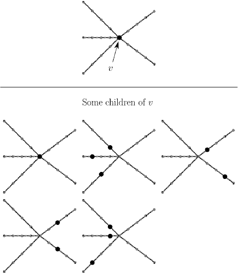
Figure 3.

Note that if $S\in\operatorname{PSlice}_{i}^{\prime}$ and $v_{1},v_{2}\in V_{i+1}$ are distinct vertices lying in $\pi_{i}^{-1}(S)$, then their trimmed stars are disjoint.

Definition 6.4.

If $S\in\operatorname{PSlice}_{i}^{\prime}$ is a partial slice, a child of $S$ is a subset $S^{\prime}\subset V_{i+1}^{\prime}$ obtained by replacing each vertex $v\in\pi_{i}^{-1}(S)\subset V_{i+1}$ with one of its children, so that $S^{\prime}$ is a subset of $V_{i+1}^{\prime}$. More formally, $S^{\prime}$ belongs to the image of the “union map”

$$\prod_{v\in\pi_{i}^{-1}(S)}\operatorname{Ch}(v)\longrightarrow V_{i+1}^{\prime}$$

which sends $\prod_{v}\,(S_{v})$ to $\cup_{v}\,S_{v}$. We use $\operatorname{Ch}(S)\subset\operatorname{PSlice}_{i+1}^{\prime}$ to denote the children of $S\in\operatorname{PSlice}_{i}^{\prime}$.

Lemma 6.5.

If $S$ is a partial slice, so is each of its children. Moreover, if $S\in\operatorname{Slice}_{i}^{\prime}$ is a slice, so is $S^{\prime}$.

Proof.

Suppose $S^{\prime}$ is a child of the partial slice $S\in\operatorname{PSlice}_{i}^{\prime}$, and $\gamma^{\prime}\subset X_{i+1}$ is a monotone geodesic. Then $\gamma^{\prime}$ projects isomorphically to a monotone geodesic $\gamma\subset X_{i}$, so $\pi_{i}^{-1}(S)\cap\gamma^{\prime}$ contains at most one vertex $v^{\prime}\in V_{i+1}$. From the definition of children, it follows that $\gamma^{\prime}\cap S^{\prime}$ contains at most one point. If $S$ is a slice, then $S^{\prime}$ contains precisely one vertex $v\in V_{i+1}^{\prime}$, and therefore $S^{\prime}$ contains a child of $\{v\}$, which will intersect $\gamma^{\prime}$ in precisely one point.

∎

Definition 6.6.

If $S\in\operatorname{PSlice}_{i}^{\prime}$ and $j>i$, then a partial slice $S^{\prime}\in\operatorname{PSlice}_{j}^{\prime}$ is a descendent of $S$ in $X_{j}^{\prime}$ if there exist $S=S_{i},S_{i+1},\ldots,S_{j}=S^{\prime}$ such that for all $k\in\{i+1,\ldots,j\}$, $S_{k}\in\operatorname{PSlice}_{k}^{\prime}$ and $S_{k}$ is a child of $S_{k-1}$; in other words, $S^{\prime}$ is an iterated child of $S$. We denote the collection of such descendents by $\operatorname{Desc}(S,X_{j}^{\prime})$.

Lemma 6.7.

For all $i<j$, if $S^{\prime}\in\operatorname{PSlice}_{j}^{\prime}$ is a descendent of $S\in\operatorname{PSlice}_{i}^{\prime}$, then $\pi_{i}(S^{\prime})\subset\cup_{w\in S}\operatorname{St}^{o}(w,X_{i}^{\prime})$.

Proof.

Suppose $S=S_{i},\ldots,S_{j}=S^{\prime}$, where $S_{k}\in\operatorname{PSlice}_{k}^{\prime}$ and $S_{k+1}$ is a child of $S_{k}$ for all $i\leq k<j$. Then

$$\pi_{k}(S_{k+1})\subset\pi_{k}\left(\cup_{w\in\pi_{k}^{-1}(S_{k})}\operatorname{TSt}(w,X_{k+1}^{\prime})\right)\,.$$

Iterating this yields the lemma. ∎

6.2. A measure on slices

We now define a measure on $\operatorname{Slice}_{i}^{\prime}$ for each $i$, by an iterated diffusion construction. To do this, we first associate with each vertex $v\in V_{i}$ a probability measure on its children $\operatorname{Ch}(v)\subset\operatorname{PSlice}_{i}^{\prime}$.

Definition 6.8.

If $v\in V_{i}$, let $w_{\operatorname{Ch}(v)}$ be the probability measure on $\operatorname{Ch}(v)$ which:

• Assigns measure $\frac{1}{m}$ to the child $\{v\}\in\operatorname{Ch}(v)$ of type (1).

• Uniformly distributes measure $\frac{1}{2}\cdot\frac{(m-1)}{m}$ among the children of type (2). Equivalently, for each vertex $\hat{v}\in V_{i}$ adjacent to $v$ with $v\prec\hat{v}$, we take the uniform measure on the $(m-1)$ vertices in $V_{i}^{\prime}$ which are interior points of the edge $\overline{v\hat{v}}$, take the product of these measures as $\hat{v}$ ranges over

  $$\{\bar{v}\in V_{i}\mid\bar{v}\in\operatorname{St}(v,X_{i}),\;v\prec\bar{v}\}\,$$

  and then multiply the result by $\frac{1}{2}\cdot\frac{(m-1)}{m}$.

• Uniformly distributes measure $\frac{1}{2}\cdot\frac{(m-1)}{m}$ among the children of type (3).

Note that if $v^{\prime}\in V_{i}^{\prime}$ belongs to the trimmed star of $v$, then the $w_{\operatorname{Ch}(v)}$ measure of the children of $v$ which contain $v^{\prime}$ is

(6.9) $$w_{\operatorname{Ch}(v)}(\{S\in\operatorname{Ch}(v)\mid v^{\prime}\in S\})=\begin{cases}\frac{1}{m}&\quad\mbox{if}\quad v^{\prime}=v\\ \frac{1}{2m}&\quad\mbox{if}\quad v^{\prime}\neq v\end{cases}$$

Using the measures $w_{\operatorname{Ch}(v)}$ we define a measure on the children of a slice:

Definition 6.10.

If $S\in\operatorname{Slice}_{i}^{\prime}$, we define a probability measure $K_{S}$ on $\operatorname{Ch}(S)$ as follows. We take the product measure $\prod_{v\in\pi_{i}^{-1}(S)}\,w_{\operatorname{Ch}(v)}$ on $\prod_{v\in\pi_{i}^{-1}(S)}\,\operatorname{Ch}(v)$, and push it forward under the union map

$$\prod_{v\in\pi_{i}^{-1}(S)}\,\operatorname{Ch}(v)\to\operatorname{Slice}_{i+1}^{\prime}\,.$$

In probabilistic language, for each $v\in\pi_{i}^{-1}(S)$, we independently choose a child of $v$ according to the distribution $w_{\operatorname{Ch}(v)}$, and then take the union of the resulting children. Note that this is well-defined because the inverse image of any slice is nonempty.

Now given a measure $\nu$ on $\operatorname{Slice}_{i}^{\prime}$, we diffuse it to a measure $\nu^{\prime}$ on $\operatorname{Slice}_{i+1}^{\prime}$:

(6.11) $$\nu^{\prime}=\sum_{S\in\operatorname{Slice}_{i}^{\prime}}\,K_{S}\,\nu(S)\,.$$

If we view the collection $\{K_{S}\}_{S\in\operatorname{Slice}_{i}^{\prime}}$ as defining a kernel

$$K_{i}:\operatorname{Slice}_{i}^{\prime}\times\operatorname{Slice}_{i+1}^{\prime}\to[0,1]$$

by the formula $K_{i}(S,S^{\prime})=K_{S}(S^{\prime})$, then the associated diffusion operator $K_{i}$ is given by

(6.12) $$K_{i}(\nu)(S^{\prime})=\sum_{S\in\operatorname{Slice}_{i}^{\prime}}K(S,S^{\prime})\nu(S)\,.$$

When $i<0$, then this sum will be finite for any measure $\nu$ since $K(S,S^{\prime})\neq 0$ for only finitely many $S$.

Lemma 6.13.

When $i\geq 0$, the sum will be finite provided $\nu$ is supported on the descendents of slices in $X_{0}^{\prime}$.

Proof.

For a given $S^{\prime}\in\operatorname{Slice}_{i+1}^{\prime}$, the summand $K(S,S^{\prime})\nu(S)$ is nonzero only if $S$ is a descendent of a slice $\{v\}\in V_{0}^{\prime}$ and $S^{\prime}$ is a child of $S$. By Lemma 6.7 this means that $\pi_{0}(S^{\prime})\subset\operatorname{St}^{o}(v,X_{0}^{\prime})$, so there are only finitely many possibilities for such $S$. ∎

Definition 6.14.

For $i\leq 0$, let $\Sigma_{i}^{\prime}$ the measure on $\operatorname{Slice}_{i}^{\prime}$ which assigns measure $m^{-(i+1)}$ to each slice in $\operatorname{Slice}_{i}^{\prime}=V_{i}^{\prime}$. For $i>0$ we define a measure $\Sigma_{i}^{\prime}$ on $\operatorname{Slice}_{i}^{\prime}$ inductively by $\Sigma_{i}^{\prime}=K_{i-1}(\Sigma_{i-1}^{\prime})$. This is well-defined by Lemma 6.13.

For every $S\in\operatorname{Slice}_{i}^{\prime}$ and every $j>i$, we may also obtain a well-defined probability measure on $\operatorname{Slice}_{j}^{\prime}$ which is supported on the descendents of $S$, by the formula

(6.15) $$K_{j-1}\circ\ldots\circ K_{i}(\delta_{S})\,,$$

where $\delta_{S}$ is a Dirac mass on $S$. Using this probability measure, we may speak of the measure of descendents of $S\in\operatorname{Slice}_{j}^{\prime}$.

7. Estimates on the family of measures $\{\Sigma_{i}^{\prime}\}_{i\in\mathbb{Z}}$

In this section we will prove (mostly by induction arguments) several estimates on the slice/cut measures $\{\Sigma_{i}^{\prime}\}$ and cut metrics $\{d_{\Sigma_{i}^{\prime}}\}$ that will be needed in Section 8.

We first observe that the slices passing through a vertex $v\in V_{i}^{\prime}$ have measure $m^{-(i+1)}$:

Lemma 7.1.

For all $i\in\mathbb{Z}$, and every $v\in V_{i}^{\prime}$, the $\Sigma_{i}^{\prime}$-measure of the collection of slices containing $v$ is precisely $m^{-(i+1)}$:

$$\Sigma_{i}^{\prime}(\{S\in\operatorname{Slice}_{i}^{\prime}\mid v\in S\})=m^{-(i+1)}\,.$$

Proof.

When $i\leq 0$ this reduces to the definition of $\Sigma_{i}^{\prime}$. So pick $i>0$, $v\in V_{i}^{\prime}$, and assume inductively that the lemma is true for $i-1$.

Case 1. $v\in V_{i}$. In this case, if a slice $S\in\operatorname{Slice}_{i-1}^{\prime}$ has a child $S^{\prime}\in\operatorname{Slice}_{i}^{\prime}$ containing $v$, then $\pi_{i-1}(v)\in S$. By Definition 6.8, for such an $S$, the fraction of its children containing $v$ is precisely $\frac{1}{m}$. Therefore by the induction hypothesis we have

$$\Sigma_{i}^{\prime}(\{S^{\prime}\mid v\in S^{\prime}\})=\frac{1}{m}\,\Sigma_{i-1}^{\prime}(\{S\in\operatorname{Slice}_{i-1}^{\prime}\mid\pi_{i-1}(v)\in S\})=m^{-(i+1)}\,.$$

Case 2. $v\not\in V_{i}$. Then $v$ belongs to a unique edge $\overline{w_{1}w_{2}}\subset X_{i}$, where $w_{1},w_{2}\in V_{i}$. In this case, a slice $S\in\operatorname{Slice}_{i-1}^{\prime}$ has a child $S^{\prime}\in\operatorname{Slice}_{i}^{\prime}$ containing $v$ if and only if $S$ contains $\pi_{i-1}(w_{1})$ or $\pi_{i-1}(w_{2})$. Since these possibilities are mutally exclusive (from the definition of slice), and each contributes a measure $\frac{1}{2}m^{-(i+1)}$ by the induction hypothesis and Definition 6.8, the lemma follows. ∎

Recall that by Lemma 6.2, for every $S\in\operatorname{Slice}_{i}^{\prime}$ the subset $S_{\leq}=\{x\in X_{i}\mid x\leq S\}$ is a monotone subset of $X_{i}$.

Definition 7.2.

Viewing $\Sigma_{i}^{\prime}$ as a cut measure on $X_{i}$ via the identification $S\longleftrightarrow S_{\leq}$, we let $d_{\Sigma_{i}^{\prime}}$ denote the corresponding cut metric on $X_{i}$. Equivalently, for $x_{1},x_{2}\in X_{i}$,

$$d_{\Sigma_{i}^{\prime}}(x_{1},x_{2})=\sum_{S\in\operatorname{Slice}_{i}^{\prime}}d_{S_{\leq}}(x_{1},x_{2})\,\Sigma_{i}^{\prime}(S)\,$$

where

$$d_{S_{\leq}}(x_{1},x_{2})= |\chi_{S_{\leq}}(x_{1})-\chi_{S_{\leq}}(x_{2})|$$

$$= \begin{cases}1&\quad\mbox{if}\quad x_{1}\preceq S\prec x_{2}\quad\mbox{or}\quad x_{2}\preceq S\prec x_{1}\\ 0&\quad\mbox{otherwise}\end{cases}$$

Lemma 7.3.

If $x_{1}^{\prime},x_{2}^{\prime}\in X_{i+1}$, and $\pi_{i}(x_{j}^{\prime})=x_{j}\in X_{i}$, then

(7.4) $$|d_{\Sigma_{i+1}^{\prime}}(x_{1}^{\prime},x_{2}^{\prime})-d_{\Sigma_{i}^{\prime}}(x_{1},x_{2})|\leq 4\,m^{-(i+1)}\,.$$

Proof.

For $j\in\{1,2\}$ let $S_{j}$ be the collection of slices $S\in\operatorname{Slice}_{i}^{\prime}$ which have a child $S^{\prime}\in\operatorname{Slice}_{i+1}^{\prime}$ such that $\operatorname{Side}(x_{j},S)\neq\operatorname{Side}(x_{j}^{\prime},S^{\prime})$. From the definition of children, it follows that if $S\in S_{j}$, then $x_{j}$ lies in $\operatorname{TSt}(v,X_{i}^{\prime})$ for some $v\in S$. Thus, if $\overline{w_{1}w_{2}}$ is an edge of $X_{i}^{\prime}$ containing $x_{j}$, then $S_{j}\subset\{S\in\operatorname{Slice}_{i}^{\prime}\mid S\cap\{w_{1},w_{2}\}\neq\emptyset\}$. By Lemma 7.1, we have $\Sigma_{i}^{\prime}(S_{j})\leq 2m^{-(i+1)}$. Now by the definition of the cut metrics, we get

$$|d_{\Sigma_{i+1}^{\prime}}(x_{1}^{\prime},x_{2}^{\prime})-d_{\Sigma_{i}^{\prime}}(x_{1},x_{2})|\leq\Sigma_{i}^{\prime}(S_{1}\cup S_{2})\leq 4\,m^{-(i+1)}\,.$$

∎

Lemma 7.5 (Persistence of sides).

Suppose $x\in X_{i}$, $S\in\operatorname{Slice}_{i}^{\prime}$, and $x\not\in\cup_{v\in S}\;\operatorname{St}^{o}(v,X_{i}^{\prime})$. Then for every $j\geq i$, every $x^{\prime}\in X_{j}$ with $\pi_{i}(x^{\prime})=x$, and for every descendent $S^{\prime}\in\operatorname{Slice}_{j}^{\prime}$ of $S$, we have

$$x^{\prime}\not\in\cup_{v\in S^{\prime}}\;\operatorname{St}^{o}(v,X_{j}^{\prime})\quad\mbox{and}\quad\operatorname{Side}(x^{\prime},S^{\prime})=\operatorname{Side}(x,S)\,.$$

Proof.

First suppose $j=i+1$. Then $x\notin\cup_{v\in\pi_{i}^{-1}(S)}\operatorname{St}^{o}(v,X_{i+1})$ because $\pi_{i}:X_{i+1}\to X_{i}^{\prime}$ is a simplicial mapping. Clearly this implies $\operatorname{Side}(x^{\prime},S^{\prime})=\operatorname{Side}(x^{\prime},\pi_{i+1}^{-1}(S))=\operatorname{Side}(x,S)$.

The $j>i+1$ case now follows by induction.

∎

Lemma 7.6 (Persistence of separation).

There is a constant $A=A(m)\in(0,1)$ with the following property. Suppose $j>i$, $x_{1},x_{2}\in X_{i}$, $x_{1}^{\prime},x_{2}^{\prime}\in X_{j}$, and $\pi_{i}(x_{1}^{\prime})=x_{1}$, $\pi_{i}(x_{2}^{\prime})=x_{2}$. Suppose in addition that

• $S\in\operatorname{Slice}_{i}^{\prime}$ is a slice which weakly separates $x_{1}$ and $x_{2}$.

• $x_{2}\notin\cup_{v\in S}\operatorname{St}^{o}(v,X_{i}^{\prime})$.

Then the measure of the collection of descendents $S^{\prime}\in\operatorname{Desc}(S,X_{j}^{\prime})$ which separate $x_{1}^{\prime}$ and $x_{2}^{\prime}$ is at least $A$; here we refer to the probability measure on $\operatorname{Desc}(S,X_{j})$ that was defined in equation (6.15).

Proof.

Since $S$ weakly separates $x_{1}$ and $x_{2}$ but $x_{2}\notin S$, without loss of generality we may assume that $x_{1}\preceq S\prec x_{2}$, since the case $x_{2}\prec S\preceq x_{1}$ is similar.

If $x_{1}\notin\cup_{v\in S}\operatorname{St}^{o}(v,X_{i}^{\prime})$, then by Lemma 7.5, for all $S^{\prime}\in\operatorname{Desc}(S,X_{j}^{\prime})$ we have $x_{1}^{\prime}\prec S^{\prime}\prec x_{2}^{\prime}$, so we are done in this case.

Therefore we assume that there exist $v\in S$ and $v^{\prime}\in\pi_{i}^{-1}(v)$ such that $x_{1}\in\operatorname{St}^{o}(v,X_{i}^{\prime})$, $x_{1}^{\prime}\in\operatorname{St}(v^{\prime},X_{i+1})$, and $x_{1}^{\prime}\preceq v^{\prime}$. If $S^{\prime}\in\operatorname{Slice}_{i+1}^{\prime}$ is a child of $S$ containing a child of $v^{\prime}$ of type (2), then $x_{1}^{\prime}\notin\cup_{w\in S^{\prime}}\operatorname{St}^{o}(w,X_{i+1}^{\prime})$; moreover the collection of such slices $S^{\prime}$ form a fraction at least $\frac{1}{2}\frac{m-1}{m}$ of the children of $S$. Applying Lemma 7.5 to each such slice $S^{\prime}$, we conclude that for every $S^{\prime\prime}\in\operatorname{Desc}(S^{\prime},X_{j}^{\prime})$, we have $x_{1}^{\prime}\prec S^{\prime\prime}\prec x_{2}^{\prime}$. This proves the lemma. ∎

Lemma 7.7.

Suppose $x_{1},x_{2}\in X_{i}$, $j>i$, $x_{1}^{\prime},x_{2}^{\prime}\in X_{j}$, $\pi_{i}(x_{1}^{\prime})=x_{1}$, $\pi_{i}(x_{2}^{\prime})=x_{2}$, and $\{x_{1},x_{2}\}$ is not contained in the trimmed star of any vertex $v\in V_{i}$. Then $d_{\Sigma_{j}^{\prime}}(x_{1}^{\prime},x_{2}^{\prime})\geq Am^{-(i+2)}$, where $A$ is the constant from Lemma 7.6.

Proof.

Choose $v_{1}\in V_{i}$ such that $x_{1}\in\operatorname{TSt}(v_{1},X_{i})$.

Observe that of the children $W$ of $v_{1}$, a measure at least $\frac{1}{2m}$ lie weakly on each side of $x_{1}$ and satisfy $x_{2}\notin\cup_{v\in W}\operatorname{St}^{o}(v,X_{i}^{\prime})$, in view of our assumption on $x_{1}$ and $x_{2}$, i.e.

$$w_{\operatorname{Ch}(v_{1})}\left(\{W\in\operatorname{Ch}(v_{1})\mid W\preceq x_{1},\;x_{2}\notin\cup_{v\in W}\operatorname{St}^{o}(v,X_{i}^{\prime})\}\right)\geq\frac{1}{2m}\,,$$

$$w_{\operatorname{Ch}(v_{1})}\left(\{W\in\operatorname{Ch}(v_{1})\mid W\succeq x_{1},\;x_{2}\notin\cup_{v\in W}\operatorname{St}^{o}(v,X_{i}^{\prime})\}\right)\geq\frac{1}{2m}\,.$$

Suppose $S\in\operatorname{Slice}_{i-1}^{\prime}$ and $v_{1}\in\pi_{i-1}^{-1}(S)$. Then each child $S^{\prime}\in\operatorname{Slice}_{i}^{\prime}$ of $S$ contains some child of $v_{1}$, and $\operatorname{Side}(x_{2},S^{\prime})$ is independent of this choice, because $x_{2}$ lies outside $\operatorname{TSt}(v_{1},X_{i})$. Furthermore, if $x_{2}\in\operatorname{St}(v_{2},X_{i})$ for some $v_{2}\in(V_{i}\cap\pi_{i-1}^{-1}(S))\setminus\{v_{1}\}$, then $S^{\prime}$ contains a child of $v_{2}$, and a fraction at least $\frac{1}{m}$ of this set of children $W\in\operatorname{Ch}(v_{2})$ satisfies $x_{2}\notin\cup_{v\in W}\operatorname{St}^{o}(v,X_{i}^{\prime})$. Thus a fraction at least $\frac{1}{2m^{2}}$ of the children of $S$ satisfy the assumptions of Lemma 7.6.

Since the set of $S\in\operatorname{Slice}_{i-1}^{\prime}$ with $v_{1}\in\pi_{i-1}^{-1}(S)$ has $\Sigma_{i-1}^{\prime}$-measure $m^{-i}$ by Lemma 7.1, by the preceding reasoning, we conclude that $d_{\Sigma_{j}^{\prime}}(x_{1}^{\prime},x_{2}^{\prime})\geq A\,m^{-(i+2)}$. ∎

Lemma 7.8.

Suppose $i,j\in\mathbb{Z}$, $i\leq j$, $x_{1},x_{2}\in X_{j}$, $e$ is an edge of $X_{i}$, and $\pi_{i}(x_{1}),\pi_{i}(x_{2})\in e$. Then

(7.9) $$d_{\Sigma_{j}^{\prime}}(x_{1},x_{2})\leq m^{-i}\,.$$

Proof.

Let $v_{1},v_{2}$ be the endpoints of $e$, where $v_{1}\prec v_{2}$. We may assume without loss of generality that $\pi_{i}(x_{1})\preceq\pi_{i}(x_{2})$.

By Definition 7.2, the distance $d_{\Sigma_{j}^{\prime}}(x_{1},x_{2})$ is the $\Sigma_{j}^{\prime}$-measure of the set

$$Y=\{S\in\operatorname{Slice}_{j}^{\prime}\mid\;x_{1}\preceq S\prec x_{2}\quad\mbox{or}\quad x_{2}\preceq S\prec x_{1}\;\}.$$

If $S\in\operatorname{Slice}_{i}^{\prime}$ and $S\cap e=\emptyset$, then $S$ does not weakly separate $\pi_{i}(x_{1}),\pi_{i}(x_{2})$, so by Lemma 7.5, no descendent $S^{\prime}\in\operatorname{Desc}(S,X_{j}^{\prime})$ can weakly separate $x_{1}$ and $x_{2}$, i.e. $Y\cap\operatorname{Desc}(S,X_{j}^{\prime})=\emptyset$. For $v\in V_{i}^{\prime}$ let

$$\operatorname{Slice}_{i}^{\prime}(v)=\{S\in\operatorname{Slice}_{i}^{\prime}\mid v\in S\}\,$$

and let $\Sigma_{i}^{\prime}\>\mbox{\rule{0.43057pt}{5.16663pt}\rule{8.1805pt}{0.43057pt}}\>\operatorname{Slice}_{i}^{\prime}(v)$ be the restriction of $\Sigma_{i}^{\prime}$ to $\operatorname{Slice}_{i}^{\prime}(v)$. Thus, using the diffusion operators $K_{l}$ from (6.11), the above observation implies that

$$\Sigma_{j}^{\prime}(Y)= K_{j-1}\circ\ldots\circ K_{i}(\Sigma_{i}^{\prime})(Y)$$

$$= \sum_{v\in e\cap V_{i}^{\prime}}K_{j-1}\circ\ldots\circ K_{i}(\Sigma_{i}^{\prime}\>\mbox{\rule{0.43057pt}{5.16663pt}\rule{8.1805pt}{0.43057pt}}\>\operatorname{Slice}_{i}^{\prime}(v))(Y)$$

(7.10) $$\quad\quad\leq(m-1)m^{-(i+1)}+\sum_{v\in\{v_{1},v_{2}\}}K_{j-1}\circ\ldots\circ K_{i}(\Sigma_{i}^{\prime}\>\mbox{\rule{0.43057pt}{5.16663pt}\rule{8.1805pt}{0.43057pt}}\>\operatorname{Slice}_{i}^{\prime}(v))(Y)\,,$$

because the mass of $\Sigma_{i}^{\prime}\>\mbox{\rule{0.43057pt}{5.16663pt}\rule{8.1805pt}{0.43057pt}}\>\operatorname{Slice}_{i}^{\prime}(v)$ is $m^{-(i+1)}$ by Lemma 7.1. The remainder of the proof is devoting to showing that the total contribution from the last two terms in (7.10) is at most $m^{-(i+1)}$.

Suppose $\pi_{i}(x_{1})\notin\operatorname{St}^{o}(v_{1},X_{i}^{\prime})$. If $S\in\operatorname{Slice}_{i}^{\prime}(v_{1})$, then no descendent $S^{\prime}\in\operatorname{Desc}(S,X_{j}^{\prime})$ can weakly separate $x_{1},x_{2}$ by Lemma 7.5. Therefore

$$K_{j-1}\circ\ldots\circ K_{i}(\Sigma_{i}^{\prime}\>\mbox{\rule{0.43057pt}{5.16663pt}\rule{8.1805pt}{0.43057pt}}\>\operatorname{Slice}_{i}^{\prime}(v_{1}))(Y)=0\,,$$

so we are done in this case. Hence we may assume that $\pi_{i}(x_{1})\in\operatorname{St}^{o}(v_{1},X_{i}^{\prime})$, and by similar reasoning, that $\pi_{i}(x_{2})\in\operatorname{St}^{o}(v_{2},X_{i}^{\prime})$. This implies by Lemma 7.5 that if $v_{1}\in S\in\operatorname{Slice}_{i}^{\prime}$ and $S^{\prime}\in\operatorname{Desc}(S,X_{j}^{\prime})$ then $S^{\prime}\prec x_{2}$; similarly, if $v_{2}\in S\in\operatorname{Slice}_{i}^{\prime}$ and $S^{\prime}\in\operatorname{Desc}(S,X_{j}^{\prime})$, then $x_{1}\prec S^{\prime}$.

By (7.10), the lemma now reduces to the following two claims:

Claim 1. $K_{j-1}\circ\ldots\circ K_{i}(\Sigma_{i}^{\prime}\>\mbox{\rule{0.43057pt}{5.16663pt}\rule{8.1805pt}{0.43057pt}}\>\operatorname{Slice}_{i}^{\prime}(v_{1}))(Y)\leq\frac{1}{2}(m^{-(i+1)}+m^{-(j+1)})$.

Claim 2. $K_{j-1}\circ\ldots\circ K_{i}(\Sigma_{i}^{\prime}\>\mbox{\rule{0.43057pt}{5.16663pt}\rule{8.1805pt}{0.43057pt}}\>\operatorname{Slice}_{i}^{\prime}(v_{2}))(Y)\leq\frac{1}{2}(m^{-(i+1)}-m^{-(j+1)})$.

Proof of Claim 1. For each $i\leq k\leq j$, let $w_{k}^{\prime}$ be the unique vertex in $V_{k}^{\prime}$ such that $\pi_{k}(x_{1})\in\operatorname{St}^{o}(w_{k}^{\prime},X_{k}^{\prime})$ and $w_{k}^{\prime}\preceq\pi_{k}(x_{1})$. Likewise, let $w_{k}$ be the unique vertex in $V_{k}$ such that $\pi_{k}(x_{1})\in\operatorname{St}^{o}(w_{k},X_{k})$ and $w_{k}\preceq\pi_{k}(x_{1})$. Thus $w_{k}^{\prime}\in\operatorname{St}^{o}(w_{k},X_{k})$. Let $k_{0}$ be the maximum of the integers $k\in[i,j]$ such that $\pi_{i}(w_{\bar{k}}^{\prime})=v_{1}$ for all $i\leq\bar{k}\leq k$. It follows that $w_{k}^{\prime}=w_{k}$ for all $i\leq k\leq k_{0}$.

For $i\leq k\leq j$, let $A_{k}$ be the collection of slices $S\in\operatorname{Slice}_{k}^{\prime}$ which contain $w_{k}$, and let $B_{k}$ be the collection of slices $S\in\operatorname{Slice}_{k}^{\prime}$ which contain a child of $w_{k}$ of type (3). We now define a sequence of measures $\{\alpha_{k}\}_{i\leq k\leq k_{0}}$ inductively as follows. Let $\alpha_{i}$ be the restriction of $\Sigma_{i}^{\prime}$ to $\{S\in\operatorname{Slice}_{i}^{\prime}\mid v_{1}\in S\}$. For $k<k_{0}$, we define $\alpha_{k+1}$ to the restriction of $K_{k}\alpha_{k}$ to $\operatorname{Slice}_{k+1}^{\prime}\setminus B_{k+1}$, where $K_{k}$ is the diffusion operator (6.11). Since by Lemma 7.5 the set of descendents $\operatorname{Desc}(B_{k},X_{j}^{\prime})$ is disjoint from $Y$, it follows that

(7.11) $$\quad\quad K_{j-1}\circ\ldots\circ K_{i}(\Sigma_{i}^{\prime}\>\mbox{\rule{0.43057pt}{5.16663pt}\rule{8.1805pt}{0.43057pt}}\>\operatorname{Slice}_{i}^{\prime}(v_{1}))\>\mbox{\rule{0.43057pt}{5.16663pt}\rule{8.1805pt}{0.43057pt}}\>Y=(K_{j-1}\circ\ldots K_{k}\alpha_{k})\>\mbox{\rule{0.43057pt}{5.16663pt}\rule{8.1805pt}{0.43057pt}}\>Y$$

for all $k\leq k_{0}$.

Note that by the definition of the diffusion operator $K_{k-1}$ we have

(7.12) $$\alpha_{k}(A_{k})\geq \frac{1}{m}\cdot\alpha_{k-1}(A_{k-1})$$

(7.13) $$(K_{k-1}\alpha_{k-1})(B_{k})\geq \frac{(m-1)}{2m}\cdot\alpha_{k-1}(A_{k-1})$$

for all $i<k\leq k_{0}$. This yields $\alpha_{k}(A_{k})\geq m^{-(k+1)}$ for all $i\leq k\leq k_{0}$. Hence for all $i<k\leq k_{0}$ we get

$$\alpha_{k}(\operatorname{Slice}_{k}^{\prime})= \,\alpha_{k-1}(\operatorname{Slice}_{k-1}^{\prime})-(K_{k-1}\alpha_{k-1})(B_{k})$$

$$\leq \,\alpha_{k-1}(\operatorname{Slice}_{k-1}^{\prime})-\frac{(m-1)}{2m}\cdot m^{-k}$$

and so

$$\alpha_{k_{0}}(\operatorname{Slice}_{k_{0}}^{\prime})\leq m^{-(i+1)}-\frac{(m-1)}{2m}\cdot(m^{-(i+1)}+\ldots+m^{-k_{0}})$$

$$= \frac{1}{2}m^{-(i+1)}+\frac{1}{2}m^{-(k_{0}+1)}\,.$$

This gives Claim 1 when $k_{0}=j$, by (7.11).

We now assume that $k_{0}<j$. Then $w_{k_{0}+1}\prec w_{k_{0}+1}^{\prime}$. By Lemma 7.5, every descendent $S^{\prime}\in\operatorname{Slice}_{j}^{\prime}$ of a slice $S\in A_{k_{0}+1}\cup B_{k_{0}+1}$ will satisfy $S^{\prime}\prec x_{1}$, so $S^{\prime}\notin Y$. Therefore if we define $\alpha_{k_{0}+1}$ to be the restriction of $K_{k_{0}}\alpha_{k_{0}}$ to $\operatorname{Slice}_{k_{0}+1}^{\prime}\setminus(A_{k_{0}+1}\cup B_{k_{0}+1})$, then

$$K_{j-1}\circ\ldots\circ K_{i}(\Sigma_{i}^{\prime}\>\mbox{\rule{0.43057pt}{5.16663pt}\rule{8.1805pt}{0.43057pt}}\>\operatorname{Slice}_{i}^{\prime}(v_{1}))(Y)=K_{j-1}\circ\ldots\circ K_{k_{0}+1}(\alpha_{k_{0}+1})(Y)\,.$$

Also, as in (7.12)–(7.13), we get

$$K_{k_{0}}\alpha_{k_{0}}(A_{k_{0}+1}\sqcup B_{k_{0}+1})\geq \left(\frac{1}{m}+\frac{(m-1)}{2m}\right)\alpha_{k_{0}}(A_{k_{0}})$$

$$\geq \left(\frac{1}{m}+\frac{(m-1)}{2m}\right)m^{-(k_{0}+1)}\,.$$

Therefore

$$K_{j-1}\circ\ldots\circ K_{k_{0}+1}(\alpha_{k_{0}+1})(Y)\leq \;\alpha_{k_{0}+1}(\operatorname{Slice}_{k_{0}+1}^{\prime})$$

$$= \;\alpha_{k_{0}}(\operatorname{Slice}_{k_{0}}^{\prime})-K_{k_{0}}\alpha_{k_{0}}(A_{k_{0}+1}\sqcup B_{k_{0}+1})$$

$$\leq \;\frac{1}{2}m^{-(i+1)}+\frac{1}{2}m^{-(k_{0}+1)}-\left(\frac{1}{m}+\frac{(m-1)}{2m}\right)m^{-(k_{0}+1)}$$

$$\leq \;\frac{1}{2}m^{-(i+1)}-\frac{1}{2}m^{-(k_{0}+1)}$$

so Claim 1 holds.

Proof of Claim 2. The proof is similar to that of Claim 1, except that one replaces $v_{1}$ with $v_{2}$, and reverses the orderings. However, in the case when $k_{0}=j$, one simply notes that any slice $S^{\prime}\in A_{k_{0}}=A_{j}$ satisfies $x_{1}\preceq S^{\prime}$, $x_{2}\preceq S^{\prime}$, so $S^{\prime}\notin Y$. Therefore we may remove the measure contributed by $A_{k_{0}}$ from our estimate, making it smaller by $m^{-(j+1)}$.

∎

Corollary 7.14.

Suppose $i,j\in\mathbb{Z}$, $i\leq j$, $x_{1},x_{2}\in X_{j}$, $v\in V_{i}$, and $\{x_{1},x_{2}\}\subset(\pi_{i}^{j})^{-1}(\operatorname{St}(v,X_{i}))$. Then

(7.15) $$d_{\Sigma_{j}^{\prime}}(x_{1},x_{2})\leq 2m^{-i}\,.$$

Proof.

First suppose there is an $x\in X_{j}$ such that $\pi_{i}^{j}(x)=v$. Then $\{\pi_{i}^{j}(x),\pi_{i}^{j}(x_{1})\}$ lies in an edge of $X_{i}$, so by Lemma 7.8 we have $d_{\Sigma_{j}^{\prime}}(x,x_{1})\leq m^{-i}$, and similarly $d_{\Sigma_{j}^{\prime}}(x,x_{2})\leq m^{-i}$. Therefore (7.15) holds.

In general, construct a new admissible inverse system $\{Y_{k}\}$ satisfying Assumption 5.1 by letting $Y_{k}$ be the disjoint union of $X_{k}$ with a copy of $\mathbb{R}$ when $i<k\leq j$, and $Y_{k}=X_{k}$ otherwise. Then extend the projection map $\pi_{i}:X_{i+1}\to X_{i}$ to $\pi_{i}:Y_{i+1}\to Y_{i}=X_{i}$ by mapping $Y_{i+1}\setminus X_{i+1}\simeq\mathbb{R}$ to a monotone geodesic containing $v$. Then for $i<k<j$ extend $\pi_{j}:X_{j+1}\to X_{j}$ to $\pi_{j}:Y_{j+1}\to Y_{j}$ by mapping $Y_{j+1}\setminus X_{j+1}\simeq\mathbb{R}$ isomorphically to $Y_{j}\setminus X_{j}\simeq\mathbb{R}$. Then there is a system of measures $\{\Sigma_{k,Y}^{\prime}\}$ for the inverse system $\{Y_{k}\}$, and it follows that the associated cut metric $d_{\Sigma_{j}^{\prime}}^{Y}$ is the same for pairs $x_{1},x_{2}\subset X_{j}\subset Y_{j}$. Since $v$ belongs to the image of $\pi_{i}^{j}:Y_{j}\to Y_{i}$, we have $d_{\Sigma_{j}^{\prime}}^{X}(x_{1},x_{2})=d_{\Sigma_{j}^{\prime}}^{Y}(x_{1},x_{2})\leq 2m^{-i}$. ∎

8. Proof of Theorem 1.16 under Assumption 5.1

We will define a sequence $\{\rho_{i}:X_{\infty}\times X_{\infty}\to[0,\infty)\}$ of pseudo-distances on $X_{\infty}$, such that $\rho_{i}$ is induced by a map $X_{\infty}\to L_{1}$, and $\rho_{i}$ converges uniformly to some $\rho_{\infty}:X_{\infty}\times X_{\infty}\to[0,\infty)$. By a standard argument, this yields an isometric embedding $(X_{\infty},\rho_{\infty})\to L_{1}$. (The theory of ultralimits [HM82, BL00] implies the metric space $(X_{\infty},\rho_{\infty})$ isometrically embeds in an ultralimit $V$ of $L_{1}$ spaces; by Kakutani’s theorem [Kak39] the space $V$ is isometric to an $L_{1}$ space, and so $\rho_{\infty}$ isometrically embeds in $L_{1}$.) To complete the proof, it suffices to verify that $\rho_{\infty}$ has the properties asserted by the theorem. (Alternately, one may construct a cut measure $\Sigma_{\infty}$ on $X_{\infty}$ as weak limit, and use the corresponding cut metric to provide the embedding to $L_{1}$.)

Let $\rho_{i}=(\pi_{i}^{\infty})^{*}d_{\Sigma_{i}^{\prime}}$ be the pullback of $d_{\Sigma_{i}^{\prime}}$ to $X_{\infty}$. By Lemma 7.3 we have $|\rho_{i+1}-\rho_{i}|\leq 4\,m^{-(i+1)}$, so the sequence $\{\rho_{i}\}$ converges uniformly to a pseudo-distance $\rho_{\infty}:X_{\infty}\times X_{\infty}\to[0,\infty)$.

Lemma 8.1.

1. $\rho_{\infty}(x,x^{\prime})\leq\bar{d}_{\infty}(x,x^{\prime})$.

2. $\rho_{\infty}(x,x^{\prime})\geq\frac{A}{2m^{3}}\cdot\bar{d}_{\infty}(x,x^{\prime})\,.$

3. $\rho_{\infty}(x,x^{\prime})=\bar{d}_{\infty}(x,x^{\prime})$ if $x,x^{\prime}$ lie on a monotone geodesic.

Proof.

(1). Suppose $x,x^{\prime}\in X_{\infty}$, and for some $i\in\mathbb{Z}$ the projections $\{\pi_{i}(x),\pi_{i}(x^{\prime})\}$ are contained in $\operatorname{St}(v,X_{i})$. By Corollary 7.14 we have $\rho_{\infty}(x,x^{\prime})\leq 2m^{-i}$. Now (1) follows from the definition of $\bar{d}_{\infty}$.

(2). Suppose $x\neq x^{\prime}$, and let $j\in\mathbb{Z}$ be the minimum of the indices $k\in\mathbb{Z}$ such that $\pi_{k}(x),\pi_{k}(x^{\prime})$ are not contained in the trimmed star of any vertex $v\in X_{k}$. Then $\bar{d}_{\infty}(x,x^{\prime})\leq 2m^{-(j-1)}$ by Lemma 2.6, while $\rho_{\infty}(x,x^{\prime})\geq Am^{-(j+2)}$ by Lemma 7.7. Thus

$$\rho_{\infty}(x,x^{\prime})\geq\frac{A}{2m^{3}}\cdot\bar{d}_{\infty}(x,x^{\prime})\,.$$

(3). If $x,x^{\prime}\in X_{\infty}$ lie on a monotone geodesic $\gamma$, then $\gamma$ will project homeomorphically under $\pi_{i}$ to a monotone geodesic $\pi_{i}(\gamma)$, which contains at least $\bar{d}_{\infty}(x_{1},x_{2})m^{(i+1)}-2$ vertices of $V_{i}^{\prime}$. By Lemma 7.1 we have $\rho_{i}(x_{1},x_{2})\geq\bar{d}_{\infty}(x_{1},x_{2})-2m^{-(i+1)}$. Since $i$ was arbitrary we get $\rho_{\infty}(x,x^{\prime})=\bar{d}_{\infty}(x,x^{\prime})$. ∎

This completes the proof of Theorem 1.16 under Assumption 5.1.

9. The proof of Theorem 1.16, general case

We recall the three conditions from Assumption 5.1:

1. $\pi_{i}$ is finite-to-one for all $i\in\mathbb{Z}$.

2. $X_{i}\simeq\mathbb{R}$ and $\pi_{i}:X_{i+1}\to X_{i}^{\prime}$ is an isomorphism for all $i\leq 0$.

3. For every $i\in\mathbb{Z}$, every vertex $v\in V_{i}$ has neighbors $v_{\pm}\in V_{i}$ with $v_{-}\prec v\prec v_{+}$. Equivalently, $X_{i}$ is a union of monotone geodesics (see Definition 2.12).

In this section these three conditions will be removed in turn.

9.1. Removing the finiteness assumption

We now assume that $\{X_{i}\}$ is an admissible inverse system satisfying conditions (2) and (3) of Assumption 5.1, but not necessarily the finiteness condition (1).

To prove Theorem 1.16 without the finiteness assumption, we observe that the construction of the distance function $\rho_{\infty}:X_{\infty}\times X_{\infty}\to\mathbb{R}$ can be reduced to the case already treated, in the sense that for any two points $x_{1},x_{2}\in X_{\infty}$, we can apply the construction of the cut metrics to finite valence subsystems, and the resulting distance $\rho_{\infty}(x_{1},x_{2})$ is independent of the choice of subsystem. The proof is then completed by invoking the main result of [DCK72]. We now give the details.

Definition 9.1.

A finite subsystem of the inverse system $\{X_{j}\}$ is a collection of subcomplexes $\{Y_{j}\subset X_{j}\}_{j=-\infty}^{i}$, for some $i\geq 0$, such that $\pi_{j}(Y_{j+1})\subset Y_{j}$ for all $j<i$, and $\{Y_{j}\}_{j\leq i}$ satisfies Assumption 5.1 for indices $\leq i$. In other words:

1. $\pi_{j}$ is finite-to-one for all $j\leq i$.

2. $Y_{j}\simeq\mathbb{R}$ and $\pi_{j}:Y_{j+1}\to Y_{j}^{\prime}$ is an isomorphism for all $j\leq 0$.

3. $Y_{j}$ is a union of (complete) monotone geodesics for all $j\leq i$.

Suppose $i\geq 0$ and $V$ is a finite subset of $V_{i}^{\prime}\subset X_{i}$. Then there exists a finite subsystem $\{Y_{j}\}_{j=-\infty}^{i}$ such that $Y_{i}$ contains $V$. One may be obtain such a system by letting $Y_{i}$ be a finite union of monotone geodesics in $X_{i}$ which contains $V$, and taking $Y_{j}=\pi_{j}^{i}(Y_{i})$ for $j<i$. The inductive construction of the slice measures in the finite valence case may be applied to the finite subsystem $\{Y_{j}\}$, to obtain a sequence of slice measures which we denote by $\Sigma_{j,Y}^{\prime}$, to emphasize the potential dependence on $Y$.

Lemma 9.2.

Suppose $i\geq 0$, $V\subset V_{i}^{\prime}$ is a finite subset, and let $\{Y_{j}\}_{j\leq i_{Y}}$ and $\{Z_{j}\}_{j\leq i_{Z}}$ be finite subsystems of $\{X_{j}\}$, where $i\leq\min(i_{Y},i_{Z})$ and $V\subset Y_{i}\cap Z_{i}$. If $\Sigma_{i,Y}^{\prime}$, $\Sigma_{i,Z}^{\prime}$ denote the respective slice measures, then

$$\Sigma_{i,Y}^{\prime}(\{S\in\operatorname{Slice}_{i,Y}^{\prime}\mid S\supset V\})=\Sigma_{i,Z}^{\prime}(\{S\in\operatorname{Slice}_{i,Z}^{\prime}\mid S\supset V\})\,,$$

i.e. the slice measure does not depend on the choice of subsystem containing $V$.

Proof.

If $i\leq 0$ then $Y_{i}=Z_{i}$ and $\Sigma_{i,Y}^{\prime}=\Sigma_{i,Z}^{\prime}$ by construction. So assume that $i>0$, and that the lemma holds for all finite subsets of $V_{\bar{i}}^{\prime}$ for all $\bar{i}<i$.

Suppose $S^{\prime}\in\operatorname{Slice}_{i,Y}^{\prime}$ is a child of $S\in\operatorname{Slice}_{i-1,Y}^{\prime}$, and $V\subset S^{\prime}$. Then for every $v\in V$, either $v\in V_{i}$, in which case $\pi_{i-1}(v)\in S$, or $v\in V_{i}^{\prime}\setminus V_{i}$, in which case $v$ is an interior point of some edge $\overline{u_{1}u_{2}}$ of $Y_{i}\subset X_{i}$, and $S$ contains precisely one of the points $\pi_{i-1}(u_{1})$, $\pi_{i-1}(u_{2})$. By the definition of $\Sigma_{i,Y}^{\prime}$ given by (6.11):

$$\Sigma_{i,Y}^{\prime}(\{S^{\prime} \in\operatorname{Slice}_{i,Y}^{\prime}\mid S^{\prime}\supset V\})$$

(9.3) $$= \sum_{S\in\operatorname{Slice}_{i-1,Y}^{\prime}}\,K_{S}(\{S^{\prime}\in\operatorname{Slice}_{i,Y}^{\prime}\mid S^{\prime}\supset V\})\,\Sigma_{i-1,Y}^{\prime}(S)$$

By the above observation, the nonzero terms in the sum come from the slices $S\in\operatorname{Slice}_{i-1,Y}^{\prime}$ which contain precisely one of a finite collection of finite subsets $\bar{V}_{1},\ldots,\bar{V}_{k}\subset V_{i-1}^{\prime}$. If $S\in\operatorname{Slice}_{i-1,Y}^{\prime}$ contains $\bar{V}_{l}$, then from the definition of $K_{S}$, the quantity $K_{S}(\{S^{\prime}\in\operatorname{Slice}_{i}^{\prime}\mid S^{\prime}\supset V\})$ depends only on $V_{l}$. Therefore by the induction assumption, it follows that the nonzero terms in (9.1) will be the same as the corresponding terms in the sum defining $\Sigma_{i,Z}(\{S^{\prime}\in\operatorname{Slice}_{i,Y}^{\prime}\mid S^{\prime}\supset V\})$.

∎

Lemma 9.4.

If $\{Y_{j}\}_{j\leq i}$ is a finite subsystem such that $Y_{i}$ contains $\{x_{1},x_{2}\}\subset X_{i}$, then the cut metric $d_{\Sigma_{i,Y}^{\prime}}(x_{1},x_{2})$ does not depend on the choice of $\{Y_{j}\}_{j\leq i}$.

Proof.

Let $\gamma_{1},\gamma_{2}\subset Y_{i}$ be monotone geodesics containing $x_{1}$ and $x_{2}$ respectively. Then $d_{\Sigma_{i,Y}^{\prime}}(x_{1},x_{2})$ is the total $\Sigma_{i,Y}^{\prime}$-measure of the slices $S\in\operatorname{Slice}_{i,Y}^{\prime}$ such that either $x_{1}\preceq S\prec x_{2}$ or $x_{2}\preceq S\prec x_{1}$. But every such slice $S$ contains precisely one point from $\gamma_{1}$, and one point from $\gamma_{2}$. As the choice of $\gamma_{1}$, $\gamma_{2}$ was arbitrary, Lemma 9.2 implies that cut metric $d_{\Sigma_{i,Y}^{\prime}}(x_{1},x_{2})$ does not change when we pass from $\{Y_{j}\}_{j\leq i}$ to another subsystem which contains $\{Y_{j}\}_{j\leq i}$. This implies the lemma, since the union of any two finite subsystems containing $\{x_{1},x_{2}\}$ is a finite subsystem which assigns the same cut metric to $(x_{1},x_{2})$. ∎

We now define a sequence of pseudo-distances $\{\rho_{i}:X_{\infty}\times X_{\infty}\to[0,\infty)$ by letting $\rho_{i}(x_{1},x_{2})=d_{\Sigma_{i,Y}}(\pi_{i}^{\infty}(x_{1}),\pi_{i}^{\infty}(x_{2}))$ where $\{Y_{j}\}_{j\leq i}$ is any finite subsystem containing $\{\pi_{i}^{\infty}(x_{1}),\pi_{i}^{\infty}(x_{2})\}$. By Lemma 9.4 the pseudo-distance is well-defined. As in the finite valence case:

• Lemma 7.3 implies that $\{\rho_{i}\}$ converges uniformly to a pseudo-distance $\rho_{\infty}:X_{\infty}\times X_{\infty}\to[0,\infty)$.

• $\frac{A}{2m^{3}}\bar{d}_{\infty}\leq\rho_{\infty}\leq\bar{d}_{\infty}$, since this may be verified for each pair of points $x_{1},x_{2}\in X_{\infty}$ at a time, by using finite subsystems.

• If $V\subset X_{\infty}$ is a finite subset, then the restriction of $\rho_{i}$ to $V$ embeds isometrically in $L_{1}$ for all $i$, and hence the same is true for $\rho_{\infty}$.

By the main result of [DCK72], if $Z$ is a metric space such that every finite subset isometrically embeds in $L_{1}$, then $Z$ itself isometrically embeds in $L_{1}$. Therefore $(X_{\infty},\rho_{\infty})$ isometrically embeds in $L_{1}$.

9.2. Removing Assumption 5.1(2)

Now suppose $\{X_{i}\}$ is an admissible inverse system satisfying Assumption 5.1(3), i.e. it is a union of monotone geodesics. We will reduce to the case treated in Section 9.1 by working with balls, and then take an ultralimit as the radius tends to infinity.

Lemma 9.5.

Suppose $p\in X_{\infty}$, $R\in(0,\infty)$ and $R<m^{-(i+1)}$. Then there is an admissible inverse system $\{Z_{j}\}$ satisfying (2) and (3) of Assumption 5.1, and an isometric embedding of the rescaled ball:

$$\phi:(B(p,R),m^{(i-1)}\bar{d}_{\infty})\to Z_{\infty}$$

which preserves the partial order, i.e. if $x,y\in B(p,R)$ and $x\preceq y$, then $\phi(x)\preceq\phi(y)$.

Proof.

Since $R<m^{-(i+1)}$, by Lemma 2.4 there is a $v\in V_{i}$ such that $\pi_{i}(B(p,R))\subset\operatorname{TSt}(v,X_{i})$.

We now construct an inverse system $\{Y_{j}\}$ as follows. For $j\geq i$, we let $Y_{j}$ be the inverse image of $\operatorname{St}(v,X_{i})$ under the projection $\pi_{i}^{j}:X_{j}\to X_{i}$. We let $Y_{j}\simeq\mathbb{R}$ for $j<i$. To define the projection maps, we take $\pi_{j}^{Y}=\pi_{i}^{X}\mbox{\Large$|$\normalsize}_{Y_{j+1}}$ for $j\geq i$, and let $\pi_{j}^{Y}:Y_{j+1}\to Y_{j}^{\prime}$ be a simplicial isomorphism for $j<i-1$. Finally, we take $\pi_{i-1}^{Y}:Y_{i}=\operatorname{St}(v,X_{j})\to Y_{i-1}^{\prime}\simeq\mathbb{R}$ to be an order preserving simplicial map which is an isomorphism on edges, thus the star $Y_{i}=\operatorname{St}(v,X_{i})$ is collapsed onto two consecutive edges $\overline{w_{-}w}$, $\overline{ww_{+}}$ in $Y_{i-1}^{\prime}$, where $w=\pi_{i-1}(v)$, $w_{-}\prec w$, and $w\prec w_{+}$. Thus $\{Y_{j}\}$ is an admissible inverse system, but it need not satisfy (2) or (3) of Assumption 5.1.

Next, we enlarge $\{Y_{j}\}$ to a system $\{\hat{Y}_{j}\}$. We first attach, for every $k\geq i$, and every vertex $z\in(\pi_{i-1}^{k})^{-1}(w_{-})$, a directed ray $\gamma_{z}$ which is directed isomorphic to $(-\infty,0]$ with the usual subdivision and order. We then extend the projection maps so that if $\pi_{k}(z)=z^{\prime}$ then $\gamma_{z}\subset Y_{j+1}$ is mapped direction-preserving isomorphically to a ray in $X_{j}^{\prime}$ starting at $z^{\prime}$. Then similarly, we attach directed rays to vertices $z\in(\pi_{i-1}^{k})^{-1}(w_{+})$, and extend the projection maps.

Finally, we let $\{Z_{j}\}$ be the system obtained from $\{\hat{Y}_{j}\}$ by shifting indices by $(i-1)$, in other words $Z_{j}=Y_{j-i-1}$.

Then $\{Z_{j}\}$ satisfies (2) and (3) of Assumption 5.1. For all $j\geq i$, we have compatible direction preserving simpliicial embeddings $X_{j}\supset(\pi_{i}^{j})^{-1}(\operatorname{St}(v,X_{i}))\to Z_{j-i+1}$. We will identify points with their image under this embedding. If $x,x^{\prime}\in B(p,R)$ and $x=x_{0},\ldots,x_{k}=x^{\prime}$ is a chain of points as in Lemma 2.3 which nearly realizes $\bar{d}_{\infty}^{X}(x,x^{\prime})$, then the chain and the associated stars will project into $\operatorname{St}(v,X_{i})$; this implies that $\bar{d}_{\infty}^{Z}(x,x^{\prime})\leq m^{(i-1)}\bar{d}_{\infty}^{X}(x,x^{\prime})$. Similar reasoning gives $m^{(i-1)}\bar{d}_{\infty}^{X}(x,x^{\prime})\leq\bar{d}_{\infty}^{Z}(x,x^{\prime})$.

If $\gamma\subset B(p,R)$ is a monotone geodesic segment, then $\pi_{i}(\gamma)$ is a monotone geodesic segment in $\operatorname{St}(v,X_{i})$ with endpoints in $\operatorname{St}(v,X_{i})$, and so $\pi_{i}(\gamma)\subset\operatorname{St}(v,X_{i})$. Thus the embedding also preserves the partial order as claimed.

∎

Fix $p\in X_{\infty}$. Then for every $n\in\mathbb{N}$, since $m^{n}<m^{(n+1)}$, Lemma 9.5 provides an inverse system $\{Z_{j}^{n}\}_{j\in\mathbb{Z}}$ and an embedding

$$\phi_{n}:(B(p,m^{n}),m^{-n-3}\bar{d}_{\infty})\to Z_{\infty}^{n}\,.$$

Let $f_{n}:Z_{\infty}^{n}\to L_{1}$ be a $1$-Lipschitz embedding satisfying the conclusion of Theorem 1.16, constructed in Section 9.1, and let $\psi_{n}:(B(p,m^{n}),\bar{d}_{\infty})\to L_{1}$ be the composition $f_{n}\circ\phi_{n}$, rescaled by $m^{n+3}$. Next we use a standard argument with ultralimits, see [BL00]. Then the ultralimit

$$\mathop{\hbox{$\omega$-lim}}\psi_{n}:\mathop{\hbox{$\omega$-lim}}(B(p,m^{n}),\bar{d}_{\infty})\to\mathop{\hbox{$\omega$-lim}}L_{1}$$

yields the desired $1$-Lipschitz embedding, since $X_{\infty}$ embeds canonically and isometrically in $\mathop{\hbox{$\omega$-lim}}(B(p,m^{n}),\bar{d}_{\infty})$, and an ultralimit of a sequence of $L_{1}$ spaces is an $L_{1}$ space [Kak39].

9.3. Removing Assumption 5.1(3)

Let $\{X_{i}\}$ be an admissible inverse system.

Lemma 9.6.

$\{X_{i}\}$ may be enlarged to an admissible inverse system $\{\hat{X}_{i}\}$ such that for all $i\in\mathbb{Z}$, $\hat{X}_{i}$ is a union of monotone geodesics.

Proof.

We first enlarge $X_{i}$ to $\hat{X}_{i}$ as follows. For each $i\in\mathbb{Z}$, and each $v\in V_{i}$ which does not have a neighbor $w\in V_{i}$ with $w\prec v$ (respectively $v\prec w$), we attach a directed ray $\gamma_{v}^{-}$ (respectively $\gamma_{v}^{+}$) which is directed isomorphic to $(-\infty,0]$ (respectively $[0,\infty)$) with the usual subdivision and order. The resulting graphs $\hat{X}_{i}$ have the property that every vertex $v\in\hat{X}_{i}^{\prime}$ is the initial vertex of directed rays in both directions. Therefore we may extend the projection maps $\pi_{i}:X_{i+1}\to X_{i}$ by mapping $\gamma_{v}^{\pm}\subset X_{i+1}$ direction-preserving isomorphically to a ray starting at $\pi_{i}(v)\in X_{i}^{\prime}$. The resulting inverse system is admissible. ∎

If $\bar{d}_{\infty}^{X}$ and $\bar{d}_{\infty}^{\hat{X}}$ are the respective metrics, then for all $x,x^{\prime}\in X_{\infty}\subset\hat{X}_{\infty}$, we clearly have $\bar{d}_{\infty}^{\hat{X}}(x,x^{\prime})\leq\bar{d}_{\infty}^{X}(x,x^{\prime})$. Note that if $x,x^{\prime}\in X_{\infty}$ and $\{\pi_{j}(x),\pi_{j}(x^{\prime})\}$ belong to the trimmed star of a vertex $v\in\hat{X}_{j}$, then in fact $v$ is a vertex of $X_{j}$ (since the trimmed star of a vertex in $\hat{X}_{j}\setminus X_{j}$ does not intersect $X_{j}$). Thus by Lemma 2.6 we have $\bar{d}_{\infty}^{\hat{X}}(x,x^{\prime})\geq\frac{2m^{2}}{(m-2)}\bar{d}_{\infty}^{X}(x,x^{\prime})$. Therefore if $f:\hat{X}_{\infty}\to L_{1}$ is the embedding given by Section 9.2, then the composition $X_{\infty}\hookrightarrow\hat{X}_{\infty}\stackrel{{\scriptstyle f}}{{\to}}L_{1}$ satisfies the requirements of Theorem 1.16.

10. The Laakso examples from [Laa00] and Example 1.4

In [Laa00] Laakso constructed Ahlfors $Q$-regular metric spaces satisfying a Poincare inequality for all $Q>1$. In the section we will show that the simplest example from [Laa00] is isometric to Example 1.4.

10.1. Laakso’s description

We will (more or less) follow Section 1 of [Laa00], in the special case that (in Laakso’s notation) the Hausdorff dimension $Q=1+\frac{\log 2}{\log 3}$, $t=\frac{1}{3}$, and $K\subset[0,1]$ is the middle third Cantor set.

Define $\phi_{0}:K\to K$, $\phi_{1}:K\to K$ by

$$\phi_{0}(x)=\frac{1}{3}x\,,\quad\phi_{1}(x)=\frac{2}{3}+\frac{1}{3}x\,.$$

Then $\phi_{0}$ and $\phi_{1}$ generate a semigroup of self-maps $K\to K$. Given a binary string $a=(a_{1},\ldots,a_{k})\in\{0,1\}^{k}$, we let $|a|=k$ denote its length. For every $a$, let $K_{a}\subset K$, be the image of $K$ under the corresponding word in the the semigroup:

$$K_{a}=\phi_{a_{1}}\circ\ldots\circ\phi_{a_{k}}(K)\,.$$

Thus for every $k\in\mathbb{N}$ we have a decomposition of $K$ into a disjoint union $K=\sqcup_{|a|=k}\,K_{a}$.

For each $k\in\mathbb{N}$, let $S_{k}\subset[0,1]$ denote the set of $x\in[0,1]$ with a finite ternary expansion $x=.m_{1}\ldots m_{k}$ where the last digit $m_{k}$ is nonzero. In other words, if $V_{j}$ is the set of vertices of the subdivision of $[0,1]$ into intervals of length $3^{-j}$ for $j\geq 0$, then $S_{k}=V_{k}\setminus V_{k-1}$.

For each $k\in\mathbb{N}$ we define an equivalence relation $\sim_{k}$ on $[0,1]\times K$ as follows. For every $q\in S_{k}$, and every binary string $a=(a_{1},\ldots,a_{k})$, we identify $\{q\}\times K_{(a_{1},\ldots,a_{k},0)}$ with $\{q\}\times K_{(a_{1},\ldots,a_{k},1)}$ by translation, or equivalently, for all $x\in K$, we identify $\phi_{a_{1}}\circ\ldots\circ\phi_{a_{k}}\circ\phi_{0}(x)$ and $\phi_{a_{1}}\circ\ldots\circ\phi_{a_{k}}\circ\phi_{1}(x)$.

Let $\sim$ be the union of the equivalence relations $\{\sim_{k}\}_{k\in\mathbb{N}}$; this is an equivalence relation. We denote the collection of cosets $([0,1]\times K)/\sim$ by $F$, equip it with the quotient topology, and let $\pi:[0,1]\times K\to F$ be the canonical surjection. The distance function on $F$ is defined by

$$d(x,x^{\prime})=\inf\{{\mathcal{H}}^{1}(\gamma)\mid\gamma\subset[0,1]\times K,\;\pi(\gamma)\;\text{contains a path from $x$ to $x^{\prime}$}\}\,,$$

where ${\mathcal{H}}^{1}$ denotes $1$-dimensional Hausdorff measure.

10.2. Comparing $F$ with Example 1.4

For every $k\in\mathbb{N}$ we will construct $1$-Lipschitz maps $\iota_{k}:X_{k}\to F$, $f_{k}:F\to X_{k}$ such that $f_{k}\circ\iota_{k}=\operatorname{id}_{X_{k}}$, such that the image of $\iota_{k}$ is $\operatorname{const}\cdot 3^{-k}$-dense in $F$. This implies that $\iota_{k}$ is an isometric embedding for all $k$, and is a $\operatorname{const}\cdot 3^{-k}$-Gromov-Hausdorff approximation. Therefore $F$ is the Gromov-Hausdorff limit of the sequence $\{X_{k}\}$, and is isometric to $(X_{\infty},d_{\infty})$.

For every $k$, there is a quotient map $K\to\{0,1\}^{k}$ which maps the subset $K_{(a_{1},\ldots,a_{k})}\subset K$ to $(a_{1},\ldots,a_{k})$. This induces quotient maps $K\times[0,1]\to\{0,1\}^{k}\times[0,1]$, and $f_{k}:F\to X_{k}$, where $X_{k}$ is the graph from Example 1.4. When $X_{k}$ is equipped with the path metric described in the example, the map $f_{k}$ is $1$-Lipschitz, because any set $U\subset[0,1]\times K$ with diameter $<3^{-k}$ projects under the composition $[0,1]\times K\to F\stackrel{{\scriptstyle f_{k}}}{{\to}}X_{k}$ to a set $\bar{U}\subset X_{k}$ with $\operatorname{diam}(\bar{U})\leq\operatorname{diam}(U)$.

For every $k$, there is an injective map $\{0,1\}^{k}\to K$ which sends $(a_{1},\ldots,a_{k})$ to the smallest element of $K_{a}$, i.e. $\phi_{a_{1}}\circ\ldots\circ\phi_{a_{k}}(0)$. This induces maps $[0,1]\times\{0,1\}^{k}\to[0,1]\times K$ and $\iota_{k}:X_{k}\to F$. It follows from the definition of the metric on $F$ that $\iota_{k}$ is $1$-Lipschitz, since geodesics in $X_{k}$ can be lifted piecewise isometrically to segments in $[0,1]\times K$.

We have $f_{k}\circ\iota_{k}=\operatorname{id}_{X_{k}}$. Therefore $\iota_{k}$ is an isometric embedding. Given $x\in[0,1]\times K$, there exist $i\in\{0,\ldots,3^{k}\}$, $a\in\{0,1\}^{k}$ such that $x\in W=[\frac{i-1}{3^{k}},\frac{i}{3^{k}}]\times K_{a}$. Now $W/\sim$ is a subset of $F$ which intersects $\iota_{k}(X_{k})$, and which has diameter $\leq 3^{-k}\operatorname{diam}(F)$ due to the self-similarity of the equivalence relation, so $\iota_{k}$ is a $3^{-k}\operatorname{diam}(F)$-Gromov-Hausdorff approximation.

11. Realizing metric spaces as inverse limits: further generalization

In this section we consider the realization problem in greater generality.

Let $f:Z\to Y$ be a $1$-Lipschitz map between metric spaces. We assume that for all $r\in(0,\infty)$, if $U\subset Y$ and $\operatorname{diam}(U)\leq r$, then the $r$-components of $f^{-1}(U)$ have diameter at most $Cr$.

Remark 11.1.

Some variants of this assumption are essentially equivalent. Suppose $C_{1},C_{2},\bar{C}_{1}\in(0,\infty)$. If for all $r\in(0,\infty)$ and every subset $U\subset Y$ with $\operatorname{diam}(U)\leq r$, the $C_{1}r$-components of $f^{-1}(U)$ have diameter $\leq C_{2}r$, it follows easily that the $\bar{C}_{1}r$-components of $f^{-1}(U)$ have diameter $\leq C_{2}r\cdot\max(1,\frac{\bar{C}_{1}}{C_{1}})$.

11.1. Realization as an inverse limit of simplicial complexes

Fix $m\in(1,\infty)$ and $A\in(0,1)$. For every $i\in\mathbb{Z}$, let ${\mathcal{U}}_{i}$ be an open cover of $Y$ such that for all $i\in\mathbb{Z}$:

1. The cover ${\mathcal{U}}_{i+1}$ is a refinement of ${\mathcal{U}}_{i}$.

2. Every $U\in{\mathcal{U}}_{i}$ has diameter $\leq m^{-i}$.

3. For every $y\in Y$, the ball $B(y,Am^{-i})$ is contained in some $U\in{\mathcal{U}}_{i}$.

Next, for all $i\in\mathbb{Z}$ we let $f^{-1}({\mathcal{U}}_{i})=\{f^{-1}(U)\mid U\in{\mathcal{U}}_{i}\}$, and define $\hat{\mathcal{U}}_{i}$ to be the collection of pairs $(\hat{U},U)$ where $U\in{\mathcal{U}}_{i}$ and $\hat{U}$ is an $m^{-i}$-component of $f^{-1}(U)$.

We obtain inverse systems of simplicial complexes $\{L_{i}=\operatorname{Nerve}({\mathcal{U}}_{i})\}_{i\in\mathbb{Z}}$, and $\{K_{i}=\operatorname{Nerve}(\hat{\mathcal{U}}_{i})\}_{i\in\mathbb{Z}}$, where we view $\hat{\mathcal{U}}_{i}$ as an open cover of $Z$ indexed by the elements of $\hat{\mathcal{U}}_{i}$. There are canonical simplicial maps $K_{i}\to L_{i}$ which send $(\hat{U},U)\in\hat{\mathcal{U}}_{i}$ to $U\in{\mathcal{U}}_{i}$.

We may define a metric $d_{K_{\infty}}$ on the inverse limit $K_{\infty}$ by taking the supremal metric on $K_{\infty}$ such that for all $i\in\mathbb{Z}$ and every vertex $v\in K_{i}$, the inverse image of the closed star $\operatorname{St}(v,K_{i})$ under the projection $K_{\infty}\to K_{i}$ has diameter $\leq m^{-i}$. Let $\bar{K}_{\infty}$ be the completion of $(K_{\infty},d_{K_{\infty}})$.

For every $z\in Z$ and $i\in\mathbb{Z}$, there is a canonical (possibly infinite dimensional) simplex $\sigma_{i}$ in $K_{i}$ corresponding to the collection of $U\in\hat{\mathcal{U}}_{i}$ which contain $z$. The inverse images $(\pi_{i}^{\infty})^{-1}(\sigma_{i})\subset\bar{K}_{\infty}$ form a nested sequence of subsets with diameter tending to zero, so they determine a unique point in the complete space $\bar{K}_{\infty}$. This defines a map $\phi:Z\to\bar{K}_{\infty}$.

Proposition 11.2.

$\phi$ is a bilipschitz homeomorphism.

Proof.

If $z,z^{\prime}\in Z$ and $d(z,z^{\prime})\leq Am^{-i}$, then $f(z),f(z^{\prime})\in U$ for some $U\in{\mathcal{U}}_{i}$, and hence $z,z^{\prime}\in\hat{U}$ for some $m^{-i}$-component $\hat{U}\in\hat{\mathcal{U}}_{i}$ of $U$. It follows that $d_{K_{\infty}}(\phi(z),\phi(z^{\prime}))\leq m^{-i}$.

If $z,z^{\prime}\in Z$ and $d_{K_{\infty}}(\phi(z),\phi(z^{\prime}))\leq m^{-i}$, it follows from the definitions that $d(z,z^{\prime})\lesssim m^{-i}$.

∎

There is another metric $\bar{d}_{\infty}$ on $Z$, namely the supremal metric with the property that every element of $\hat{\mathcal{U}}_{i}$ has diameter at most $m^{-i}$. Reasoning similar to the above shows that $\bar{d}_{\infty}$ is comparable to $d_{Z}$.

11.2. Factoring $f$ into “locally injective” maps

Let $\{{\mathcal{U}}_{i}\}_{i\in\mathbb{Z}}$ be a sequence of open covers as above.

For every $i\in\mathbb{Z}$, we may define a relation on $Z$ by declaring that $z,z^{\prime}\in Z$ are related if $f(z)=f(z^{\prime})$ and $\{z,z^{\prime}\}\subset\hat{U}$ for some $(\hat{U},U)\in\hat{\mathcal{U}}_{i}$. We let $\sim_{i}$ be the equivalence relation this generates. Note that $\sim_{i+1}$ is a finer equivalence relation than $\sim_{i}$.

For every $i\in\mathbb{Z}$, we have a pseudo-distance $d_{i}$ on $Z$ defined by letting $d_{i}$ be the supremal distance function $\leq d_{Z}$ such that $d_{i}(z,z^{\prime})=0$ whenever $z\sim_{i}z^{\prime}$. Then $d_{i}\leq d_{i+1}\leq d_{Z}$, so we have a well-defined limiting distance function $d_{\infty}:Z\times Z\to[0,\infty)$. We let $Z_{i}$ be the metric space obtained from $(Z,d_{i})$ by collapsing zero diameter subsets to points. We get an inverse system $\{Z_{i}\}_{i\in\mathbb{Z}}$ with $1$-Lipschitz projection maps, and a compatible family of mappings $f_{i}:Z_{i}\to Y$ induced by $f$.

The map $f_{i}$ is “injective at scale $\simeq m^{-i}$” in the following sense. If $z\in Z$, and $\bar{B}\subset Z_{i}$ is the image of the ball $B(z,Am^{-i})$ under the canonical projection map $Z\to Z_{i}$, then the restriction of $f_{i}$ to $\bar{B}$ is injective.

Proposition 11.3.

If $z,z^{\prime}\in Z$ and $d_{i}(z,z^{\prime})<m^{-i}$, then $d(z,z^{\prime})\lesssim m^{-i}$. Consequently $d_{\infty}\simeq d_{Z}$.

Proof.

If $z_{1},z_{2}\in Z$ and $z_{1}\sim_{i}z_{2}$, then $z_{1},z_{2}$ belong to the same $m^{-i}$-component of $f^{-1}(\overline{B(f(z_{1}),2m^{-i})}))$, and hence $d(z_{1},z_{2})\leq 2Cm^{-i}$.

If $z,z^{\prime}\in Z$ and $d_{i}(z,z^{\prime})<m^{-i}$, then there are points $z=z_{0},\ldots,z_{k}=z^{\prime}\in Z$ such if

$$J=\{j\in\{1,\ldots,k\}\mid z_{j-1}\not\sim_{i}z_{j}\}$$

then

$$\sum_{j\in J}\;d(z_{j-1},z_{j})<m^{-i}\,.$$

Since $f$ is $1$-Lipschitz, it follows that $f(z_{j})\in B(f(z),m^{-i})$ for all $j\in\{1,\ldots,k\}$. Moreover, the $z_{j}$’s lie in the same $2m^{-i}$-component of $f^{-1}(B(f(z),m^{-i}))$, so $d(z,z^{\prime})\leq 2Cm^{-i}$.

∎

References

- [Ass80] Patrice Assouad. Plongements isométriques dans : aspect analytique. In Initiation Seminar on Analysis: G. Choquet-M. Rogalski-J. Saint-Raymond, 19th Year: 1979/1980, volume 41 of Publ. Math. Univ. Pierre et Marie Curie, pages Exp. No. 14, 23. Univ. Paris VI, Paris, 1980.
- [BL00] Y. Benyamini and J. Lindenstrauss. Geometric nonlinear functional analysis. Vol. 1, volume 48 of American Mathematical Society Colloquium Publications. American Mathematical Society, Providence, RI, 2000.
- [Che99] J. Cheeger. Differentiability of Lipschitz functions on metric measure spaces. Geom. Funct. Anal., 9(3):428–517, 1999.
- [CKa] J. Cheeger and B. Kleiner. in preparation.
- [CKb] J. Cheeger and B. Kleiner. Differentiating maps to and the geometry of BV functions. http://arxiv.org/abs/math/0611954.
- [CKc] J. Cheeger and B. Kleiner. Metric differentiation for PI spaces. In preparation.
- [CK06a] J. Cheeger and B Kleiner. On the differentiability of Lipschtz maps from metric measure spaces into banach spaces. In Inspired by S.S. Chern, A Memorial volume in honor of a great mathematician, volume 11 of Nankai tracts in Mathematics, pages 129–152. World Scientific, Singapore, 2006.
- [CK06b] Jeff Cheeger and Bruce Kleiner. Generalized differential and bi-Lipschitz nonembedding in . C. R. Math. Acad. Sci. Paris, 343(5):297–301, 2006.
- [CK09] Jeff Cheeger and Bruce Kleiner. Differentiability of Lipschitz maps from metric measure spaces to Banach spaces with the Radon-Nikodým property. Geom. Funct. Anal., 19(4):1017–1028, 2009.
- [CK10a] Jeff Cheeger and Bruce Kleiner. Differentiating maps into , and the geometry of BV functions. Ann. of Math. (2), 171(2):1347–1385, 2010.
- [CK10b] Jeff Cheeger and Bruce Kleiner. Metric differentiation, monotonicity and maps to . Invent. Math., 182(2):335–370, 2010.
- [CKN09] Jeff Cheeger, Bruce Kleiner, and Assaf Naor. A integrality gap for the sparsest cut SDP. In 2009 50th Annual IEEE Symposium on Foundations of Computer Science (FOCS 2009), pages 555–564. IEEE Computer Soc., Los Alamitos, CA, 2009.
- [DCK72] D. Dacunha-Castelle and J. L. Krivine. Applications des ultraproduits à l’étude des espaces et des algèbres de Banach. Studia Math., 41:315–334, 1972.
- [DL97] M. Deza and M. Laurent. Geometry of cuts and metrics, volume 15 of Algorithms and Combinatorics. Springer-Verlag, Berlin, 1997.
- [DU97] A. N. Dranishnikov and V. V. Uspenskij. Light maps and extensional dimension. Topology Appl., 80(1-2):91–99, 1997.
- [Dyc74] R. Dyckhoff. Perfect light maps as inverse limits. Quart J. Math. Oxford Ser. (2), 25:441–449, 1974.
- [Eil34] S. Eilenberg. Sur les transformations continues d’espaces métriques compacts. Fundamenta Mathematicae, 1934.
- [Eng95] R. Engelking. Theory of dimensions finite and infinite, volume 10 of Sigma Series in Pure Mathematics. Heldermann Verlag, Lemgo, 1995.
- [HM82] S. Heinrich and P. Mankiewicz. Applications of ultrapowers to the uniform and Lipschitz classification of Banach spaces. Studia Math., 73(3):225–251, 1982.
- [Kak39] S. Kakutani. Mean ergodic theorem in abstract -spaces. Proc. Imp. Acad., Tokyo, 15:121–123, 1939.
- [Kir94] B. Kirchheim. Rectifiable metric spaces: local structure and regularity of the Hausdorff measure. Proc. Amer. Math. Soc., 121(1):113–123, 1994.
- [Laa00] T. Laakso. Ahlfors -regular spaces with arbitrary admitting weak Poincaré inequality. Geom. Funct. Anal., 10(1):111–123, 2000.
- [LP01] U. Lang and C. Plaut. Bilipschitz embeddings of metric spaces into space forms. Geom. Dedicata, 87(1-3):285–307, 2001.
- [Why34] G. T. Whyburn. Non-Alternating Transformations. Amer. J. Math., 56(1-4):294–302, 1934.