Unified theory of the semi-collisional tearing mode and internal kink mode in a hot tokamak: implications for sawtooth modelling

Abstract

In large hot tokamaks like JET, the width of the reconnecting layer for resistive modes is determined by semi-collisional electron dynamics and is much less than the ion Larmor radius. Firstly a dispersion relation valid in this regime is derived which provides a unified description of drift-tearing modes, kinetic Alfvén waves and the internal kink mode at low beta. Tearing mode stability is investigated analytically recovering the stabilising ion orbit effect, obtained previously by Cowley et al. (Phys. Fluids 29 3230 1986), which implies large values of the tearing mode stability parameter $\Delta^{\prime}$ are required for instability. Secondly, at high beta it is shown that the tearing mode interacts with the kinetic Alfvén wave and that there is an absolute stabilisation for all $\Delta^{\prime}$ due to the shielding effects of the electron temperature gradients, extending the result of Drake et. al (Phys. Fluids 26 2509 1983) to large ion orbits. The nature of the transition between these two limits at finite values of beta is then elucidated. The low beta formalism is also relevant to the $m=n=1$ tearing mode and the dissipative internal kink mode, thus extending the work of Pegoraro et al. (Phys. Fluids B 1 364 1989) to a more realistic electron model incorporating temperature perturbations, but then the smallness of the dissipative internal kink mode frequency is exploited to obtain a new dispersion relation valid at arbitrary beta. A diagram describing the stability of both the tearing mode and dissipative internal kink mode, in the space of $\Delta^{\prime}$ and beta, is obtained. The trajectory of the evolution of the current profile during a sawtooth period can be plotted in this diagram, providing a model for the triggering of a sawtooth crash.

PACS: 52.35 Py, 52.55 Fa, 52.55 Tn

I Introduction

Magnetised plasmas are potentially subject to electromagnetic tearing mode instabilities. In cylindrical (or slab) geometry these instabilities are driven by the potential energy associated with plasma currents flowing along the magnetic field, characterised by a quantity $\Delta^{\prime}$ (Furth et al., 1963), and occur when magnetic reconnection due to dissipative effects can take place in a narrow region around a “resonant surface”, i.e. where $k_{\parallel},$ the wave number of the tearing mode along the magnetic field direction, is zero. Such surfaces can occur in the presence of magnetic shear. The stability of this mode is given by a dispersion relation $\Delta^{\prime}=\Delta^{\prime}_{L}(\omega),$ where $\Delta^{\prime}_{L}(\omega)$ is a function that depends on the plasma response at the resonant layer and $\omega$ is the mode frequency. This instability is of importance in both laboratory plasmas, such as those associated with magnetic confinement fusion, and astrophysical plasmas.

Although many reconnection events involve nonlinear phenomena, two situations in which linear theory can be important are sawteeth and mode locking phenomena in tokamaks. In present day tokamaks such as JET and the international burning plasma device ITER, currently under construction in France, the $m=1,$ $n=1,$ tearing (or “reconnecting”) mode, and related internal kink mode, where $m$ and $n$ are the poloidal and toroidal mode numbers, are believed to trigger the sawtooth instability, a periodic disturbance of the core of the toroidal plasma column that occurs when the safety factor, $q$, falls below unity and degrades performance. The rapid sawtooth event that is observed in hot tokamaks (Hastie, 1998) could be associated with a high threshold in $\Delta^{\prime}$ [sometimes replaced by $\lambda_{H}=-\pi/\Delta^{\prime}r_{s}$, where $\lambda_{H}$ is proportional to the growth rate of the ideal MHD internal kink mode (Coppi et al., 1976) and $q(r_{s})=1$], followed by some nonlinear destabilisation mechanism that suddenly releases the available magnetic energy. For example, the collisional Braginskii two-fluid model predicts a stable window in plasma pressure between the drift-tearing and the internal kink modes (Migliuolo et al., 1991), so that the sawtooth crash may be associated with crossing the higher pressure instability boundary. The Porcelli et al. model (Porcelli et al., 1996) employs a sawtooth trigger criterion given by the conditions for the onset of growth of the resistive internal kink mode (Pegoraro and Schep, 1986; Pegoraro et al., 1989), but it involves some kinetic effects (a large Larmor radius model for the ions and a rapid electron transport along the magnetic field). The resulting criterion can be expressed in terms of a critical value of the magnetic shear, $\hat{s}=rd(\ln q)/dr,$ at the rational $q=1$ surface. Such qualitative models are often used for describing sawtooth behaviour in ITER (Jardin et al., 1993). Determining the critical value of $\Delta^{\prime}$ for the instability of these modes in such plasmas, as caculated from a relevant theory, should help to model and control the sawtooth activity in these devices.

For mode locking phenomena, one needs to calculate the low level of magnetic perturbation induced by an external coil at a mode resonant surface that produces an electromagnetic torque sufficient to overcome viscous plasma forces (Cole and Fitzpatrick, 2006; Cole et al., 2007). This torque can be calculated in terms of the layer quantity $\Delta^{\prime}_{L}(\omega),$ but evaluated at a frequency $\omega$ representing the mismatch between the $\mathbf{E}\times\mathbf{B}$ and diamagnetic rotation of the plasma at the layer and the static external coil, rather than the natural frequency of a tearing mode. This information is very important for the resonant magnetic perturbations being considered for ELM control on ITER  (Evans et al., 2004).

Initially, tearing modes were studied theoretically using the equations of resistive MHD in cylindrical geometry, when instability occurs if $\Delta^{\prime}>0$ (Furth et al., 1963), although a later toroidal calculation obtained $\Delta^{\prime}>\Delta_{crit}^{\prime},$ where $\Delta_{crit}^{\prime}$ is a critical value related to the favourable average curvature (Glasser et al., 1975). However, for hotter plasmas various kinetic effects become important. The inclusion of diamagnetic effects (Bussac et al., 1977) leads to a reduction of the growth rate and imposes a rotation with frequency $\omega\sim\omega_{*e}=k_{y}T_{e}/(eBL_{n}),$ where $k_{y}$ is the wave-number in the magnetic surface but perpendicular to the magnetic field (in a tokamak $k_{y}=m/r$ ), $T_{e}$ is the electron temperature, $e$ is the electron charge, $B$ the magnetic field strength and $L_{n}=[d(\ln n_{e})/dr]^{-1}$ is the density scale-length. In this case the mode is identified as a drift-tearing mode.

In contemporary fusion devices the “semicollisional” regime is relevant; this is a situation in which the electron collisional transport along the perturbed magnetic field becomes comparable with the mode frequency, i.e. $\omega\sim k_{\parallel}^{2}v_{the}^{2}/\nu_{e},$ where $v_{the}=(2T_{e}/m_{e})^{1/2}$ is the electron thermal speed, $m_{e}$ being the electron mass, and $\nu_{e}$ is the electron collision frequency. Since $k_{\parallel}=k_{y}x/L_{s},$ where $L_{s}$ is the magnetic shear length (in a tokamak $L_{s}=Rq/\hat{s}$ with $R$ the major radius), and $x$ the distance from the resonant surface, this defines a semi-collisional width $\delta_{0}=L_{s}(\omega_{*e}\nu_{e})^{1/2}/(k_{y}v_{the})$(Rutherford and Furth, 1971; Drake and Lee, 1977; Chang et al., 1981; Coppi et al., 1979). When $\delta_{0}\gg\rho_{i},$ where $\rho_{i}=(2m_{i}T_{i})^{1/2}/eB$ is the ion Larmor radius, $m_{i}$ and $T_{i}$ being the ion mass and temperature, respectively, a small Larmor radius approximation can be employed for the ions, but the opposite limit can be more relevant.

Three key parameters govern such calculations: $\hat{\beta}=\beta_{e}(L_{s}/L_{n})^{2}/2,$ where $\beta_{e}=2\mu_{0}n_{e}T_{e}/B^{2}$ is the normalised electron pressure, a collisionality parameter $C=0.51(\nu_{e}/\omega_{*e})(m_{e}/m_{i})(L_{s}/L_{n})^{2},$ and $\Delta^{\prime}.$ To see the significance of $\hat{\beta}$ we note that the collisional resistive layer width, $\delta_{\eta},$ i.e. the width of the current channel at the resonant surface, can be estimated by balancing the mode frequency against the resistive diffusion across this width: $\omega\sim\eta_{\parallel}/\delta_{\eta}^{2},$ where $\eta_{\parallel}$ is the resistivity parallel to the magnetic field. For drift-tearing modes with $\omega\sim\omega_{*e}$ we find that the ratio of resistive and semi-collisional widths is given by $(\delta_{\eta}/\delta_{0})^{2}\sim 2/\hat{\beta},$ so that $\hat{\beta}$ is the key parameter controlling semi-collisional effects: for $\hat{\beta}\gg 1$ the resistive layer width is much narrower than the semi-collisional one so the semi-collisional effects dominate.

Regarding the parameter $C,$ we can write $C=0.51(\delta_{0}/\rho_{s})^{2},$ where $\rho_{s}=\tau^{1/2}\rho_{i}$ with $\tau=T_{e}/T_{i}$ (i.e. $\rho_{s}$ is the ion Larmor radius based on $T_{e}$), so it measures the ratio of the semi-collisional width to the ion Larmor radius. Of course, a cold ion model, i.e. $\tau\rightarrow\infty,$ decouples the parameter $C$ from the ratio of the ion Larmor radius to the semi-collisional layer width and it is then unnecessary to account for finite ion orbit effects. Drake et al. (Drake et al., 1983) considered such a model; in the limit $C\ll 1$ they found that the tearing mode is stable until $\Delta^{\prime}$ reaches a critical value: $\Delta_{crit}^{\prime}\sim\rho_{s}^{-1}\hat{\beta}$ for low values of $\hat{\beta}.$ For $\hat{\beta}\gg 1,$ they found that the equilibrium radial electron temperature gradients shield the resonant surface from the magnetic perturbation and the tearing mode is stable for all $\Delta^{\prime}.$ The cold ion model with $\rho_{s}>\delta_{0}$ has, since then, been revisited by a number of authors using several, more or less ad-hoc, electron models. Thus Grasso et al. Grasso et al. (2001) considered a low $\beta,$ three field model including the effects of ion viscosity, particle diffusion and finite electron compressibility; while growth rates were affected by electron diamagnetism, the instability threshold was found to be unchanged. This model has been recently re-derived by Fitzpatrick Fitz (2010) (in the absence of density and temperature gradients), and applied to collisionless and semi-collisional situations. In a subsequent paper Grasso et al. Grasso et al. (2002) extended their work to a four field model including ion motion along the magnetic field, demonstrating the stabilising influence of ion acoustic waves when $\beta_{e}>\Delta^{\prime}\rho_{s}(L_{n}/L_{s})^{1/2},$ discovered earlier by Bussac et al.Bussac et al. (2002). None of these models, however, can reproduce the semi-collisional electron conductivity calculated in Ref. Drake et al. (1983) because the authors ignored electron thermal effects. However, thermal effects including anomalous electron cross-field transport have been investigated numerically in Ref. Nishmura et al. (2007). The effect of toroidal geometry has also been studied Hahm and Chen (1986); Yu et al. (2002).

For a high temperature tokamak, however, the condition $\rho_{i}\ll\delta_{0}$ is only valid at very low values of magnetic shear $\hat{s},$ a situation that might nevertheless arise at the $q=1$ surface where the $m=n=1$ tearing mode is resonant. When the width of the reconnection layer becomes narrower than the ion Larmor radius a fully gyro-kinetic description of the ions is necessary, as noted by Antonsen and Coppi (Antonsen and Coppi, 1981), Hahm and Chen (Hahm, 1984; Hahm and Chen, 1985), Cowley et al. (Cowley et al., 1986), Pegoraro and Schep (Pegoraro and Schep, 1981), and Pegoraro, Porcelli and Schep (Pegoraro et al., 1989). As a result of the non-local character of the finite ion orbits, the problem involves the solution of a set of integro-differential equations. Cowley et al. (Cowley et al., 1986) considered both collisionless and semi-collisional electron models. In the collisionless case they recovered the strong stabilising effect from the ion Larmor orbits found by Antonsen and Coppi (Antonsen and Coppi, 1981), but also found a similar effect in the semi-collisional case. This is due to the non-local ion response to electrostatic perturbations. Mathematically, it is essential to keep the small corrections arising from the $(k\rho_{i})^{-1}$ tail at high $k\rho_{i}$ in $F(k\rho_{i}),$ the Fourier transform of the ion response with respect to distance from the resonant surface. Calculations using a Padé approximation to $F(k\rho_{i}),$ as in part of Refs. (Pegoraro and Schep, 1981) and (Pegoraro et al., 1989), would fail to capture the effect of this tail. The calculation by Cowley et al. (Cowley et al., 1986), which was restricted to low $\hat{\beta},$ found the stabilising effect from large ion orbits was characterised by $\Delta_{crit}^{\prime}\sim\rho_{i}^{-1}\eta_{e}^{2}\hat{\beta}\ln(\rho_{i}/\delta_{0}),$ where $\eta_{e}=d(\ln T_{e})/d(\ln n_{e}).$ The semi-collisional calculations in Refs. (Pegoraro et al., 1989), (Hahm and Chen, 1985), (Hahm, 1984) and (Pegoraro and Schep, 1981), were restricted to the limits of negligible and infinite parallel heat conduction, missing important thermal effects. In Ref. (Pegoraro et al., 1989) the large ion orbit theory was applied to the stability of the ideal and dissipative internal kink mode in a tokamak, which resulted in higher growth rates than in simpler fluid models (Ara et al., 1978).

In this paper we revisit the semi-collisional situation in the $\rho_{i}\gg\delta_{0}$ limit addressed in Ref. (Cowley et al., 1986), but by using a different mathematical approach (based on Fourier transforming the governing integro-differential equations) extend it to finite $\hat{\beta}$ so that we can follow the transition from the stabilising effect on tearing modes of finite ion orbits at low $\hat{\beta}$ to the stabilising effect of the electron temperature gradient at high $\hat{\beta.}$ The problem can then be reduced to the solution of a fourth order system of differential equations. We take advantage of the separation of scales between the ion Larmor radius and the semi-collisional layer width when $\delta_{0}/\rho_{i}\ll 1,$ i.e. $C\ll 1,$ to reduce this system to the consideration of two separate regions: one the “ion region”, where the effects of the finite ion Larmor radius appear and another, the “electron region”, where the semi-collisional effects on the electrons are dominant. The long wavelength limit of the solution in the ion region must be matched to an ideal MHD solution characterised by $\Delta^{\prime}.$ At short wavelengths the ion region solution must be matched to the solution in the electron region, leading to a dispersion relation.

The paper is organised as follows. In Section II we formulate the tearing mode stability problem and the separation into the ion and electron regions. In Section III we obtain a unified analytic dispersion relation for the coupled drift-tearing mode and the FLR modified internal kink mode in the limit $\hat{\beta}\ll 1.$ When $\Delta^{\prime}>0$ this dispersion relation exhibits coupling between the drift-tearing branch and kinetic Alfvén waves and we analyse the resulting stability of these modes as a function of the parameter $\Delta^{\prime}\rho_{i}\hat{\beta}.$ In Section IV we obtain an analytic solution in the opposite limit, $\hat{\beta}\gg 1.$ The transition from instability at low $\hat{\beta}$ to stability at high $\hat{\beta}$ is explored in Section V, using a finite $\hat{\beta}$ analysis, but one which is strictly valid only for a unique value of $\eta_{e}.$ These results on tearing mode stability are summarised in Section VI. Section VII analyses the stability of the internal kink mode, emphasizing the dissipative mode which is relevant when $\Delta^{\prime}>0.$ As well as applying the unified low $\hat{\beta}$ dispersion relation to this mode, we also exploit the smallness of its frequency to obtain a dispersion relation valid for finite $\hat{\beta}$ in the Appendix which is also studied in Section VII. In Section VIII we address the implications of the stability analysis for sawtooth modelling. Finally the results are discussed and summarised in Sec. IX.

II Semi-Collisional Stability Equations

We consider a plasma immersed in a sheared magnetic field in slab geometry, $\mathbf{B}_{0}=B_{0}(\mathbf{z}+x/L_{s}\mathbf{y})$, which serves as an approximation to a cylindrical plasma provided we ignore the effects of drifts due to the cylindrical magnetic curvature. Thus $B_{0}$ is the strength of the guide field and $L_{s}$ the shear length. A gyro-kinetic description of the ions allows us to model finite ion Larmor orbits, since we consider these to be large in comparison to the width of the reconnecting layer where the electron current flows, $\rho_{i}>\delta_{0};$ however we do not include the effects of ion motion along the magnetic field. Since we do not attempt to describe toroidal geometry, the effects of finite ion orbits due to inhomogeneous magnetic fields and their neoclassical consequences cannot be addressed. The electrons are described by a semi-collisional fluid model based on an Ohm’s law with a thermal force and an electron thermal equation in which parallel electron thermal transport competes with the mode frequency. Again, the limitation to slab geometry precludes neoclassical effects arising from trapped particles. These ion and electron models allow us to calculate the perturbed charge densities and current produced by perturbations in the electrostatic and vector potentials and hence, by introducing these in the quasineutrality condition and Ampére’s law, we arrive at a coupled set of eigenvalue equation.

Such a model has been provided by Cowley et al. (Cowley et al., 1986) and we reproduce it here: $\rho_{i}\geq\delta$

$$-\frac{x}{\delta}\left(A-\frac{x}{\delta}\varphi\right)\frac{\sigma_{0}+\sigma_{1}(x/\delta)^{2}}{1+d_{0}(x/\delta)^{2}+d_{1}(x/\delta)^{4}}=\int_{-\infty}^{\infty}dpe^{ipx}\hat{\varphi}(p)F(p\rho_{i})$$ (1)

and

$$\frac{1}{\hat{\omega}^{2}\hat{\beta}}\frac{d^{2}A}{dx^{2}}=\frac{1}{\delta^{2}}\frac{\delta}{x}\int_{-\infty}^{\infty}dpe^{ipx}\hat{\varphi}(p)F(p\rho_{i}).$$ (2)

Here the electrostatic potential $\Phi$ has been scaled to $\varphi=(\omega L_{s}/k_{y})\Phi,$ $A$ is the parallel component of the vector potential, $x$ is the distance from the resonant surface, $k_{\parallel}=0,$ and $\hat{\varphi}(p)$ and $\hat{A}(p)$ are the Fourier transform of $\varphi$ and $A.$ In addition we have $\sigma_{0}=1-(1+1.71\eta_{e})/\hat{\omega},$ $\sigma_{1}=d_{1}(1-1/\hat{\omega}),$ $\hat{\omega}=\omega/\omega_{*e},$ $\omega_{*e}=k_{y}cT_{0e}/(eB_{0}a),$ with $a^{-1}=\partial\ln n_{0e}/\partial x,$ $d_{0}=5.08,$ $d_{1}=2.13,$

$$\delta^{2}=e^{-i\frac{\pi}{2}}\frac{\omega\nu_{e}}{k_{y}^{2}v_{the}^{2}}L_{s}^{2}\equiv e^{-i\frac{\pi}{2}}\hat{\omega}\delta_{0}^{2},\,\,\,\,\,\,\,\,\hat{\beta}=\frac{\beta_{e}}{2}\frac{L_{s}^{2}}{L_{n}^{2}},$$

and

$$F(p\rho_{i})=\left(\frac{1}{\hat{\omega}}+\tau\right)\left(\Gamma_{0}-1\right)-\frac{1}{\hat{\omega}}\frac{\eta_{i}}{2}p^{2}\rho_{i}^{2}\left(\Gamma_{0}-\Gamma_{1}\right);\,\,\,\,\Gamma_{n}=e^{-\frac{p^{2}\rho_{i}^{2}}{2}}I_{n}(p^{2}\rho_{i}^{2}/2),$$ (3)

with $\rho_{i}^{2}=2m_{i}T_{i}/(e^{2}B_{0}^{2}).$ Here, $n_{0e}$ and $T_{0e}$ are the equilibrium electron density and temperature, respectively. Equations (1)-(2) are valid when $\omega\sim\omega_{*e}\ll\nu_{e},$ where $\nu_{e}$ is the electron collision frequency, and at the same time $\omega\sim k_{parallel}^{2}v_{the}^{2}/\nu_{ei}.$ Thus electrons are not assumed isothermal and ions are gyro-kinetic.

For our analysis, it is appropriate to introduce $X=x/\rho_{i}$ and $k=p\rho_{i}.$ Then $F(k)$ has the following limiting behaviours:

$$F(k)\sim-[\tau+(1+\eta_{i})/\hat{\omega}]k^{2}/2\,\,\,\mbox{for}\,\,\,k\rightarrow 0,$$ (4)

$$F(k)\sim F_{\infty}+\frac{f_{1}}{k}\,\,\,\mbox{for}\,\,\,k\rightarrow\infty,$$ (5)

with $F_{\infty}=-(\tau+\hat{\omega}^{-1}),$ $f_{1}=[\tau+\hat{\omega}^{-1}(1-\eta_{i}/2)]/\sqrt{\pi}.$ We solve these equations by asymptotic matching between region $1$, the ion region, where $x\sim\rho_{i},$ i.e. $X\sim 1,$ and region $2,$ the electron region, where $x\sim\delta,$ i.e. $X\sim\delta/\rho_{i},$ assuming $\rho_{i}\gg\delta$ so that these two regions are widely separated in $X.$ As noted in the Introduction, the high$-k$ tail accounted for by $f_{1}/k$ plays a key role in this matching and affects the mode stability (Cowley et al., 1986).

Following the work of Refs. (Pegoraro and Schep, 1981) and (Pegoraro et al., 1989), it is convenient to calculate in terms of the current $J,$ where

$$J=-\frac{d^{2}A}{dx^{2}},\,\,\,\mbox{or}\,\,\,\,\hat{J}=k^{2}\hat{A},$$ (6)

so that

$$\hat{\varphi}=-\frac{i}{\hat{\omega}^{2}\hat{\beta}F(k)}\frac{\delta}{\rho_{i}}\frac{d\hat{J}}{dk}.$$ (7)

In region $1$ we obtain

$$\frac{d}{dk}\left[\frac{G(k)}{F(k)}\frac{d\hat{J}}{dk}\right]+\hat{\omega}^{2}\hat{\beta}\frac{\sigma_{1}}{d_{1}}\frac{\hat{J}}{k^{2}}=0;\,\,\,\,G(k)=F(k)-\frac{\sigma_{1}}{d_{1}}.$$ (8)

Equation (5) shows that as $k\rightarrow\infty,$ $F\rightarrow F_{\infty}=-(\tau+\hat{\omega}^{-1})$, so that

$$\hat{J}(k)\sim\hat{a}_{+}k^{1/2+\mu}+\hat{a}_{-}k^{1/2-\mu}\,\,\,\mbox{for\,\,\,}k\rightarrow\infty,$$ (9)

where $\mu$ is defined by

$$\frac{1}{4}-\mu^{2}=\frac{\hat{\omega}^{2}\hat{\beta}}{1+\tau}\left(\frac{1}{\hat{\omega}}+\tau\right)\left(1-\frac{1}{\hat{\omega}}\right)$$ (10)

To determine $\hat{a}_{+}/\hat{a}_{-}$ we must solve Eq. (8) and impose the boundary condition arising from the matching to the ideal region at small $k$ (corresponding to large $x/\rho_{i}$), given in Ref. (Pegoraro and Schep, 1981):

$$\hat{J}(k)\sim 1+\frac{\pi}{3\Delta^{\prime}\rho_{i}}\hat{\omega}^{2}\left(\tau+\frac{1+\eta_{i}}{\hat{\omega}}\right)k^{3},\,\,\,\,k\rightarrow 0.$$ (11)

In region $2$ we define $t=\exp(-i\pi/4)(\delta_{0}\hat{\omega}^{1/2}/\rho_{i})k.$ We shall find that it is easier to calculate in $x$ space using the scaled variable $s=\exp(i\pi/4)(\rho_{i}/\delta_{0}\hat{\omega}^{1/2})X,$ and then transfrom to $t.$ Firstly we obtain

$$\left(\sigma_{0}-\sigma_{1}\frac{d^{2}}{dt^{2}}\right)\left(-i\frac{d}{dt}\right)\left(\hat{A}-i\frac{d\hat{\varphi}}{dt}\right)=\left(1-d_{0}\frac{d^{2}}{dt^{2}}+d_{1}\frac{d^{4}}{dt^{4}}\right)F_{\infty}\hat{\varphi},$$ (12)

$$-i\frac{d}{dt}\left(t^{2}\hat{A}\right)=\hat{\omega}^{2}\hat{\beta}F_{\infty}\hat{\varphi},$$ (13)

leading, on integrating once, to

$$\left(\sigma_{0}-\sigma_{1}\frac{d^{2}}{dt^{2}}\right)\left[\hat{\omega}^{2}\hat{\beta}\hat{A}+\frac{1}{\tau+\hat{\omega}^{-1}}\frac{d^{2}}{dt^{2}}\left(t^{2}\hat{A}\right)\right]=\left(1-d_{0}\frac{d^{2}}{dt^{2}}+d_{1}\frac{d^{4}}{dt^{4}}\right)\left(t^{2}\hat{A}\right).$$ (14)

We back-transform this equation to obtain

$$\frac{d^{2}A}{ds^{2}}+\bar{\sigma}\left(\hat{s}^{2}\right)\hat{\omega}^{2}\hat{\beta}A=0,$$ (15)

where

$$\bar{\sigma}\left(s^{2}\right)=\frac{\sigma_{0}+\sigma_{1}s^{2}}{1+\bar{d}_{0}s^{2}+\bar{d}_{1}s^{4}},$$ (16)

$\bar{d}_{0}(\hat{\omega})=d_{0}+\sigma_{0}/(\tau+\hat{\omega}^{-1})$ and $\bar{d}_{1}(\hat{\omega})=d_{1}+\sigma_{1}/(\tau+\hat{\omega}^{-1})=d_{1}(1+\tau)/(\tau+\hat{\omega}^{-1}).$ An arbitrary constant of integration in Eq. (14) would lead to an unphysical $\delta-$function at $s=0$ in Eq. (15). From Eq. (15) we write the corresponding equation for $J(s)$

$$\frac{d^{2}}{ds^{2}}\left[\frac{J(s)}{\bar{\sigma}(s^{2})}\right]+\hat{\omega}^{2}\hat{\beta}J=0$$ (17)

that must be solved with the condition that $J(s)$ is finite and even in $s$ at $s=0.$ For large argument, we find

$$J(s)\sim b_{+}s^{-3/2+\mu}+b_{-}s^{-3/2-\mu}\,\,\,\mbox{for\,\,\,}s\rightarrow\infty,$$ (18)

so that for small argument in Fourier space

$$\hat{J}(t)\sim\hat{c}_{+}t^{1/2+\mu}+\hat{c}_{-}t^{1/2-\mu}\,\,\,\mbox{for\,\,\,}t\rightarrow 0,$$ (19)

where it can be shown that, recalling $J(s)$ is even,

$$\frac{\hat{c}_{-}}{\hat{c}_{+}}=\frac{b_{+}}{b_{-}}\frac{\Gamma\left(-\frac{1}{2}+\mu\right)}{\Gamma\left(-\frac{1}{2}-\mu\right)}\tan\left[\frac{\pi}{2}\left(\frac{1}{2}+\mu\right)\right],$$ (20)

which can be matched to the region $1$ solution to yield

$$\frac{\hat{c}_{-}}{\hat{c}_{+}}=\frac{\hat{a}_{-}}{\hat{a}_{+}}\left(e^{-i\pi/4}\frac{\hat{\omega}^{1/2}\delta_{0}}{\rho_{i}}\right)^{2\mu}.$$ (21)

Thus, to determine $\hat{c}_{-}$ and $\hat{c}_{+},$ we see that we must solve Eq. (17) to obtain $b_{-}$ and $b_{+},$ deduce $\hat{c}_{-}/\hat{c}_{+}$ from Eq. (20) which can then be used in the matching condition (21) to provide a dispersion relation. This analytic process has fully accounted for the small parameter $\delta_{0}/\rho_{i}.$ In general, one needs to solve Eq. (8) with boundary condition (11) to determine $\hat{a}_{-}$ and $\hat{a}_{+}$, then solve Eq. (17) with the appropriate boundary condition at $s=0$ to determine $b_{+}$ and $b_{-},$ and hence obtain $\hat{c}_{-}$ and $\hat{c}_{+}$ using result (20). Normally this would require numerical solutions of Eqs. (8) and (17), involving the parameters $\hat{\beta},$ $\tau,$ $\eta_{e},$ $\eta_{i}$ and $\rho_{i}\Delta^{\prime}.$ However here we shall make some analytic progress in the two limits $\hat{\beta}\ll 1$ and $\hat{\beta}\gg 1$, while also obtaining results valid for finite $\hat{\beta}$ based on the fact that $\hat{\omega}\rightarrow 1$ for the tearing mode and $|\hat{\omega}|\ll 1$ for the dissipative internal kink mode at large $\Delta^{\prime}\rho_{i}.$

III The Limit $\hat{\beta}\ll 1$

III.1 A unified dispersion relation at low $\hat{\beta}.$

Following Ref. (Pegoraro and Schep, 1981), a solution of Eq. (8) for region $1$ satisfying condition (11) at low $k$ can be found by expanding in $\hat{\beta}$ to obtain

$$\begin{split}\hat{J}(k)=\exp\left[\hat{\omega}^{2}\hat{\beta}\frac{\sigma_{1}}{d_{1}}\int_{0}^{k}\frac{du}{u}\frac{F(u)}{G(u)}\right]+\hat{\omega}^{2}\hat{\beta}\frac{\sigma_{1}}{d_{1}}\frac{\pi}{\Delta^{\prime}\rho_{i}}\int_{0}^{k}du\frac{F(u)}{G(u)}\\ -\left(\hat{\omega}^{2}\hat{\beta}\frac{\sigma_{1}}{d_{1}}\right)^{2}\int_{0}^{k}du\frac{F(u)}{G(u)}\int_{0}^{u}dv\frac{F(v)}{v^{2}G(v)}.\end{split}$$ (22)

At large $k$ this takes the form

$$\begin{split}&\hat{J}(k)\sim k^{1/2-\mu}+\frac{\pi}{\Delta^{\prime}\rho_{i}}\left(\frac{1}{4}-\mu^{2}\right)k-\frac{\pi}{\Delta^{\prime}\rho_{i}}\left(\frac{1}{4}-\mu^{2}\right)\frac{\hat{\omega}-1}{1+\tau}\frac{f_{1}}{\hat{\omega}\tau+1}\ln k\\ &+\frac{\pi}{\Delta^{\prime}\rho_{i}}\left(\frac{1}{4}-\mu^{2}\right)\frac{\hat{\omega}(1+\tau)}{1+\hat{\omega}\tau}\bar{I}(\hat{\omega},\tau,\eta_{i})-\left(\frac{1}{4}-\mu^{2}\right)^{2}\frac{\hat{\omega}(1+\tau)}{1+\hat{\omega}\tau}I(\hat{\omega},\tau,\eta_{i})k\,\,\,\mbox{for\,\,\,}k\rightarrow\infty,\end{split}$$ (23)

where

$$\begin{split}&I(\hat{\omega},\tau,\eta_{i})=\int_{0}^{\infty}dk\frac{F(k)}{k^{2}G(k)}\\ &\bar{I}(\hat{\omega},\tau,\eta_{i})=\int_{0}^{\infty}dk\left[\frac{F(k)}{G(k)}-\frac{1+\hat{\omega}\tau}{\hat{\omega}(1+\tau)}+\frac{(\hat{\omega}-1)(1+\hat{\omega}\tau-\eta_{i}/2)}{\sqrt{\pi}\hat{\omega}^{2}(1+\tau)^{2}(1+k)}\right],\end{split}$$ (24)

where we have recalled the asymptotic form of $F(k)$ at large $k$ given in Eq. (5). We note that the term involving $f_{1}$ gives rise to the $\ln k$ term in Eq. (23).

In region $2$ we solve Eq. (17) to zeroth order in $\hat{\beta}$ to obtain

$$J^{(0)}(s)=J_{0}\bar{\sigma}(s^{2}),$$ (25)

where $J_{0}$ is a constant. In next order we find

$$J^{(1)}(s)=-\hat{\omega}^{2}\hat{\beta}J^{(0)}\int_{0}^{s}ds^{\prime}\left(s-s^{\prime}\right)\bar{\sigma}\left({s^{\prime}}^{2}\right).$$ (26)

At large $s,$ evaluating the integral $I_{e}=\int_{0}^{\infty}\bar{\sigma}\left(s^{2}\right)$ by contour integration, we obtain

$$J(s)\sim J_{0}\frac{\sigma_{1}}{\bar{d}_{1}s^{2}}\left\{1-\frac{\pi}{2\bar{d}_{1}}\frac{\hat{\omega}^{2}\hat{\beta}}{(s_{+}+s_{-})}\left(\frac{\sigma_{0}}{s_{+}s_{-}}-\sigma_{1}\right)s+\hat{\omega}^{2}\hat{\beta}\frac{\sigma_{1}}{\bar{d}_{1}}\ln s^{2}\right\},\,\,\,\mbox{for}\,s\rightarrow\infty,$$ (27)

where

$$s_{\pm}^{2}=\frac{\bar{d}_{0}}{2\bar{d}_{1}}\pm\sqrt{\frac{\bar{d}_{0}^{2}}{4\bar{d}_{1}^{2}}-\frac{1}{\bar{d}_{1}}}.$$ (28)

At low $\hat{\beta}$ we must take the limit $\mu\rightarrow 1/2$ of $J(s)$ in Eq.(18):

$$J(s)\sim\frac{1}{s^{2}}\left\{b_{-}\left(1+\hat{\omega}^{2}\hat{\beta}\frac{\sigma_{1}}{\bar{d}_{1}}\ln s^{2}+\ldots\right)+b_{+}\left(s+\ldots\right)\right\},\,\,\,\mbox{for}\,s\rightarrow\infty,$$ (29)

so that we can identify $b_{+}$ and $b_{-}$ by comparison with Eq. (27):

$$\frac{b_{+}}{b_{-}}=-\hat{\omega}^{2}\hat{\beta}\frac{\pi}{2\bar{d}_{1}}\frac{1}{s_{+}+s_{-}}\left(\frac{\sigma_{0}}{s_{+}s_{-}}-\sigma_{1}\right).$$ (30)

Then Eq. (21) in the limit $\mu\rightarrow 1/2$ implies

$$\frac{\hat{c}_{-}}{\hat{c}_{+}}=\frac{2}{\pi}\frac{\bar{d}_{1}}{\sigma_{1}}\frac{1}{\hat{\omega}^{2}\hat{\beta}}\frac{b_{+}}{b_{-}},$$ (31)

so that

$$\hat{J}(t)\approx\hat{c}_{-}t^{1/2-\mu}+\hat{c}_{+}t,\,\,\,\mbox{for}\,t\rightarrow 0.$$ (32)

Matching the powers in the solutions given by Eqs. (23) and (32), with the use of Eq. (31), yields the dispersion relation

$$\begin{split}&e^{-i\frac{\pi}{4}}\frac{\delta_{0}}{\rho_{i}}\frac{\hat{\omega}^{1/2}\sigma_{1}}{\sqrt{\bar{d}_{1}}}\frac{\sqrt{\bar{d}_{0}+2\sqrt{\bar{d}_{1}}}}{\sigma_{0}\sqrt{\bar{d}_{1}}+\sigma_{1}}=\\ &-\frac{\frac{1+\hat{\omega}\tau}{1+\tau}(\hat{\omega}-1)\left[\frac{\pi\hat{\beta}}{\Delta^{\prime}\rho_{i}}-\hat{\omega}(\hat{\omega}-1)\hat{\beta}^{2}I\right]}{1-\hat{\omega}(\hat{\omega}-1)\frac{\pi\hat{\beta}}{\Delta^{\prime}\rho_{i}}\left[\frac{(\hat{\omega}-1)(\hat{\omega}\tau+1-\eta_{i}/2)}{\sqrt{\pi}(1+\tau)^{2}\hat{\omega}^{2}}\ln\left(e^{i\frac{\pi}{4}}\frac{\rho_{i}}{\delta_{0}\hat{\omega}^{1/2}}\right)-\bar{I}\right]}.\end{split}$$ (33)

To analyse Eq. (33) it is useful to cast it in the form

$$e^{-i\frac{\pi}{4}}\frac{\delta_{0}}{\rho_{i}}A(\hat{\omega})B(\hat{\omega})+\hat{\omega}\sqrt{1+\hat{\omega}\tau}C(\hat{\omega})D(\hat{\omega})=0,$$ (34)

where we have defined

$$\begin{split}&A(\hat{\omega})=\sqrt{1+\tau}\sqrt{\hat{\omega}-(1+1.71\eta_{e})+d_{0}(1+\hat{\omega}\tau)+2\sqrt{d_{1}(1+\tau)(1+\hat{\omega}\tau)\hat{\omega}}}\\ &B(\hat{\omega})=\frac{\Delta^{\prime}\rho_{i}}{\pi\hat{\beta}}\hat{\omega}-(\hat{\omega}-1)^{2}\frac{(\hat{\omega}\tau+1-\eta_{i}/2)}{\sqrt{\pi}(1+\tau)^{2}}\ln\left(e^{i\frac{\pi}{4}}\frac{\rho_{i}}{\delta_{0}\hat{\omega}^{1/2}}\right)+\hat{\omega}^{2}(\hat{\omega}-1)\bar{I}(\hat{\omega},\tau,\eta_{i})\\ &C(\hat{\omega})=1-\frac{\Delta^{\prime}\rho_{i}\hat{\beta}}{\pi}\hat{\omega}(\hat{\omega}-1)I(\hat{\omega},\tau,\eta_{i})\\ &D(\hat{\omega})=[\hat{\omega}-(1+1.71\eta_{e})]\sqrt{\hat{\omega}(1+\tau)}+(\hat{\omega}-1)\sqrt{d_{1}(1+\hat{\omega}\tau)}.\end{split}$$ (35)

The important $\ln(\rho_{i}/\delta_{0})$ term in $B(\hat{\omega})$ arises from the $f_{1}/k$ correction in Eq. (5). Since $\delta_{0}/\rho_{i}\ll 1$, there appear to be four uncoupled solution branches for the lowest order eigenvalue, $\hat{\omega}_{0},$ given by

$$\hat{\omega}_{0}=-1/\tau,\,\,\,C(\hat{\omega}_{0})=0,\,\,\,\mbox{and}\,\,\,D(\hat{\omega}_{0})=0.$$ (36)

The first of these is an ion drift mode. The fourth branch, $D(\hat{\omega}_{0})=0,$ is the drift-tearing mode whose stability is discussed shortly. The other two branches arise from solutions of $C(\hat{\omega}_{0})=0,$ corresponding to a pair of kinetic Alfvén waves (KAW’s) if $\Delta^{\prime}>0.$ To see this we consider the limit $|\hat{\omega}|\gg 1,$ when $I(\hat{\omega})\approx 0.798+(1.194+0.399\eta_{i})/\hat{\omega},$ where we have taken the limit $\tau=1$ for simplicity. Then we find that

$$\hat{\omega}=\pm\sqrt{\frac{\pi}{0.8\Delta^{\prime}\rho_{i}\hat{\beta}}},$$ (37)

where we require $\hat{\beta}^{-1}\gg\Delta^{\prime}\rho_{i}\gg 1,$ so that the conditions $\hat{\omega}^{2}\ll 1$ and $\hat{\omega}\gg 1$ are met. In Alfvénic units, the frequency of the mode is

$$\omega=\pm\omega_{KAW}\equiv\pm\sqrt{\frac{\pi}{0.8\Delta^{\prime}\rho_{i}}}k_{y}\rho_{i}\frac{v_{A}}{L_{s}},$$ (38)

where we have defined the Alfvén speed $v_{A}=B/\sqrt{m_{i}n_{i}}.$ The two solutions in Eq. (38) correspond to one KAW propagating in the electron diamagnetic direction and another in the ion direction.

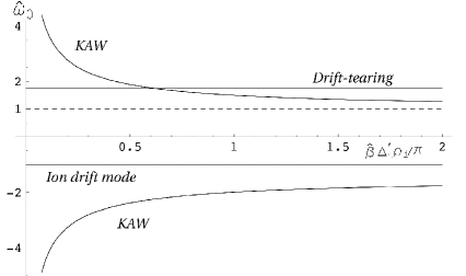
Figure 1: The solutions of the dispersion equation (34) for the drift-tearing mode and two KAWs as a function of $\Delta^{\prime}\rho_{i}\hat{\beta}/\pi.$ There is also an ion drift mode. The drift-tearing mode and the KAW propagating in the electron direction are strongly coupled in the vicinity of $\Delta^{\prime}\rho_{i}\hat{\beta}=(\Delta^{\prime}\rho_{i}\hat{\beta})_{c}$ given in Eq. (52).

Including the $\delta_{0}/\rho_{i}$ correction to Eq. (34), we find that these two KAWs are stable. The lowest order drift-tearing and KAW mode frequencies as functions of $\Delta^{\prime}\rho_{i}\hat{\beta}$ are shown schematically in Fig. 1. At large values of $\Delta^{\prime},$ a further solution of $C(\hat{\omega})=0$ is associated with the dissipative internal kink mode discussed in Section VII, while negative values of $\Delta^{\prime}$ give rise to the FLR modified ideal internal kink mode analysed in Ref. (Pegoraro and Schep, 1981).

However we note that at small $\hat{\beta}$ when $\delta_{0}/\rho_{i}\sim\hat{\beta}^{2},$ but $\Delta^{\prime}\rho_{i}\hat{\beta}\sim\mathcal{O}(1),$ which introduces an interaction between the drift-tearing mode and the KAWs, all four branches become coupled and Eq. (34) no longer has a natural expansion parameter.

III.2 The drift-tearing mode

Returning to the drift-tearing mode and assuming $\Delta^{\prime}\rho_{i}\hat{\beta}\ll 1$ so that we have an uncoupled mode, the lowest order solution, $D(\hat{\omega})=0,$ is given by

$$\left(1-\frac{1+1.71\eta_{e}}{\hat{\omega}}\right)\left(\frac{1+\tau}{\tau+\hat{\omega}^{-1}}\right)^{1/2}+1.45\left(1-\frac{1}{\hat{\omega}}\right)=0.$$ (39)

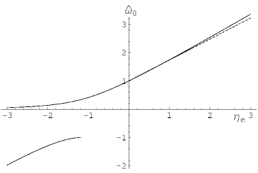
Figure 2: The drift-tearing mode frequency [the solution of Eq. (39)] as a function of $\eta_{e}$ for $\tau=1.$ For negative $\eta_{e}<-1.17$ a second solution exists. Also shown as a dotted line is the fit (40).

The solution of Eq. (39) is shown in Fig. 2; for $\eta_{e}>0$ (and $\tau=1$), a good fit to the solution is given by

$$\hat{\omega}=\hat{\omega}_{0}\approx 1+0.74\eta_{e}.$$ (40)

Figure 2 also shows a second solution for negative $\eta_{e},$ i.e. reversed density gradients or hollow temperature profiles; in fact it exists for $\eta_{e}<-(1+\tau^{-1})/1.71,$ i.e. $\eta_{e}<-1.17$ for $\tau=1,$ and for larger negative $\eta_{e}$ it can also be fitted by the form (40). Thus, in the limit of a flat density profile, one does obtain the same frequency, irrespective of the sign of $\eta_{e}.$ The growth rate follows from next order in $\delta_{0}/\rho_{i}:$

$$\hat{\gamma}\equiv\frac{\gamma}{\omega_{*e}}\sim\frac{\delta_{0}\hat{\omega}_{0}^{1/2}}{\pi\hat{\beta}}\left(\Delta^{\prime}-\Delta_{crit}^{\prime}\right),$$ (41)

where $\Delta_{crit}^{\prime}$ is the critical $\Delta^{\prime}$ for instability

$$\Delta_{crit}^{\prime}=\frac{\sqrt{\pi}\hat{\beta}}{\rho_{i}}\frac{1+\hat{\omega}_{0}\tau}{\hat{\omega}_{0}^{2}(1+\tau)^{2}}\left(\hat{\omega}_{0}\tau+1-\frac{\eta_{i}}{2}\right)(\hat{\omega}_{0}-1)^{2}\ln\left(e^{-\frac{\pi}{4}}\frac{\rho_{i}}{\delta_{0}\hat{\omega}_{0}^{1/2}}\right)-\frac{\pi\hat{\beta}}{\rho_{i}}(\hat{\omega}_{0}-1)\bar{I},$$ (42)

provided $\eta_{i}/2<\hat{\omega}_{0}\tau+1,$ where we note that expression (40) implies the factor $(\hat{\omega}_{0}-1)^{2}\propto\eta_{e}^{2}.$ This result closely resembles that obtained in Ref. (Cowley et al., 1986). The integral $\bar{I}[\hat{\omega}_{0}(\eta_{e}),\eta_{i},\tau],$ which is negative, scales approximately as $\bar{I}\approx\eta_{e}^{1/2},$ so the stabilising effect of this term resembles the diamagnetic stabilisation found in Ref. (Drake et al., 1983):

$$\Delta_{crit}^{\prime dia}=\frac{\pi\hat{\beta}}{\rho_{i}}(\hat{\omega}_{0}-1)\left|\bar{I}\right|$$ (43)

as can be seen by taking the $\tau\rightarrow\infty$ limit of Eq. (43), noting that $\bar{I}\sim\tau^{-1/2}$ in this situation.

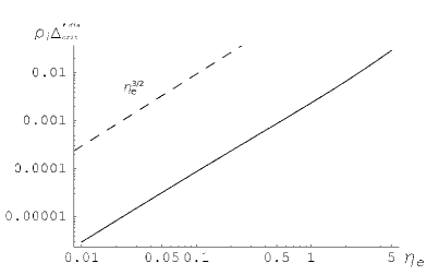
Figure 3: The scaling of the quantity $\Delta_{crit}^{\prime dia}$ in Eq. (43)

The quantity $\Delta_{crit}^{\prime dia}$ is shown as a function of $\eta_{e}$ in Fig. 3. The two different effects are shown in Fig. 4,

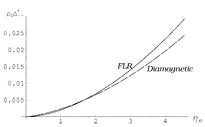
Figure 4: The diamagnetic and ion-kinetic contributions to the critical $\Delta^{\prime}$ [given in Eq. (43) and (44), respectively] as a function of the electron temperature gradients $\eta_{e}.$ Here $\hat{\beta}=10^{-3},$ $\delta_{0}/\rho_{i}=10^{-3},$ $\tau=1,$ $\eta_{i}=0.$

where

$$\Delta^{\prime\,FLR}_{crit}=\frac{\sqrt{\pi}\hat{\beta}}{\rho_{i}}\frac{1+\hat{\omega}_{0}\tau}{\hat{\omega}_{0}^{2}(1+\tau)^{2}}\left(\hat{\omega}_{0}\tau+1-\frac{\eta_{i}}{2}\right)(\hat{\omega}_{0}-1)^{2}\ln\left(e^{-\frac{\pi}{4}}\frac{\rho_{i}}{\delta_{0}\hat{\omega}_{0}^{1/2}}\right).$$ (44)

It should also be noted that, in principle, a large enough ion temperature gradient ($\eta_{i}/2>\hat{\omega}_{0}\tau+1$) can give a negative critical delta prime, however this requires values of $\eta_{i}$ that are probably only physically relevant in the flat density limit.

When $\eta_{e}<0$ we have seen there are solutions of Eq. (39) with $\hat{\omega}<1,$ in which case the integrand over $k$ in the integral $\bar{I}(\hat{\omega})$ has a pole at $k=k_{0},$ where $G(k_{0})=0.$ This zero in $G(k)$ corresponds to a resonance with an electrostatic drift wave of wave-number $k.$ The integral $\bar{I}(\hat{\omega})$ then has an imaginary contribution: by considering $\hat{\omega}$ to have a small imaginary part, we find the integral along real $k$ must pass above the pole at $k=k_{0}$ to ensure causality. This contribution provides a stabilising effect that increases the value of $\Delta_{crit}^{\prime}$ in Eq. (42) via damping on the electrostatic electron drift wave.

III.3 The kinetic Alfvén wave.

According to Eq. (41), as the tearing parameter $\Delta^{\prime}\rho_{i}/(\pi\hat{\beta})$ is increased beyond its marginal stability value (42), the drift-tearing mode becomes increasingly unstable. However, when $\Delta^{\prime}\rho_{i}\hat{\beta}\sim\mathcal{O}(1)$ the approximation $C(\hat{\omega}_{0})\approx 1$ fails; the dispersion relation can then be written in the form

$$e^{-i\frac{\pi}{4}}\frac{\delta_{0}}{\rho_{i}\hat{\beta}^{2}}A(\hat{\omega})\frac{\Delta^{\prime}\rho_{i}\hat{\beta}}{\pi}+\hat{\omega}\sqrt{1+\hat{\omega}\tau}\left[1-\frac{\Delta^{\prime}\rho_{i}\hat{\beta}}{\pi}\hat{\omega}(\hat{\omega}-1)I(\hat{\omega})\right]D(\hat{\omega})=0.$$ (45)

At the drift-tearing frequency, $\hat{\omega}_{0}\approx 1+0.74\eta_{e},$ the ion integral $\bar{I}$ is real and positive so the KAW propagating in the electron direction becomes strongly coupled to the drift-tearing branch when $\Delta^{\prime}\rho_{i}\hat{\beta}\sim\mathcal{O}(1).$ At yet higher values of this parameter the modes again decouple. We shall show below that the KAW propagating in the electron drift direction connects with the tearing mode having the frequency $\hat{\omega}_{0}.$ Because $C(\hat{\omega}_{0})$ has now changed sign, the branch with $\omega=\hat{\omega}_{0}$ has become stable. On the other hand the drift-tearing mode couples to the KAW given by the solution of $C(\hat{\omega}_{0})=0.$ Since one can show that, near $\hat{\omega}=1,$

$$I(\hat{\omega}_{0})\approx\frac{\pi}{2}\sqrt{\frac{(1+\tau+\eta_{i})/2}{\hat{\omega}-1}},$$ (46)

this branch has an unstable solution with

$$\hat{\omega}=1+\frac{2}{1+\tau+\eta_{i}}\left(\frac{2}{\Delta^{\prime}\rho_{i}\hat{\beta}}\right)^{2}-\frac{8\sqrt{2}\sqrt{d_{0}+2\sqrt{d_{1}}-1.71\eta_{e}/(1+\tau)}}{1.71\eta_{e}(1+\tau+\eta_{i})}\frac{1}{\hat{\beta}^{3}\Delta^{\prime}\rho_{i}}\frac{\delta_{0}}{\rho_{i}},$$ (47)

and a growth rate

$$\begin{split}&\hat{\gamma}=\frac{16}{\sqrt{2}\pi}\frac{\delta_{0}}{\rho_{i}}\frac{\sqrt{d_{0}+2\sqrt{d_{1}}-1.71\eta_{e}/(1+\tau)}}{\hat{\beta}^{3}\Delta^{\prime}\rho_{i}1.71\eta_{e}(1+\tau+\eta_{i})}\times\\ &\left[1-\frac{1}{\sqrt{2}\pi}\frac{\delta_{0}}{\rho_{i}}\frac{\Delta^{\prime}\rho_{i}}{\hat{\beta}}\frac{\sqrt{d_{0}+2\sqrt{d_{1}}-1.71\eta_{e}/(1+\tau)}}{1.71\eta_{e}}\right].\end{split}$$ (48)

Thus, as $\hat{\beta}$ increases, $\hat{\omega}\rightarrow 1$ and the growth rate decreases to zero. In fact, at very high values of $\Delta^{\prime}\rho_{i}$ the mode becomes stable. The condition for this is

$$\Delta^{\prime}\rho_{i}>2.42\pi\frac{\rho_{i}}{\delta_{0}}\frac{\eta_{e}\hat{\beta}}{\sqrt{d_{0}+2\sqrt{d_{1}}-1.71\eta_{e}/(1+\tau)}}.$$ (49)

This stabilisation mechanism does not exist when $\hat{\beta}<{(\delta_{0}/\rho_{i})}^{1/2}$ since the perturbative solution of Eq.(45) fails for $\Delta^{\prime}\rho_{i}\hat{\beta}\sim\mathcal{O}(1).$ Numerical solution shows that the unstable drift-tearing mode persists as $\Delta^{\prime}\rho_{i}$ increases beyond the critical value given in criterion (42), eventually merging with the dissipative kink instability discussed later in Section VII when $\Delta^{\prime}\rho_{i}\gg 1.$

We also note that Eq. (48) implies stability when

$$d_{0}+2\sqrt{d_{1}}-1.71\eta_{e}/(1+\tau)=0,$$ (50)

corresponding to a critical $\eta_{e}.$ Hence, as $\hat{\omega}\rightarrow 1,$ the drift tearing mode is also stable if

$$\eta_{e}>4.68(1+\tau).$$ (51)

III.4 The coupled modes

To analyse how the two branches interact we examine the solution of the dispersion relation (45) in the vicinity of the cross-over point. At this point, $C(\hat{\omega})=D(\hat{\omega})=0,$ so that $\hat{\omega}$ is given by the solution of Eq. (39), i.e. $\hat{\omega}=\hat{\omega}_{0},$ and the critical value of the parameter $\Delta^{\prime}\rho_{i}\hat{\beta}$ is given by

$$(\Delta^{\prime}\rho_{i}\hat{\beta})_{c}=\frac{\pi}{\hat{\omega}_{0}(\hat{\omega}_{0}-1)I(\hat{\omega}_{0},\eta_{i},\tau)},$$ (52)

where the integral $I$ is real and positive for modes propagating in the electron direction. Here the two modes interact strongly. After introducting $\delta\hat{\omega}=\hat{\omega}-\hat{\omega}_{0}$ and $\delta(\Delta^{\prime}\rho_{i}\hat{\beta})=\Delta^{\prime}\rho_{i}\hat{\beta}-(\Delta^{\prime}\rho_{i}\hat{\beta})_{c},$ a perturbation theory yields

$$(\delta\hat{\omega})^{2}\left(\frac{\partial C}{\partial\hat{\omega}}\frac{\partial D}{\partial\hat{\omega}}\right)_{\hat{\omega}_{0}}-\delta\hat{\omega}\left(\frac{\partial D}{\partial\hat{\omega}}\right)_{\hat{\omega}_{0}}\frac{\delta(\Delta^{\prime}\rho_{i}\hat{\beta})}{(\Delta^{\prime}\rho_{i}\hat{\beta})_{c}}+e^{-i\frac{\pi}{4}}\frac{\delta_{0}}{\rho_{i}}\frac{A(\hat{\omega}_{0})B(\hat{\omega}_{0})}{\hat{\omega}_{0}\sqrt{1+\hat{\omega}_{0}\tau}}=0.$$ (53)

One can trace how the branches reconnect about this point using the solution of Eq. (53):

$$\begin{split}&\delta\hat{\omega}_{\pm}=\frac{1}{2(\partial C/\partial\hat{\omega})_{\hat{\omega}_{0}}}\frac{\delta(\Delta^{\prime}\rho_{i}\hat{\beta})}{(\Delta^{\prime}\rho_{i}\hat{\beta})_{c}}\pm\frac{1}{2(\partial C/\partial\hat{\omega})_{\hat{\omega}_{0}}}\times\\ &\sqrt{\left[\frac{\delta(\Delta^{\prime}\rho_{i}\hat{\beta})}{(\Delta^{\prime}\rho_{i}\hat{\beta})_{c}}\right]^{2}-4e^{-i\frac{\pi}{4}}\frac{\delta_{0}}{\rho_{i}}\frac{(\partial C/\partial\hat{\omega})_{\hat{\omega}_{0}}}{(\partial D/\partial\hat{\omega})_{\hat{\omega}_{0}}}\frac{A(\hat{\omega}_{0})B(\hat{\omega}_{0})}{\hat{\omega}_{0}\sqrt{1+\hat{\omega}_{0}\tau}}}.\end{split}$$ (54)

When

$$\left[\frac{\delta(\Delta^{\prime}\rho_{i}\hat{\beta})}{(\Delta^{\prime}\rho_{i}\hat{\beta})_{c}}\right]^{2}\gg\left|4e^{-i\frac{\pi}{4}}\frac{\delta_{0}}{\rho_{i}}\frac{(\partial C/\partial\hat{\omega})_{\hat{\omega}_{0}}}{(\partial D/\partial\hat{\omega})_{\hat{\omega}_{0}}}\frac{A(\hat{\omega}_{0})B(\hat{\omega}_{0})}{\hat{\omega}_{0}\sqrt{1+\hat{\omega}_{0}\tau}}\right|,$$ (55)

solutions (54) simplify to

$$\begin{split}&\delta\hat{\omega}_{\pm}=\frac{1}{2(\partial C/\partial\hat{\omega})_{\hat{\omega}_{0}}}\frac{\delta(\Delta^{\prime}\rho_{i}\hat{\beta})}{(\Delta^{\prime}\rho_{i}\hat{\beta})_{c}}\pm\left|\frac{1}{2(\partial C/\partial\hat{\omega})_{\hat{\omega}_{0}}}\frac{\delta(\Delta^{\prime}\rho_{i}\hat{\beta})}{(\Delta^{\prime}\rho_{i}\hat{\beta})_{c}}\right|\\ &\mp e^{-i\frac{\pi}{4}}\frac{\delta_{0}}{\rho_{i}}\frac{A(\hat{\omega}_{0})B(\hat{\omega}_{0})}{\hat{\omega}_{0}\sqrt{1+\hat{\omega}_{0}\tau}}\left[\frac{1}{2(\partial D/\partial\hat{\omega})_{\hat{\omega}_{0}}}\frac{\delta(\Delta^{\prime}\rho_{i}\hat{\beta})}{(\Delta^{\prime}\rho_{i}\hat{\beta})_{c}}\right]^{-1}\mbox{sign}\left[(\partial C/\partial\hat{\omega})_{\hat{\omega}_{0}}\right].\end{split}$$ (56)

Thus we see that for $\Delta^{\prime}\rho_{i}\hat{\beta}<(\Delta^{\prime}\rho_{i}\hat{\beta})_{c},$ $\delta\hat{\omega}_{+}$ connects to the stable KAW branch, while for $\Delta^{\prime}\rho_{i}\hat{\beta}>(\Delta^{\prime}\rho_{i}\hat{\beta})_{c}$ it connects to the stable drift-tearing mode, whereas $\delta\hat{\omega}_{-}$ connects to the unstable drift-tearing mode for $\Delta^{\prime}\rho_{i}\hat{\beta}<(\Delta^{\prime}\rho_{i}\hat{\beta})_{c}$ and to the unstable KAW for $\Delta^{\prime}\rho_{i}\hat{\beta}>(\Delta^{\prime}\rho_{i}\hat{\beta})_{c}.$ This is shown in Fig. 5,

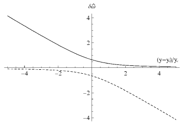
Figure 5: The variation of the real frequencies of the two modes with $\Delta^{\prime}\rho_{i}\hat{\beta},$ for fixed $\hat{\beta}=0.2$ and $\delta_{0}/\rho_{i}=0.1,$ in the vicinity of the cross-over point, $y\equiv\Delta^{\prime}\rho_{i}\hat{\beta}=(\Delta^{\prime}\rho_{i}\hat{\beta})_{c}\equiv y_{c}$ and $\hat{\omega}=\hat{\omega}_{0},$ showing how the KAW converts to the drift-tearing mode and vice versa. These results are for a typical case: $\eta_{e}=\eta_{i}=\tau=1.$

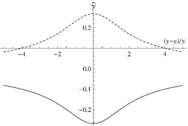
Figure 6: The equivalent variation of the growth/damping rates of the two modes in Fig. 5, showing how they peak at the cross-over point. These results are for $\eta_{e}=\eta_{i}=\tau=1.$

where we plot $\delta\hat{\omega}_{\pm}$ in the vicinity of the cross-over, by varying the parameter $\Delta^{\prime}\rho_{i}\hat{\beta}$ at constant $\hat{\beta}=0.2,$ for $\delta_{0}/\rho_{i}=0.1,$ and $\eta_{e}=\eta_{i}=\tau=1.$ [the quantities in Eq. (56) are very insensitive to these latter three parameters]. Very close to $\Delta^{\prime}\rho_{i}\hat{\beta}=(\Delta^{\prime}\rho_{i}\hat{\beta})_{c}$ the unstable branch has a larger growth rate than is given by Eq. (48), namely

$$\hat{\gamma}\sim\sqrt{\frac{\delta_{0}}{\rho_{i}}}.$$ (57)

In Fig. 6 we show the dependence of the growth (or damping) rates of the two modes for the same parameters as in Fig. 5.

IV The limit $\hat{\beta}\gg 1$

The analysis in the previous section was limited to the case $\hat{\beta}\ll 1;$ in this Section we explore the opposite case: $\hat{\beta}\gg 1.$ We anticipate that the “intermediate eigenvalue” $\mu$ will be finite, so that at high $\hat{\beta}$ we will have $\hat{\omega}-1\sim\mathcal{O}(\hat{\beta}^{-1}),$ as in Ref. (Drake et al., 1983). However, we have also seen in the low $\hat{\beta}$ theory of Section III that $\hat{\omega}\rightarrow 1$ when $\Delta^{\prime}\rho_{i}\hat{\beta}\gg 1.$ In Section V we will consider the fact that we can also have $\hat{\omega}-1\sim\varepsilon\ll 1$ at finite $\hat{\beta}$ to provide a bridge between the high and low $\hat{\beta}$ limits.

If $\hat{\omega}-1\sim\mathcal{O}(\hat{\beta}^{-1}),$ then $\sigma/d_{1}F(k)\ll 1$ in Eq. (8) for region $1,$ unless $k\ll 1,$ in which case $F(k)\propto k^{2}.$Thus for finite $k$ [not just for $k\gg 1$, as in Eq. (9)] the solution of Eq. (8) is

$$\hat{J}(k)=\hat{a}_{+}k^{1/2+\mu}+\hat{a}_{-}k^{1/2-\mu}.$$ (58)

For $k\ll 1,$ however, Eq. (8) takes the form

$$\frac{d}{dk}\left[\frac{2(1-\hat{\omega}^{-1})+(1+\eta_{i}+\tau)k^{2}}{(1+\eta_{i}+\tau)k^{2}}\right]\frac{d\hat{J}}{dk}+\left(\frac{1}{4}-\mu^{2}\right)\frac{\hat{J}}{k^{2}}=0.$$ (59)

This has a solution

$$\begin{split}&\hat{J}(k)=a_{1}\,{}_{2}F_{1}\left(-\frac{1}{4}+\frac{\mu}{2},-\frac{1}{4}-\frac{\mu}{2};-\frac{1}{2};y\right)\\ &+a_{2}y^{3/2}\,_{2}F_{1}\left(\frac{5}{4}+\frac{\mu}{2},\frac{5}{4}-\frac{\mu}{2};\frac{5}{2};y\right),\end{split}$$ (60)

where ${}_{2}F_{1}$ is the hypergeometric function (Abramowitz and Stegun, 1972a),

$$y=-\kappa^{2}k^{2},\,\,\,\,\,\,\,\kappa^{2}=\frac{1+\eta_{i}+\tau}{2(1-\hat{\omega}^{-1})},$$ (61)

and $a_{1}$ and $a_{2}$ are two constants to be determined by matching solution (60) to the ideal MHD boundary condition (11) for $k\ll 1.$ This matching condition yields

$$\frac{a_{2}}{a_{1}}=i\frac{\pi}{3\kappa}\frac{\hat{\beta}(1+\tau+\eta_{i})}{\Delta^{\prime}\rho_{i}}.$$ (62)

The large $k$ behaviour of solution (60) is given by

$$\begin{split}&\hat{J}(k)\sim y^{1/4-\mu/2}\left[a_{1}\frac{\Gamma(-1/2)\Gamma(-\mu)}{\Gamma^{2}(-1/4-\mu/2)}-ia_{2}\frac{\Gamma(5/2)\Gamma(-\mu)}{\Gamma^{2}(5/4-\mu/2)}\right]\\ &+y^{1/4+\mu/2}\left[a_{1}\frac{\Gamma(-1/2)\Gamma(\mu)}{\Gamma^{2}(-1/4+\mu/2)}-ia_{2}\frac{\Gamma(5/2)\Gamma(\mu)}{\Gamma^{2}(5/4+\mu/2)}\right]\,\,\,\mbox{for}\,\,\,k\rightarrow\infty,\end{split}$$ (63)

where $\Gamma$ is the Euler Gamma function (Abramowitz and Stegun, 1972b). Thus, the asymptotic form given by Eq. (63) implies the quantites $\hat{a}_{\pm}$ in Eq. (9) are related by

$$\frac{\hat{a}_{-}}{\hat{a}_{+}}=\kappa^{-2\mu}\frac{\Gamma(-\mu)}{\Gamma(\mu)}\frac{\frac{1}{\Gamma^{2}(-\mu/2-1/4)}+i\frac{3}{8}\frac{a_{2}}{a_{1}}\frac{1}{\Gamma^{2}(-\mu/2+5/4)}}{\frac{1}{\Gamma^{2}(\mu/2-1/4)}+i\frac{3}{8}\frac{a_{2}}{a_{1}}\frac{1}{\Gamma^{2}(\mu/2+5/4)}}.$$ (64)

In region $2$ we follow the treatment of Ref. (Drake et al., 1983) to solve Eq. (17), obtaining a solution that is small at $s=0:$

$$J(s)=\frac{\sigma_{0}+\sigma_{1}s^{2}}{1+\bar{d}_{0}s^{2}+\bar{d}_{1}s^{4}}\sqrt{\frac{s}{s_{t}}}K_{\mu}\left(\frac{s_{t}}{s}\right),$$ (65)

where $K_{\mu}$ is a modified Bessel function (Abramowitz and Stegun, 1972c) and $s_{t}^{2}=1.71\eta_{e}\hat{\beta}/d_{1}.$ For large $s$ this has the form

$$J(s)\sim\frac{1}{\Gamma(1-\mu)}\left(\frac{2s}{s_{t}}\right)^{-3/2+\mu}-\frac{1}{\Gamma(1+\mu)}\left(\frac{2s}{s_{t}}\right)^{-3/2-\mu},\,\,\,s\rightarrow\infty.$$ (66)

Calculating the Fourier transform of expression (66) we obtain

$$\frac{b_{-}}{b_{+}}=-\left(\frac{s_{t}}{2}\right)^{2\mu}\frac{\Gamma(1-\mu)}{\Gamma(1+\mu)}.$$ (67)

Thus, with the aid of Eq. (20), we have

$$\frac{\hat{c}_{-}}{\hat{c}_{+}}=-\left(\frac{2}{s_{t}}\right)^{2\mu}\frac{\Gamma(\mu-1/2)\Gamma(1+\mu)}{\Gamma(-\mu-1/2)\Gamma(1-\mu)}\tan\left[\frac{\pi}{2}\left(\frac{1}{2}+\mu\right)\right].$$ (68)

Finally, matching region $1$ and region $2$ solutions, we obtain the dispersion relation

$$e^{i\frac{\pi}{2}\mu}R^{\mu}=\frac{(\mu+1/2)\Gamma^{2}(-\mu)}{(-\mu+1/2)\Gamma^{2}(\mu)}\left\{\frac{\mathcal{D}-\cot\left[\pi\left(\frac{1}{4}+\frac{\mu}{2}\right)\right]}{\mathcal{D}-\cot\left[\pi\left(\frac{1}{4}-\frac{\mu}{2}\right)\right]}\right\},$$ (69)

where

$$R=\frac{8d_{1}}{1.71\eta_{e}}\frac{\rho_{i}^{2}}{\delta_{0}^{2}}\frac{1+\tau+\eta_{i}}{1/4-\mu^{2}},$$ (70)

and

$$\mathcal{D}=\frac{\sqrt{2}}{\pi}\Delta^{\prime}\rho_{i}\frac{(1+\tau+\eta_{i})^{1/2}}{(\hat{\omega}-1)^{1/2}}\frac{\Gamma(5/4-\mu/2)\Gamma(5/4+\mu/2)}{\Gamma(3/4-\mu/2)\Gamma(3/4+\mu/2)}.$$ (71)

Introducing the collisionality parameter $C$ of Ref. (Drake et al., 1983),

$$C=0.51\frac{\nu_{e}}{\omega_{*e}}\frac{m_{e}}{m_{i}}\frac{L_{s}^{2}}{L_{n}^{2}}=2.04\frac{\delta_{0}^{2}}{\tau\rho_{i}^{2}},$$ (72)

equation (69) can be recognised as essentially identical to their semi-collisional, high $\hat{\beta},$ cold ion result, generalised to finite $T_{i}/T_{e}$ and $\eta_{i}.$ While surprising at first sight, we see that the solution (60) of Eq. (8) only utilised the low $k$ expansion of $F(k),$ corresponding to a small ion Larmor radius approximation, although the solution remained valid for finite $k.$ Furthermore, this is the solution that we would have obtained using a Padé approximation to $F(k),$ as in Ref. (Pegoraro et al., 1989); however, here it is exact for $\hat{\beta}\gg 1.$ As is evident from our low $\hat{\beta}$ result, this approximation fails to capture the “$1/k$ tail” of $F(k)$ at high $k$ in Eq. (5) that is essential to the result of Ref. (Cowley et al., 1986).

As shown in Ref. (Drake et al., 1983), the dispersion relation (69) predicts stability for all values of $\Delta^{\prime}.$ An analysis at large $\Delta^{\prime}$ shows the damping rate becomes small

$$\hat{\gamma}\sim-1/(R^{1/2}\Delta^{\prime}\rho_{i}).$$ (73)

The result (48), representing the KAW branch with $\hat{\omega}\approx 1$ at lower $\hat{\beta},$ also has a growth rate that tends to zero as $(\Delta^{\prime}\rho_{i}\hat{\beta}^{3})^{-1}.$ In the next Section we present a model that demonstrates how the transition to stability occurs at finite $\hat{\beta}.$

V Transition to Stability at Finite $\hat{\beta}$

As we have seen, the KAW branch has a frequency approaching $\hat{\omega}\approx 1$ as $\hat{\beta}$ increases, as also does the high $\hat{\beta}$ theory, and we exploit this property to explore the effect of finite $\hat{\beta},$ i.e. $\hat{\beta}\sim\mathcal{O}(1).$ For finite $s,$ Eq. (17) takes the form

$$\frac{d^{2}}{ds^{2}}\left\{1+[d_{0}-1.71\eta_{e}/(1+\tau)]s^{2}+d_{1}s^{4}\right\}J-1.71\eta_{e}\hat{\beta}J=0.$$ (74)

If we consider the special case

$$d_{0}-1.71\eta_{e}/(1+\tau)=2\sqrt{d_{1}},$$ (75)

corresponding to $\eta_{e}=2.53$ for $\tau=1,$ and introduce $u=d_{1}^{1/4}s,$ then we can write Eq. (74) as

$$\frac{d^{2}}{du^{2}}\left(1+u^{2}\right)^{2}J-\lambda^{2}J=0,\,\,\,\,\lambda^{2}=\frac{1.71\eta_{e}\hat{\beta}}{\sqrt{d_{1}}}=\sqrt{d_{1}}s_{t}^{2}.$$ (76)

The solution, even at $s=0,$ is

$$J(s)=\left(1+u^{2}\right)^{-3/2}\cos\left(\sqrt{1-\lambda^{2}}\arctan u\right),$$ (77)

which has the large $s$ asymptotic behaviour

$$J(s)\sim s^{-3}-\frac{\sqrt{1-\lambda^{2}}}{d_{1}^{1/4}}\tanh\left(\frac{\pi}{2}\sqrt{\lambda^{2}-1}\right)s^{-4},\,\,\,s\gg 1.$$ (78)

When $s$ is such that $(\hat{\omega}-1)s^{2}\sim 1,$ the solution for $J(s)$ is obtained in terms of modified Bessel functions, as in Eq. (65), except that now we no longer impose the vanishing boundary condition for small $s,$ but match to the form (78) instead. Thus we obtain

$$J(s)\propto\frac{\lambda^{2}/\hat{\beta}\sqrt{d_{1}}-(\hat{\omega}-1)s^{2}}{s^{7/2}}\left[\tilde{a}_{1}K_{\mu}\left(\frac{s_{t}}{s}\right)+\tilde{a}_{2}I_{\mu}\left(\frac{s_{t}}{s}\right)\right],$$ (79)

where $\tilde{a}_{1}$and $\tilde{a}_{2}$ are constants and we note $\mu^{2}=1/4-(\hat{\omega}-1)\hat{\beta}\approx 1/4.$ Matching the small argument limit of this solution to the form (78), with $\mu\approx 1/2$ and $\hat{\omega}\approx 1,$ yields the relationship between $\tilde{a}_{1}$and $\tilde{a}_{2}:$

$$\frac{\tilde{a}_{2}}{\tilde{a}_{1}}=\frac{\pi}{2}\left[1-\frac{\sqrt{\lambda^{2}-1}}{\lambda}\tanh\left(\frac{\pi}{2}\sqrt{\lambda^{2}-1}\right)\right].$$ (80)

At high $\hat{\beta},$ i.e. high $\lambda,$ we see that $\tilde{a}_{2}/\tilde{a}_{1}\rightarrow 0,$ and we recover the results in the previous Section.

When $(\hat{\omega}-1)s^{2}\gg 1,$ the solution (79) has the correct form to match to the solution (63) in region $1.$ As a result we obtain a dispersion relation

$$e^{i\frac{\pi}{2}\mu}R^{\mu}=\Lambda\left(\mu,\lambda\right)\frac{(\mu+1/2)\Gamma^{2}(-\mu)}{(-\mu+1/2)\Gamma^{2}(\mu)}\left\{\frac{\mathcal{D}-\cot\left[\frac{\pi}{2}\left(\frac{1}{2}+\mu\right)\right]}{\mathcal{D}-\cot\left[\frac{\pi}{2}\left(\frac{1}{2}-\mu\right)\right]}\right\},$$ (81)

which only differs from expression (69) by the key “shielding factor” $\Lambda\left(\mu,\lambda\right):$

$$\Lambda\left(\mu,\lambda\right)=1-\sin(\pi\mu)\left[1-\frac{\sqrt{\lambda^{2}-1}}{\lambda}\tanh\left(\frac{\pi}{2}\sqrt{\lambda^{2}-1}\right)\right].$$ (82)

For consistency we need to consider $\Lambda\left(\mu,\lambda\right)$ in the limit $\mu\rightarrow 1/2.$ We note that then $\Lambda\approx 1$ for $\lambda\gg 1,$ $\Lambda=0$ for $\lambda=1$ and $\Lambda\approx-4/(\pi\lambda^{3})$ for $\lambda\ll 1.$

Recalling $R\gg 1,$ we observe that Eq. (81) has a solution with $\mu\approx 1/2,$ as required if our ordering is to be consistent. This solution is obtained by balancing the large left-hand-side of Eq. (81) by approaching the zero of the denominator on its right-hand-side. Writing $\mu\approx 1/2-\hat{\beta}\delta\hat{\omega},$ we find

$$\hat{\omega}\approx 1+\frac{2}{1+\tau+\eta_{i}}\left(\frac{2}{\hat{\beta}\Delta^{\prime}\rho_{i}}\right)^{2}+\frac{2\sqrt{2}\Lambda}{\hat{\beta}^{3/2}\Delta^{\prime}\rho_{i}(1+\tau+\eta_{i})}\left(\frac{1.71}{d_{1}}\eta_{e}\right)^{1/2}\frac{\delta_{0}}{\rho_{i}},$$ (83)

$$\hat{\gamma}\approx-4\sqrt{2}\Lambda\frac{\delta_{0}}{\rho_{i}}\left(\frac{1.71}{d_{1}}\frac{\eta_{e}}{\hat{\beta}}\right)^{1/2}\frac{1}{\hat{\beta}\Delta^{\prime}\rho_{i}(1+\tau+\eta_{i})}\left(1+\Lambda\frac{\Delta^{\prime}\rho_{i}\hat{\beta}^{1/2}}{2\sqrt{2}}\frac{\delta_{0}}{\rho_{i}}\sqrt{\frac{1.71}{d_{1}}\eta_{e}\hat{\beta}}\right),$$ (84)

which shows that we require $\hat{\beta}\Delta^{\prime}\rho_{i}\gg 1$ for consistency. In the small $\hat{\beta}$ limit the growth rate reduces to

$$\hat{\gamma}\approx\frac{32}{\pi\sqrt{2}}\frac{\delta_{0}}{\rho_{i}}\frac{d_{1}^{1/4}}{1.71\eta_{e}}\frac{1}{\hat{\beta}^{3}\Delta^{\prime}\rho_{i}(1+\tau+\eta_{i})}\left(1-\frac{\sqrt{2}d_{1}^{1/4}}{1.71}\frac{\Delta^{\prime}\rho_{i}}{\eta_{e}\hat{\beta}}\frac{\delta_{0}}{\rho_{i}}\right).$$ (85)

Taking account of the condition (75) on $\eta_{e},$ we see that this coincides with the low $\hat{\beta}$ result (48) of the KAW; similarly, the frequency $\hat{\omega}$ reduces to the result (47).

Equation (84) implies stability if $\Lambda>0.$ This stability boundary corresponds to $\lambda=1,$ so that there is stability for values of $\hat{\beta}$ satisfying

$$\hat{\beta}>\hat{\beta}_{c}\equiv\frac{\sqrt{d_{1}}}{1.71\eta_{e}}=0.34,$$ (86)

for $\tau=1.$ Thus the model correctly predicts stability at high $\hat{\beta}$ as found in Section IV. If $\Lambda<0$ then there is still stability if $\Delta^{\prime}$ is sufficiently large:

$$\Delta^{\prime}\delta_{0}\sqrt{\frac{1.71}{d_{1}}\hat{\beta}\eta_{e}}>-\frac{1}{\Lambda}.$$ (87)

For $\hat{\beta}\rightarrow\hat{\beta}_{c},$ one finds stability if

$$\Delta^{\prime}\delta_{0}>\frac{\pi}{4\sqrt{2}}\sqrt{\frac{1.71\eta_{e}}{d_{1}}}\frac{1}{\hat{\beta}_{c}-\hat{\beta}}.$$ (88)

As $\hat{\beta}$ reduces, $-\Lambda$ increases and the necessary value of $\Delta^{\prime}$ for stability decreases. At low $\hat{\beta}$ the result is consistent with the stability condition (49). We note that a similar analysis can be performed for another special case:

$$d_{0}-1.71\eta_{e}/(1+\tau)=-2\sqrt{d_{1}}.$$ (89)

Now, however, we find the analogue of the screening factor $\Lambda$ is always positive so the mode is always stable. Condition (89), which guarantees stability at finite $\hat{\beta},$ coincides with condition (75), the stability condition at low $\hat{\beta},$ so we have a consistent picture.

Although our model equation is strictly valid for a specific, though reasonable, value of $\eta_{e},$ it captures in a clear way the onset of screening by plasma gradients that stabilises modes in high $\hat{\beta}$ plasma.

VI Tearing Mode stability Diagram

In this section we draw together results from previous sections concerning the stability of the drift-tearing and kinetic Alfvén waves, summarising them in Fig. 7, a diagram in the space of $\hat{\beta}$ and $\Delta^{\prime}\rho_{i}$ which delineates stable and unstable regions and regions of validity of these results.

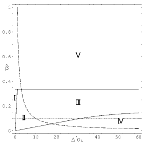
Figure 7: Stability diagram for the drift-tearing/kinetic Alfvén mode in terms of $\Delta^{\prime}\rho_{i}$ and $\hat{\beta}.$ Regions I, IV and V are stable, Regions II and III unstable. The finite $\hat{\beta}$ analysis is not valid in the region below the hyperbola $\hat{\beta}\Delta^{\prime}\rho_{i}=1$ (dashed line); the low $\hat{\beta}$ theory fails below the dotted line $\hat{\beta}=(\delta_{0}/\rho_{i})^{1/2}$ when $\hat{\beta}\Delta^{\prime}\rho_{i}\sim\mathcal{O}(1).$ Here $\delta_{0}/\rho_{i}=10^{-2}.$

The low $\hat{\beta}$ theory of Section III.2, valid for $\hat{\beta}\ll 1,$ shows that the drift-tearing mode is stable in Region I, becoming unstable in Region II when $\Delta^{\prime}\rho_{i}$ exceeds the critical value given in criterion (42). When the approximate boundary $\Delta^{\prime}\rho_{i}\hat{\beta}\sim\mathcal{O}(1)$ is exceeded as in Region III, the analysis in Section III.3 is valid and the kinetic Alfvén wave becomes the unstable branch; this remains unstable until the criterion (49) is satisfied and one enters the stable Region IV. Above a critical value of $\hat{\beta}=\hat{\beta}_{c}\sim\mathcal{O}(1),$ given precisely by condition (86) in Section V for the special case of $\eta_{e}$ specified in Eq.(75), the kinetic Alfvén wave is stable, as represented by Region V. This stability region extends to high $\hat{\beta}$ as shown in Section IV. The boundary between Regions IV and III asymptotes to the critical value of $\hat{\beta}$ following the scaling $\Delta^{\prime}\propto(\hat{\beta}_{c}-\hat{\beta})^{-1}.$ The low $\hat{\beta}$ results discussed above are limited by the condition $\hat{\beta}>{(\delta_{0}/\rho_{i})}^{1/2}$ (dotted line in Fig. 7) when $\Delta^{\prime}\rho_{i}\hat{\beta}\sim\mathcal{O}(1).$ Below the dotted line, there is still an instability when $\Delta^{\prime}\rho_{i}$ exceeds the critical value from the criterion (42), beyond which the growth rate continues to increase with $\Delta^{\prime}\rho_{i},$ eventually merging with the dissipative kink mode, discussed in the next Section, when $\Delta^{\prime}\rho_{i}\gg 1.$

VII The Internal Kink Mode

VII.1 Low $\hat{\beta}$ theory

In this Section we analyse the internal kink mode. When $\Delta^{\prime}<0$ we first follow Pegoraro et al. (Pegoraro et al., 1989) in introducing the growth rate of the ideal MHD internal kink mode: $\lambda_{H}=-\pi/\Delta^{\prime}r_{s},$ where $q(r_{s})=1.$ The solution of the branch $C(\hat{\omega})=0$ of the general dispersion relation (34) then reproduces the FLR modified internal kink mode dispersion relation obtained, and analysed numerically, in Ref. (Pegoraro et al., 1989). The small terms on the left-hand-side of Eq. (34) can be retained to obtain a correction to the ideal result. However, in the limit $\lambda_{H}\rightarrow 0$ these terms must be retained to obtain the dispersion relation for the dissipative internal kink mode which is associated with the $\hat{\omega}\approx 0$ branch of Eq. (36).

For small values of $|\hat{\omega}|$ and $\hat{\beta}\ll 1,$ we can approximate the terms in Eq. (34):

$$\begin{split}&A(\hat{\omega})=\sqrt{1+\tau}\sqrt{d_{0}-(1+1.71\eta_{e})}\equiv\sqrt{(1+\tau)d(\eta_{e})}\\ &B(\hat{\omega})=\frac{\Delta^{\prime}\rho_{i}}{\pi\hat{\beta}}\hat{\omega}\\ &C(\hat{\omega})=1+\frac{\Delta^{\prime}\rho_{i}}{\pi}\hat{\beta}\hat{\omega}I(\hat{\omega},\tau,\eta_{i})\\ &D(\hat{\omega})=-\sqrt{d_{1}},\end{split}$$ (90)

where now we require $\Delta^{\prime}\rho_{i}|\hat{\omega}|/(\pi\hat{\beta})\gg 1.$ Assuming $\hat{\omega}$ to be real and negative, i.e. in the ion direction, we can calculate the integrals analytically:

$$I(\hat{\omega},\eta_{i})=-\sqrt{\pi}I_{2}(\eta_{i},\tau)-\frac{\sqrt{\pi}}{1-\eta_{i}/2}\ln\left[\frac{1-\eta_{i}/2}{-\hat{\omega}(1+\tau)\sqrt{\pi}}\right],$$ (91)

where

$$I_{2}(\eta_{i},\tau)=\frac{1}{\sqrt{\pi}}\int_{0}^{\infty}\frac{dk}{k^{2}}\left[\frac{F_{0}}{G_{0}}-\frac{\sqrt{\pi}}{1-\eta_{i}/2}\frac{k^{2}}{(1+k)}\right].$$ (92)

The quantity $(1-\eta_{i}/2)I_{2}(\eta_{i},\tau)$ is plotted in Fig. 8 as a function of $\eta_{i}$ for $\tau=1.$

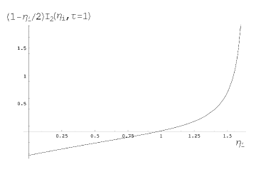
Figure 8: The function $(1-\eta_{i}/2)I_{2}$ appearing in Eq. (92) as a function of $\eta_{i}$ for $\tau=1$.

For consistency, the present analysis of Eq. (34) is limited to the situation where $\delta_{0}/\rho_{i}\hat{\beta}\ll 1$ to ensure $|\hat{\omega}|\ll 1.$

Substituting the result (90) into Eq. (45) and expressing $\Delta^{\prime}$ in terms of $\lambda_{H},$ we obtain a dispersion relation

$$\begin{split}&\hat{\omega}\left\{\ln\left[\frac{(1+\tau)\sqrt{\pi}}{1-\eta_{i}/2}\hat{\omega}\right]-i\pi-\left(1-\frac{\eta_{i}}{2}\right)I_{2}-\frac{1}{\sqrt{\pi}}\left(1-\frac{\eta_{i}}{2}\right)\frac{\lambda_{H}}{\rho_{i}}\frac{1}{\hat{\beta}\hat{\omega}}\right\}=\\ &\sqrt{\frac{1+\tau}{\pi d_{1}}d(\eta_{e})}\left(1-\frac{\eta_{i}}{2}\right)\frac{\delta_{0}}{\rho_{i}\hat{\beta}^{2}}e^{-i\frac{\pi}{4}},\end{split}$$ (93)

which is valid for $|\lambda_{H}/\rho_{i}|\ll 1.$ For the special case $\lambda_{H}=0$ this produces, as in Ref. (Jardin et al., 1993), an unstable mode rotating in the ion direction

$$\hat{\omega}=-\sqrt{d(\eta_{e})\frac{1+\tau}{2\pi d_{1}}}\left(1-\frac{\eta_{i}}{2}\right)\frac{1}{\ln(\rho_{i}\hat{\beta}^{2}/\delta_{0})}\frac{\delta_{0}}{\rho_{i}\hat{\beta}^{2}}e^{-i\frac{\pi}{4}},$$ (94)

where we have iterated on the $\ln(-\hat{\omega}^{-1})$ term, ignoring $\mathcal{O}(1)$ corrections. When $\delta_{0}/\rho_{i}\ll\hat{\beta}\left|\lambda_{H}\right|/\rho_{i}\ll\hat{\beta}^{2}$ we obtain a stable mode in the electron direction:

$$\hat{\omega}=\frac{1}{\sqrt{\pi}}\left(1-\frac{\eta_{i}}{2}\right)\frac{\left|\lambda_{H}\right|}{\rho_{i}\hat{\beta}\,\ln(\rho_{i}\hat{\beta}/\left|\lambda_{H}\right|)}\left[1-\frac{i\pi}{\ln(\rho_{i}\hat{\beta}/\left|\lambda_{H}\right|)}\right].$$ (95)

Thus there is a marginally stable value of $\lambda_{H},$ which can be found by equating real and imaginary parts, with $\hat{\omega}$ real, in Eq. (93), to yield

$$\lambda_{H}^{crit}=-\delta_{0}\frac{1}{\pi\hat{\beta}}\sqrt{d(\eta_{e})\frac{1+\tau}{2d_{1}}}\left\{\ln\left[\hat{\beta}^{2}\frac{\rho_{i}}{\delta_{0}}\frac{\pi}{(1+\tau)^{3/2}}\sqrt{\frac{2d_{1}}{d(\eta_{e})}}\right]+\pi+\left(1-\frac{\eta_{i}}{2}\right)I_{2}(\eta_{i})\right\}.$$ (96)

The condition that $|\hat{\omega}|$ remains small at these value of $\lambda_{H}$ requires

$$\hat{\beta}>\left(\frac{\delta_{0}}{\rho_{i}}\right)^{1/2}.$$ (97)

We note that the numerical solution at high $\Delta^{\prime}\rho_{i}$ in the region $\delta_{0}/\rho_{i}\gg\hat{\beta}^{2}$ described in Section III.3 can be followed through the boundary $\hat{\beta}\sim{(\delta_{0}/\rho_{i})}^{1/2}$ to merge with the result (94). We identify also a strong stabilising effect from $\eta_{e}:$ Eq. (90) implies the factor $d(\eta_{e})$ becomes negative, corresponding to stability, if

$$\eta_{e}>(d_{0}-1)/1.71\approx 2.38.$$ (98)

Using Eq. (72) we can express the results (94), (95) and (96) in terms of the collisionality parameter $C$ of Ref. (Drake et al., 1983).

VII.2 Finite $\hat{\beta}$ theory

Because the dissipative internal kink mode corresponds to $|\hat{\omega}|\ll 1$ we can seek a solution of Eqs. (8) and (17) based on an expansion in $\hat{\omega}$ at finite $\hat{\beta},$ rather that in $\hat{\beta}$ at finite $\hat{\omega},$ as in Section III. The details are presented in the Appendix but we note the essential points here. For the ions we can exploit the same expansion as in Eq. (22), but now based on $|\hat{\omega}|\ll 1;$ in this region of $k$, $F(k)$ and $G(k)$ take simpler forms. However, this expansion fails at large $k\sim\hat{\omega}^{-1}$ when the finite $\hat{\omega}$ correction to $G(k)$ becomes important. The ion response must be calculated in this intermediate region with $k\sim\hat{\omega}^{-1}$ before the solution can be matched to the electron region. The electron solution, i.e. the solution of Eq. (17) calculated in real space, also exploits the condition $|\hat{\omega}|\ll 1$ by considering two sub-regions. In the first of these we consider $s\sim\mathcal{O}(1)$ when we take advantage of the fact that the quadratic term in the demonimator of the conductivity in Eq. (15) can be ignored. In the second sub-region we take $s\sim|\hat{\omega}|^{-1/2}\gg 1$ which again simplifies the equation so that an analytic solution can be obtained. We match the solutions in the two sub-regions at intermediate values of $s$, deduce the power-like asymptotic form for $s\gg|\hat{\omega}|^{-1/2}$ and then use Eq. (20) to obtain the solution in $k-$space. Finally we match this electron region solution to the intermediate ion region solution to provide a dispersion relation for the dissipative internal kink mode. This relation is given by Eq. (136) in the Appendix, which we reproduce here:

$$\left[\frac{e^{-i\frac{5}{4}\pi}}{8\sqrt{\pi}\hat{\omega}}\frac{\delta_{0}}{\rho_{i}}\sqrt{\frac{d(\eta_{e})}{d_{1}}}\,\frac{1-\eta_{i}/2}{(1+\tau)^{3/2}}\right]^{2\mu_{1}}=\frac{1/2-\mu_{1}}{1/2+\mu_{1}}\frac{\Gamma^{2}(\mu_{1})}{\Gamma^{2}(-\mu_{1})}\frac{\Sigma(\hat{\omega})+i\frac{\hat{\beta}}{1+\tau}e^{i\pi\mu_{1}}}{\Sigma(\hat{\omega})+i\frac{\hat{\beta}}{1+\tau}e^{-i\pi\mu_{1}}}.$$ (99)

We recall that we can express $\delta_{0}/\rho_{i}$ in terms of the collisionality parameter $C,$ [note $\delta_{0}/(8\rho_{i})=0.088\tau^{1/2}C^{1/2}$]. Here $\Sigma$ is

$$\begin{split}&\Sigma(\hat{\omega})=-\frac{\cos[\pi\mu_{1}]}{\pi}\left\{1-\frac{1}{\sqrt{\pi}}\frac{1-\eta_{i}/2}{1+\tau}\frac{\lambda_{H}}{\rho_{i}}\frac{1}{\hat{\omega}}-\hat{\beta}\frac{1-\eta_{i}/2}{1+\tau}I_{2}\right.\\ &\left.+\frac{\hat{\beta}}{1+\tau}\left[\frac{3}{2}-k_{0}+\ln\left(\frac{\sqrt{\pi}(1+\tau)}{1-\eta_{i}/2}\hat{\omega}\right)\right]\right\},\end{split}$$ (100)

with $2\mu_{1}=\sqrt{1+4\hat{\beta}/(1+\tau)},$ $k_{0}=\psi(1)+\psi(3)-\psi(3/2-\mu_{1})-\psi(3/2+\mu_{1}),$ where $\psi$ is the digamma function (Abramowitz and Stegun, 1972b). We can solve this analytically in the low $\hat{\beta}$ limit. Assuming the logarithmic term in Eq. (100) dominates, we recover the result (93). However Eq. (99) allows us to explore the effect of finite $\hat{\beta}$ on the stability of the dissipative internal kink mode.

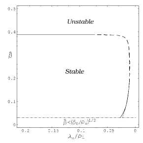
Figure 9: The boundary of marginal stability for the dissipative internal kink mode when |$\lambda_{H}/\rho_{i}|\ll 1.$ The complete line is from the numerical solution of the dispersion relation (99). The dashed line is the analytical boundary of Eq. (101), the dotted line is the low $\hat{\beta}$ analytical limit of Eq. (96). Here $\delta_{0}/\rho_{i}=10^{-3},$ $\eta_{e}=\tau=1,$ $\eta_{i}=0.$ In the region $\hat{\beta}<(\delta_{0}/\rho_{i})^{1/2},$ the finite $\hat{\beta}$ theory breaks down.

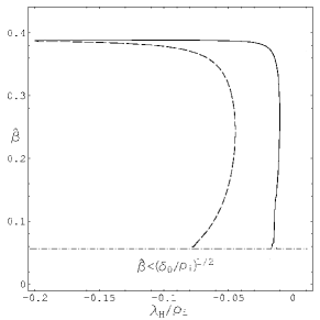
Figure 10: Boundary of the marginal stability region for the dissipative internal kink mode from the numerical solution of Eq. (99). Solid line: $\delta_{0}/\rho_{1}=10^{-3},$ dashed line: $\delta_{0}/\rho_{1}=10^{-2}.$

For low values of $\hat{\beta}/(1+\tau)$ there is a threshold value for $\left|\lambda_{H}\right|$ for the onset of the instability, as in Eq. (96), but this is lost as $\hat{\beta}/(1+\tau)$ increases beyond $0.194.$ It is again possible to calculate the marginal value of $\left|\lambda_{H}\right|$ by equating real and imaginary parts of Eq. (99) with real $\hat{\omega}$ (for a consistent solution we must take $\hat{\omega}=\exp(-2\pi i)\hat{\omega}_{1},$ with $\hat{\omega}_{1}$ real and positive):

$$\begin{split}&\lambda_{H}^{crit}=-\delta_{0}H(\mu_{1})\frac{\sqrt{1+\tau}}{8}\sqrt{\frac{d(\eta_{e})}{d_{1}}}\times\\ &\left\{\frac{\hat{\beta}}{1+\tau}\frac{\pi}{\cos(\pi\mu_{1})}\sqrt{\frac{\sin(\pi\mu_{1}/2)}{\sin(3\pi\mu_{1}/2)}}-1\right.\\ &\left.-\frac{\hat{\beta}}{1+\tau}\left[\frac{3}{2}-k_{0}-\left(1-\frac{\eta_{i}}{2}\right)I_{2}+\ln\left(\frac{\delta_{0}}{\rho_{i}}H(\mu_{1})\frac{\sqrt{1+\tau}}{8}\sqrt{\frac{d(\eta_{e})}{d_{1}}}\right)\right]\right\},\end{split}$$ (101)

while $\hat{\omega}$ is given by

$$\hat{\omega}=\frac{1}{8}\frac{\delta_{0}}{\rho_{i}}H(\mu_{1})\sqrt{\frac{d_{1}}{\pi d(\eta_{e})}}\frac{1-\eta_{i}/2}{(1+\tau)^{3/2}}.$$ (102)

Here

$$H(\mu_{1})=\left\{\frac{1/2+\mu_{1}}{1/2-\mu_{1}}\frac{\Gamma^{2}(-\mu_{1})}{\Gamma^{2}(\mu_{1})}\frac{\cos(\pi\mu_{1})}{\cos(\pi\mu_{1}/2)\pm\sqrt{\sin(\pi\mu_{1}/2)\sin(3\pi\mu_{1}/2)}}\right\}^{\frac{1}{2\mu_{1}}}.$$ (103)

Expression (101) correctly reduces to the result (96) in the low $\hat{\beta}$ limit.

Figure 9 shows the resulting critical value of $\left|\lambda_{H}\right|/\rho_{i}$ as a function of $\hat{\beta}$ for $\delta_{0}/\rho_{i}=10^{-3}$ (other parameters are $\eta_{e}=1,$ $\eta_{i}=0$ and $\tau=1$); we recall the low $\hat{\beta}$ limitation to ensure $|\hat{\omega}|\ll 1$ which is marked in the figure. The validity regime for the diagram is $|\lambda_{H}/\rho_{i}|\ll 1,$ i.e. in the region where the mode is not ideal, but close to the ideal stability boundary $\lambda_{H}/\rho_{i}=0$. There is no marginal value of $\left|\lambda_{H}\right|$ when $\hat{\beta}/(1+\tau)>7/36\approx 0.194,$ corresponding to $\mu_{1}=2/3$ when Eq. (101) implies $|\lambda_{H}|\rightarrow\infty.$ Figure 10 shows the same critical value of $\left|\lambda_{H}\right|/\rho_{i}$ as in Fig. 9, but for two different values of $\delta_{0}/\rho_{i}:$ $10^{-2}$ and $10^{-3}.$ The distance of the boundary from the line at $\lambda_{H}\equiv 0$ increases with $\delta_{0}/\rho_{i}.$

VIII Sawtooth Modelling

Large tokamaks can operate in regimes where the collisional fluid limit for the drift-tearing mode is no longer justified and the semi-collisional theory is appropriate. The stability theory of the semi-collisional drift-tearing and internal kink modes is characterised by the two key parameters $\hat{\beta},$ and $\delta_{0}/\rho_{i}$ and semi-collisional effects are strong when $\hat{\beta}\sim\mathcal{O}(1)$ and large ion orbit effects are relevant when $\delta_{0}/\rho_{i}\ll 1.$ As an example, we consider sawtooth modelling in JET and ITER. For the $m=1$ mode, assuming density profiles such that $n=n(0)(1-\alpha r^{2}/a^{2})$ with $\alpha\sim 1/2,$ we can write

$$\delta_{0}=\left(\frac{\alpha\nu_{e}}{\Omega_{e}}\right)^{1/2}\frac{R}{aq^{\prime}(r_{1})}\,\mbox{cm};\,\,\,\hat{\beta}=2\beta_{e}\frac{R^{2}}{a^{2}}\frac{1}{a^{2}\left[q^{\prime}(r_{1})\right]^{2}},\,\,\,\mbox{where}\,\,q(r_{1})=1.$$ (104)

We take the following sets of parameters

$$\mbox{JET}:\,n_{e}(0)=10^{20}\,\mbox{m}^{-3},\,\,T_{e}(0)=5\mbox{keV},\,\,B=3\mbox{T},\,R=3\mbox{m},\,a=1\mbox{m}.$$ (105)

$$\mbox{ITER}:\,n_{e}(0)=10^{20}\,\mbox{m}^{-3},\,\,T_{e}(0)=22\mbox{keV},\,\,B=5.3\mbox{T},\,R=6.2\mbox{m},\,a=2\mbox{m}.$$ (106)

From these we derive

$$\mbox{JET}:\,\rho_{i}=0.3\,\mbox{cm},\,\,\beta_{e}(0)=2.2\times 10^{-2},\,\,\nu_{e}/\Omega_{ce}=3\times 10^{-9}.$$ (107)

$$\mbox{ITER}:\,\rho_{i}=0.4\,\mbox{cm},\,\,\beta_{e}(0)=3.1\times 10^{-2},\,\,\nu_{e}/\Omega_{ce}=2\times 10^{-10},$$ (108)

so that

$$\hat{\beta}^{JET}=0.4/\left[aq^{\prime}(r_{1})\right]^{2},\,\,\,\,\hat{\beta}^{ITER}=0.6/\left[aq^{\prime}(r_{1})\right]^{2},$$ (109)

$$\delta_{0}^{JET}=1.5\times 10^{-4}/q^{\prime}(r_{1})\,\,\mbox{cm},\,\,\,\,\delta_{0}^{ITER}=0.4\times 10^{-4}/q^{\prime}(r_{1})\,\,\mbox{cm}.$$ (110)

Clearly in each case $\hat{\beta}\sim\mathcal{O}(1),$ while $\delta_{0}/\rho_{i}\ll 1,$ and the semi-collisional regime is appropriate¹ .

Superimposing the stability diagrams in Figs. 7 and 9 at high $\Delta^{\prime}\rho_{i}$ (where we replace $-\lambda_{H}$ in terms of $\Delta^{\prime}r_{s}=-\pi/\lambda_{H}$) as shown in Fig. 11, we see that there are regions of parameter space

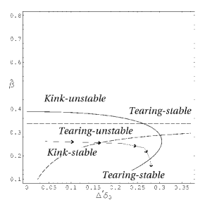
Figure 11: Boundary of marginal stability of the dissipative internal kink mode and drift-tearing mode, respectively in terms of $\hat{\beta}$ and $\delta_{0}\Delta^{\prime}$ from Eq.(99) (solid line) and from Eq. (81) (dashed lines). The parameters are the same used in Fig. 9. The kink boundary does not change significantly for $\eta_{e}<2.39.$ A schematic trajectory for the evolution of a discharge following a sawtooth crash is indicated by the line with arrows.

corresponding to windows of stability to both modes. This has a potential implication for sawtooth modelling in the spirit of Ref. (Porcelli et al., 1996), but provides more accurate stability criteria to associate with a trigger for the sawtooth crash. After such a crash, one expects a relatively rapid recovery, on the scale of the energy confinement time, of density and temperature, followed by a slower evolution of the $q$ profile on the resistive diffusion time scale. An expression for $\Delta^{\prime}$ is given by $r_{1}\Delta^{\prime}=\hat{s}_{1}^{2}/\delta\hat{W},$ where $\delta\hat{W}$ is a measure of the potential energy of the ideal internal kink mode, and $\hat{s}_{1}$ is the magnetic shear at $r_{1},$ the radial position of the $q=1$ surface. $\delta\hat{W}$ is a rather complicated function of the pressure and current profiles and, as demonstrated in Ref. (Porcelli et al., 1996), will also be a sensitive function of the pressure profile of fusion alpha particles in ITER. However, the contribution of the core plasma, as calculated in Ref. (Bussac et al., 1977) for $r_{1}/a\ll 1,$ gives

$$\delta\hat{W}\propto{\left(\frac{r_{1}}{R_{0}}\right)}^{4}\left(1-q_{0}\right)\left(\frac{13}{144}-\beta_{p}^{2}\right)$$

when $\beta_{p}$ in a measure of the poloidal $\beta$ within the $q=1$ surface. As the core plasma heats up, $\delta\hat{W}$ reduces (due to increasing $\beta_{p}$) so that, provided that $\hat{\beta}<0.4$ (see Fig. 7) there may be a period when the drift-tearing mode is unstable (a possible explanation for successor oscillations Westerhof et al. (1989) after a sawtooth crash), followed by a stable period during which the equilibrium trajectory in $(\hat{\beta},\delta_{0}\Delta^{\prime})$ (see Fig 11) passes through a region stable to both modes.

After the density and temperature profiles have recovered (we suppose this occurs before meeting the dissipative kink-instability boundary on the right of the stable region), the evolution of $\Delta^{\prime}$ will be determined by that of the $q(r)$ profile, with dependence on both $s_{1}$ (increasing $\Delta^{\prime}$) and $r_{1}$ (decreasing $\Delta^{\prime};$ however, experimental evidence suggests that the variation of $r_{1}$ during a sawtooth ramp is weak). Since $\delta_{0}\propto r_{1}/\hat{s}_{1},$ the parameter $\delta_{0}\Delta^{\prime}$ may remain fairly constant during this phase if $r_{1}$ grows only slowly relatively to $\hat{s}_{1}(t)$. However $\hat{\beta}\propto\hat{s}_{1}^{-2}$ should decrease and the equilibrium trajectory could exit the stable region in $(\hat{\beta},\delta_{0}\Delta^{\prime})$ by crossing the dissipative kink boundary, as shown schematically in Fig 11. This could represent the onset of the next sawtooth collapse phase. The sawtooth trigger can thus be deduced from Eq. (96), which resembles, but is a more precise formulation of, the stability criterion invoked by the authors of Ref. (Porcelli et al., 1996) as a prescription for a sawtooth trigger.

In summary, the stability diagram in Fig. 11 suggests a picture in which, after a sawtooth crash, there is first a period during which the drift-tearing/kinetic Alfvén wave branches may be unstable, giving rise to postcursor or successor oscillations, then a phase in which these modes are stabilised and the dissipative internal kink is not yet unstable, until finally the threshold for the latter mode is reached and a sawtooth crash ensues: a repetition of this whole cycle then begins.

The discussion above is, of course, extremely qualitative. A more meaningful technique would be to use a transport code to evolve the density, the temperature, the alpha particle population if appropriate, and the $q$ profile during a sawtooth period and follow the resulting discharge trajectory relative to the stability boundaries in Fig. 11. Here we content ourselves with simulating the evolution of the $q$ profile following a sawtooth crash, using this to calculate the evolution of $\hat{\beta}(t).$ The simulations utilise neoclassical resistivity, corrected for finite $\nu_{*e},$ the banana regime collisionality parameter, since this becomes important close to the magnetic axis (Park and Monticello, 1990). In the case of JET, $\nu_{*e}=5\times 10^{-3},$ while for ITER, $\nu_{*e}=5\times 10^{-4}.$ As an example we assume the post-crash $q$ profile is given by the Kadomtsev full reconnection model (Kadomtsev, 1976) - other models could well have been invoked, such as a partial reconnection model (Porcelli et al., 1996). We study a typical JET and ITER base-line H-mode scenario. The resulting prediction for the sawtooth periods, identified as the times that the instability boundary in Fig. 11 are reached as a result of the drop in $\hat{\beta}(t),$ are quite plausible for both JET and ITER simulations: $2$ sec for JET, and $200$ sec for ITER.

IX Discussion and Conclusions

The stability theory of the semi-collisional drift-tearing and internal kink modes, the subject of this paper, is characterised by the two key parameters, $\hat{\beta}$ and $\delta_{0}/\rho_{i}$, the latter being related to the collisionality parameter, $C$: $\delta_{0}/\rho_{i}\sim C^{1/2}$ . Semi-collisional effects are strong when $\hat{\beta}\sim\mathcal{O}(1)$ and large ion orbit effects are relevant when $\delta_{0}/\rho_{i}\ll 1$. Large, hot tokamaks such as JET and ITER operate in regimes where these conditions are satisfied. We have derived a unified theory for the stability of the modes at low $\hat{\beta}=\beta_{e}(L_{s}^{2}/L_{n}^{2})/2$ and for ion Larmor orbits much larger than the semi-collisional layer width, i.e. $\rho_{i}/\delta_{0}\gg 1$, also extending the earlier work (Pegoraro et al., 1989) on the kink mode. The effect of finite $\hat{\beta}$ on the stability of the drift-tearing and dissipative internal kink modes has then been elucidated and forms the basis for a sawtooth model.

The non-local aspects resulting from the ion orbits are accommodated by working in Fourier transform space, where the problem reduces to solving a fourth order ordinary differential equation. The problem is further simplified by exploiting the two disparate scales, $\rho_{i}$ and $\delta_{0}$, solving separately in the ‘ion region’ where the dissipative electron effects can be ignored and the ‘electron region’ where the ions can be regarded as un-magnetised. The ion region is then described by a second order differential equation in ‘$k$-space’, with the ideal MHD solution involving $\Delta^{\prime}$ providing a boundary condition at low $k$. The high-$k$ power solutions are then asymptotically matched to the similar ones emanating from the electron region solution. However, the electron region is described by a fourth order differential equation in $k$-space and it is easier to solve this by first transforming back to $x$-space, where it becomes second order, and then calculating the Fourier transform of the small $x$ asymptotic form of its solution for matching to the ion region.

The outcome at low $\hat{\beta}$ is a unified dispersion relation that encompasses the drift-tearing mode and internal kink mode. The nature of the resulting modes can be usefully parameterised in terms of $\Delta^{\prime}\rho_{i}\hat{\beta}$. At low values one finds the drift-tearing mode with frequency $\hat{\omega}\approx 1+c\eta_{e},$ where $c$ varies weakly with $\eta_{e}$ (i.e. $c$ increases from $0.7$ to $0.84$ as $\eta_{e}$ increases from small to large values), has a growth rate $\hat{\gamma}\sim(\delta_{0}/\rho_{i})(\Delta^{\prime}-\Delta_{crit}^{\prime})$ if $\Delta^{\prime}>\Delta_{crit}^{\prime}\sim\rho_{i}^{-1}\hat{\beta}\eta_{e}^{2}(\ln(\rho_{i}/\delta_{0})+c^{\prime}\eta_{e}^{1/2}),$ similar to the stabilisation by large ion orbits shown in Ref. (Cowley et al., 1986); the term proportional to the constant $c^{\prime}$ resembles that obtained for the cold ion model of Ref. (Drake et al., 1983) [see Eq. (42) for a precise description]. As $\Delta^{\prime}\rho_{i}\hat{\beta}$ increases the drift-tearing mode is affected by a kinetic Alfvén wave (KAW) propagating in the electron direction. Indeed for $\Delta^{\prime}\rho_{i}\hat{\beta}\sim\mathcal{O}(1)$ these couple strongly and there is a cross-over with an exchange of stability character: the mode identified by $\hat{\omega}\approx 1+c\eta_{e}$ becomes stable, whereas it is the KAW that becomes unstable (see Fig. 1). Near the cross-over point the growth rate is enhanced: $\hat{\gamma}\sim(\delta_{0}/\rho_{i})^{1/2}$; however, as $\Delta^{\prime}\rho_{i}\hat{\beta}$ increases further, the growth rate diminishes as $\hat{\gamma}\sim(\delta_{0}/\rho_{i})(\Delta^{\prime}\rho_{i}\hat{\beta}^{3})^{-1}$; and $\hat{\omega}\rightarrow 1$. Indeed, according to Eq. (48), when $\Delta^{\prime}$ exceeds a critical value, $\Delta_{crit}^{\prime}\sim\delta_{0}^{-1}\eta_{e}/\hat{\beta}$, it becomes stable. Stability is also ensured if $\eta_{e}>9.4$.

We have also separately examined the stability of the $\hat{\omega}\approx 1$ mode in the limit $\hat{\beta}\gg 1$ and, somewhat surprisingly, find results closely resembling those obtained in Ref. (Drake et al., 1983) for the cold ion limit: the mode is completely stabilised for all $\Delta^{\prime}$ due to shielding of the electron reconnecting layer as a result of the presence of radial gradients in the electron temperature. To elucidate the transition between instability at low $\hat{\beta}$ and stability at high $\hat{\beta}$, we have developed a treatment for finite $\hat{\beta}$, but one which is only strictly valid for a specific, though reasonable, value of $\eta_{e}$ ($\eta_{e}=2.5$). This demonstrates the onset of stabilisation due to plasma gradients when $\eta_{e}\hat{\beta}=0.85$. Below this critical value, $\hat{\beta}_{c},$ the critical $\Delta^{\prime}$ for stability is found to increase as $\hat{\beta}$ increases, as shown in Eq.(87), which is consistent with Eq.(49). A similar analytic calculation is also possible for the much larger value $\eta_{e}=9.4,$ but in this case no unstable mode is found, irrespective of the value of $\hat{\beta}.$ This is consistent with the threshold $\eta_{e}=9.4$ predicted by low $\hat{\beta}$ theory. These stability results are summarised in Fig. 7.

When the ideal internal kink mode stability parameter $\lambda_{H}=-\pi/\Delta^{\prime}r_{s}>0$, our low $\hat{\beta}$ theory recovers results of Ref. (Pegoraro et al., 1989) for the effect of the large ion orbits on the ideal internal kink mode, although the role of the small electron dissipation is somewhat different due to the improved electron model used here, which allows electron temperature perturbations and hence involves the electron temperature gradient parameter, $\eta_{e}$. When $\lambda_{H}=0$, the dissipative internal kink mode, which is related to the solution of our unified dispersion relation and whose stability depends entirely on the electron effects, remains unstable. However, we find that this mode becomes stable at a critical value of $\Delta^{\prime}$, namely $\Delta^{\prime}r_{s}\equiv-\pi/\lambda_{H}=\delta_{0}^{-1}\hat{\beta}/\ln[(\rho_{i}\hat{\beta^{2}})/\delta_{0}]$. Furthermore, if $\eta_{e}>2.38$ the mode is stable for all $\Delta^{\prime}.$

Finally we have exploited the low frequency of the dissipative internal kink mode to develop an analytic dispersion relation, valid for finite $\hat{\beta},$ to examine the effect of $\hat{\beta}$ on its stability. An analytic expression (101) for the marginally stable value can still be obtained. Although at first the critical value of $-\lambda_{H}$ reduces as $\hat{\beta}$ is increased, this trend eventually reverses and indeed all values of $-\lambda_{H}$ are unstable when $\hat{\beta}>7/18$. Figure 9 summarises these results.

The combined stability diagram for the drift-tearing mode and the dissipative internal kink mode shown in Fig. 11 provides a basis for sawtooth modelling as described in Section VIII. In the aftermath of a sawtooth crash one envisages a rapid recovery of density and temperature profiles, followed by a slower evolution of the $q$ profile. Essentially this leads to a decrease in the $\hat{\beta}$ parameter until the instability boundary for the dissipative internal kink is encountered, triggering a further crash. This could be modelled more completely with transport codes in the spirit of Ref. (Porcelli et al., 1996), but using the more precise stability criteria given in the present theory. A simulation of the time evolution of the magnetic shear using neoclassical resistivity and following its consequences for the trajectory of $\hat{\beta}(t)$ in the stability diagram, leads to plausible sawtooth periods for JET and ITER.

At this point it is helpful to highlight our key results, expressing them in terms of the parameters $\hat{\beta}$ and $\delta_{0}/\rho_{i}\propto\tau^{1/2}C^{1/2}$; the $\mathcal{O}(1)$ coefficients $c_{1}-c_{4}$ below are functions of the other parameters, $\eta_{e},$ $\eta_{i}$, and $\tau$, although we take $\tau=1$ in the evaluation of critical values of $\eta_{e}$ and $\hat{\beta}$ (more detailed descriptions of these appear in the referenced equations):

• At low $\hat{\beta}$ the drift-tearing mode with $\hat{\omega}\approx 1+0.8\eta_{e}$ is unstable for $\rho_{i}\Delta^{\prime}>c_{1}\hat{\beta}\eta_{e}^{2}\ln(\rho_{i}/\delta_{0})$ due to finite ion orbit effects [see Eq. (42)].

• At $\Delta^{\prime}\rho_{i}\hat{\beta}\sim\mathcal{O}(1)$ this mode interacts with the KAW and for larger values of this parameter it is the KAW with $\hat{\omega}\approx 1$ that is unstable, until it is stabilised when $\Delta^{\prime}>c_{2}\hat{\beta}/\delta_{0}$ [see Eq. (49)]; it is also stable for all $\Delta^{\prime}$ if $\eta_{e}>9.4.$

• For high $\hat{\beta}$ there is stability of the tearing mode for all $\Delta^{\prime}$, the transition occurring when $\hat{\beta}=c_{3}/\eta_{e}$ [see Eq. (86)]; the critical $\Delta^{\prime}$ in Eq. (49) also increases as $\hat{\beta}$ approaches this transition value, as shown in Eq. (88).

• The stability regimes of the drift-tearing and kinetic Alfvén waves in terms of $\hat{\beta}$ and $\Delta^{\prime}\rho_{i}$ are summarised in Fig. 7.

• At low $\hat{\beta}$ the dissipative internal kink mode is only unstable for $\Delta^{\prime}\rho_{i}\equiv-\pi\rho_{i}/(r_{s}\lambda_{H})>c_{4}\hat{\beta}/[\delta_{0}/\rho_{i}\ln(\hat{\beta}^{2}\rho_{i}/\delta_{0})]$ [see Eq. (96)]; it is also stable for all $\Delta^{\prime}$ if $\eta_{e}>2.4.$

• At higher $\hat{\beta}>7/18$, according to Eq. (101) there is instability for all $-\lambda_{H}$.

• Figures 9 and 10 provide stability diagrams for the drift-tearing/KAW and dissipative internal kink modes in the space of $\Delta^{\prime}$(or $-\lambda_{H}$) and $\hat{\beta}$ for higher values of $\Delta^{\prime}\rho_{i}.$

• Figure 11 suggests a resulting scenario for the onset of a sawtooth crash .

Our calculation is limited to cylindrical geometry – strictly to a sheared slab since we neglect effects of cylindrical curvature. In toroidal geometry one must take account of magnetic drifts. In the limit that the ion banana width, $w_{ban},$ is small compared to $\delta_{0},$ one can derive similar equations to those of Ref. (Drake et al., 1983), but encompassing neoclassical transport effects (Fitzpatrick, 1989, 1990). While we may neglect most of these for small values of the magnetic shear and the fraction of trapped particles, an important consequence arises from the ion neoclassical polarisation drift which reduces the parameter $C$ by a factor $B_{p}^{2}/B_{T}^{2}\ll 1,$ where $B_{p}$ and $B_{T}$ are the poloidal and toroidal magnetic fields. In the opposite limit $w_{ban}\gg\delta_{0}$ one would need to include the complete drift orbits; this calculation would be extremely complicated but can be expected to be qualitatively similar to the large ion Larmor orbit case with the substitution $\rho_{i}\rightarrow w_{ban}$. The fact that the effective value of $C$ is greatly reduced in the torus significantly extends the experimental validity of our large orbit theory.

Appendix A Internal Kink Mode

To address the case of finite $\hat{\beta}$ for the dissipative internal kink mode, we can consider the limit $|\hat{\omega}|\ll 1$, unlike the situation with the $m>1$ tearing mode which has $\omega\sim\omega_{*e}$. In the electron layer, region $2$, Eq. (15) then becomes

$$\frac{d^{2}A}{ds^{2}}=\hat{\omega}\hat{\beta}\sigma(s)A$$ (111)

where

$$\sigma(s)=\frac{1+1.71\eta_{e}+d_{1}s^{2}}{1+[d_{0}-(1+1.71\eta_{e})]s^{2}+(1+\tau)\hat{\omega}s^{4}}.$$ (112)

In the region $s\sim 1$ we can ignore the last term in the denominator and solve Eq. (111) as an expansion in $\hat{\omega},$ retaining it only for large $s\sim|\hat{\omega}|^{-1/2}$ , when it competes with the term proportional to $s^{2}$. Thus, setting $A=A_{0}$ in lowest order we find the solution even at $s=$0 to be:

$$A=A_{0}\left[1+\hat{\beta}\hat{\omega}\int_{0}^{s}ds^{\prime}(s-s^{\prime})\sigma(s^{\prime})\right].$$ (113)

At large $s$ we find

$$A\sim A_{0}\left[1+\frac{\pi}{2}\sqrt{d}\left(\frac{a}{d}-\frac{d_{1}}{d^{2}}\right)\hat{\beta}\hat{\omega}s\right]\,\,\,\mbox{for}\,\,\,s\rightarrow\infty,$$ (114)

with $a=1+1.71\eta_{e},$ $d=d_{0}-a.$ In the region $s\sim|\hat{\omega}|^{1/2},$ Eq. (111) takes the form

$$\frac{d^{2}A}{dy^{2}}=\frac{\hat{\beta}}{1+\tau}\frac{A}{1+y^{2}},$$ (115)

where $y^{2}=d^{-1}d_{1}(1+\tau)\hat{\omega}s^{2},$ with solution

$$A=b_{1}\,{}_{2}F_{1}\left(-\frac{1}{4}-\frac{\mu_{1}}{2},-\frac{1}{4}+\frac{\mu_{1}}{2};\frac{1}{2};-y^{2}\right)+b_{2}\,{}_{2}F_{1}\left(\frac{1}{4}-\frac{\mu_{1}}{2},\frac{1}{4}+\frac{\mu_{1}}{2};\frac{3}{2};-y^{2}\right),$$ (116)

where $\,{}_{2}F_{1}$ is the hypergeometric function (Abramowitz and Stegun, 1972a) and $\mu_{1}=\sqrt{1/4+\hat{\beta}/(1+\tau)}.$ Matching to solution (114) at small $y$ we have

$$\frac{b_{2}}{b_{1}}=\frac{\pi}{2}\hat{\beta}\left(a-\frac{d_{1}}{d}\right)\sqrt{\frac{\hat{\omega}}{d_{1}(1+\tau)}}.$$ (117)

To match to the ion region $1,$ we need the large $y$ limit of solution (116)

$$\begin{split}&A\sim y^{1/2+\mu_{1}}\left[1+\frac{b_{2}}{2b_{1}}\frac{\Gamma\left(\frac{3}{4}+\frac{\mu_{1}}{2}\right)}{\Gamma\left(\frac{5}{4}+\frac{\mu_{1}}{2}\right)}\frac{\Gamma\left(-\frac{1}{4}+\frac{\mu_{1}}{2}\right)}{\Gamma\left(\frac{1}{4}+\frac{\mu_{1}}{2}\right)}\right]\\ &+y^{1/2-\mu_{1}}\frac{\Gamma(-\mu_{1})}{\Gamma(\mu_{1})}\frac{\Gamma\left(\frac{3}{4}+\frac{\mu_{1}}{2}\right)}{\Gamma\left(\frac{3}{4}-\frac{\mu_{1}}{2}\right)}\frac{\Gamma\left(-\frac{1}{4}+\frac{\mu_{1}}{2}\right)}{\Gamma\left(-\frac{1}{4}-\frac{\mu_{1}}{2}\right)}\left[1+\frac{b_{2}}{2b_{1}}\frac{\Gamma\left(\frac{3}{4}-\frac{\mu_{1}}{2}\right)}{\Gamma\left(\frac{1}{4}-\frac{\mu_{1}}{2}\right)}\frac{\Gamma\left(-\frac{1}{4}-\frac{\mu_{1}}{2}\right)}{\Gamma\left(\frac{5}{4}-\frac{\mu_{1}}{2}\right)}\right].\end{split}$$ (118)

Since in the ion region we solve for the Fourier transformed current $\hat{J}(k),$ the form of $J(s)$ in the electron region can be obtained using Ampére’s law. Thus, we obtain

$$\frac{b_{-}}{b_{+}}=\left[\frac{d}{d_{1}(1+\tau)\hat{\omega}}\right]^{\mu_{1}}\frac{1/2+\mu_{1}}{1/2-\mu_{1}}\frac{\Gamma(-\mu_{1})}{\Gamma(\mu_{1})}\frac{\Gamma^{2}\left(\frac{3}{4}+\frac{\mu_{1}}{2}\right)}{\Gamma^{2}\left(\frac{3}{4}-\frac{\mu_{1}}{2}\right)}\frac{\Xi+\tan\left[\frac{\pi}{2}\left(\frac{1}{2}-\mu_{1}\right)\right]}{\Xi+\tan\left[\frac{\pi}{2}\left(\frac{1}{2}+\mu_{1}\right)\right]},$$ (119)

where

$$\Xi=\frac{1}{\pi(a-d_{1}/d)}\sqrt{\frac{d_{1}}{(1+\tau)\hat{\omega}}}\frac{\Gamma\left(\frac{1}{4}-\frac{\mu_{1}}{2}\right)}{\Gamma\left(\frac{3}{4}-\frac{\mu_{1}}{2}\right)}\frac{\Gamma\left(\frac{1}{4}+\frac{\mu_{1}}{2}\right)}{\Gamma\left(\frac{3}{4}+\frac{\mu_{1}}{2}\right)}.$$ (120)

Noting that $|\Xi|\sim|\hat{\omega}|^{-1/2}\gg 1$ when $|\hat{\omega}|\ll 1,$ in Eq. (119), we find that the low $\hat{\beta}$ limit of (119) coincides with the low $\hat{\beta}$ calculation (LABEL:eq:elsollow) at low $\hat{\omega}.$

Equation (119), after using Eq. (20), must be matched to $\hat{a}_{-}/\hat{a}_{+}$ as derived from the region $1$ solution. An analytic expression for this ratio can be obtained by iterating the solution in $|\hat{\omega}|^{2}\hat{\beta}\ll 1,$ in a similar manner to our low $\hat{\beta}$ treatment of the drift-tearing mode. Thus, in place of Eq. (8) we have

$$\frac{d}{dk}\left[\frac{G_{0}(k)}{F_{0}(k)}\frac{d\hat{J}}{dk}\right]=\hat{\omega}\hat{\beta}\frac{\hat{J}}{k^{2}},$$ (121)

where

$$G_{0}(k)=-(1-\hat{\omega}^{-1})+F_{0}(k),$$ (122)

$$F_{0}(k)=\hat{\omega}^{-1}\left\{\Gamma_{0}(k^{2}/2)-1-\eta_{i}k^{2}/2\left[\Gamma_{0}(k^{2}/2)-\Gamma_{1}(k^{2}/2)\right]\right\}$$ (123)

where we retain the $\mathcal{O}(\hat{\omega})$ correction in $G_{0}$ for large $k,$ since in this limit $F_{0}\sim k^{-1}.$ Solution (22) is then modified to give

$$\begin{split}&\hat{J}(k)=\exp\left[-\hat{\omega}\hat{\beta}\int_{0}^{k}\frac{du}{u}\frac{F_{0}(u)}{G_{0}(u)}\right]+\hat{\omega}\hat{\beta}\frac{\lambda_{H}}{\rho_{i}}\int_{0}^{k}du\frac{F_{0}(u)}{G_{0}(u)}\\ &-\left(\hat{\omega}\hat{\beta}\right)^{2}\int_{0}^{k}du\frac{F_{0}(u)}{G_{0}(u)}\int_{0}^{u}dv\frac{F_{0}(v)}{v^{2}G_{0}(v)},\end{split}$$ (124)

where we have expressed $\Delta^{\prime}$ in terms of $\lambda_{H}.$ To match solution (124) to that in region $2,$ we must first consider an intermediate large $k$ range where the approximations (122)-(123) fail: $k\sim|\hat{\omega}|^{-1}\gg 1.$ In this region

$$\frac{G_{0}}{F_{0}}=-\hat{\omega}(1+\tau)+\frac{1}{\sqrt{\pi}}\left(1-\frac{\eta_{i}}{2}\right)\frac{1}{k},$$ (125)

so that Eq. (121) can be written as

$$u(1-u)\frac{d^{2}\hat{J}}{du^{2}}-\frac{d\hat{J}}{du}+\frac{\hat{\beta}}{1+\tau}\hat{J}=0$$ (126)

where $u=\sqrt{\pi}\hat{\omega}(1+\tau)(1-\eta_{i}/2)^{-1}k,$ with solution

$$\hat{J}(k)=a_{1}\,{}_{2}F_{1}\left(-\frac{1}{2}-\mu_{1},-\frac{1}{2}+\mu_{1};1;1-u\right)+a_{2}u^{2}\,_{2}F_{1}\left(\frac{3}{2}-\mu_{1},\frac{3}{2}+\mu_{1};3;u\right).$$ (127)

[Note, the second solution is a special case, see p. 75, Eq. (7) of Ref.(Erdélyi et al., 1953)]. For $|\hat{\omega}k|\ll 1,$ i.e. $u\ll 1,$ solution (127) takes the form

$$\begin{split}\hat{J}(k)&\sim a_{1}\left\{\frac{1-(1/4-\mu^{2})u}{\Gamma\left(\frac{3}{2}+\mu_{1}\right)\Gamma\left(\frac{3}{2}-\mu_{1}\right)}+\frac{u^{2}(k_{0}-\ln u)}{2\Gamma\left(-\frac{1}{2}+\mu_{1}\right)\Gamma\left(-\frac{1}{2}-\mu_{1}\right)}+\ldots\right\}\\ &+a_{2}u^{2}(1+\ldots)\,\,\,\mbox{for\,\,\,}|\hat{\omega}k|\ll 1,\end{split}$$ (128)

with $k_{0}=\psi(1)+\psi(3)-\psi(3/2-\mu_{1})-\psi(3/2+\mu_{1}),$ where $\psi$ is the digamma function (Abramowitz and Stegun, 1972b). Expression (128) can be matched to the large $k$ limit of solution (124) gwhere the form (125) implies

$$\frac{F_{0}}{G_{0}}\approx\frac{\sqrt{\pi}}{1-\eta_{i}/2}k\left[1+\frac{\sqrt{\pi}\hat{\omega}(1+\tau)}{1-\eta_{i}/2}k\right],$$ (129)

so that

$$\begin{split}&\hat{J}(k)=1+\frac{\sqrt{\pi}\hat{\omega}\hat{\beta}}{1-\eta_{i}/2}k+\frac{\pi}{2}\left(\frac{\hat{\omega}k}{1-\eta_{i}/2}\right)^{2}\hat{\beta}(\hat{\beta}+1+\tau)\\ &-\frac{\pi}{2}\left(\frac{\hat{\omega}k\hat{\beta}}{1-\eta_{i}/2}\right)^{2}\left[\left(1-\frac{\eta_{i}}{2}\right)I_{2}+\ln k-\frac{1}{2}\right]-\frac{\sqrt{\pi}\hat{\omega}\hat{\beta}}{2(1-\eta_{i}/2)}\frac{\lambda_{H}}{\rho_{i}}k^{2},\end{split}$$ (130)

where

$$I_{2}=\frac{1}{\sqrt{\pi}}\int_{0}^{\infty}\frac{dk}{k^{2}}\left[\frac{F_{0}}{G_{0}}-\frac{\sqrt{\pi}}{1-\eta_{i}/2}\frac{k^{2}}{1+k}\right]$$ (131)

(in this integral we can take the $\hat{\omega}\rightarrow 0$ limit of $F$ anf $G$). The result of the matching is

$$\begin{split}&\frac{a_{2}}{a_{1}}=-\frac{\cos(\pi\mu_{1})}{2\pi}\left\{1-\frac{1}{\sqrt{\pi}}\frac{1-\eta_{i}/2}{1+\tau}\frac{\lambda_{H}}{\rho_{i}}\frac{1}{\hat{\omega}}-\hat{\beta}\frac{1-\eta_{i}/2}{1+\tau}I_{2}\right.\\ &\left.+\frac{\hat{\beta}}{1+\tau}\left[\frac{3}{2}-k_{0}+\ln\left(\frac{\sqrt{\pi}(1+\tau)}{1-\eta_{i}/2}\hat{\omega}\right)\right]\right\}.\end{split}$$ (132)

It remains to match the large $u$ limit of solution (127)

$$\begin{split}&\hat{J}(k)\sim\frac{\Gamma(2\mu_{1})e^{i\pi\mu_{1}}}{\Gamma\left(\frac{3}{2}+\mu_{1}\right)}\left(2\frac{a_{2}}{a_{1}}+ie^{i\pi\mu_{1}}\frac{\hat{\beta}}{1+\tau}\right)u^{1/2+\mu_{1}}\\ &+\frac{\Gamma(-2\mu_{1})e^{-i\pi\mu_{1}}}{\Gamma\left(\frac{3}{2}-\mu_{1}\right)}\left(2\frac{a_{2}}{a_{1}}+ie^{-i\pi\mu_{1}}\frac{\hat{\beta}}{1+\tau}\right)u^{1/2-\mu_{1}},\end{split}$$ (133)

to the region $2$ solution. Reintroducing $k$, Eq. (133) provides the ratio $\hat{a}_{2}/\hat{a}_{1}$ to be matched to $\hat{c}_{+}/\hat{c}_{-}$ as given by Eqs. (119) with the help of Eq. (20), i.e.

$$\frac{\hat{c}_{-}}{\hat{c}_{+}}=\frac{\Gamma\left(-\frac{1}{2}+\mu_{1}\right)}{\Gamma\left(-\frac{1}{2}-\mu_{1}\right)}\tan\left[\frac{\pi}{2}\left(\frac{1}{2}+\mu_{1}\right)\right]\frac{b_{+}}{b_{-}}.$$ (134)

This yields the final dispersion relation

$$\begin{split}\left[\frac{e^{-i\frac{5}{4}\pi}}{8\sqrt{\pi}\hat{\omega}}\frac{\delta_{0}}{\rho_{i}}\sqrt{\frac{d(\eta_{e})}{d_{1}}}\,\frac{1-\eta_{i}/2}{(1+\tau)^{3/2}}\right]^{2\mu_{1}}\times\frac{\Xi(\hat{\omega})+\tan\left[\frac{\pi}{2}\left(\frac{1}{2}-\mu_{1}\right)\right]}{\Xi(\hat{\omega})+\tan\left[\frac{\pi}{2}\left(\frac{1}{2}+\mu_{1}\right)\right]}=&\\ \frac{1/2-\mu_{1}}{1/2+\mu_{1}}\frac{\Gamma^{2}(\mu_{1})}{\Gamma^{2}(-\mu_{1})}\frac{\Sigma(\hat{\omega})+i\frac{\hat{\beta}}{1+\tau}e^{i\pi\mu_{1}}}{\Sigma(\hat{\omega})+i\frac{\hat{\beta}}{1+\tau}e^{-i\pi\mu_{1}}},&\end{split}$$ (135)

where $\Sigma(\hat{\omega})=2a_{2}/a_{1}.$ We note that we can simplify Eq. (135) since $|\Xi(\hat{\omega})|\propto\left|\hat{\omega}\right|^{-1/2}\gg 1,$ as given by Eq. (120),

$$\left[\frac{e^{-i\frac{5}{4}\pi}}{8\sqrt{\pi}\hat{\omega}}\frac{\delta_{0}}{\rho_{i}}\sqrt{\frac{d(\eta_{e})}{d_{1}}}\,\frac{1-\eta_{i}/2}{(1+\tau)^{3/2}}\right]^{2\mu_{1}}=\frac{1/2-\mu_{1}}{1/2+\mu_{1}}\frac{\Gamma^{2}(\mu_{1})}{\Gamma^{2}(-\mu_{1})}\frac{\Sigma(\hat{\omega})+i\frac{\hat{\beta}}{1+\tau}e^{i\pi\mu_{1}}}{\Sigma(\hat{\omega})+i\frac{\hat{\beta}}{1+\tau}e^{-i\pi\mu_{1}}}.$$ (136)

Equation (136) provides a finite $\hat{\beta}$ dispersion relation for the dissipative internal kink mode, where we recall $\delta_{0}/\rho_{i}\ll 1$ and $\mu_{1}$ is independent of $\hat{\omega}.$

References

- Furth et al. (1963) H. P. Furth, J. Killeen, and M. N. Rosenbluth, Phys. Fluids 6, 1169 (1963).
- Hastie (1998) R. J. Hastie, Astrophys. Space Sci. 256, 177 (1998).
- Coppi et al. (1976) B. Coppi, R. M. O. Galvao, R. Pellat, M. N. Rosenbluth, and P. H. Rutherford, Fiz. Plazmy 6, 691 (1976), Sov. J. Plasma Phys. Vol. 11 p. 226 (1975).
- Migliuolo et al. (1991) S. Migliuolo, F. Pegoraro, and F. Porcelli, Phys. Fluids B 3, 1338 (1991).
- Porcelli et al. (1996) F. Porcelli, D. Boucher, and M. N. Rosenbluth, Plasma Phys. and Control. Fusion 38, 2163 (1996).
- Pegoraro and Schep (1986) F. Pegoraro and T. J. Schep, Plasma Phys. and Control. Fusion 28, 647 (1986).
- Pegoraro et al. (1989) F. Pegoraro, F. Porcelli, and T. J. Schep, Phys. Fluids B 1, 364 (1989).
- Jardin et al. (1993) S. Jardin, M. Bell, and N. Pomphrey, Nucl. Fusion 33, 371 (1993).
- Cole and Fitzpatrick (2006) A. Cole and R. Fitzpatrick, Phys. Plasmas 13, 032503 (2006).
- Cole et al. (2007) A. J. Cole, C. C. Hegna, and J. D. Callen, Phys. Rev. Lett. 99, 065001 (2007).
- Evans et al. (2004) T. E. Evans, R. A. Moyer, P. R. Thomas, J. G. Watkins, T. H. Osborne, J. A. Boedo, E. J. Doyle, M. E. Fenstermacher, K. H. Finken, R. J. Groebner, et al., Phys. Rev. Lett. 92, 235003 (2004).
- Glasser et al. (1975) A. H. Glasser, J. M. Greene, and J. L. Johnson, Phys. Fluids 18, 875 (1975).
- Bussac et al. (1977) M. N. Bussac et al., Plasma Physics and Control. Nucl. Fusion Research 1, 269 (1977), proc. IAEA Int. Conf. Berchtesgaden, 1976.
- Rutherford and Furth (1971) P. H. Rutherford and H. P. Furth, Princeton Plasma Physics Laboratory Report MATT-872 (1971).
- Drake and Lee (1977) J. F. Drake and Y. C. Lee, Phys. Fluids 20, 1341 (1977).
- Chang et al. (1981) C. S. Chang, R. R. Dominguez, and R. D. Hazeltine, Phys. Fluids 24, 1655 (1981).
- Coppi et al. (1979) B. Coppi, J. W. Mark, L. Sugiyama, and G. Bertin, Ann. Phys. 119, 370 (1979).
- Drake et al. (1983) J. F. Drake, J. T. M. Antonsen, A. B. Hassam, and N. T. Gladd, Phys. Fluids 26, 2509 (1983).
- Grasso et al. (2001) D. Grasso, M. Ottaviani, F. Porcelli, Phys. Plasmas 8, 4306 (2001).
- Fitz (2010) R. Fitzpatrick, Phys. Plasmas 17, 042101 (2010).
- Grasso et al. (2002) D. Grasso, M. Ottaviani, F. Porcelli, Nucl. Fusion 42, 1067 (2002).
- Bussac et al. (2002) M.N. Bussac, R. Pellat, J.L. Soule, Phys. Rev. Lett. 40, 1500 (1978).
- Nishmura et al. (2007) S. Nishimura, M. Yagi, S. Itoh, M. Azumi, K. Itoh, J. Phys. Soc. Jap. 10, 0645011 (2007).
- Hahm and Chen (1986) T. S. Hahm and L. Chen, Phys. Fluids 29, 1891 (1986).
- Yu et al. (2002) Q. Yu, S. Gunter, B.D. Scott, Phys. Plasmas 10, 797 (2002).
- Antonsen and Coppi (1981) T. M. Antonsen and B. Coppi, Phys. Lett. A 81, 335 (1981).
- Hahm and Chen (1985) T. S. Hahm and L. Chen, Phys. Fluids 28, 3061 (1985).
- Hahm (1984) T. S. Hahm, PhD Thesis, Princeton University (1984).
- Cowley et al. (1986) S. C. Cowley, R. M. Kulsrud, and T. S. Hahm, Phys. Fluids 29, 3230 (1986).
- Pegoraro and Schep (1981) F. Pegoraro and T. J. Schep, Phys. Fluids 24, 478 (1981).
- Ara et al. (1978) G. Ara, B. Basu, B. Coppi, G. Laval, M. N. Rosenbluth, and B. V. Wadell, Ann. Phys. 112, 443 (1978).
- Abramowitz and Stegun (1972a) M. Abramowitz and I. A. Stegun, Handbook of Mathematical Functions, Chapter 15 (National Bureau of Standards Applied Mathematics, 1972a).
- Abramowitz and Stegun (1972b) M. Abramowitz and I. A. Stegun, Handbook of Mathematical Functions, Chapter 6 (National Bureau of Standards Applied Mathematics, 1972b).
- Abramowitz and Stegun (1972c) M. Abramowitz and I. A. Stegun, Handbook of Mathematical Functions, Chapter 10 (National Bureau of Standards Applied Mathematics, 1972c). quista
- Westerhof et al. (1989) E. Westerhof and P. Smeulders, Nucl. Fusion 29, 1056 (1989).
- Park and Monticello (1990) W. Park and D. Monticello, Nucl. Fusion 30, 2413 (1990).
- Kadomtsev (1976) B. B. Kadomtsev, Sov. Phys. JETP 1, 389 (1976).
- Fitzpatrick (1989) R. Fitzpatrick, Phys. Fluids B 1, 2381 (1989).
- Fitzpatrick (1990) R. Fitzpatrick, Phys. Fluids B 2, 2636 (1990).
- Erdélyi et al. (1953) A. Erdélyi, W. Magnus, F. Oberhettinger, and F. G. Tricomi, Higher Trascendental Functions, vol. 1 (McGraw-Hill Book Company, Inc, New York, 1953).