Levy process simulation by stochastic step functions

Abstract

We study a Monte Carlo algorithm for simulation of probability distributions based on stochastic step functions, and compare to the traditional Metropolis/Hastings method. Unlike the latter, the step function algorithm can produce an uncorrelated Markov chain. We apply this method to the simulation of Levy processes, for which simulation of uncorrelated jumps are essential.

We perform numerical tests consisting of simulation from probability distributions, as well as simulation of Levy process paths. The Levy processes include a jump-diffusion with a Gaussian Levy measure, as well as jump-diffusion approximations of the infinite activity NIG and CGMY processes.

To increase efficiency of the step function method, and to decrease correlations in the Metropolis/Hastings method, we introduce adaptive hybrid algorithms which employ uncorrelated draws from an adaptive discrete distribution defined on a space of subdivisions of the Levy measure space.

The nonzero correlations in Metropolis/Hastings simulations result in heavy tails for the Levy process distribution at any fixed time. This problem is eliminated in the step function approach. In each case of the Gaussian, NIG and CGMY processes, we compare the distribution at $t=1$ with exact results and note the superiority of the step function approach.

Keywords: Levy process, Markov chains, Monte Carlo methods, Simulation of Probability Distributions

MSC2010: 60G51, 65C05, 60G17, 62M10, 60J22, 60J75

1 Introduction

Levy processes are a type of stochastic process whose paths can behave erratically like a Brownian motion, as well as include discontinuities, i.e. jumps. Many observed phenomena in nature and human society display continuous erratic motion similar to Brownian motion, while also having random jumps at random times, and can therefore be modelled using Levy processes. Areas of application include e.g. microscopic physics, chemistry, biology and financial markets. Therefore the study of computer simulation methods for Levy processes is an important subject.

In our case, will will employ a jump-diffusion approximation when we apply our method to infinite activity Levy processes. Jump-diffusion processes can be considered as a sum of three independent component processes. A deterministic drift, a Brownian motion, and lastly a finite activity jump process. The jump process is completely described by a Levy measure $\nu$ on $\mathbb{R}$. The average jump rate, or intensity, is given by the total weight $\lambda:=\nu(\mathbb{R})$, and the distribution of jump values follows the Levy probability measure $\nu_{1}:=\nu/\lambda$.

By definition, the Brownian motion has independent increments, and this is also the case for subsequent jumps in the jump process. In computer simulations, violation of these properties will give incorrect results. Simulation of the Brownian motion is easy, since well known algorithms exist for producing uncorrelated draws from a normal distribution, using a good pseudo-random number generator (PRNG).

On the other hand, the simulation of the jump process requires more care. In principle we can obtain uncorrelated draws from $\nu_{1}$ by inverting its cumulative distribution function. However, this might not be feasible to do for a given $\nu_{1}$. In this case, the Metropolis/Hastings (MH) algorithm might come to the rescue. It can easily produce a Markov chain with values distributed according to $\nu_{1}$. However, subsequent values will be correlated, as described below.

In this paper we propose an algorithm to produce uncorrelated jumps along each path, without generating such a multitude of Markov chains. This method is based on stochastic step functions (SF), which will be defined below. As opposed to MH, it is not an accept/reject algorithm. Therefore it is able to generate an uncorrelated chain of values distributed according to any given probability measure. We will test this algorithm in jump-diffusion computer simulations and compare with MH. We apply the simulation techniques to a Gaussian process, for which the exact distribution at $t=1$ is known. Convergence towards this exact result is studied.

We also consider adaptive variants of these algorithms. For these, we subdivide $\mathbb{R}$ into appropriate regions, and generate a discrete distribution that allows us to efficiently draw among these regions in an uncorrelated way. As the simulation progresses, this discrete distribution is adaptively improved. The calculation of the jump rate $\lambda$ is also adaptively improved.

As an interesting application of these simulation techniques, we also look at infinite activity pure jump processes, which are also a Levy process subclass. Here, motion occurs in the form of an infinitude of discontinuous jumps. Some of these processes can be approximated by jump-diffusion by substituting the smallest jumps for an appropriate Brownian motion [1]. The examples we focus on are the NIG and CGMY processes.

In section 2 we review the elementary facts about jump-diffusion processes. In section 3 we describe the relevant simulation methods, and discuss their pros and cons, as well as provide results from numerical experiments. In section 4 we describe our probability space subdivision method and the accompanying adaptability properties of the algorithms, and study the efficiency and correlation strengths of different algorithms by simulation from a Gaussian distribution. We then proceed in section 5 to perform simulations of jump-diffusion processes. We notice how the MH correlations adversely affect the distribution of the simulated process, and compare the SF and MH algorithms for simulation of a process with a Gaussian Levy measure. Lastly, in section 6, we review the jump-diffusion approximation of infinite activity pure jump processes, and apply our simulations techniques on the infinite activity NIG and CGMY processes, in order to compare algorithms in these interesting cases.

2 Jump-diffusion processes

First we review some elementary facts about real-valued jump-diffusion Levy processes on a time interval $[0,T]$. Such a process can be expressed as a sum of three simple components

$$L_{t}=\mu t+B_{t}+J_{t}.$$ (1)

The first part is a deterministic drift with rate $\mu$, $B_{t}$ is Brownian motion, and $J_{t}$ is a compound Poisson process. The latter describes completely the discontinuities (jumps) of the paths of $L_{t}$, by means of a Levy measure $\nu$ on $\mathbb{R}$. We will several times abuse notation by writing $\nu$ both for the Levy measure and its density. Firstly, this measure determines the jump intensity (jump rate)

$$\lambda:=\nu(\mathbb{R})<\infty,$$ (2)

of $L_{t}$. Secondly, the corresponding Levy probability measure

$$\nu_{1}:=\nu/\lambda,$$ (3)

determines the distribution of jump sizes. Note that we do not have $E[L_{t}]=\mu t$ in general, although this is satisfied in our examples.

Now, $J_{t}$ can be expressed as

$$J_{t}=\sum_{j=1}^{N_{t}}V_{j},$$ (4)

where $N_{t}$ is a Poisson process of intensity $\lambda$, and the jumps $\{V_{j}\}$ are indendent random variables distributed according to the Levy probability measure. We do not simulate the Poisson process $N_{t}$ directly. Instead, for each path we draw the total number of jumps individually from an exponential distribution with average $\lambda T$. Then we randomly distribute those jumps on $[0,T]$. We will choose $T=1$ for our simulations. The lengths of consecutive time intervals between jumps will be independent and exponentially distributed, and give the correct jump intensity. This is described in [3].

Note that for a general Levy process $\lambda$ is in general not finite, because the Levy measure might diverge too strongly towards the origin. However, the following condition always holds,

$$\int_{\mathbb{R}}\min(1,s^{2})\nu(ds)<\infty.$$ (5)

which restricts the strength on the divergence of $\nu$ at the origin.

The difficulty in simulation is to draw independent jump values from $\nu_{1}$. We will generate a Markov chain with $\nu_{1}$ as its invariant measure. However, it is essential for correct simulation that jumps along each path are uncorrelated. Note that existence of correlations between jumps in different paths will not ruin the convergence in distribution, but only slow it down.

For a Markov chain $\{X_{i}\}$, we define the sequential correlation as

$$c:=\mathrm{E}[(X_{i+1}-\bar{X})(X_{i}-\bar{X})]/\sigma^{2},$$ (6)

where $\bar{X}$ is the Markov chain average and $\sigma^{2}$ is its standard deviation,

$$\bar{X}:=E[X],\quad\sigma^{2}:=E[X^{2}-\bar{X}^{2}].$$

3 Simulation of a probability measure

To simulate the jumps, we must draw independent values from $\nu_{1}$. In cases where $\nu_{1}$ is complicated, it is common to use the Metropolis/Hastings (MH) algorithm [7, 4]. This method generates a Markov chain with $\nu_{1}$ as its invariant density. Unfortunately, the Markov chain often has large correlations between successive values. Successive values in such a chain cannot be used to represent jumps within a single jump-diffusion path.

It is possible to reduce this problem by several methods. One is to skip a number of terms in the Markov chain to reduce correlation. This results in a loss of efficiency. Another method is to generate multiple independent Markov chains. Each jump-diffusion path then uses values from different Markov chains. This will lead to a correct pathwise simulation, and therefore correct convergence in distribution. The correlations will in this case only slow down the convergence.

We will look at two methods, MH and one based on stochastic step fuctions (SF). Both rely on a transition probability distribution $\rho$ to determine upcoming values from the previous one. We say that we are dealing with a local algorithm if $\rho$ is localized around the current value. An independent algorithm results if $\rho$ is independent of the current position.

Use of an independent MH algorithm can reduce correlations dramatically if one is able to find a $\rho$ that approximates $\nu_{1}$. The downside is that efficiency will suffer if $\rho$ is not computationally simple. We will focus on generation of low correlation Markov chains in order to get by using only one chain for the Levy process jumps.

3.1 Metropolis/Hastings (MH)

The well-known MH algorithm generates a realisation $\{x_{i}\}$ of a Markov chain distributed according to $\nu_{1}$. Its most popular incarnation is local, where the transition probability density $\rho(x_{i},x_{i+1})$ involved in each transition $x_{i}\mapsto x_{i+1}$ is localized around the value $x_{i}$, and its width is adjusted to give an average acceptance rate somewhere around $1/2$. The resulting correlation between successive values can be classified into two types:

• Rejection correlation: Since both the local and independent algorithms are based on acceptance/rejectance, correlations are introduced by repeated values due to rejections. With an acceptance rate around $1/2$, repeated values will often occur.

• Transition correlation: In order for the local algorithm to be efficient, its transition probability measure $\rho(x_{i},x_{i+1})$ must in many cases be quite strongly localized; otherwise too small an acceptance rate will result. Thus the difference between subsequent variates of the Markov chain will tend to be small.

To reduce transition correlation, the width of the transition distribution can be increased. But this typically leads to a reduced acceptance ratio, which gives an increased rejection correlation, and vice versa.

As a numerical example, consider a unit variance normal distribution, simulated with a simple localized uniform transition probability measure. The correlation defined in (6) as a function of transition probability width is displayed in Figure 1. As expected, the correlation has a minimum. Towards smaller widths the transition correlation increases, and towards larger widths the rejection correlation increases. Thus there is a lower bound on the amount of correlation for this algorithm, and it seems that the local MH algorithm is therefore not suited for our purposes. We will from now on focus on the independent MH algorithm.

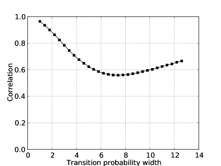
Figure 1: Correlation $c$ versus transition probability width $w$ for the local MH algorithm, in a simulation of the unit normal distribution using a uniform centered transition probability distribution. Correlation is minimal around $w\approx 7$, where $c\approx 0.55$.

3.2 Stochastic step function (SF)

Next, we propose a simulation algorithm based on stochastic step functions, that can be adjusted to completely eliminate correlations. This possibility of vanishing correlations is an attractive property that allows it to be used as a reference algorithm. It can also be adjusted to run more efficiently, with nonzero correlation.

Let us give a pathwise definition of the SF process on $[0,\infty)$ for some measure density $\nu$ on $\Omega\subset\mathbb{R}$, not necessarily normalized. Consider a sequence $\{\tau_{i}\}_{i=0}^{\infty}\subset(0,\infty)$ of resting times and corresponding jump times $\{t_{i}\}_{i=0}^{\infty}$, defined recursively by

$$t_{0}=0,\quad t_{i+1}:=t_{i}+\tau_{i}.$$

In addition, let $\{s_{i}\}_{i=0}^{\infty}\subset\Omega$ be a Markov chain with initial value $s_{0}=0$ and transition probability density $\rho(s_{i},s_{i+1})$. Assume that $\rho(s_{i},\cdot)$ is absolutely continuous with respect to the Lebesgue measure on $\mathbb{R}$, and homogeneous, i.e. it can be expressed as $\rho(s_{i+1}-s_{i})$.

From this data, we are now ready to define our stochastic step function process $X_{t}$, by defining its paths as the piecewise constant cadlag functions (right-continuous with left limits) of the form

$$X_{t}=\sum_{i=1}^{\infty}s_{i}\chi_{I_{i}}(t),\quad I_{i}:=[t_{i},t_{i+1}),$$

where $\chi_{I}$ is the indicator function for the interval $I$, and where the resting times are given by $\tau_{i}:=\nu(s_{i})$.

We see that the paths of $X_{t}$ linger for a some time at each of its attained positions, with a resting time equal to the local value of the density $\nu$. Consider the graph of such a path on $[0,T]$ for large $T$ compared to $\sup\nu$. As $T$ increases, the relative path length within a given subset $A\subset\Omega$ on the vertical axis converges towards $\nu(A)/\nu(\Omega)=:\nu_{1}(A)$. When sampling this path on a uniform time-grid, the obtained values will therefore be distributed according to the probability density $\nu_{1}$.

As in the case of local MH, we get transition probability correlations if $\rho$ is localized. In this algorithm, however, there is no accept/reject step, and therefore no rejection correlation. As an example, let us choose $\rho$ to be the uniform probability distribution on $\Omega$. As noted above, if we sample the step function path generated above on a uniform time grid, we get a chain of values distributed according to $\nu_{1}$. If we make sure that the time discretization interval size $\Delta t$ is larger than $\sup\nu$, repeated values will never occur and there are no correlations.

Note that as in MH algorithms, we do not need to know scale factor relating $\nu_{1}$ and $\nu$. If $\sup\nu$ is initially unknown, we can simply start with any estimate, and improve it adaptively as the algorithm runs.

It is easy to see that the amount of computer time spent between each discrete time value is proportional to $\sup\nu/\nu(\Omega)$ in its correlation-free mode. If this ratio is large, the algorithm will be inefficient.

One can make the time discretization finer to increase the rate of variate generation, but this introduces correlations since values for which $\nu$ is large will be repeated with complete certainty. This is similar to the Metropolis algorithm, where values of large $\nu$ are repeated (although not with complete certainty). The SF algorithm can be made less deterministic in this case by letting the resting times be random variables distributed according to an exponential distribution with mean $\nu(x)$, where $x$ is the current position.

Since we are concerned with minimizing correlations in the context of jump-diffusion simulations, we will use independent algorithms, where $\rho(x_{i},x_{i+1})$ is independent of $x_{i}$.

3.3 Simulation comparison

Let us illustrate the advantages of the local SF algorithm over local MH by considering an example with a probability distribution with several modes on a sample space $\Omega=[0,1]$. Our goal is to simulate values from a probability distribution proportional to the following unnormalized density with two strong modes,

$$\nu(x)=\left\{\begin{array}[]{ll}1&,x\in[0,0.25)\cup[0.5,0.75)\\ 0.01&,\mbox{otherwise}.\end{array}\right.$$ (7)

For both MH and SF, we used a localized uniform transition probability density $\rho$ of width $1/2$. For MH, this gave an acceptance rate of approximatively 0.55. The SF Markov chain realisation was obtained by sampling the stochastic step function using a lattice spacing slightly larger than $\sup\nu$ in order to avoid any repeating values.

The results are shown in Figure 2. One sees immediately that the MH algorithm has the potential of getting stuck inside a mode for long periods. This is caused by rejection correlation as found in accept/reject algorithms such as MH. On the other hand, the SF algorithm has no such problems since it lacks such correlations. This serves to illustrate a problem that often can occur with MH. The SF algorithm is a clear favourite in this case if mixing is important for the application of these Markov chains.

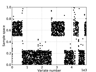
(a) Local MH

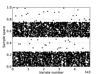
(b) Local SF

Figure 2: Markov chain realisations using local MH and local SF. The SF algorithm mixes much better than MH.

4 Probability space subdivision and adaptability

The Levy probability measure from which we will simulate in the context of jump-diffusions will often be defined on the unbounded probability space $\Omega=\mathbb{R}$. This presents no difficulty for the MH algorithm. SF algorithms on the other hand need to impose upper and lower cutoffs on $\Omega$, in order to avoid step functions that diverge towards infinity. For simplicity, we impose such cutoffs on both algorithms in our examples. Alternatively, one could perform a topology-changing coordinate transformation on $\Omega$ to obtain a compact space, however we will not do this in our examples. From now on we therefore assume $\Omega\subset\mathbb{R}$ to be a bounded interval which we choose symmetrically about the origin. We will only deal with symmetrical Levy measures in our examples.

In order to reduce correlations in the MH algorithms, and increase efficiency in the SF algorithms, we define a finite disjoint subdivision $\{U_{i}\}$ of $\Omega$, where $\cup_{i}U_{i}=\Omega$. We construct a discrete distribution $\tilde{\nu}$ on the finite set $\{U_{i}\}$. For each $U_{i}\subset\Omega$, the value $\tilde{\nu}(U_{i})$ must approximate $\nu(U_{i})$, i.e. the Levy measure weight of $U_{i}$. The simulation algorithm starts with a preliminary estimate of $\tilde{\nu}$ which is adaptively improved throughout the simulation, as explained below in the two cases of MH and SF. This is reminiscent of variance reduction schemes used in Monte Carlo integration, such as stratification and the VEGAS algorithm [5]. We now describe in more details how this is done in each case.

4.1 Adaptive Independent MH (AIMH)

As explained above, we will use an independent MH algorithm. The independent transition probability $\rho$ is defined as follows. First, use the discrete unnormalized probability measure $\tilde{\nu}$ to draw a subset $U_{i}$. Then a random position within this subdomain is proposed and the value of $\nu$ at this position is calculated. Thereafter follows the usual MH accept/reject step.

The initial draw of $U_{i}$ is done without introducing correlations, using e.g. an efficient algorithm which is independent of the normalization of $\tilde{\nu}$ [8]. The registered values of $\nu$ are accumulated, and used periodically in the simulation to improve $\tilde{\nu}$. Essentially, a separate Monte Carlo simulation is being performed within each subdomain $U_{i}$ to improve the discrete distribution $\tilde{\nu}$, while the algorithm proceedes to generate new draws from $\nu$.

Since subdomains $U$ of $\Omega$ are drawn by means of $\tilde{\nu}$ without introducing correlations, the amount of correlation generated by the algorithm as a whole is reduced. Transition correlation is completely eliminated since since the algorithm is independent. It is impossible to completely eliminate rejection correlation in an MH algorithm unless $\rho$ is identical to $\nu_{1}$. However, since $\nu$ is well approximated on each subdomain (as long as the subdivision is sufficiently fine), these will be small, and the acceptance rate will be high. As $\tilde{\nu}$ adapts, the acceptance rate rises and correlation decreases. The subdivision discretization implies a lower bound for the amount of correlation. But this is still a big improvement on a basic local MH algorithm for the cases we consider. Note that the subdivision cannot be made arbitrarily fine, since the discrete algorithm will then become inefficient.

4.2 Adaptive Independent SF (AISF)

It is possible to improve the efficiency of the SF algorithm by a similar construction, without introducing correlations. In this case, the SF algorithm proceeds as follows. First draw a subdomain $U_{i}$ using $\tilde{\nu}$. Draw a random position $x$ within this subdomain, and record the value $\nu(x)$ for later use to improve $\tilde{\nu}$. For each subset $U_{i}$ we keep an estimate of $\sup_{i}\nu$ which is updated for each sample. Each subset is also accompanied by a local time variable $t_{i}$. For each position $x$ within $U_{i}$, we increase $t_{i}$ by the resting time $\nu(x)$. We choose new positions independently within $U_{i}$ until $t_{i}$ exceeds the current estimate of $\sup_{i}\nu$.

When the above loop exists, we have determined our new position and we subtract $\sup_{i}\nu$ from $t_{i}$ in anticipation of the next time we enter $U_{i}$. In a sense we are using a different time discretization in each subset $U_{i}$ of $\Omega$.

This modified algorithm avoids spending a lot of time in areas of low probability for two reasons. First, the low probability subdomains will rarely be entered when drawing from the dicrete distribution $\tilde{\nu}$. Secondly, the amount of time necessary to exit the loop in those regions is much smaller, since the local $\sup\nu$ is small. By exploiting the subdivision of $\Omega$, and using an efficient algorithm for drawing from discrete distributions, we improve the efficiency of the SF algorithm drastically in nontrivial cases.

Both $\tilde{\nu}$ and the estimates $\sup\nu$ are adaptively improved throughout the simulation.

4.3 Simulation test

To check the rate of convergence of the differerent methods, we simulated from a Gaussian distribution with unit variance. The rate of variate generation, correlation, and the convergence towards the known exact result were analyzed.

A histogram of the simulated values is gathered, and compared with a histogram calculated from the Gaussian distribution. We define the histogram error using an $L^{\infty}$ measure, i.e. as the absolute value of the maximum deviation from the exact result. The plots show the histogram error as a function of simulation running time. The simulations were run on one core of an Intel T4400 laptop processor, but only the relative efficiencies matter here. Results are shown in Figure 3 and are discussed below.

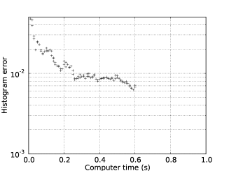
(a) Local MH

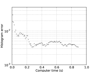
(b) AIMH

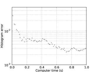
(c) Local SF

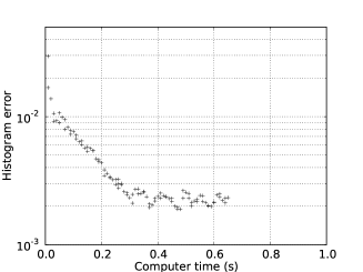
(d) AISF

Figure 3: Histogram error versus computer time, for simulation from normal distribution.

4.3.1 Local MH

Since a low correlation will be important for our later use on Levy processes, we selected the transition probability width $0.75$, giving the minimal correlation of approximatively 0.55, according to Figure 1. The variate generation rate was approximately $3.4\cdot 10^{6}/s$ in this case.

4.3.2 AIMH

As expected, as great improvement of the correlation was obtained compared to local MH. Since the algorithm is more complicated, the variate generation rate decreased to $2.3\cdot 10^{6}/s$, or roughly $60\%$ of local MH. However, the correlation was reduced to around 0.03. This dramatic decrease results in a faster histogram convergence in terms of computer time. The lower correlation nature of this algorithm will be noticeably beneficial when simulating Levy processes.

4.3.3 Local SF

We adjusted the basic SF algorithm parameters to give zero correlation, and used a uniform transition probability density on $[-5,5]$. Thus we are running it quite inefficiently as regards variate generation speed, which turned out to be around $1.4\cdot 10^{6}/s$. Despite this, the histogram converges faster than local MH, due to the lack of correlation.

4.3.4 AISF

As expected, when including the domain subdivision and adaptive algorithm, the SF algorithm efficiency increased (in fact doubled) with a variate generation rate of $3.1\cdot 10^{6}/s$. The amount of correlation here is still zero, which leads to the fastest histogram convergence. So this is a great improvement at no cost other than increased algorithm complexity. It is perfectly suited for simulating consecutive jumps in jump-diffusion process paths.

5 Jump-diffusion simulation

As previously mentioned, existence of correlations among jumps within the same jump-diffusion path is disastrous. Let us check this by using an local MH algorithm to simulate an exactly solvable stochastic process [6] and compare distributions at $t=1$. It is defined as

$$X_{t}:=\sigma W_{t}+J_{t},$$

$$J_{t}=\sum_{i=1}^{N_{t}}Y_{i},\quad Y_{i}\sim N(\mu,\delta^{2}),\quad\mu,\delta\in\mathbb{R},$$

where $N_{t}$ is a Poisson process of intensity $\lambda$. We choose $\sigma=1$, $\mu=0$, $\delta=1$, and $\lambda=10$ in order to get an appreciable number of jumps within the time domain $[0,1]$.

The exact PDF of this process for $t>0$ is [3, Eq.(4.12)]

$$p_{t}(x)=\exp(-\lambda t)\sum_{k=0}^{\infty}\frac{(\lambda t)^{k}\exp(-\frac{x^{2}}{2(t+k)})}{k!\sqrt{2\pi(t+k)}}.$$

For local MH simulations, the positive correlations between subsequent jumps leads to heavy distribution tails. Results confirming this are shown in Figure 4. The simulation of the jumps used a localized uniform transition probability of width 4, which resulted in a MH acceptance rate of around 0.56.

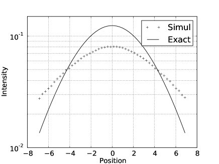
Figure 4: Local MH simulation of distribution at $t=1$ of Gaussian process, and exact result. Due to jump correlations, the simulated histogram has heavy tails.

We now turn to our serious attemps at jump-diffusion simulation. We have simulated the same process using AIMH and AISF algorithms. In this case we use the already known value of $\lambda=10$ in the simulations, so the adaptability consists solely of the calculation of the discrete subdivision distribution, and in the AISF case also of the local subdivision supremum calculations. As opposed local MH, in this case the distribution at $t=1$ approaches the exact curve, as seen in Figure 5. Note that despite our use of upper/lower cutoffs in the implementation of the discrete subdivision, the tails of the local MH simulation are still somewhat heavy.

We use the same $L^{\infty}$ measure of convergence detailed above. Convergence results are shown in Figure 6. The AISF outperforms the AIMH algorithm due to its lower correlation which leads to faster and more accurate convergence.

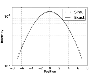
(a) AIMH

(b) AISF

Figure 5: Distributions of Gaussian process at $t=1$ for AIMH and AISF simulations. The continuous curve represents the exact result. Notice the slight heavy tails in the AIMH case, due to nonzero jump correlations.

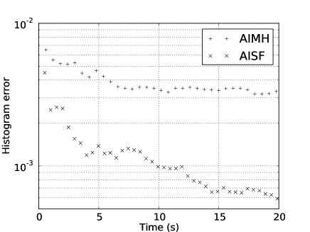
Figure 6: Error in distribution at $t=1$ for the Gaussian process, versus computer simulation time. AISF gives the fastest convergence. The AIMH heavy tails cause a lower bound on the error.

6 Application to NIG and CGMY infinite activity pure jump processes

We present two applications within the realm of infinite activity pure jump Levy processes, namely NIG and CGMY. To this end, we employ the jump difffusion approximation of these processes [1].

6.1 Jump-diffusion approximation

For an infinite activity Levy process, the intensity $\lambda$ is undefined, since its defining integral (2) diverges. However, by virtue of (5), it is possible to approximate the infinitude of small jumps by a Brownian motion process. Consider an infinite activity pure jump Levy process $L_{t}$. For $\epsilon>0$, define the following subsets of $\Omega$,

$$A^{\epsilon,-} := \{|x|<\epsilon:x\in\mathbb{R}\}$$

$$A^{\epsilon,+} := \{|x|>\epsilon:x\in\mathbb{R}\}.$$

These represent small and large jumps, respectively.

We now define the unique Levy measures $\nu^{\epsilon,-}$ and $\nu^{\epsilon,+}$ on these subdomains as follows. For any $\nu$-measurable $U\subset\mathbb{R}-\{0\}$, define

$$\nu^{\epsilon,-}(U) := \nu(U\cap A^{\epsilon,-})$$

$$\nu^{\epsilon,+}(U) := \nu(U\cap A^{\epsilon,+}).$$

Each of these Levy measures in turn define its own Levy process $L_{-}^{\epsilon}$ and $L_{+}^{\epsilon}$ of infinite and finite activity, respectively. We have the unique process decomposition

$$L_{t}=L_{t}^{\epsilon,-}+L_{t}^{\epsilon,+}.$$ (8)

It follows from (5) that the intensity of the large jump component process,

$$\lambda^{\epsilon,+}:=\nu^{\epsilon,+}(\mathbb{R})$$

is well-defined, and so $L_{t}^{\epsilon,+}$ is a compound Poisson process. For small $\epsilon$, the small jump process $L_{t}^{\epsilon,-}$ can be often be approximated by the following Brownian motion [1]

$$L_{t}^{\epsilon,-}\approx\sigma(\epsilon)W_{t},\quad\sigma(\epsilon)^{2}:=\mathrm{Var}[L_{1}^{\epsilon,-}],$$ (9)

where $W_{t}$ is a Wiener process. The variance must exist for the approximation to be well-defined. A sufficient condition is [1]

$$\lim_{\epsilon\rightarrow 0}\frac{\sigma(\epsilon)}{\epsilon}=\infty.$$ (10)

Thus we have the approximation

$$L_{t}\approx\sigma(\epsilon)W_{t}+L_{t}^{\epsilon,+}.$$ (11)

Any additional nonvanishing deterministic drift component of $L_{t}$ would appear trivially on the right hand side of this equation.

In these cases, the intensity $\lambda$ is not known beforehand, and also depends on our choice of $\epsilon$. Since our algorithms already calculate $\tilde{\nu}$, and the individual volumes of each subset in the subdivision of $\Omega$ is known, it is easy to use this to update an estimate for $\lambda$ concurrently.

6.2 Simulation of NIG

We can now check the quality of the jump-diffusion approximation in conjunction with our AIMH and AISF algorithms. Since the density of NIG is known, and a direct algorithm [3, Alg.6.12] exists for simulating from its distribution at any time, we have ample material to compare our results. The numerical results for the density at $t=1$ are collected using logarithmic plots in Figure 7, in order to emphasise the distributional tail behaviour. In terms of the parametrisation used in [3], we use $\sigma=1$, $\theta=0$, $\kappa=1/2$. Figure 7 contains the results from the direct simulation algorithm, as well as the results of the jump-diffusion approximation using AIMH and AISF, where we have used the small jump cutoff value $\epsilon=0.005$.

The volatility $\sigma$ of the Brownian component in the jump-diffusion approximation, defined by (9), is calculated analytically using an approximate expression for the Levy measure at small $|x|$. The Levy jump density is

$$\nu(x)=\frac{\alpha\delta}{\pi|x|}e^{\beta x}K_{1}(\alpha|x|),$$ (12)

where $K_{1}$ is the irregular modified cylindrical Bessel function of first order. As an asymptotic approximation of (12) at small $|x|$, we use

$$e^{\beta x}\approx 1,\quad K_{1}(\alpha|x|)\approx\frac{1}{\alpha|x|}.$$

Inserting the chosen parameter values, and using (9) which gives $\sigma^{2}$ as the second moment of the Levy jump density on $[-\epsilon,\epsilon]$, we get

$$\sigma\approx\sqrt{2\epsilon\delta/\pi}\approx 0.067.$$

Notice that this expression satisfies the Asmussen/Rosinski condition (10). Owing to this small value, the Brownian part of the Levy process has a negligible influence on the distribution tails at $t=1$, compared to the contributions from larger jumps.

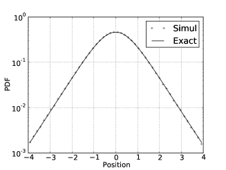
(a) Cont/Tankov

(b) AIMH

(c) AISF

Figure 7: Simulated and exact NIG PDFs at $t=1$. The AIMH algorithm has heavy tails.

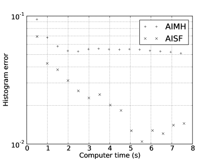
Figure 8: NIG histogram error at $t=1$, versus computer time. The AISF clearly converges faster. AIMH reaches a steady state in the convergence plot due to the error caused by the nonvanishing jump correlations.

The direct algorithm from [3] works best, as expected. We are doing this to compare AIMH and AISF, for a known case with an exact solution. The AIMH and AISF algorithms are general and can be used on any Levy process that allows a jump-diffusion approximation. This case gives us an indication of how trustworthy these methods are when applied to more exotic Levy processes for which we do not have an exact result or a simplified simulation methods as in this case.

Most sources of errors are common to both algorithms. These are related to inaccuracy in the calculation of the $\sigma$ and $\lambda$, the latter being related to the cutoff imposed on the jump domain $\Omega$. This cutoff will cause an inaccuracy in $\lambda$ since the total weight of $\Omega$ will not be calculated. Improved subdivision schemes of $\Omega$ are possible, e.g. employing coordinate transformations that transform $\Omega$ into a compact domain. We have not done this, since it unimportant for the matters we are considering.

We note that AIMH will never be completely correlation-free, and will therefore tend to produce heavy tails as is obvious in Figure 7. No such problem exists for AISF. The cutoff on $\Omega$ will naturally lead to weak tails, as seen in the plot. This can be remedied by enlarging the cutoff value, and/or treating large jumps differently.

The measurement data for convergence analysis is plotted in Figure 8, from which one readily sees that the AISF algorithm converges faster and more exactly.

6.3 Simulation of CGMY

As a second example of a pure jump infinite activity process, we turn to CGMY [2]. In this case we have no closed form expression for the distribution. We do however have the characteristic function, from which the distribution can be obtained by means of a numerical inverse Fourier transform. We have performed this calculation, and used the result as a the benchmark against which our path simulation algorithms are compared.

In this case, the Levy density is

$$\nu(x)=\left\{\begin{array}[]{ll}Ce^{-Mx}/x^{1+Y}&,x>0\\ Ce^{-G|x|}/|x|^{1+Y}&,x<0.\end{array}\right.$$ (13)

The parameter space for the CGMY model is $C,G,M>0$ and $Y<2$. By expanding the Levy density in negative powers of $x$ around the origin and keeping only the lowest order terms, we get

$$\sigma(\epsilon)\sim\epsilon^{1-Y/2},$$

so by (10), the jump-diffusion approximation is valid only for $0<Y\leq 1$. In fact, the volatility can in this case be expressed exactly in terms of the incomplete gamma function, which we will not show here.

We simulated the CGMY process with parameters $C=G=M=1$, $Y=1/2$, using $\epsilon=0.005$, and 100000 paths. In this case, the volatility for our choice of parameter values is

$$\sigma\approx 0.022.$$

Also in this case it has negligible influence on the distribution tails at $t=1$.

The results for the distribution at $t=1$ of the process is given in Figure 9, and the convergence measurements are plotted in Figure 10. The conclusions are similar to the NIG case.

(a) AIMH

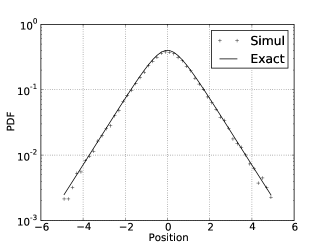
(b) AISF

Figure 9: CGMY PDF at $t=1$, simulated and exact results. Note again the heavy tails in the AIMH case.

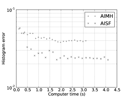
Figure 10: CGMY histogram error at $t=1$, versus computer time.

7 Conclusions

We have studied two algorithms for jump-diffusion and infinite activity pure jump process simulation via jump-diffusion approximations. Most importantly, we have studied the proposed SF algorithm based on a stochastic step function. It has some advantages over MH accept/reject algorithms. It is possible to configure it to have an arbitrarily small autocorrelation. Our simulations show that in the case of simulation of Levy processes, this algorithm can represent an improvement over the MH method that we have considered. The numerical results show an improvement in the tails of the distribution of the Levy process at a given time while at the same time converging faster. The MH algorithm will tend to give heavy tails, due to the problem of positive correlations between large jump values.

In our computer simulations, we also implemented a subdomain discretization with a corresponding adaptively improved discrete probability distribution. This method helps to reduce correlations for the MH algorithms, since the subdomains themselves are drawn without using an accept/reject algorithm. In the SF case, it improves the variate generation speed while maintaining the correlation-free nature of the method.

References

- [1] S. Asmussen and J. Rosinski, Approximations of small jumps of lévy processes with a view towards simulation, J. Appl. Probab., 38 (2001), pp. 482–493.
- [2] P. Carr, H. Geman, D. B. Madan, and M. Yor, Stochastic Volatility for Lévy Processes, 2001.
- [3] R. Cont and P. Tankov, Financial Modelling with Jump Processes, Chapman & Hall/CRC Financial Mathematics Series, 2003.
- [4] W. K. Hastings, Monte Carlo sampling methods using Markov chains and their applications, Biometrika, 57 (1970), pp. 97–109.
- [5] G. P. Lepage, New algorithm for adaptive multidimensional integration, Journal of Computational Physics, 27 (1978), pp. 192–203.
- [6] R. Merton, Option pricing when underlying stock returns are discontinuous, Journal of Financial Ecenomics, 3 (1976), pp. 125–144.
- [7] N. Metropolis, A. W. Rosenbluth, M. N. Rosenbluth, A. H. Teller, and E. Teller, Equation of state calculations by fast computing machines, The Journal of Chemical Physics, 21 (1953), pp. 1087–1092.
- [8] A. J. Walker, An efficient method for generating discrete random variables with general distributions, ACM Trans on Mathematical Software, 3 (1977), pp. 253–256.