Ultra-Narrow Faraday Rotation Filter at the Rb D₁ Line

Abstract

We present a theoretical and experimental study of the ultra-narrow bandwidth Faraday anomalous dispersion optical filter (FADOF) operating at the rubidium D₁ line ($795\text{\,}\mathrm{n}\mathrm{m}$). This atomic line gives better performance than other lines for the main FADOF figures of merit, e.g. simultaneously $71\%$ transmission, $445\text{\,}\mathrm{M}\mathrm{H}\mathrm{z}$ bandwidth and $1.2\text{\,}\mathrm{G}\mathrm{H}\mathrm{z}$ equivalent noise bandwidth.

¹ICFO-Institut de Ciencies Fotoniques, Mediterranean Technology Park, E-08860 Castelldefels (Barcelona), Spain
²Instytut Fizyki Doświadczalnej, Uniwersytet Warszawski, PL-00-681 Warszawa, Poland
³COPL, Département de Génie Physique, École Polytechnique de Montréal, C.P. 6079, Succ. Centre-ville, Montréal (Québec) H3C 3A7, Canada
⁴ICREA, Passeig Lluís Companys, 23, E-08010 Barcelona, Spain
^∗Corresponding author: morgan.mitchell@icfo.es

020.1335, 010.3640

Ultra-narrow bandwidth optical filters are key elements in laser remote sensing (LIDAR), observational astronomy, free-space communications and quantum optics. Relative to conventional interference filters, FADOFs offer high background-rejection, mechanical robustness, imaging capability and high transmission. FADOFs have been developed for several alkali atom resonances – Cs D₂ [1] and $6S_{1/2}\rightarrow 7P_{3/2}$ [2] lines, Rb D₂ line [3, 4], K (three lines) [5], Na D lines [6], and for Ca [7].

We demonstrate a FADOF on the D₁ line of Rb (wavelength $795\text{\,}\mathrm{n}\mathrm{m}$). This line, efficiently detected with Si detectors, accessible with a variety of laser technologies, and with large hyperfine splittings, is a favorite for coherent and quantum optics with warm atomic vapors. Applications include electromagnetically-induced transparency [8], stopped light [9], optical magnetometry [10, 11], laser oscillators [12], polarization squeezing [13, 14], quantum memory [15] and high-coherence heralded single photons [16, 17].

Here we show that the Rb D₁ line provides superior FADOF performance. We demonstrate a FADOF surpassing other atoms and other Rb transitions for key figures of merit, including peak transmission $T_{\rm max}$, transmission bandwidth and equivalent noise bandwidth ${\rm ENBW}={T^{-1}_{\rm max}}\int T(\nu)d\nu$, where $T(\nu)$ is the filter transmission versus frequency $\nu$ [4].

A FADOF, shown schematically in Figure 1 (inset), consists of an atomic vapor cell between two crossed polarizers. A homogeneous magnetic field along the propagation direction induces circular birefringence in the vapor. The crossed polarizers block transmission away from the absorption line, while the absorption itself blocks resonant light. Nevertheless, Faraday rotation just outside the Doppler profile can give high transmission for a narrow range of frequencies. FADOF is simple and robust, but performance depends critically on optical properties of the atomic vapor. We model these with a first-principles calculation and find excellent agreement with experiment, as shown in Figure 1.

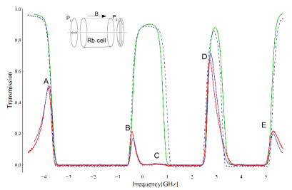
Figure 1: Absorption spectrum for Rb D₁: theory (green), experiment (black dashed). FADOF transmission spectrum: theory (blue), experiment (red). Conditions: $T=$365\text{\,}\mathrm{K}$$, $B=$4.5\text{\,}\mathrm{m}\mathrm{T}$$. Inset - FADOF setup.

Experiment

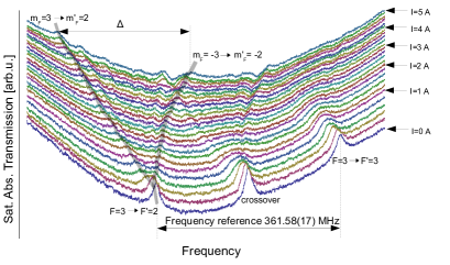
Figure 2: Saturated absorption spectra of the Doppler-broadened line (⁸⁵Rb transitions from the $F=3$ ground state) for different coil currents. Splitting $\Delta$ between Zeeman-split lines provides a precise measure of the field.

We use a rubidium cell, with anti-reflection coated windows, a $10\text{\,}\mathrm{c}\mathrm{m}$ internal path, no buffer gas or wall coatings and natural abundance rubidium (Technical Glass, Inc.). An oven and solenoidal field coil allow the cell to be maintained at constant temperature in a uniform axial field. Probe light at $795\text{\,}\mathrm{n}\mathrm{m}$ from a Littrow-configuration external-cavity diode laser (Toptica DL100) is spatially-filtered with a fiber and prepared in an adjustable linear polarization using quarter- and half-waveplates. After the cell, the beam is polarization-filtered with a linear polarizer (colorPol VIS IR) and detected with a low-noise amplified photodiode.

Saturated absorption spectroscopy was used to calibrate field strength produced by the solenoid current, as shown in Figure 2. Labeling the eigenstates by the total angular momentum quantum numbers $(F,m_{F})$, the zero-field splitting between the $(3,m)\rightarrow(2,m)^{\prime}$ and $(3,m)\rightarrow(3,m)^{\prime}$ transitions of ⁸⁵Rb provides a precise reference for the frequency scale, while the splitting $\Delta$ between $(3,3)\rightarrow(2,2)^{\prime}$ and $(3,-3)\rightarrow(2,-2)^{\prime}$ is maximally sensitive to magnetic field. Comparing the observed splittings to the first-principles model, we find the field with $\pm 0.6$ % accuracy. Absorption spectra, acquired at the same time as the FADOF spectra, are used to calibrate the frequency axis, which otherwise would be non-linear due to piezo hysteresis. These same spectra indicate the temperature with an uncertainty of $\pm$ $2\text{\,}\mathrm{K}$.

The FADOF transmission was measured under a variety of temperature and field conditions in the range T = 355–$380\text{\,}\mathrm{K}$ and B = 3.3–$6.0\text{\,}\mathrm{m}\mathrm{T}$. Typical results, taken at $4.5\text{\,}\mathrm{m}\mathrm{T}$ and $365\text{\,}\mathrm{K}$, are shown in Figure 1 and show an agreement with the model at the few-percent level. This field/temperature combination gives a single dominant peak with transmission of 70% at +$2.8\text{\,}\mathrm{G}\mathrm{H}\mathrm{z}$ relative to line center with FWHM of $445\text{\,}\mathrm{M}\mathrm{H}\mathrm{z}$. Other peaks, of transmission 49%, 17% and 20% are also present, giving an ENBW of $1.2\text{\,}\mathrm{G}\mathrm{H}\mathrm{z}$, considerably better than reported for other atoms. As shown in Table 1, the Rb D₁ FADOF also achieves narrower bandwidths than other transitions and can achieve transmission up to 92% consistent with ultra-low ENBW.

Table 1: Comparison of reported FADOF transmission for different atoms and wavelengths. T_max: peak transmission. B_T: full-width at half-maximum bandwidth of main transmission peak. B_N: Equivalent-noise bandwidth (ENBW). - value not reported. Reference [5] also shows a K $770\text{\,}\mathrm{n}\mathrm{m}$ FADOF curve very similar to K $766\text{\,}\mathrm{n}\mathrm{m}$.

Atom	$\lambda$[nm]	Ref.	Tmax	BT[GHz]	BN[GHz]
K	405	[5]	0.93	1.2	6
Ca	423	[7]	0.55	1.5	-
Cs	455	[2]	0.96	0.9	3.3
Na	589	[6]	0.85	1.9	5.1
Na	590	[6]	0.37	10.5	8.3
K	766	[5]	0.96	0.9	5
Rb	780	[4]	0.93	1.3	4.7
Cs	852	[1]	0.90	0.6	-
T[K]	B[mT]
353	18.0		0.92	0.48	2.1
378	5.9		0.91	1.10	2.7
365	4.5		0.71	0.45	1.2
345	2.0		0.04	0.32	0.8

The superior performance of the Rb D₁ line appears to be a fortunate accident of the hyperfine splittings. For either pure ⁸⁵Rb or pure ⁸⁷Rb, the FADOF transmission at these field strengths shows four peaks, with the strongest ones at the extremes of the spectrum and with long tails. The strong ⁸⁷Rb peaks are visible as peak A and E of Figure 1. The strong ⁸⁵Rb peaks include one at $-2.5\text{\,}\mathrm{G}\mathrm{H}\mathrm{z}$, completely obscured by the ⁸⁷Rb absorption, and the peak D. The long tail of peak D is blocked by absorption from the ⁸⁷Rb $1\rightarrow 1$ transition, improving ENBW.

Conclusions

We have demonstrated a Faraday anomalous dispersion optical filter (FADOF) operating at the rubidium D1 line. The filter gives high transmission and narrow bandwidth, with typical numbers being 0.5 GHz bandwidth, maximum transmission of 0.7 and equivalent-noise bandwidth of $1.2\text{\,}\mathrm{G}\mathrm{H}\mathrm{z}$, surpassing similar filters using other atoms and/or other optical transitions. The spectrum can be optimized for different figures of merit by adjusting the temperature and magnetic field conditions of the atomic vapor. A theoretical model shows excellent agreement with experimental results. The simplicity and high noise-rejection may make the new filter attractive for LIDAR and free-space communications and introduces FADOF for the D₁ line, widely preferred for coherent and quantum optical applications.

Appendix: FADOF spectra calculation

For completeness, we present the full theoretical model of the Rb D₁ FADOF. A Mathematica notebook to perform the calculations is available with this document at http://arxiv.org/.

The Rb D transitions connect the $5^{2}S_{J=1/2}$ ground states to the $5^{2}P_{J=1/2}$ (D₁) and $5^{2}P_{J=3/2}$ (D₂) excited states. Within each manifold, the Zeeman/hyperfine structure is determined by the Hamiltonian

$$\hat{H} = E_{\rm F}+\hat{H}_{{\rm Ze}}+\hat{H}_{\rm HF}$$ (1)

$$\hat{H}_{{\rm Ze}} = -g_{J}\mu_{B}(\boldsymbol{B}\cdot\boldsymbol{\mathrm{\hat{J})}}\otimes\mathbb{\mathrm{\mathbb{I}}}_{2I+1}$$ (2)

$$-g_{I}\mu_{B}\mathbb{\mathrm{\mathbb{I}}}_{2J+1}\otimes(\boldsymbol{B}\cdot\mathrm{\mathbf{\hat{I}})}$$

$$\hat{H}_{\rm HF} = A_{\rm HF}\hat{D}_{\rm HF}+B_{\rm HF}\hat{Q}_{\rm HF}$$ (3)

$$\hat{D}_{\rm HF} = \boldsymbol{\mathrm{\hat{J}\circ}}\hat{\mathbf{\boldsymbol{I}}}$$ (4)

$$\hat{Q}_{\rm HF} = \left\{\begin{array}[]{ll}\frac{3(\boldsymbol{\mathrm{\hat{J}\circ}}\hat{\mathbf{\boldsymbol{I}}})^{2}+\frac{3}{2}\boldsymbol{\mathrm{\hat{J}\circ}}\hat{\mathbf{\boldsymbol{I}}}-I(I+1)J(J+1)}{2I(2I-1)J(2J-1)}&J>1/2\\ 0&{\rm otherwise}\end{array}\right.$$ (7)

where $E_{\rm F}$ is the level energy including the fine structure contribution, $A_{\rm HF}$ and $B_{\rm HF}$ are magnetic dipole and quadrupole energies, $\bf\hat{J}$ and $\bf\hat{I}$ are vector operators representing the total electronic and nuclear angular momenta, respectively, $\boldsymbol{\mathrm{\hat{J}\circ}}\hat{\mathbf{\boldsymbol{I}}}\equiv\hat{J}_{x}\otimes\hat{I}_{x}+\hat{J}_{y}\otimes\hat{I}_{y}+\hat{J}_{z}\otimes\hat{I}_{z}$, $g_{J}$ and $g_{I}$ are total electronic and nuclear gyromagnetic factors, respectively, $\mathbb{\mathrm{\mathbb{I}}}_{n}$ is the $n$-dimensional identity matrix and $\mu_{B}$ is the Bohr magneton. All constants are taken from Steck [18, 19].

The transition electric dipole operator $\bf\hat{D}$, with circular components $\hat{D}_{q}$, $q=0,\pm 1$, is given by

$$D^{J,m_{J},J^{\prime},m_{J}^{\prime}}_{q} = \left\langle J||\hat{D}||J^{\prime}\right\rangle(-1)^{J^{\prime}-1+m_{J}}$$ (10)

$$\times\sqrt{2J+1}\left(\begin{array}[]{ccc}J^{\prime}&1&J\\ m^{\prime}_{J}&q&m_{J}\end{array}\right)$$

where last expression $(:::)$ is the Wigner 3-j symbol. The reduced dipole moment $\left\langle J||\hat{D}||J^{\prime}\right\rangle$ for each isotope is given by Steck [18, 19].

For ⁸⁵Rb ($I=5/2$) or ⁸⁷Rb ($I=3/2$), and for the ground and excited state manifolds, the Hamiltonian of Eq. (1) is diagonalized to find transition frequencies $\omega_{ba}\equiv\omega_{b}-\omega_{a}$ and their corresponding dipole matrix elements $D^{ab}_{q}=\left<a\right|\hat{D}_{q}\left|b\right>$, between all pairs of ground and excited states $\left|a\right>,\left|b\right>$. The (linear) electric susceptibility tensor $\boldsymbol{\chi}$ is diagonal in the circular ($q=\pm 1$) basis, and we compute its diagonal entries (in S.I. units) as

$$\chi_{qq}(\omega) = \sum_{{Z}\in\{85,87\}}\frac{N_{{Z}}(T)}{\epsilon_{0}\hbar}\sum_{a,b}|D_{q}^{ab}|^{2}(\rho_{bb}-\rho_{aa})$$ (11)

$$\times V(\sigma,\frac{\Gamma}{2},\omega_{ba}-\omega)$$

where $N_{{Z}}(T)$ is the atomic number density for the isotope ${Z}$, $T$ is the temperature, $\varepsilon_{0}$ is the vacuum permittivity, $\rho\propto\exp[-H/(k_{\rm B}T)]$ is the atomic density matrix and $k_{\rm B}$ is the Boltzmann constant. The Voigt profile is

$$V(\sigma,\frac{\Gamma}{2},\omega_{ba}-\omega) = i\sqrt{\frac{\pi}{2\sigma^{2}}}e^{x^{2}}\textrm{Erfc}(x),$$ (12)

where $\rm Erfc$ is the complementary error function, $x\equiv[{\frac{\Gamma}{2}+i(\omega_{ba}-\omega)}]/({\sqrt{2}\sigma})$, and $\sigma=\omega_{ba}\sqrt{{k_{\rm B}T}/({M_{Z}c^{2}})}$. Atomic masses $M_{Z}$ and natural linewidths $\Gamma$ are given in [18, 19].

Atom number density is calculated as $N_{{Z}}(T)=c_{{Z}}N_{{Z}}^{(\rm pure)}(T)$, where $c_{{Z}}$ are the relative abundances, the single-isotope densities are $N_{{Z}}^{(\rm pure)}(T)=P_{{Z}}(T)/(RT)$ where $R$ is the ideal-gas constant and the single-isotope vapor pressures $P_{{Z}}(T)$ are from Steck [18, 19]. We assume natural abundance $c_{{85}}=0.7217$ and $c_{{87}}=0.2783$.

The transmission of the filter is

$$T=|E_{\rm det}^{\dagger}\cdot M_{\rm cell}\cdot E_{\rm in}|^{2},$$ (13)

where $E_{\rm in}=(1,1)^{T}/\sqrt{2}$ is the Jones vector, in the circular left/right basis, of the linearly polarized input, $M_{\rm cell}={\rm diag}(\exp[in_{L}kL],\exp[in_{R}kL])$ is the transmission matrix of the cell, $n_{q}=\sqrt{1+\chi_{qq}}$, $E_{\rm det}=(1,-1)/\sqrt{2}$ is the Jones vector of the detected polarization, $k=\omega_{\rm laser}/c$ and $L$ is the cell internal path length.

References

- [1] J. Menders, K. Benson, S. H. Bloom, C. S. Liu, and E. Korevaar, Opt. Lett. 16, 846 (1991).
- [2] T. Yin, B. Shay, IEEE Photonics Technology Letters 4, 488 (1992).
- [3] B. Yin, L. S. Alvarez, and T. M. Shay, “The rb 780-nanometer faraday anomalous dispersion optical filter: Theory and experiment”, Tech. rep., Jet Propulsion Laboratory (1994).
- [4] D. J. Dick and T. M. Shay, Opt. Lett. 16, 867 (1991).
- [5] B. Yin and T. Shay, Optics Communications 94, 30 (1992).
- [6] H. Chen, C. Y. She, P. Searcy, and E. Korevaar, Opt. Lett. 18, 1019 (1993).
- [7] Y. C. Chan and J. Gelbwachs, IEEE Journal of Quantum Electronics 29, 2379 (1993).
- [8] X. Yang, S. Li, C. Zhang, and H. Wang, J. Opt. Soc. Am. B 26, 1423 (2009).
- [9] R. M. Camacho, P. K. Vudyasetu, and J. C. Howell, Nat Photon 3, 103 (2009).
- [10] V. I. Yudin, A. V. Taichenachev, Y. O. Dudin, V. L. Velichansky, A. S. Zibrov, and S. A. Zibrov, Phys. Rev. A 82, 033807 (2010).
- [11] F. Wolfgramm, A. Cerè, F. A. Beduini, A. Predojević, M. Koschorreck, and M. W. Mitchell, Phys. Rev. Lett. 105, 053601 (2010).
- [12] W. F. Krupke, R. J. Beach, V. K. Kanz, and S. A. Payne, Opt. Lett. 28, 2336 (2003).
- [13] J. Ries, B. Brezger, and A. I. Lvovsky, Phys. Rev. A 68, 025801 (2003).
- [14] I. H. Agha, G. Messin, and P. Grangier, Opt. Express 18, 4198 (2010).
- [15] M. Hosseini, G. Campbell, B. M. Sparkes, P. K. Lam, and B. C. Buchler, Nat Phys advance online publication, (2011).
- [16] A. Cerè, V. Parigi, M. Abad, F. Wolfgramm, A. Predojević, and M. W. Mitchell, Opt. Lett. 34, 1012 (2009).
- [17] F. Wolfgramm, Y. A. de Icaza Astiz, F. A. Beduini, A. Cerè, and M. W. Mitchell, Phys. Rev. Lett. 106, 053602 (2011).
- [18] D. A. Steck, “Rubidium 85 d line data, revision 2.1.4”, available online at http://steck.us/alkalidata (23 December 2010).
- [19] D. A. Steck, “Rubidium 87 d line data, revision 2.1.4”, available online at http://steck.us/alkalidata (23 December 2010).