Statistics of cross sections of Voronoi tessellations

Abstract

In this paper we investigate relationships between the volumes of cells of three-dimensional Voronoi tessellations and the lengths and areas of sections obtained by intersecting the tessellation with a randomly oriented plane. Here, in order to obtain analytical results, Voronoi cells are approximated to spheres. First, the probability density function for the lengths of the radii of the sections is derived and it is shown that it is related to the Meijer $G$-function; its properties are discussed and comparisons are made with the numerical results. Next the probability density function for the areas of cross sections is computed and compared with the results of numerical simulations.

I Introduction

Three-dimensional Voronoi tessellations provide a powerful method of subdividing space in random partitions and have been used in a variety of fields such as computational geometry and numerical computing (see for instance Du and Wang (2005) and the references therein), data analysis and compression Kanungo et al. (2002), geology Blower et al. (2002), and molecular biology Poupon (2004); Dupuis et al. (2011). However, in many experimental conditions it is not possible to directly observe the cells themselves, just their planar or linear sections: thus it is of interest to study the relationships between the geometric properties of three-dimensional structures and their lower dimensional sections Okabe et al. (1992).

A basic result has been proved in Chiu et al. (1996): the intersection between an arbitrary but fixed plane and a spatial Voronoi tessellation is not necessarily a planar Voronoi tessellation. An analysis of some aspects of the sections of Voronoi diagrams can be found in Okabe et al. (1992). However, a far as we know, no analytical formulas have been derived for the distributions of the lengths and areas of the planar sections: this is precisely the aim of this note.

Following  Okabe et al. (1992), a three-dimensional Voronoi diagram will be denoted by $\mathcal{V}$, and section of dimensionality $s$ will be denoted by ${\mathcal{V}}(s,3)$.

In the next section, some probability density functions used to fit empirical, or simulated, distributions of Voronoi cells size will be reviewed and in Section III, results will be presented on the distribution of the lengths and areas of $\mathcal{V}(2,3)$.

II Probability density functions of Voronoi tessellations

A Voronoi tessellation is said to be a Poisson Voronoi diagram (PVD), denoted by ${\mathcal{V}}_{p}$, if the centers generating the cells are uniformly distributed. In the case of one-dimensional PVD, with average linear density $\lambda$, a rigorous result can be derived, namely that the distribution of the lengths of the segments has the probability density function

$$p(l)=4\lambda^{2}l\exp{(-2\lambda l)},$$ (1)

or, by using the standardized variable $x=l/<l>=\lambda l$ Kiang (1966),

$$p(x)=4x\exp{(-2x)}.$$ (2)

No analytical results are known for the distribution of the sizes of Voronoi diagrams in 2D or 3D; typically distributions of the surfaces or volumes of the Voronoi cells are fitted with a $3$-parameter generalized gamma PDF of the standardized variable $x$, Hinde and Miles (1980), Tanemura (2003),

$$g(x;a,b,c)=c\frac{b^{a/c}}{\Gamma(a/c)}x^{a-1}\exp{(-bx^{c})}\quad.$$ (3)

It should be noted that from $g(x;a,b,c)$ other, simpler, probability density functions can be derived, that have been also used to model empirical distributions of PVD: for instance, by setting $a=b$ and $c=1$, the one-parameter distribution proposed in Kiang (1966) results in

$$h(x;b)=\frac{b^{b}}{\Gamma(b)}(x)^{b-1}\exp(-bx),$$ (4)

with variance

$$\sigma_{h}^{2}=\frac{1}{c}.$$ (5)

Similarly, set $a=b=({3d+1})/2$, $c=1$, where $d$ is the dimensionality of the cells: Eq. (3) then becomes

$$p(x;d)=\left(\frac{3d+1}{2}\right)^{\frac{3d+1}{2}}x^{\frac{3d-1}{2}}\exp{(-(3d+1)x/2)},\quad.$$ (6)

with variance

$$\sigma_{p}^{2}=\frac{2}{3d+1}.$$ (7)

This PDF has been shown to give a good fit for Poisson Voronoi diagrams Ferenc and Néda (2007), even though it has no free parameters: it will be used in the following to model distributions of the volumes of three-dimensional Voronoi tessellations.

III Sections

Consider a three-dimensional Poisson Voronoi diagram and suppose it intersects a randomly oriented plane $\gamma$: the resulting cross sections are polygons, as in the example shown in Fig. 1.

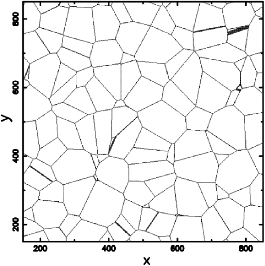
Figure 1: Planar cross sections of a three-dimensional Voronoi tessellation.

In order to obtain analytical results for the distributions of the lengths and areas of ${\mathcal{V}}_{p}(2,3)$, some simplifying hypothesis is needed: here the cells will be supposed to be spheres. This is, admittedly, a rather rough approximation, but, on the other hand, it makes all cuts of the same simple shape, i.e. circles, irrespective of the orientation of the cutting plane. As shown in the sequel, this approximation allows of deriving an analytical form for the distributions of the radii lengths and the areas of cell sections.

Let $f_{V}(V)$ be the probability density function for the cell volumes, then the PDF $f_{R}(R)$ for the lengths of their radii is given by

$$f_{R}\left(R\right)=f_{V}\left(\frac{4}{3}\pi R^{3}\right)4\pi R^{2}.$$ (8)

The use of Eq. (8) and of the standardized PDF (6), with $d=3$, leads to

$$f_{R}(R)={\frac{4\cdot 10^{5}}{243}}\,{\pi}^{5}{R}^{14}\exp\left(-{\frac{20}{3}}\,\pi\,{R}^{3}\right).$$ (9)

A plot of $f_{R}$ is shown in Fig. 2.

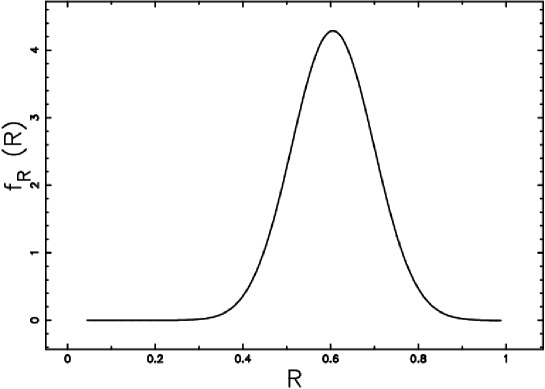
Figure 2: The PDF $f_{R}$ as a function of $R$.

Consider now the intersection of a sphere of radius $R$ with a randomly oriented plane: the PDF of $r$, the length of the radius of the resulting circle, is Blower et al. (2002)

$$\pi_{c}(r)=\int_{r}^{\infty}f_{R}(R)\frac{1}{R}\frac{r}{\sqrt{R^{2}-r^{2}}}dR.$$ (10)

The probability of a plane’s intersecting a sphere is proportional to $R$ Blower et al. (2002) so, in conclusion, the PDF of $r$ can be written as

$$f_{r}(r)=\alpha\int_{r}^{\infty}f_{R}(R)\frac{r}{\sqrt{R^{2}-r^{2}}}dR.$$ (11)

Insertion of Eq. (9) into (11) results in the formula

$$f_{r}(r)=\alpha{\frac{4\cdot 10^{5}}{243}}\,{\pi}^{5}\int_{r}^{\infty}{R}^{14}\exp\left(-{\frac{20}{3}}\,\pi\,{R}^{3}\right)\frac{r}{\sqrt{R^{2}-r^{2}}}dR.$$ (12)

The integral (12) can be solved by making use of a computer algebra system such as MAPLE: the result is

$$f_{r}(r)=2/3\,{\alpha}\,\sqrt[6]{3}\sqrt[3]{10}\sqrt[3]{\pi}rG^{4,1}_{3,5}\left({\frac{100}{9}}\,{\pi}^{2}{r}^{6}\,\Big{|}\,^{5/6,1/6,1/2}_{7/3,2/3,1/3,0,{\frac{17}{6}}}\right),$$ (13)

where $G$ is the Mejier $G$-function Meijer (1936, 1941); Olver et al. (2010); the numerical value of $\alpha$, obtained via normalization of $f_{r}$ is $\alpha=1.649$. A plot of $f_{r}$ is shown in Fig. 3.

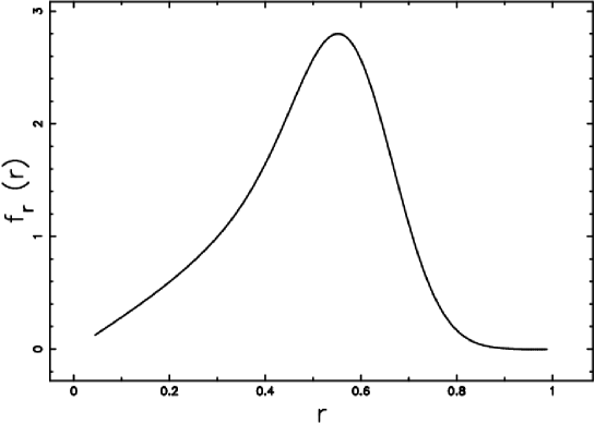
Figure 3: The probability density function $f_{r}$ as a function of $r$.

The Meijer $G$ function is very complicated and Eq. (13) does not lend itself to ready interpretation; moreover, at the best of our knowledge, it allows no simple approximations ( see Luke, J. L. (1969)).

However, some insight into the form of $f_{r}$ can be gained by considering Taylor expansions. In the interval $[0,0.1]$ $f_{r}$ is linear, $f_{r}(r)\approx 2.78r$, while for $r$ close to $1$, in the interval $[0.9,1]$, it is well approximated by a quadratic polynomial:

$$f_{r}(r)\approx-0.006\,\left(r-1\right)+0.136\,\left(r-1\right)^{2}.$$ (14)

The mode occurs in the interval $[0.5,0.6]$, where a close approximation of $f_{r}$ is given by

$$f_{r}(r)\approx 2.48+0.58\,r-95.528\,\left(r-0.55\right)^{2}-202.18\,\left(r-0.55\right)^{3}+1901.87\,\left(r-0.55\right)^{4};$$ (15)

from this formula the mode $m$ can be easily computed: $m=0.553$.

The mean and variance of $f_{r}$ are $\left<r\right>=0.487$ and $\sigma^{2}_{r}=0.025$, respectively; $f_{r}$ is moderately left skewed (skewness $\gamma_{r}=-0.522$) and is slightly platykurtic (excess kurtosis $k_{r}=-0.111$). For comparison, note that $f_{R}$ is more symmetric ( skewness $\gamma_{R}=0.014$) and has fatter tails (excess kurtosis $k_{R}=-0.005$).

The distribution function $F_{r}$ is

$$F_{r}(r)={\frac{1}{90}}\,{\alpha}\,{3}^{5/6}{10}^{2/3}G^{4,2}_{4,6}\left({\frac{100}{9}}\,{\pi}^{2}{r}^{6}\,\Big{|}\,^{1,7/6,1/2,5/6}_{8/3,1,2/3,1/3,{\frac{19}{6}},0}\right){\frac{1}{\sqrt[3]{\pi}}}.$$ (16)

The PDF $f_{A}$ of the areas of ${\mathcal{V}}_{p}(2,3)$ can be obtained from $f_{r}$ by means of the transformation

$$f_{A}(A)=f_{r}\left(\left(\frac{A}{\pi}\right)^{1/2}\right)\frac{\pi^{-1/2}}{2}{A}^{-1/2},$$ (17)

that is,

$$f_{A}(A)=0.549\,\sqrt[6]{3}\sqrt[3]{10}G^{4,1}_{3,5}\left({\frac{100}{9}}\,{\frac{{A}^{3}}{\pi}}\,\Big{|}\,^{5/6,1/6,1/2}_{7/3,2/3,1/3,0,{\frac{17}{6}}}\right){\pi}^{-2/3}\quad.$$ (18)

Since, for $r$ close to $0$, $f_{r}(r)\sim r$ from Eq. (17) it follows that $f_{A}(0)\neq 0$ and this result has been also verified by numerical simulations we have carried out (see also Okabe et al. (1992) for a further example). Indeed it is easy to verify that $f_{A}(0)=0.443$. Fig. 4 shows the graph of $f_{A}$.

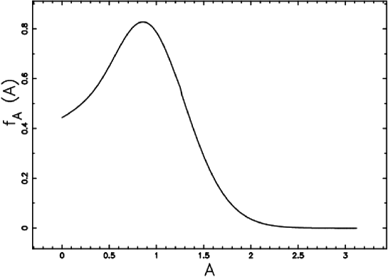
Figure 4: The PDF $f_{A}$ as a function of $A$.

The mode of $f_{A}$ is $m_{A}=0.858$, its mean and variance are $\left<A\right>=0.824$ and $\sigma^{2}_{A}=0.204$, respectively; $f_{A}$ is approximately symmetric (skewness $\gamma_{A}=0.278$) and its excess kurtosis is $k_{A}=-0.337$, indicating that the transformation from $f_{r}$ to $f_{A}$ yields a PDF with a lower and broader peak and with shorter and thinner tails.

The distribution function $F_{A}$ is given by

$$F_{A}=0.018\,{3}^{5/6}{10}^{2/3}G^{4,2}_{4,6}\left({\frac{100}{9}}\,{\frac{{A}^{3}}{\pi}}\,\Big{|}\,^{1,7/6,1/2,5/6}_{8/3,1,2/3,1/3,{\frac{19}{6}},0}\right){\frac{1}{\sqrt[3]{\pi}}}\quad;$$ (19)

A comparison has been carried out between the distribution functions $F_{r}$, $F_{A}$, as as given by Eq. (16), (19) respectively, and the results of a numerical simulation, performed as follows: starting from $300000$ $3$-dimensional cells $100168$ irregular polygons were obtained by adding together results of cuts by $41$ triples of mutually perpendicular planes.

The area of the irregular polygons has been obtained with the algorithm described in Zaninetti (1991): briefly, each cut defines a two-dimensional grid and the polygons areas we measured by counting the number of points of the grid belonging to a given cell.

As concerns the linear dimension, in our approximation the two-dimensional cells were considered circles and thus, for consistency, the radius $r$ of an irregular polygon was defined as

$$r=\left(\frac{A}{\pi}\right)^{1/2},$$ (20)

that is $r$ is the radius of a circle with the same area of the polygon, $A$. The empirical distribution of radii is shown in Fig. 5 together with the graph of $F_{r}$: the maximum distance between the empirical and analytical curves is $d_{max}=0.044$.

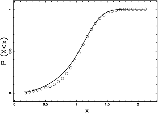
Figure 5: Comparison between theoretical distribution (continuous line) and data (empty circles) for the distribution of radii $r$ of 2D cells which result from an intersection with a plane. The maximum distance between the two curves is $d_{max}=0.044$ .

Likewise a comparison between $F_{A}$ and the simulation is shown in Fig. 6; in this case $d_{max}=0.039$.

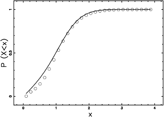
Figure 6: Comparison between data (empty circles) and theoretical curve (continuous line) of the distribution of areas. The maximum distance between the two curves is $d_{max}=0.039$.

IV Conclusions

In this paper analytical formulas have been provided which model the distributions of the lengths and areas of the planar sections of three-dimensional Poisson Voronoi diagrams: in particular, it has been shown that they are related to the Meier $G$ function.

This finding is consistent with the analytical results presented in Springer and Thompson (1970), where it is proved that nonlinear combinations of gamma variables, such as products or quotients, have distributions proportional, or closely related, to the Meijer $G$ distribution.

The analytical distributions $F_{r}$ and $F_{A}$ been compared with results of numerical simulations: in evaluating the differences between analytical and empirical distributions it must be kept in mind that the cells were approximated as spheres and that the distributions used here have no free parameters that can be adjusted to optimize the fit. The results obtained here may be useful for applications in stereology in that they allow of predicting the distributions of linear and planar measures of sections, given an arrangement of three-dimensional cells. This method can also have application to astrophysics, namely in the analysis of the spatial distributions of the voids between galaxies, that are experimentally measured as two-dimensional slices Pan et al. (2011) and that can be identified with two-dimensional cuts of a three-dimensional structure. For instance, the distribution of the radius between galaxies of the Sloan Digital Sky Survey Data Release 7 (SDSS DR7) has been reported in Pan et al. (2011); this catalog contains 1054 radii $r_{e}$ of voids. To compare these experimental data with the results obtained here one should know the values of $R_{e}$, the radii of voids in three dimensions; however by making use of standardized variables $x=r/{\langle r\rangle}$, $x_{e}=r_{e}/{\langle r_{e}\rangle}$ one obtains for the standard deviation based on observations $\sigma_{x_{e}}=0.26$, close to the theoretical value, $\sigma_{x}=0.32$. Finally, the $2D$ cuts presented in this paper may be related to Laguerre decompositions (weighted Voronoi decomposition) Telley (1989); Telley et al. (1996); Xue et al. (1997), with a weighting factor depending on the distance between the between cells and the cutting plane.

References

- Du and Wang (2005) Q. Du and D. Wang, SIAM J. Sci. Comput. 26, 737 (2005).
- Kanungo et al. (2002) T. Kanungo, D. M. Mount, N. S. Netanyahu, C. D. Piatko, R. Silverman, and A. Y. Wu, IEEE Trans. Pattern Analysis and Machine Intelligence 24, 881 (2002).
- Blower et al. (2002) J. Blower, J. Keating, H. Mader, and J. Phillips, Journal of Volcanology and Geothermal Research 120, 1 (2002), ISSN 0377-0273.
- Poupon (2004) A. Poupon, Current Opinion in Structural Biology 14, 233 (2004).
- Dupuis et al. (2011) F. Dupuis, J.-F. Sadoc, R. Jullien, B. Angelov, and J.-P. Mornon, Bioinformatics 21, 1715 (2011).
- Okabe et al. (1992) A. Okabe, B. Boots, and K. Sugihara, Spatial tessellations. Concepts and Applications of Voronoi diagrams (Wiley, Chichester, New York, 1992).
- Chiu et al. (1996) S. N. Chiu, R. V. D. Weygaert, and D. Stoyan, Advances in Applied Probability 28, 356 (1996).
- Kiang (1966) T. Kiang, Z. Astrophys. 64, 433 (1966).
- Hinde and Miles (1980) A. L. Hinde and R. Miles, J. Stat. Comput. Simul. 10, 205 (1980).
- Tanemura (2003) M. Tanemura, Forma 18, 221 (2003).
- Ferenc and Néda (2007) J.-S. Ferenc and Z. Néda, Phys. A 385, 518 (2007).
- Meijer (1936) C. Meijer, Nieuw Arch. Wiskd. 18, 10 (1936).
- Meijer (1941) C. Meijer, Proc. Akad. Wet. Amsterdam 44, 1062 (1941).
- Olver et al. (2010) F. W. J. e. Olver, D. W. e. Lozier, R. F. e. Boisvert, and C. W. e. Clark, NIST handbook of mathematical functions. (Cambridge University Press. , Cambridge, 2010).
- Luke, J. L. (1969) Luke, J. L., The special functions and their approximations. Vol. I, II. (Academic Press, New-York, 1969).
- Zaninetti (1991) L. Zaninetti, Journal of Computational Physics 97, 559 (1991).
- Springer and Thompson (1970) M. Springer and W. Thompson, SIAM J. Appl. Math. 18, 721 (1970).
- Pan et al. (2011) D. C. Pan, M. S. Vogeley, F. Hoyle, Y.-Y. Choi, and C. Park, ArXiv e-prints:1103.4156 (2011), eprint 1103.4156.
- Telley (1989) H. Telley, Ph.D. thesis, EPFL no 780, Lausanne (1989).
- Telley et al. (1996) H. Telley, T. Liebling, and A. Mocellin, Philosophical Magazine B-Physics of Condensed Matter Statistical Mechanics Electronic Optical and Magnetic Properties 73, 395 (1996).
- Xue et al. (1997) X. Xue, F. Righetti, H. Telley, T. Liebling, and A. Mocellin, Philosophical Magazine B-Physics of Condensed Matter Statistical Mechanics Electronic Optical and Magnetic Properties 75, 567 (1997).