Probing spectral properties of radio-quiet quasars searched for optical microvariability-II

Abstract

In the context of AGN unification scheme rapid variability properties play an important role in understanding any intrinsic differences between sources in different classes. In this respect any clue based on spectral properties will be very useful toward understanding the mechanisms responsible for the origin of rapid small scale optical variations, or microvariability. Here we have added spectra of 46 radio-quiet quasars (RQQSOs) and Seyfert 1 galaxies to those of our previous sample of 37 such objects, all of which had been previously searched for microvariability. We took new optical spectra of 33 objects and obtained 13 others from the literature. Their H$\beta$ and Mg ii emission lines were carefully fit to determine line widths (FWHM) as well as equivalent widths (EW) due to the broad emission line components. The line widths were used to estimate black hole masses and Eddington ratios, $\ell$. Both EW and FWHM are anticorrelated with $\ell$. Nearly all trends were in agreement with our previous work, although the tendency for sources exhibiting microvariability to be of lower luminosity was not confirmed. Most importantly, this whole sample of EW distributions provides no evidence for the hypothesis that a weak jet component in the radio quiet AGNs is responsible for their microvariability.

1 Introduction

Rapid small scale optical variations, or intra-night microvariability is a well known characteristic of Active Galactic Nuclei (AGNs) but the processes causing the bulk of these microvariations is still a matter of debate. The variability mechanisms in the radio-loud objects are widely believed to be connected to conditions in the relativistic jet. However, it is still unclear if in the radio-quiet objects the nature of intra-night variability is different, or whether the faint, variable jet is also a dominant component for them. Czerny et al. (2008) have tried to understand the microvariation mechanism within the framework of following scenarios: (i) fluctuations from an accretion disk (e.g., Mangalam & Wiita 1993); (ii) irradiation of an accretion disc by a variable X-ray flux (e.g., Rokaki, Collin-Souffrin & Magnan 1993; Gaskell 2006); and (iii) the presence of modestly misaligned jets in radio-quiet quasars or a “blazar component” (e.g., Gopal-Krishna et al. 2003). They concluded that the blazar component model is the most promising to give rise to intra-night optical variability.

In this blazar component scenario, spectral properties of the sources can play a crucial role in constraining the models further. For instance, if blazar components are dominating the variability of RQQSOs, then, due to the increase in the continuum produced by the jets one expects smaller equivalent widths (EW) of prominent emission lines such as H$\beta$ and Mg ii for sources with microvaraibility as compared to their average value in a sample including non-variable sources. Recently, in Chand, Wiita & Gupta (2010; hereafter Paper I), we have worked toward this goal by exploiting the optical spectra available from the Sloan Digital Sky Survey, Data Release 7 (SDSS DR-7; Abazajian et al. 2009). We carried out careful spectral modeling of the H$\beta$ and Mg ii emission line regions for RQQSO and Seyfert 1 samples already searched for microvariability (hereafter referred to collectively as RQQSOs). In Paper I, we first investigated any effect of key spectral parameters (e.g., EW and FWHM) on the microvariability of RQQSOs. Second, we estimated other relevant AGN parameters such as the black hole mass, M_bh and Eddington ratios. To do this, their H$\beta$ and Mg ii emission lines were carefully fit to determine line widths (FWHM) as well as equivalent widths (EW) due to the broad emission line components. The line widths were used to estimate black hole masses and Eddington ratios. The EW distributions did not provide evidence for the hypothesis that a weak jet component in the RQQSOs is responsible for their microvariability, and perhaps instead it may indicate that variations involving the accretion disc (e.g., Wiita 2006) are important for them. We also concluded that there may be a weak negative correlation between H$\beta$ EW and $\ell$, but there is a significant one between the Mg ii EW and $\ell$. In addition, we noted that there is a tendency for sources with detectable optical microvariability to have somewhat lower luminosities than those with no such detections (see Fig. 8 of Paper I) .

All the above tentative conclusions from our Paper I were certainly interesting; however, as we stressed there, it is very important that they should be tested by examining larger samples. The importance of a larger sample for such investigations is evident from our recent finding on the fraction of broad absorption line QSOs showing microvariability (Joshi et al. 2011). That fraction appeared to be 50 per cent based on only 6 sources, but using a larger sample of 23 sources, Joshi et al. (2011) found it to be around ten percent, similar to RQQSOs (Gupta & Joshi 2005).

Therefore, given the important implications of our above results, based on spectral analysis of 37 sources, for the origin of RQQSO microvariability, and hence to processes on the accretion disc itself, it becomes important to carry out spectral analyses of as many sources searched for microvariability as possible. The obvious source for such a sample would be the remainder of the objects from the total of 117 sources in the compilation of Carini et al. (2007) for which SDSS DR-7 spectra are not available. This forms the main motivation of this paper, in which we more than double the sample size by taking new spectra and gathering others from the literature that we then analyze. Results from this larger sample can test the validity of results found using our previous modest sample in Paper I.

The paper is organized as follows. Section 2 describes the data sample and selection criteria. Section 3 describes the observation and data reduction while Section 4 gives details of our spectral fitting procedure. In Section 5 we focus on BH mass measurements and in Section 6 we give estimates of Eddington ratios and of BH growth times. Section 7 gives a discussion and conclusions. Throughout, we have used flat cosmology with $H_{\rm 0}$=70 km s^-1 Mpc^-1, $\Omega_{\rm m}$=0.3 and $\Omega_{\rm\Lambda}$=0.7.

Table 1: New sample of radio-quiet QSOs and Seyfert galaxies from the compilation of Carini et al. (2007)

QSO Name	$\alpha_{2000}$	$\delta_{2000}$	$z_{em}$	m${}_{(band)}^{\star}$	M${}_{B}^{\star}$	Variable?	Class	Spectra
(1)	(2)	(3)	(4)	(5)	(6)	(7)	(8)	(9)
J000619.5$+$201210	00h 06m 19.5s	$+$20∘ 12′ 10′′	0.025	13.75(B)	-22.14	N	SY1.2	IGO
J002913.6$+$131603	00h 29m 13.6s	$+$13∘ 16′ 03′′	0.142	16.30(V)	-24.70	Y	SY1	IGO
J004547.3$+$041024	00h 45m 47.3s	$+$04∘ 10′ 24′′	0.385	15.88(B)	-26.00	N	BALQSO	IGO
J005334.9$+$124136	00h 53m 34.9s	$+$12∘ 41′ 36′′	0.058	14.39(B)	-24.43	N	SY1	IGO
J005452.1$+$252538	00h 54m 52.1s	$+$25∘ 25′ 38′′	0.154	15.42(B)	-24.40	N	SY1	IGO
J011354.5$+$390744	01h 13m 54.5s	$+$39∘ 07′ 44′′	0.234	16.70(B)	-24.10	N	SY1	IGO
J012240.6$+$231015	01h 22m 40.6s	$+$23∘ 10′ 15′′	0.052	15.41(B)	-22.12	N	SY1	IGO
J051611.4$-$000859	05h 16m 11.4s	$-$00∘ 08′ 59′′	0.032	14.10(B)	-25.20	Y	SY1	IGO
J051633.4$-$002713	05h 16m 33.4s	$-$00∘ 27′ 13′′	0.292	16.26(B)	-25.10	N	SY1.2	IGO
J055453.6$+$462622	05h 54m 53.6s	$+$46∘ 26′ 22′′	0.020	15.00(B)	-22.60	N	SY1	IGO
J071415.1$+$454156	07h 14m 15.1s	$+$45∘ 41′ 56′′	0.055	14.90(B)	-29.60	N	SY1.5	IGO
J073657.0$+$584613	07h 36m 57.0s	$+$58∘ 46′ 13′′	0.039	15.29(B)	-21.80	N	SY1.5	IGO
J084742.4$+$344504	08h 47m 42.4s	$+$34∘ 45′ 04′′	0.064	14.00(B)	-23.95	Y	SY1	IGO
J092512.9$+$521711	09h 25m 12.9s	$+$52∘ 17′ 11′′	0.035	15.62(B)	-21.00	Y	SY1	SDSS
J092603.3$+$124404	09h 26m 03.3s	$+$12∘ 44′ 04′′	0.029	14.93(B)	-21.27	N	SY1.2	SDSS
J095652.4$+$411522	09h 56m 52.4s	$+$41∘ 15′ 22′′	0.234	15.05(B)	-25.73	N	SY1	IGO
J101420.7$-$041840	10h 14m 20.7s	$-$04∘ 18′ 40′′	0.058	15.49(B)	-22.22	N	SY1	IGO
J105143.9$+$335927	10h 51m 43.9s	$+$33∘ 59′ 27′′	0.167	15.81(B)	-24.19	N	SY1	SDSS
J110631.8$-$005252	11h 06m 31.8s	$-$00∘ 52′ 52′′	0.423	16.02(B)	-25.70	Y	QSO	IGO
J111908.7$+$211918	11h 19m 08.7s	$+$21∘ 19′ 18′′	0.176	15.17(B)	-24.96	Y	SY1	IGO
J112147.1$+$114418	11h 21m 47.1s	$+$11∘ 44′ 18′′	0.050	14.65(B)	-22.69	N	SY1.2	IGO
J112302.3$-$273004	11h 23m 02.3s	$-$27∘ 30′ 04′′	0.389	16.80(V)	-25.20	N	QSO	IGO
J112439.2$+$420145	11h 24m 39.2s	$+$42∘ 01′ 45′′	0.225	16.02(B)	-24.71	N	SY 1	SDSS
J112731.9$-$304446	11h 27m 31.9s	$-$30∘ 44′ 46′′	0.673	16.30(V)	-27.00	N	QSO	IGO
J115349.3$+$112830	11h 53m 49.3s	$+$11∘ 28′ 30′′	0.176	15.51(B)	-24.61	N	SY 1	SDSS
J120309.6$+$443153	12h 03m 09.6s	$+$44∘ 31′ 53′′	0.002	13.74(B)	-17.40	N	SY1.5	NED1
J121032.6$+$392421	12h 10m 32.6s	$+$39∘ 24′ 21′′	0.003	11.50(B)	-20.60	N	SY1.5	IGO
J125048.3$+$395139	12h 50m 48.3s	$+$39∘ 51′ 39′′	1.032	16.06(V)	-27.86	N	QSO	SDSS
J125948.8$+$342323	12h 59m 48.8s	$+$34∘ 23′ 23′′	1.375	16.79(B)	-28.00	N	QSO	SDSS
J132349.5$+$654148	13h 23m 49.5s	$+$65∘ 41′ 48′′	0.168	15.86(B)	-24.23	N	SY1	IGO
J135458.7$+$005211	13h 54m 58.7s	$+$00∘ 52′ 11′′	1.127	16.00(V)	-28.06	N	QSO	IGO
J140516.2$+$255534	14h 05m 16.2s	$+$25∘ 55′ 34′′	0.164	15.57(B)	-24.46	N	SY1	IGO
J141348.3$+$440014	14h 13m 48.3s	$+$44∘ 00′ 14′′	0.089	14.99(B)	-23.68	N	SY1	IGO
J141700.7$+$445606	14h 17m 00.7s	$+$44∘ 56′ 06′′	0.113	15.74(B)	…	N	SY1	SDSS
J142906.6$+$011706	14h 29m 06.6s	$+$01∘ 17′ 06′′	0.086	15.05(B)	-23.51	N	SY1	IGO
J144207.4$+$352623	14h 42m 07.4s	$+$35∘ 26′ 23′′	0.079	15.00(B)	-23.32	N	SY1	IGO
J153638.3$+$543333	15h 36m 38.3s	$+$54∘ 33′ 33′′	0.038	15.31(B)	-21.48	N	SY1	IGO
J155202.3$+$201402	15h 52m 02.3s	$+$20∘ 14′ 02′′	0.251	17.40(V)	-24.60	N	QSO	IGO
J162011.3$+$172428	16h 20m 11.3s	$+$17∘ 24′ 28′′	0.112	15.53(B)	…	N	SY1	IGO
J170124.8$+$514920	17h 01m 24.8s	$+$51∘ 49′ 20′′	0.292	15.43(B)	-25.78	Y	BALQSO	NED2
J175116.6$+$504539	17h 51m 16.6s	$+$50∘ 45′ 39′′	0.299	15.80(B)	-25.60	Y	QSO	IGO
J211452.6$+$060742	21h 14m 52.6s	$+$06∘ 07′ 42′′	0.466	15.52(B)	-26.70	N	QSO	IGO
J213227.8$+$100819	21h 32m 27.8s	$+$10∘ 08′ 19′′	0.062	14.62(B)	-23.20	N	QSO	NED3
J221712.2$+$141421	22h 17m 12.2s	$+$14∘ 14′ 21′′	0.065	14.98(B)	-23.04	N	QSO	NED4
J230315.6$+$085226	23h 03m 15.6s	$+$08∘ 52′ 26′′	0.016	13.00(B)	-22.10	Y	SY1.2	NED5
J230702.9$+$043257	23h 07m 02.9s	$+$04∘ 32′ 57′′	0.046	15.44(B)	-21.57	N	SY1	IGO

2 Data sample and selection criteria

From the compilation of 117 radio-quiet AGNs in Carini et al. (2007), that were often extensively searched for microvariability, Paper I analyzed 33 sources (in their total sample of 37 sources), for which SDSS DR7 spectra were available. Here we examined the rest of the the 84 sources, and using their redshifts found that among them 25 sources are such that neither their H$\beta$ nor Mg ii lines fall in the optical spectral range as they have redshifts outside the following respective ranges: $z\leq 0.65;0.43\leq z\leq 1.86$. For the remaining 59 sources we found H$\beta$ and Mg ii emission lines fall in the spectral range of 3800Å-8300Å  for 50 and 9 sources, respectively.

We have searched for the optical spectra of these 59 sources in SDSS DR8 (Aihara et al. 2011) and as well as in the NED data base. We could find SDSS DR8 spectra for 8 sources and NED spectra with desired quality (good S/N and spectral coverage that cover Mg ii or H$\beta$ line) for 5 sources as listed in Table 1.

We planned the observations of the rest of the 46 sources, using the IUCAA Faint Object Spectrograph (IFOSC) mounted on the 2-m telescope at IUCAA Girawali Observatory (IGO), near Pune, India. With IGO we could obtain the desired spectra for 33 sources. Among the remaining 13 sources: 6 were not visible from IGO, having very negative declinations; 4 (J001555.1$+$023024, J012017.2$+$213346, J220311.5$-$180143 and J194240.6$-$101925) could not be observed either due to non-visibility or lack of enough observing time; 1, namely J103206.2$+$324015, was classified as a white dwarf in NED; and the remaining 2, J082740.2$+$094208 and J154559.1$+$270630, though observed, were dropped from our analysis as they showed very poor H$\beta$ lines in their spectra.

So finally we are left with a sample of 46 sources (33 new observations, 8 from SDSS DR8 and 5 from NED); among them, 42 spectra cover H$\beta$ lines while 4 spectra cover Mg ii doublet lines. The source information is listed in Table 1. The first four columns give source name, RA(J2000), DEC(J2000) and emission redshift (z_em), while the fifth column provides the apparent magnitude in either B or V band. The sixth column provides the absolute B magnitudes and the seventh column indicate microvariability detection status; the eighth column gives a source classification from among classes such as QSO, BALQSO (Broad Absorption Line QSO), or Seyfert (Sy) galaxy type. In the last column we have given the spectral resource information.

3 Observations and Data Reduction

The new spectra were obtained for 33 sources. The observations were carried out using the IFOSC mounted on the 2 meter IGO telescope. We took long-slit spectra covering the wavelength range 3800 - 6840 Å using the GR7 grism and 5800 - 8300 Å using the GR8 grism of the IFOSC to cover the Mg ii and H$\beta$ lines, respectively, as noted in the third column of the observing log in Table 2. A slit width of either 1.^′′0 or 1.^′′5 was used, as listed in the fourth column of Table 2. Typical seeing during our observations was around 1.^′′2 to 1.^′′3. The raw CCD frames were cleaned using standard IRAF procedures. We used halogen flats for flat fielding the frames. Since at $\lambda>7000$Å simple flat fielding does not remove the fringes, therefore in case of grism GR8 the QSO was moved along the slit for two different exposures at the same position angle. We subsequently removed fringing by subtracting one frame from the other taken on the same night. The same procedure was applied to standard stars as well. We then extracted the one dimensional spectrum from individual frames using the IRAF task “doslit”. Wavelength calibration of the spectra was performed using Helium-Neon lamps. The spectrophotometric flux calibration was done using standard stars and assuming a mean extinction for the IGO site. In cases when multiple exposures were needed we coadded the flux with ${1}/{\sigma_{i}^{2}}$ weightage, where ${\sigma_{i}}$ is the error on the individual pixel. The error spectrum was computed taking into account proper error propagation during the combining process. The typical median signal-to-noise (SNR) over the spectral fitting range of our sample vary from 20-150 per pixel, as listed in last column of Table 2. Our spectral range also covers atmospheric absorption line regions but in all cases our fitting regions fall either buleward or redward of them, so we need not correct for any blending due to them in our analyses.

4 Line analysis through simultaneous spectral fitting

The H$\beta$ and Mg ii emission lines were carefully modelled by using the fitting procedure we used in Paper I. The spectra were first corrected for Galactic extinction using the extinction map of Schlegel et al. (1998) and the reddening curve of Fitzpatrick (1999). Then they were transformed into the rest frame using the redshift as determined from the peak of O iii$\lambda$5007 emission line. Limited by the complications needed to fit the continuum and the Fe ii emission, viz. (i) there are essentially no emission-line free regions where the continuum can be determined (Vanden Berk et al. 2001); (ii) the prominence of Fe ii features and their blending with the H$\beta$ and Mg ii lines; (iii) the H$\beta$ line is highly blended with the O iii$\lambda\lambda$4959,5007 lines, we have opted to carry out simultaneous fits of continuum, Fe ii emission, H$\beta$ and Mg ii and all other metal emission lines present in the spectra. For this purpose we adopted the procedure as described in detail in Paper I, which in brief is as follows.

Table 2: IGO Observation log.

QSO Name	Date of Obs	Grism	slit width	SNR
J000619.5$+$201210	2009-12-13	IFOSC7	1.5′′	82
J002913.6$+$131603	2009-12-13	IFOSC7	1.0′′	73
J004547.3$+$041024	2009-12-12	IFOSC8	1.5′′	38
J005334.9$+$124136	2009-12-13	IFOSC7	1.0′′	80
J005452.1$+$252538	2009-12-12	IFOSC7	1.5′′	40
J011354.5$+$390744	2011-01-06	IFOSC7	1.5′′	19
J012240.6$+$231015	2011-02-05	IFOSC7	1.5′′	47
J051611.4$-$000859	2011-01-06	IFOSC7	1.5′′	127
J051633.4$-$002713	2009-12-12	IFOSC8	1.5′′	43
J055453.6$+$462622	2009-12-13	IFOSC7	1.0′′	47
J071415.1$+$454156	2011-02-04	IFOSC7	1.0′′	54
J073657.0$+$584613	2011-02-05	IFOSC7	1.0′′	63
J084742.4$+$344504	2009-12-12	IFOSC7	1.5′′	92
J095652.4$+$411522	2009-12-13	IFOSC7	1.0′′	44
J101420.7$-$041840	2011-02-05	IFOSC7	1.0′′	67
J110631.8$-$005252	2011-04-01	IFOSC8	1.5′′	39
J111908.7$+$211918	2010-04-18	IFOSC7	1.0′′	32
J112147.1$+$114418	2011-02-04	IFOSC7	1.0′′	41
J112302.3$-$273004	2011-04-01	IFOSC8	1.5′′	73
J112731.9$-$304446	2010-04-19	IFOSC7	1.0′′	42
J121032.6$+$392421	2010-04-18	IFOSC7	1.0′′	21
J132349.5$+$654148	2011-02-04	IFOSC7	1.0′′	150
J135458.7$+$005211	2011-03-30	IFOSC7	1.5′′	37
J140516.2$+$255534	2011-02-04	IFOSC7	1.0′′	51
J141348.3$+$440014	2010-04-17	IFOSC7	1.0′′	40
J142906.6$+$011706	2010-04-18	IFOSC7	1.0′′	31
J144207.4$+$352623	2010-04-17	IFOSC7	1.0′′	50
J153638.3$+$543333	2010-04-17	IFOSC7	1.0′′	37
J155202.3$+$201402	2011-02-05	IFOSC7	1.0′′	23
J162011.3$+$172428	2010-04-18	IFOSC7	1.0′′	23
J175116.6$+$504539	2011-03-30	IFOSC7	1.5′′	55
J211452.6$+$060742	2009-12-12	IFOSC8	1.5′′	38
J230702.9$+$043257	2009-12-14	IFOSC7	1.0′′	20

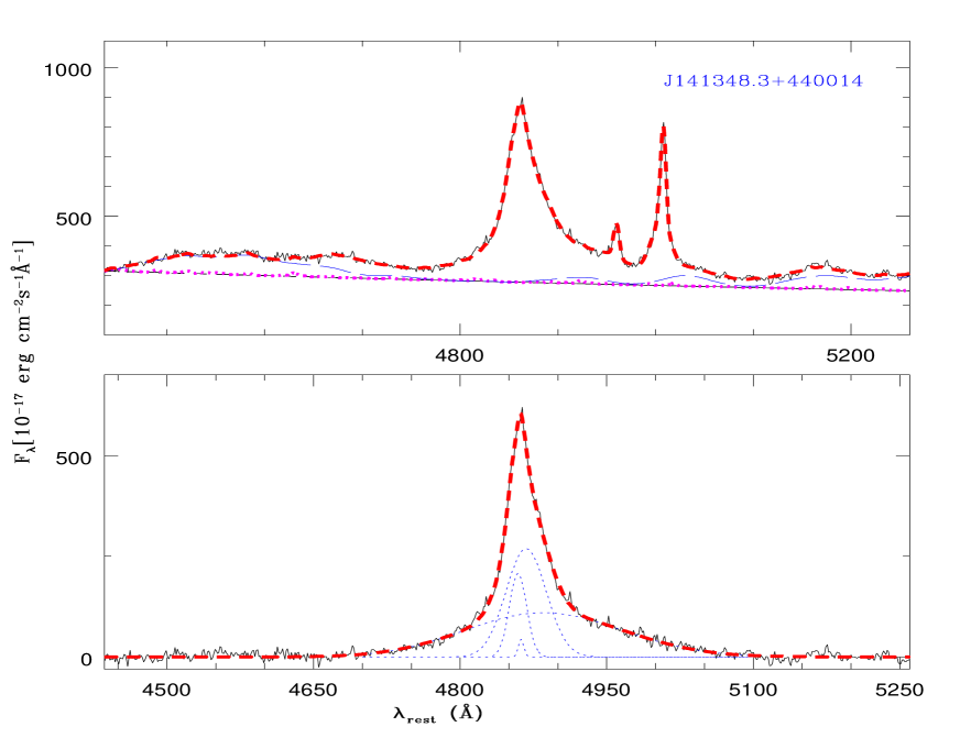
Figure 1: The best fit to the H$\beta$ emission line of the IGO spectra of the QSO J141348.3$+$440014. Upper panel: complete spectrum fit (thick dashed/red) and components of the fit: power law continuum (thin short-dashed/black line), broad Fe ii  (thin long-dashed/blue), narrow Fe ii  (dotted/magenta) lines. Lower panel: continuum, Fe ii  and metal line subtracted spectrum (solid/black) with the best fit total H$\beta$ profile (thick dashed/red) and H$\beta$  components (dotted/blue) lines. Note that the entire fit is performed simultaneously (not first continuum subtraction then H$\beta$ fit) but these aspects are shown separately for the sake of clarity.

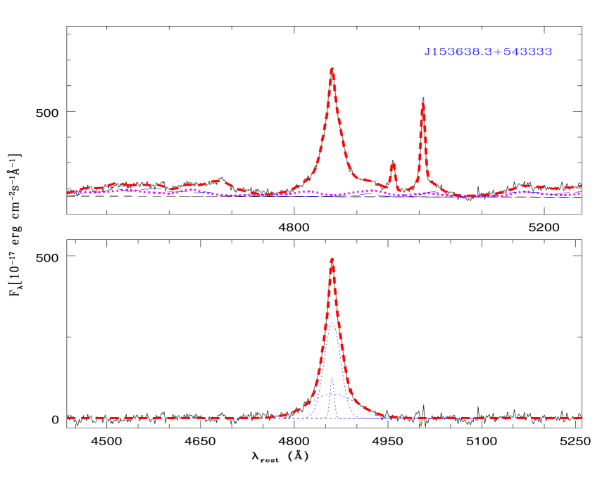
Figure 2: As in Fig. 1 IGO spectra for J153638.3$+$543333.

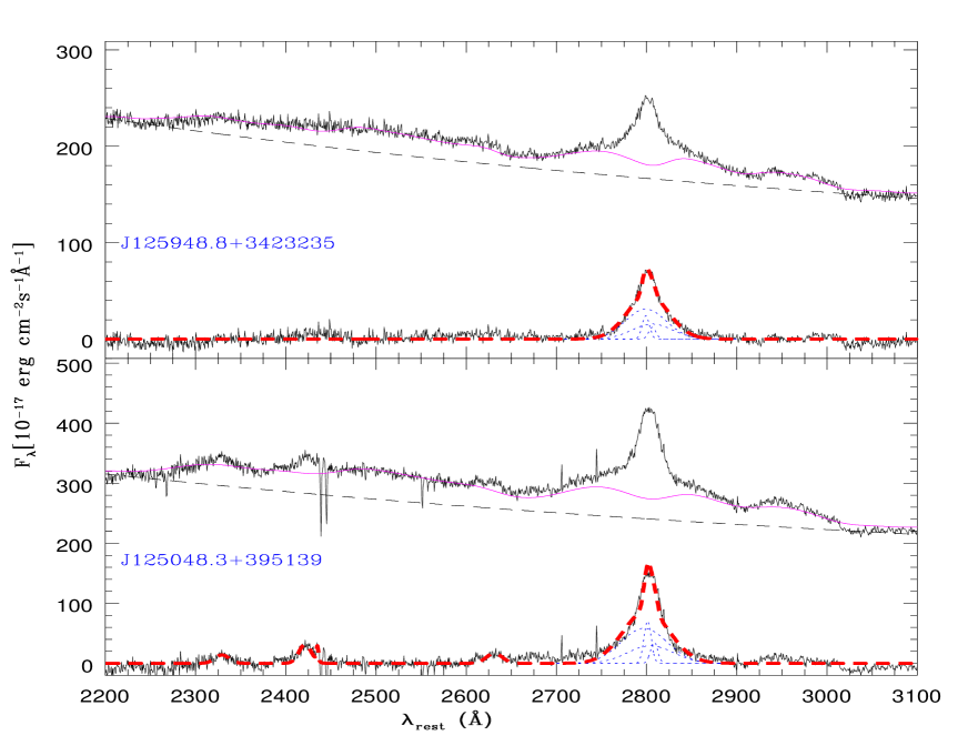
Figure 3: Mg ii emission line fits for two RQQSOs, J125948.8+342323.5 and J125048.3+395139. The upper plot in each panel shows the SDSS spectra and continuum as a dashed line with the best fit UV Fe ii  template as a solid (magenta) line. The lower plot in each panel show the continuum and Fe ii  subtracted spectrum (solid) the best fit Mg ii profile (thick dashed/red) and Mg ii$\lambda\lambda$2796,2803  components by (dotted/blue) lines. Note that the entire fits are performed simultaneously (not first continuum subtraction, then Mg ii fit) but are shown separately for the sake of clarity.

4.1 H$\beta$  region fit

(i) We fit the spectrum comprising the H$\beta$ line in the rest wavelength range between 4435 and 5535 Å. The continuum in this region is modeled by a single power law, i.e., $a_{1}\lambda^{-\alpha}$.

(ii) The complex profile of the H$\beta$ line is fitted with multiple (one to four) Gaussian with an initial guess of two narrow, one broad and one very broad components. To reduce the arbitrariness of the component fits and also to make the decomposition more physical, we have constrained the redshift and width of the two narrow components of H$\beta$ to be the same as those of the O iii$\lambda\lambda$4959,5007 lines. The line profile of O iii$\lambda$5007 (and hence of O iii$\lambda$4959 ) are modeled as double Gaussians, with one stronger narrow component with width less than 2000 km s${}^{-1}~{}$ and one weaker broader component with width less than 4000 km s${}^{-1}~{}$. However, if for some source spectra the second component is not statistically required, the procedure we use automatically drops it during the fit. So, we have only four free parameters, two for redshift and two for width, of the O iii$\lambda\lambda$4959,5007 and narrow H$\beta$  components.

(iii) The optical Fe ii  emission is modeled as $C(\lambda)=c_{b}C_{b}(\lambda)+c_{n}C_{n}(\lambda)$, where $C_{b}(\lambda)$ represents the broad Fe ii lines and $C_{n}(\lambda)$ the narrow Fe ii lines, with the relative intensities fixed at those of I ZW 1, as given in Tables A.1 and A.2 of Véron-Cetty, Joly & Véron (2004). The redshift of the broad Fe ii lines and the H$\beta$  component is fitted as a free parameter, while their widths are kept the same, with a constraint that they should be larger than 1000 km s${}^{-1}~{}$; this width is then used for estimating the BH masses. Similarly, for the narrow Fe ii line the redshift is fitted as a free parameter but the width is kept the same as that of the stronger narrow O iii$\lambda$5007 component. The fourth (very broad) H$\beta$ component, if required for the fit, is subject only to the constraint that its width should be more than 1000 km s${}^{-1}~{}$. The emission lines other than Fe ii and O iii$\lambda\lambda$4959,5007 (see Table 2 in Vanden Berk et al. 2001), are modeled with single Gaussians.

The final fit is achieved by simultaneously varying all the free parameters to minimize the $\chi^{2}~{}$ value until the reduced $\chi^{2}_{r}$ is $\approx 1$. Samples of our spectral fitting in the optical region are given for H$\beta$ in Fig. 1 and Fig. 2. The values for FWHM and EW (both the broad component, EW_B, and total, EW_all) for the H$\beta$ lines are given in Table 3.

4.2 Mg ii  doublet region fit

(i) We fit the spectrum comprising the Mg ii doublet region in the rest wavelength range between 2200 and 3200 Å. The continuum in this region is modeled by a single power law, i.e., $a_{1}\lambda^{-\alpha}$.

(ii) For fitting the Mg ii  doublet we have used a Gaussian profile model (Salviander et al. 2007) with the initial guess of two Gaussian components for each line of the Mg ii  doublet; however, if the second component is not statistically required the procedure automatically drops it during the fit. The redshift and width of each component (narrow/broad) of Mg ii$\lambda$2796  were tied to the respective components of the Mg ii$\lambda$2803 line. The peak intensity of Mg ii$\lambda$2796  was constrained to be twice that of Mg ii$\lambda$2803   as is predicted theoretically.

In addition, we have constrained the width of narrow component to be smaller than 1000 km s${}^{-1}~{}$  and the width of the broader Mg ii component to be same as width of UV Fe ii  emission line in the region (UV Fe ii ). We used an UV Fe ii template generated by Tsuzuki et al. (2006), basically from the measurements of I ZW 1, which also employ calculations with the CLOUDY photoionization code (Ferland et al. 1998). This template is scaled and convolved to the FWHM value equivalent to the broad components of Mg ii  by taking into account the FWHM of the I ZW 1 template. The best fit value of the broad component of Mg ii  obtained in this way is finally used in our calculation of BH mass. To test for any overfitting caused by assuming two components, we also forced our procedure to fit only single components; however, in doing so for all our sources, a very good fit is never found for the wings of the lines nor for their central narrow cores.

(iii) Emission lines other than Fe ii lines identified from the composite SDSS QSO spectrum (see Table 2 in Vanden Berk et al. 2001), are modeled with single Gaussians.

The final fit is achieved by varying all the free parameters simultaneously by minimizing the $\chi^{2}~{}$ value, until the reduced $\chi^{2}_{r}$ is $\approx 1$. Demonstrations of our spectral fitting in the UV region are given in Fig. 3, and values for FWMHs and EWs are given in Table 4.

4.3 Optical microvariability and spectral properties

The results from Paper I, with a modest sample of 37 sources, showed that the spectral properties for the sources with and without optical microvariability are quite similar. Here we search for better statistical results by adding our new 46 sources to the sample in Paper I. In these added 46 sources, among the 42 sources for which we have spectral coverage of the H$\beta$ line, 9 have shown optical microvariability while the other 33 have not been seen to show this property (Table 1). Of the 4 new sources with spectral coverage of the Mg ii doublet, not one showed optical microvariability. We now investigate the correlation between spectral properties (i.e., FWHM and EW) and optical microvariability with our best$-$fitting values and with the larger combined sample of 83 sources. Among the 53 sources with only H$\beta$ line coverage, optical microvariability is shown by 15 sources, while of the 22 sources with only Mg ii doublet spectral coverage, only 4 have been shown to exhibit microvariability properties. Of the remaining 8 source spectra that cover both Mg ii and H$\beta$ lines, optical microvariability was shown by one source.

From the multiple component fit of the H$\beta$ line we have used the broad component fit (Sect. 4.1) to perform the comparison. This is because the clouds responsible for this broad component are clearly in the sphere of influence of the massive BH, while the other components may not be. In Fig. 4 we show the histograms of FWHM and rest frame EW values based on our best fits for H$\beta$ and Mg ii lines. The shaded and non-shaded regions correspond respectively to sources with and without confirmed optical microvariability. From these plots it appears that the distributions of sources with and without microvariability are on the whole quite similar. To quantify any differences in these distributions we have performed Kolmogorov-Smirnov (KS) tests on all the distributions shown in Fig. 4. For the null hypothesis that the samples are drawn from the similar distributions we found the probabilities for the two $\rm H\beta(\rm EW)$ distributions to be 0.90 and for the two $\rm Mg~{}II(\rm EW)$ distributions to be 0.70. Similarly, we found the KS-tests null probability value for the two $\rm H\beta(\rm FWHM)$ distributions to be 0.29 and for the two $\rm Mg~{}II(\rm FWHM)$ distributions is 0.99.

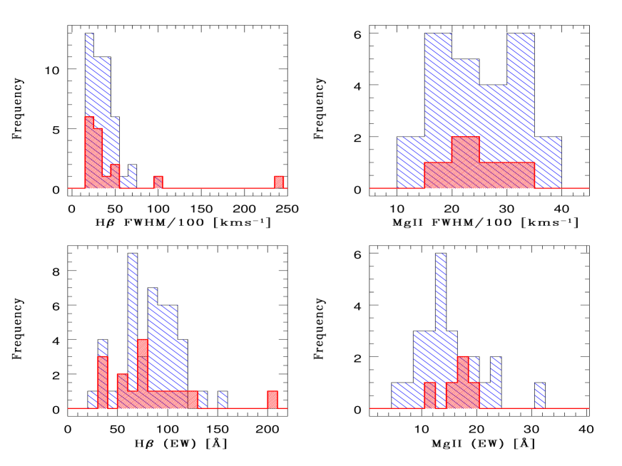
Figure 4: Histograms of FWHM and rest frame equivalent width (EW) based on best fits of H$\beta$ and Mg ii lines. The red (dark) shaded regions correspond to sources with confirmed optical microvariability while the striped regions correspond to those sources for which optical microvariability has not been detected.

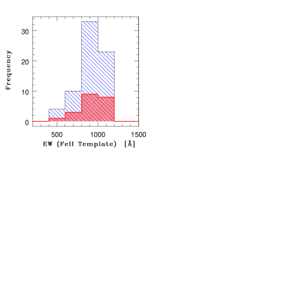
Figure 5: Histograms of EW of broad Fe ii template . The red (dark) shaded regions correspond to sources with confirmed optical microvariability while the striped regions correspond to those sources for which optical microvariability has not been detected.

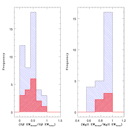
Figure 6: The left panel shows the histograms of the fraction of the broad H$\beta$ component in the H$\beta$ emission lines and the right panel shows the broad Mg ii component fraction in Mg ii emission lines.

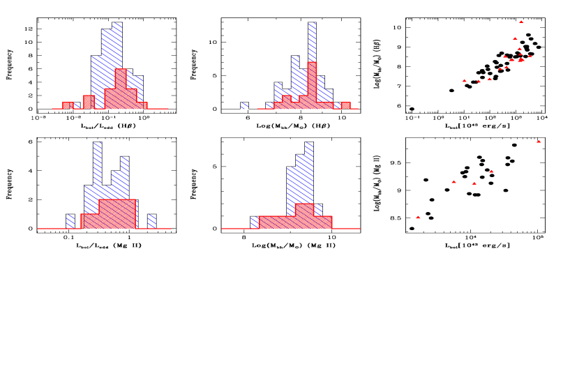
Figure 7: The upper left and middle panels show the histograms of Eddington ratio $L_{bol}/L_{edd}$ and ${\rm log}(M_{bh}/M_{\odot})$ based on the H$\beta$ line, while the corresponding bottom panels show the results based on the Mg ii line. The shaded regions correspond to sources with confirmed optical microvariability while the non-shaded regions are for those sources for which optical microvariability is not detected. The right upper and bottom panels respectively show plots of ${\rm log}(M_{bh}/M_{\odot})$ versus $L_{bol}$. Triangles and circles respectively show sources with and without confirmed optical microvariability.

In addition in the “blazar component” scenario one would also expect some dilution of emission line strength of the Fe ii template for microvariable sources. To test this possibility we have shown in Fig.  5 the EW distribution of broad Fe ii emission template for variable and non-variable sources, which by eye appear indistinguishable. The KS-test null probability value for these two Fe ii distributions is 0.72, and so does not give any hint of a blazar component. We have also tried to investigate the difference in fraction of broad components of H$\beta$ and Mg ii to the respective total line intensity for the sources with and without microvariability. We found that the distribution of this fraction of the H$\beta$ and Mg ii broad component is quite similar both for variable and nonvariable sources as is shown in Fig. 6.

The above substantial null-hypothesis probabilities do not establish any relation of EW or FWHM with the optical microvariability properties and thus do not support a blazar component model of microvariability for RQQSOs, which would predict smaller EW values for variable sources, due to dilution of emission line strength by jet components (Czerny et al. 2008). Here, the results drawn from a sample more than twice as large are in agreement with our results in Paper I.

Table 3: Results of the H$\beta$ line analysis

QSO Name	$z_{emi}$	$\frac{L(5100\AA)}{10^{43}\rm erg~{}s^{-1}}$	FWHM(km s-1)	log($\frac{M_{bh}}{M_{\odot}}$)	$\frac{L_{bol}}{L_{edd}}$	EWB(Å)	EWall(Å)
J000619.5$+$201210	0.0262	5.16	3292.99	7.80	0.06	54.10	$113.68\pm 0.33$
J002913.6$+$131603	0.1462	150.94	3615.62	8.62	0.25	17.30	$36.56\pm 0.31$
J004547.3$+$041024	0.3825	373.16	3025.37	8.66	0.55	31.97	$65.59\pm 0.53$
J005334.9$+$124136	0.0604	28.55	2095.22	7.78	0.32	31.49	$58.97\pm 0.32$
J005452.1$+$252538	0.1651	63.57	4272.75	8.57	0.11	54.00	$119.86\pm 0.62$
J011354.5$+$390744	0.2325	16.18	4179.08	8.26	0.06	46.60	$84.73\pm 1.18$
J012240.6$+$231015	0.0528	3.77	3136.91	7.69	0.05	0.93	$37.37\pm 0.49$
J051611.4$-$000859	0.0334	9.91	1654.62	7.35	0.30	3.48	$118.20\pm 0.22$
J051633.4$-$002713	0.2922	131.20	3959.10	8.66	0.19	61.56	$105.36\pm 0.48$
J055453.6$+$462622	0.0245	1.35	1882.71	7.03	0.09	24.15	$158.56\pm 0.59$
J071415.1$+$454156	0.0560	7.97	3822.48	8.03	0.05	42.88	$115.60\pm 0.51$
J073657.0$+$584613	0.0392	5.62	2868.64	7.70	0.08	39.24	$94.99\pm 0.41$
J084742.4$+$344504	0.0640	25.27	2406.85	7.87	0.23	4.87	$66.98\pm 0.27$
J092512.9$+$521711	0.0355	1.06	2657.45	7.27	0.04	53.63	$121.19\pm 0.63$
J092603.3$+$124404	0.0289	2.34	2024.97	7.21	0.10	18.53	$102.05\pm 0.47$
J095652.4$+$411522	0.2334	395.74	7136.27	9.42	0.10	47.62	$87.21\pm 0.36$
J101420.7$-$041840	0.0582	5.26	2180.48	7.45	0.13	16.03	$35.17\pm 0.61$
J105143.9$+$335927	0.1671	29.00	5980.04	8.69	0.04	7.75	$102.03\pm 0.76$
J110631.8$-$005252	0.4232	185.83	2465.65	8.33	0.59	54.71	$100.49\pm 0.68$
J111908.7$+$211918	0.1759	67.27	3197.73	8.33	0.21	83.05	$201.91\pm 0.72$
J112147.1$+$114418	0.0500	10.33	2322.45	7.65	0.16	33.37	$66.36\pm 0.35$
J112302.3$-$273004	0.3902	271.41	5058.81	9.03	0.17	64.23	$67.93\pm 0.47$
J112439.2$+$420145	0.2243	97.42	3519.45	8.50	0.21	2.34	$87.53\pm 0.54$
J115349.3$+$112830	0.1763	46.83	4711.23	8.59	0.08	58.22	$105.72\pm 0.59$
J120309.6$+$443153	0.0017	0.01	1617.19	5.84	0.01	18.63	$28.88\pm 1.20$
J121032.6$+$392421	0.0032	0.34	1997.36	6.78	0.04	22.95	$81.20\pm 0.17$
J132349.5$+$654148	0.1677	46.77	2857.81	8.16	0.22	40.22	$73.15\pm 0.65$
J140516.2$+$255534	0.1651	50.57	1912.69	7.83	0.51	45.00	$73.82\pm 0.49$
J141348.3$+$440014	0.0897	26.76	2923.47	8.06	0.16	48.78	$139.40\pm 0.70$
J141700.7$+$445606	0.1475	16.46	1534.52	7.39	0.45	2.79	$35.01\pm 0.63$
J142906.6$+$011706	0.0866	8.55	3100.99	7.86	0.08	19.46	$108.65\pm 0.85$
J144207.4$+$352623	0.0772	17.34	1723.99	7.50	0.37	40.97	$62.95\pm 0.51$
J153638.3$+$543333	0.0387	2.93	1918.30	7.21	0.12	54.76	$99.34\pm 0.69$
J155202.3$+$201402	0.2518	25.79	2108.52	7.76	0.30	56.78	$111.97\pm 1.06$
J162011.3$+$172428	0.1145	18.14	3814.02	8.20	0.08	13.63	$52.06\pm 0.99$
J170124.8$+$514920	0.2914	358.12	2656.36	8.54	0.71	23.23	$35.43\pm 1.70$
J175116.6$+$504539	0.2974	149.87	2484.15	8.29	0.52	40.79	$78.44\pm 0.41$
J211452.6$+$060742	0.4850	778.92	3695.78	8.99	0.54	73.60	$81.17\pm 0.53$
J213227.8$+$100819	0.0629	19.10	2870.28	7.97	0.14	57.01	$104.75\pm 1.60$
J221712.2$+$141421	0.0655	22.58	5499.40	8.57	0.04	77.21	$93.63\pm 1.55$
J230315.6$+$085226	0.0158	3.68	1888.66	7.24	0.14	22.62	$70.39\pm 0.84$
J230702.9$+$043257	0.0470	1.68	1667.88	6.97	0.12	8.19	$87.64\pm 1.31$

Table 4: Results of the Mg ii line analysis

QSO Name	$z_{emi}$	$\frac{L(3000\AA)}{10^{43}\rm erg~{}s^{-1}}$	FWHM(kms-1)	Log($\frac{M_{bh}}{M_{\odot}}$)	Log($\frac{M_{bh}}{M_{\odot}}$)	$\frac{L_{bol}}{L_{edd}}$	EWB(Å)	EWall(Å)
J112731.9$-$304446	0.6679	5691.58	1447.36	8.53	9.00	2.32	13.14	$13.14\pm 0.63$
J125048.3$+$395139	1.0318	1294.13	3029.19	8.78	9.32	0.25	19.64	$23.46\pm 0.31$
J125948.8$+$342323	1.3762	2577.21	3297.04	9.04	9.54	0.30	14.12	$16.28\pm 0.27$
J135458.7$+$005211	1.1253	1451.56	3007.11	8.80	9.34	0.27	22.30	$26.21\pm 0.17$

Table 5: BH growth time estimates (in units of Gyr) from the H$\beta$ line analysis

object	$z_{emi}$	Black hole growth time scale						age of the
		$L_{bol}$/$L_{edd}$ = 1.0			$L_{bol}$/$L_{edd}$ obs.			Universe
		$M_{bh}$(seed)			$M_{bh}$(seed)			(at $z_{emi}$)
		$10\,M_{\odot}$	$10^{3}\,M_{\odot}$	$10^{5}\,M_{\odot}$	$10\,M_{\odot}$	$10^{3}\,M_{\odot}$	$10^{5}\,M_{\odot}$	[$10^{9}$ yr]
J000619.5$+$201210	0.0262	0.68	0.48	0.28	12.40	8.75	5.11	13.11
J002913.6$+$131603	0.1462	0.76	0.56	0.36	3.09	2.28	1.47	11.62
J004547.3$+$041024	0.3825	0.77	0.57	0.37	1.38	1.02	0.66	9.33
J005334.9$+$124136	0.0604	0.68	0.48	0.28	2.12	1.50	0.87	12.66
J005452.1$+$252538	0.1651	0.76	0.56	0.36	6.60	4.86	3.11	11.41
J011354.5$+$390744	0.2325	0.73	0.53	0.33	11.94	8.65	5.36	10.70
J012240.6$+$231015	0.0528	0.67	0.47	0.27	12.90	9.05	5.19	12.76
J051611.4$-$000859	0.0334	0.64	0.44	0.24	2.11	1.44	0.78	13.01
J051633.4$-$002713	0.2922	0.77	0.57	0.37	4.00	2.96	1.91	10.12
J055453.6$+$462622	0.0245	0.60	0.40	0.20	7.03	4.70	2.37	13.13
J071415.1$+$454156	0.0560	0.71	0.50	0.30	13.82	9.89	5.96	12.71
J073657.0$+$584613	0.0392	0.67	0.47	0.27	8.84	6.20	3.56	12.93
J084742.4$+$344504	0.0640	0.69	0.49	0.29	3.02	2.14	1.26	12.61
J092512.9$+$521711	0.0355	0.63	0.43	0.23	16.55	11.27	5.99	12.98
J092603.3$+$124404	0.0289	0.62	0.42	0.22	6.36	4.31	2.26	13.07
J095652.4$+$411522	0.2334	0.84	0.64	0.44	8.20	6.25	4.30	10.69
J101420.7$-$041840	0.0582	0.65	0.45	0.25	5.09	3.51	1.93	12.69
J105143.9$+$335927	0.1671	0.77	0.57	0.37	19.28	14.27	9.25	11.39
J110631.8$-$005252	0.4232	0.74	0.53	0.33	1.25	0.91	0.57	9.00
J111908.7$+$211918	0.1759	0.74	0.53	0.33	3.48	2.53	1.58	11.29
J112147.1$+$114418	0.0500	0.67	0.47	0.27	4.25	2.97	1.69	12.79
J112302.3$-$273004	0.3902	0.81	0.60	0.40	4.77	3.58	2.39	9.26
J112439.2$+$420145	0.2243	0.75	0.55	0.35	3.58	2.63	1.67	10.78
J115349.3$+$112830	0.1763	0.76	0.56	0.36	9.40	6.92	4.44	11.29
J120309.6$+$443153	0.0017	0.49	0.28	0.08	48.54	28.48	8.42	13.44
J121032.6$+$392421	0.0032	0.58	0.38	0.18	14.86	9.72	4.58	13.42
J132349.5$+$654148	0.1677	0.72	0.52	0.32	3.26	2.35	1.44	11.38
J140516.2$+$255534	0.1651	0.68	0.48	0.28	1.34	0.95	0.56	11.41
J141348.3$+$440014	0.0897	0.71	0.51	0.31	4.45	3.19	1.93	12.29
J141700.7$+$445606	0.1475	0.64	0.44	0.24	1.41	0.97	0.53	11.61
J142906.6$+$011706	0.0866	0.69	0.49	0.29	8.60	6.09	3.59	12.33
J144207.4$+$352623	0.0772	0.65	0.45	0.25	1.77	1.23	0.68	12.45
J153638.3$+$543333	0.0387	0.62	0.42	0.22	5.10	3.46	1.82	12.94
J155202.3$+$201402	0.2518	0.68	0.48	0.28	2.26	1.59	0.92	10.51
J162011.3$+$172428	0.1145	0.72	0.52	0.32	9.38	6.77	4.17	11.99
J170124.8$+$514920	0.2914	0.76	0.56	0.36	1.07	0.79	0.50	10.13
J175116.6$+$504539	0.2974	0.73	0.53	0.33	1.40	1.02	0.63	10.07
J211452.6$+$060742	0.4850	0.80	0.60	0.40	1.49	1.12	0.75	8.53
J213227.8$+$100819	0.0629	0.70	0.50	0.30	5.03	3.59	2.14	12.63
J221712.2$+$141421	0.0655	0.76	0.56	0.36	18.52	13.62	8.73	12.59
J230315.6$+$085226	0.0158	0.63	0.43	0.22	4.44	3.02	1.59	13.25
J230702.9$+$043257	0.0470	0.60	0.40	0.20	4.87	3.24	1.61	12.83

Table 6: BH growth time estimates (in units of Gyr) from the Mg ii line analysis

object	$z_{emi}$	Black hole growth time scale						age of the
		$L_{bol}$/$L_{edd}$ = 1.0			$L_{bol}$/$L_{edd}$ obs.			Universe
		$M_{bh}$(seed)			$M_{bh}$(seed)			(at $z_{emi}$)
		$10\,M_{\odot}$	$10^{3}\,M_{\odot}$	$10^{5}\,M_{\odot}$	$10\,M_{\odot}$	$10^{3}\,M_{\odot}$	$10^{5}\,M_{\odot}$	[$10^{9}$ yr]
J112731.9$-$304446	0.6679	0.80	0.60	0.40	0.35	0.26	0.17	7.35
J125048.3$+$395139	1.0318	0.83	0.63	0.43	3.34	2.54	1.73	5.63
J125948.8$+$342323	1.3762	0.86	0.66	0.46	2.85	2.19	1.52	4.52
J135458.7$+$005211	1.1253	0.84	0.64	0.44	3.10	2.35	1.61	5.29

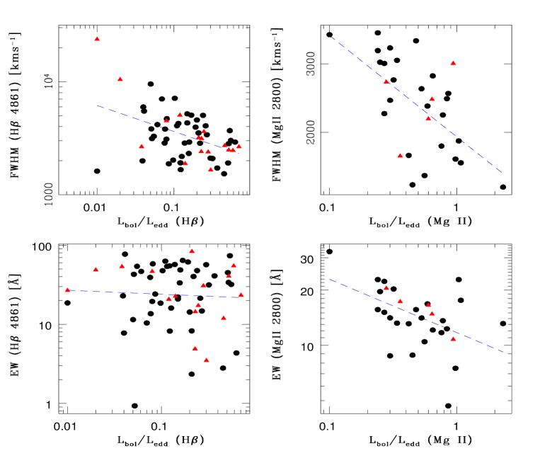
Figure 8: Observed variation of FWHM (upper) and EW (lower) with Eddington ratio ($\ell={\rm L}_{bol}/{\rm L}_{edd}$) based on both H$\beta$ (left) and Mg ii (right) lines. Triangles and circles respectively show sources with and without confirmed optical microvariability. The dashed lines show the linear regression fits treating $\ell$ as the independent variable. The correlations of both FWHM and EW with $\ell$, suggest that the Eddington ratio is one of the fundamental parameters responsible for some AGN properties.

5 Black Hole Mass Measurements, Eddington ratios and black hole growth times

We have estimated the black hole masses using the virial single epoch method (Dibai 1980), following the approach in Paper I. This method has been shown to be consistent with reverberation mapping masses (e.g., Bochkarev & Gaskell 2009). Improved empirical relationships (e.g., Vestergaard & Peterson 2006) are used for estimating the central BH mass based on FWHMs of emission lines such as H$\beta$ and Mg ii. We used Eq. 1 and Eq. 2 in Paper I, taken from Vestergaard & Peterson (2006) and McLure & Dunlop (2004), to determine respectively black hole masses based on H$\beta$ lines and Mg ii lines, viz;

$$\log\,M_{\rm BH}(\rm H\beta)=\log\,\left[\left(\frac{\rm FWHM(H\beta)}{1000~{}km~{}s^{-1}}\right)^{2}\right]$$ (1)

$$\mbox{}+(6.91\pm 0.02)+\log\,\left(\frac{\lambda\it L_{\lambda}{\rm(5100\,\AA)}}{10^{44}\rm erg~{}s^{-1}}\right)^{0.50\pm 0.06},$$

$$\log\,M_{\rm BH}(\rm Mg~{}II)=(0.62\pm 0.14)\log\left(\frac{\lambda\it L_{\lambda}\rm(3000\,\AA)}{10^{44}\rm erg~{}s^{-1}}\right)$$ (2)

$$\mbox{}+2\log\left(\frac{\rm FWHM(Mg~{}II)}{\rm kms^{-1}}\right)+0.505$$

where $L_{\lambda}{\rm(5100\,\AA)}$ & $L_{\lambda}{\rm(3000\,\AA)}$ are the monochromatic luminosity at 5100 Å  and 3000 Å , respectively, which we have computed from the best fit power-law continuum, $a_{1}\lambda^{-\alpha}$, in our simultaneous fit of the whole spectral region.

We have also estimated the Eddington ratio $\ell\equiv L_{bol}/L_{edd}$, where $L_{bol}$ is taken as $5.9\times\lambda L_{\lambda}$(3000Å) and $9.8\times\lambda L_{\lambda}$(5100Å) for Mg ii and H$\beta$ , respectively (McLure & Dunlop 2004), and $L_{edd}=1.45\times 10^{38}(M_{bh}/M_{\odot})\ \ \rm erg~{}s^{-1}$, assuming a mixture of hydrogen and helium so the mean molecular weight is $\mu=1.15$. The combined sample results are given in Fig. 7, which by eye indicates that distributions of sources with and without optical microvariability appear similar with respect to both BH mass and $\ell$. Quantitatively, this is also supported by KS tests, which show that the probability of the null hypothesis ($P_{null}$) for sources with and without microvariation, is as high as 0.69 for BH mass distributions and 0.11 for Eddington ratio ($\ell$) distributions based on H$\beta$ lines fit. Similarly using Mg ii lines, the null hypothesis ($P_{null}$) for sources with and without microvariation, is as high as 0.98 for BH mass distributions and 0.94 for Eddington ratio ($\ell$) distributions.

To test the reasonableness of estimated Eddington ratios, we also computed black hole growth times to compare them with the age of the Universe (at the time the QSO is observed), by using the following equation (Dietrich et al. 2009),

$$M_{bh}(t_{obs})=M_{bh}^{seed}(t_{0})\,{\rm exp}\biggl{(}\ell\,{(1-\epsilon)\over\epsilon}\,{\tau\over t_{edd}}\biggr{)}~{},$$ (3)

where $\tau=t_{obs}-t_{0}$ is the time elapsed since the initial time, $t_{0}$, to the observed time, $t_{obs}$; $M_{bh}^{seed}$ is the seed BH mass; $\epsilon$ is the efficiency of converting mass to energy in the accretion flow, and $t_{edd}$ is the Eddington time scale, with $t_{edd}=\sigma_{T}c/4\pi Gm_{p}=3.92\times 10^{8}$ yr (Rees 1984). We used Eq. 3 to derive the times, $\tau$, necessary to accumulate the BH masses listed in Tables 3 and 4, for seed black holes with masses of $M_{bh}^{seed}=10M_{\odot}$, $10^{3}M_{\odot}$, and $10^{5}M_{\odot}$, respectively. Two cases are considered: (i) BHs are accreting at the Eddington-limit, i.e., $\ell$ = L_bol/L_edd = 1.0 and the efficiency of converting mass into energy is $\epsilon=0.1$; (ii) BHs are accreting with our observed Eddington ratios and $\epsilon=0.1$. These results are summarized in Tables 5 and 6, showing that the key criterion that black hole growth time should be smaller than the age of Universe is fulfilled for all sources.

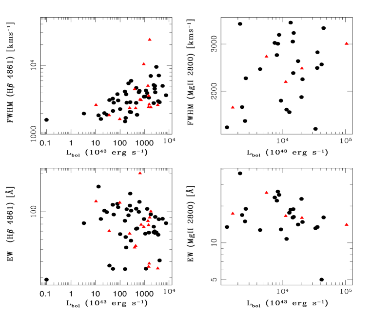
Figure 9: As in Fig. 8 with $L_{\rm bol}$ as the independent variable. This panel indicates that the sources with and without optical microvariability are similar in luminosity.

In our Paper I we found a weak negative correlation between H$\beta$ EW and the Eddington ratio, $\ell$, and a significant one between the Mg ii EW and $\ell$. In Fig. 8 we show the observed variations of FWHM and EW with $\ell$ based on both H$\beta$ and Mg ii lines for our combined sample. There appear to be linear relations of both FWHM and EW with $\ell$ in these log-log plots. For the FWHM plots this is unsurprising since the BH masses are proportional to $L_{edd}$. To quantify any such linear relations for the EW plots we perform linear regressions, treating $\ell$ as the independent variable, and find

$$\rm logEW(H\beta)=(1.33\pm 0.12)+(-0.05\pm 0.13)\rm log(\ell),$$

$$\rm logEW(\rm Mg~{}II)=(1.07\pm 0.04)+(-0.29\pm 0.10)\rm log(\ell).$$ (4)

Here the errors on the fit parameters are purely statistical. We have calculated the Spearman rank correlations of logEW with log$\ell$, and found the correlation coefficient for r${}_{s}(H\beta)=-0.05$, with null probability $p_{null}=0.72$, and so no significant correlation is present. Whereas r${}_{s}(\rm Mg~{}II)=-0.45$, with $p_{null}=0.013$ and so this negative correlation is significant. These results are in agreement with those from our Paper I that were based on a modest sample size.

6 Discussion and Conclusions

Modern surveys such as SDSS have allowed investigators to carry out spectral analyses of large numbers of quasars to estimate central BH masses using virial approaches (e.g., Shen et al. 2008; Fine et al. 2008; Vestergaard & Osmer 2009) and to understand their demography (Dong et al. 2009b). These studies have resulted in very important insights on the important physical parameters of AGN central engines and their environments.

Dong et al. (2009b) found that the variation of the emission-line strength in AGNs are regulated by $\ell$, presumably because it governs the global distributions of the properties such as column density of the clouds gravitationally bound in line emitting region. Shen et al. (2008) have found that the line widths of H$\beta$ and Mg ii follow lognormal distributions with very weak dependencies on redshift and luminosity. Fine et al. (2008) used Mg ii lines to estimate BH masses, and found that the scatter in measured BH masses is luminosity dependent, showing less scatter for more luminous objects.

The sample we have considered more than doubles our sample in Paper I, but still is much smaller compared to those in the above papers, that consist of between 1100 and almost 57,700 quasars. However, each member in our sample has been carefully selected to be among the special group of RQQSOs and Seyfert galaxies already examined for optical microvariability (e.g., Carini et al. 2007). This criterion demands that modest aperture (usually 1–2 m) telescopes can make precise photometric measurements in just a few minutes, and so limits the members to the rare QSOs with bright apparent magnitudes (usually $m_{V}<17.5$). In addition, we have taken special care in the fitting of the line profiles as discussed in Sections 4.1 and 4.2.

It has been found that for BL Lacertae objects the emission line detection and strength varies with overall continuum flux (e.g., Nilsson et al. 2008). For instance, when BL Lacs are in optically faint states weak emission lines have sometimes been detected that are usually not seen during their high states, presumably due to their being swamped by the Doppler boosted continuum arising in a strong jet component (Nilsson et al. 2009).

To check whether the continuum states of our objects, high (bright) or low (faint), have any such effect on their spectral properties, we have searched in the SDSS DR8 archive for multi-epoch photometric and spectroscopic observations for the 44 SDSS sources in our sample. We found multi-epoch photometric fluxes were available for 14 sources, with time gaps ranging from a few days to years. We then searched for spectroscopic observations of these sources and found multi-epoch spectra are available only for three sources, viz. J025937.46$+$003736.3; J084030.0$+$465113; J093502.6$+$433111. Among them, J093502.6$+$433111 has two spectra with a roughly one year time gap (observations on 2002 Feb 20 and 2003 Jan 31) but only a single photometric data point at all close to either of those dates (2001 Dec 20). For J084030.0$+$465113 two spectra were available about a month apart (2001 Jan 13 and 2001 Feb 19) but these had their two closest photometric observations made on 2001 Jan 24 and 2001 Jan 26, respectively. As these two photometric observations have only a two day time gap and have a g-mag difference of only 0.01 this object also does not serve to test for such a correlation. We are left with just one source, J025937.46$+$003736.3, that has both photometric and spectroscopic multi-epoch data that are well paired. For this source there were two spectral observations on 2000 Nov 25 and 2001 Sep 21 and corresponding photometric observations on 2000 Nov 27 and 2001 Sep 21 with g$-$mags of 16.41 and 16.47, respectively. As this g$-$mag difference of 0.06 is much larger than the typical RQQSOs INOV magnitude variation of about 0.01 mag over a night, this source is the only one that might test whether brighter or fainter states have any significant effect on spectral properties. Even though this difference in brightness is modest, we carried out our spectral fits to each of those two spectra to estimate the FWHMs and EWs of the H$\beta$ line, using the same method as we used for other sources (Sect. 4.1). The best fit EW(H$\beta$ ) of broad component for first epoch was found to be $30.47\pm 0.63$Å and for second epoch, $29.23\pm 0.45$Å. These values are statistically indistinguishable, so there is no evidence for any effect due to variation in source brightness. However, in order to say anything firm about this possibility for RQQSOs, nearly simultaneous spectroscopic and photometric measurements would need to be made on at least two occasions for a decent sized sample.

In this paper we continued our work begun in Paper I with 37 RQQSOs by analyzing spectra for an additional 46 sources. Most of these spectra were obtained by us at the IGO. We conclude that there is a significant negative correlation between Mg ii EW and $\ell$, (Fig. 8; Section 5), as also found in Paper I (there Fig. 7) and by Dong et al. (2009b). However, we have not found any significant correlation between the equivalent widths of the H$\beta$ lines and the Eddington ratio, $\ell$. We can also see from Fig. 8 that there is a decline in FWHM with $\ell$; this is not surprising since the BH masses are proportional to $L_{edd}$. In Paper I (Fig. 8), we noticed a interesting tendency for sources with detectable optical microvariability to have somewhat lower luminosity than those with no such detections, which required investigation with a larger sample. One might expect such a trend, as lower mass BHs would have correspondingly shorter physical timescales. However, as can be seen from Fig. 9 there is no such trend seen with our new larger sample of microvariable sources (16 as compared to 7 in Paper I).

We also find that the BH masses estimated from the FWHMs of both the H$\beta$ and Mg ii lines are reasonable, in that growth to their estimated masses from even small seed BHs are easily possible within the age of the Universe at their observed redshift if the mean $\ell$ values are close to unity (Tables 5 and 6). This remains true for the great majority of RQQSOs even if the value of $\ell$ we compute from the current continuum flux was constant until the time we observe them; however, this assumption does not work for 8 out of the 42 QSOs with H$\beta$ lines, while we consider $M_{bh}(seed)=10M_{\odot}$, for 4 while we consider $M_{bh}(seed)=10^{3}M_{\odot}$ and for none while we consider $M_{bh}(seed)=10^{5}M_{\odot}$, suggesting that in a few cases $M_{bh}(seed)$ could need to be as large as $10^{5}M_{\odot}$ or the accretion rate was substantially higher in the past. With Mg ii lines profiles no QSO was found problematic with respect to this assumption (Table 6).

As Fig. 4 shows, histograms of FWHM and rest frame EW values for sources with and without confirmed optical microvariability are on the whole quite similar. Under the null hypothesis that the samples are drawn from the similar distribution using KS-tests we find a probability of 0.90 for the $\rm H\beta(\rm EW)$ distributions and 0.70 for the $\rm Mg~{}II(\rm EW)$ distributions. Similarly this null probability for the FWHM distributions is 0.29 for $\rm H\beta(\rm FWHM)$ and 0.99 for $\rm Mg~{}II(\rm FWHM)$ distributions. We conclude that EW or FWHM distributions (for both the H$\beta$ or Mg ii ) are probably independent of the presence or absence of detected microvariability properties in those QSOs and Seyferts. As discussed in the Introduction and in more detail in Paper I, if much of the optical emission in RLQSOs comes from a jet, then we would expect the EWs of the RLQSOs to be significantly lower than those of the RQQSOs and that the EWs of microvariable sources would be less than those of non-variable sources. Our results are in agreement to the conclusion in Paper I and thus do not support the hypothesis (e.g., Gopal-Krishna et al. 2003; Czerny et al. 2008) that RQQSOs possess jets that are producing rapid variations. Instead it may indicate that variations involving the accretion disc (e.g., Wiita 2006) play an important role here.

Further improvements to our results could be obtained through extensive searches for INOV in a larger sample of RQQSOs to reduce the statistical uncertainties. In any such studies it would be most useful to take the spectra just before or after the photometric monitoring run, so as to ensure the simultaneity of light curve and spectral properties. This would rule out any possibility of change in either of these properties due to temporal gaps between the spectral and photometric epochs; while we very much doubt that this is an important effect, it could have an impact on our results. Such larger samples could be optimally designed if they were made as homogeneous as possible on the basis of apparent magnitudes, redshifts and absolute magnitudes.

References

- Abazajian et al. (2009) Abazajian K. N., Adelman-McCarthy J. K. Agüeros, M. A., et ANAal., 2009, ApJS, 182, 543
- Aihara et al. (2011) Aihara H., et al., 2011, ApJS, 193, 29
- Bochkarev & Gaskell (2009) Bochkarev N. G., Gaskell, C. M., 2009, Astron. Lett., 35, 287
- Boroson & Green (1992) Boroson T. A., Green R. F., 1992, ApJS, 80, 109
- Carini et al. (2007) Carini M. T., Noble J. C., Taylor R., Culler R., 2007, AJ, 133, 303
- Chand et al. (2010) Chand H., Wiita P. J., Gupta A. C., 2010, MNRAS, 402, 1059 (Paper I)
- Czerny et al., (2008) Czerny B., Siemiginowska A., Janiuk A., Gupta A. C., 2008, MNRAS, 386, 1557
- Dibai (1992) Dibai É. A., 1980, Sov. Astron., 24, 389
- Dietrich et al. (2009) Dietrich M., Mathur S., Grupe D., Komossa S., 2009, ApJ, 696, 1998
- Dong et al. (2009a) Dong X.-B, Wang J.-G, Wang T.-G, Wang H., Fan X., Zhou H., Yuan, W., 2009a, arXiv:0903.5020
- Dong et al. (2009b) Dong X.-B., Wang T.-G., Wang J.-G., Fan X., Wang H., Zhou H., Yuan W., 2009b, ApJL, 703, L1
- Ferland et al. (1998) Ferland G. J., Korista K. T., Verner D. A., Ferguson J. W., Kingdon J. B., Verner, E. M., 1998, PASP, 110, 761
- Fine et al. (2008) Fine S., Croom S. M., Hopkins P. F., et al., 2008, MNRAS, 390, 1413
- Fitzpatrick (1999) Fitzpatrick E. L., 1999, PASP, 111, 63
- Gaskell C. M., (2006) Gaskell C. M., 2006, in Gaskell C. M., McHardy I. M., Peterson B. M., Sergeev S. G., eds, ASP Conf. Ser. Vol. 360, AGN Variability from Xrays to Radio Waves. Astron. Soc. Pac., San Francisco, p. 111
- Gopal-Krishna et al. (2003) Gopal-Krishna, Stalin C. S., Sagar R., Wiita P. J., 2003, ApJ, 586, L25
- Gupta al. al (2005) Gupta A. C., Joshi U. C. 2005, A&A, 440, 855
- Joshi et al. (2011) Joshi R., Chand H., Gupta A. C., Wiita P. J. 2011, MNRAS, 412, 2717
- Kim et al. (1995) Kim D.-C., Sanders D. B., Veilleux S., Mazzarella J. M., Soifer B. T., 1995, ApJS, 98, 129
- Mangalam & Wiita (1993) Mangalam A. V., Wiita P. J., 1993, ApJ, 406, 420
- McLure & Dunlop (2004) McLure R. J., Dunlop J. S., 2004, MNRAS, 352, 1390
- Moustakas & Kennicutt (2006) Moustakas J., Kennicutt R. C., Jr., 2006, ApJS, 164, 81
- Nilsson et al. (2008) Nilsson K., Pursimo T., Sillanpää A., Takalo L. O., Lindfors E., 2008, A&A, 487, L29
- Nilsson et al. (2009) Nilsson K., Pursimo T., Villforth C., Lindfors E., Takalo L. O., 2009, A&A, 505, 601
- Rees (1984) Rees M. J., 1984, ARA&A, 22, 471
- Rokaki et al. (1993) Rokaki E., Collin-Souffrin S., Magnan C., 1993, A&A, 272, 8
- Salviander et al. (2007) Salviander S., Shields G. A., Gebhardt K., Bonning E. W.,2007, ApJ, 662, 131
- Schlegel, Finkbeiner, & Davis (1998) Schlegel D. J., Finkbeiner D. P., Davis M., 1998, ApJ, 500, 525
- Shen et al. (2008) Shen Y., Greene J. E., Strauss M. A., Richards G. T., Schneider D. P., 2008, ApJ, 680, 169
- Tsuzuki et al. (2006) Tsuzuki Y., Kawara K., Yoshii Y., Oyabu S., Tanabé T., Matsuoka Y. 2006, ApJ, 650, 57
- Vanden Berk et al. (2001) Vanden Berk D. E., Richards G. T., Bauer, A., et al., 2001, AJ, 122, 549
- Véron-Cetty et al. (2004) Véron-Cetty M.-P., Joly M., Véron P., 2004, A&A, 417, 515
- Vestergaard & Osmer (2009) Vestergaard M., Osmer P. S., 2009, ApJ, 699, 800
- Vestergaard & Peterson (2006) Vestergaard M., Peterson B. M., 2006, ApJ, 641, 689
- Wiita (2006) Wiita P. J. 2006, in H. R. Miller, K. Marshall, J. R. Webb & M. F. Aller, eds, ASP Conf. Ser. Vol. 300, Blazar Variability II: Entering the GLAST Era. Astron. Soc. Pac., San Francisco, p. 183