Gap size and capture zone distributions in one-dimensional point island nucleation and growth simulations: asymptotics and models

Abstract

The nucleation and growth of point islands during submonolayer deposition on a one-dimensional substrate is simulated for critical island size $i=0,1,2,3$. The small and large size asymptotics for the gap size and capture zone distributions (GSD and CZD) are studied. Comparisons to theoretical predictions from fragmentation equation analyses are made, along with those from the recently proposed Generalised Wigner Surmise (GWS). We find that the simulation data can be fully understood in the framework provided by the fragmentation equations, whilst highlighting the theoretical areas that require further development. The GWS works well for the small-size CZD behaviour, but completely fails to describe the large-size CZD asymptotics of the one-dimensional system.

I INTRODUCTION

The nucleation and growth of islands during submonolayer deposition is of considerable theoretical interest as a fundamental problem in the statistical mechanics of growth processes Barabasi95 ; Venables84 ; Amar01 ; PAM08 ; PAM09 . The sizes and spatial organisation of the nucleated islands ultimately determine the higher-level structures such as film and nanostructure array morphologies Evans06 . A long-established strategy in the analysis of the statistical properties is to study capture zones of islands, since these not only reflect spatial organisation but also determine growth rates of the islands PAM95 ; PAM96 ; Bartelt98 ; PAM00 ; Evans02 ; PAM04 . Therefore, the evolution of capture zones during the deposition process has been a focus of many recent theoretical works PE07 ; Li10 ; PE10 ; Shi09 ; Oliv11 .

Recently, Pimpinelli and Einstein introduced a new theory for the capture zone distribution (CZD) employing the Generalised Wigner Surmise (GWS) from random matrix theory PE07 , causing some controversy. Oliveira and Reis Oliv11 have presented simulation results for islands grown on a two-dimensional substrate with critical island size $i=1$ and $2$, providing some support for the proposed Gaussian tail of the CZD PE07 . However, Li et. al. Li10 presented an alternative theory which yields a modified form for the large-size CZD behaviour, supported by data for the simulated growth of compact islands with $i=1$. This form seems to agree with that found by Oliveira and Reis, contradicting the GWS Oliv11 . In other work, Shi et. al. Shi09 studied $i=1$ models in $d=1,2,3,4$ dimensions, finding that the CZD is more sharply peaked and narrower than the GWS suggests. Therefore it is by no means established whether the GWS provides a good theoretical basis for understanding the distribution of capture zones found in island nucleation and growth simulations.

The simplified case of point island nucleation and growth in one dimension has proven to be a good test case for theories. For example, Tokar and Dreyssé T&D08 have recently used this model to illustrate their accelerated kinetic Monte Carlo algorithm for diffusion limited kinetics, finding excellent scale invariance in the island size distribution. Blackman and Mulheran BM96 studied the system with critical island size $i=1$, using a fragmentation equation approach. In this system, we can view the substrate as a string of inter-island gaps, and new island nucleation caused by the deposited monomers as a fragmentation of these gaps. Thus in order to understand the CZD, it is important first to be able to describe the gap size distribution (GSD).

In recent work GLOM11 we have extended the analysis of the fragmentation equations of [BM96, ] to the case of general $i=0,1,\ldots$. We have been able to derive the small and large size asymptotics of the GSD, and by assuming random mixing of the gaps caused by the nucleation process, we have also derived the small size asymptotics for the CZD for general $i$ and the large size behaviour for $i=0$.

One key feature to emerge from this work is that the asymptotic behaviour of the CZD is again different to that of the GWS PE07 . It therefore is appropriate to ask what support, further to that in reference [BM96, ], for the fragmentation equation approach is offered by Monte Carlo simulations of the system. Recent work by Gonzalez et. al. GPE11 has revisited the case of $i=1$, developing the original fragmentation equation BM96 and GWS arguments in response to deviations between prediction and simulation. In this work we will explore simulation results for the one-dimensional (1-D) model with $i=0,1,2,3$, and consider the relative merits of the fragmentation theory GLOM11 and GWS PE07 approaches.

The paper is organised as follows. In Section II we summarise the relevant theoretical results GLOM11 ; PE07 . In Section III we describe the Monte Carlo methods used in our work, both for the full simulation of the island nucleation and growth processes as well as for nucleation within single gaps. Simulation results are presented in Section IV and compared to theoretical predictions, and we finish with a summary and our conclusions in Section V.

II THEORY AND PREDICTIONS

The data from MC simulations can be used as a benchmark against which to test predictions of theories for the GSD and CZD. In the next two subsections, we will discuss the predictions of two competing theories, namely the fragmentation equation approach and the GWS.

II.1 Fragmentation Equations

We follow the Blackman and Mulheran approach for the 1-D point-island model with $i=1$ BM96 . Island nucleation events are viewed as the fragmentation of gaps between stable islands; see Figure 1. A nucleation that occurs in a parent gap of width $y$ will result in the creation of two daughter gaps of widths $x$ and $y-x$. The probability that the nucleation occurs at position $x<y$ is taken from the long-time (steady state) monomer density profile in the gap,

$$n_{1}(x)=\frac{1}{2R}x(y-x),$$ (1)

where $R=D/F$ is the ratio between the monomer diffusion constant $D$ and the monomer deposition rate $F$. In particular, we assume that the nucleation probability is obtained from this monomer density $n_{1}(x)^{\alpha}$, with the value of $\alpha$ reflecting the nucleation process. We then obtain GLOM11

$$\frac{\partial}{\partial t}u(x,t) = -B(\alpha+1,\alpha+1)x^{\lambda}u(x,t)$$ (2)

$$+ 2\int_{x}^{\infty}[x(y-x)]^{\alpha}u(y,t)dy,$$

where $B(\cdot,\cdot)$ is the Beta function and $\lambda=2\alpha+1$. Here, $u(x,t)$ is the number of gaps of size $x$ at time $t$. The first term on the right hand side of (2) is the rate at which gaps of size $x$ are removed from the population by a nucleation event. The second term describes the creation of gaps of size $x$ from the fragmentation of larger gaps, with the factor $2$ reflecting the symmetry of the fragmentation kernel.

Figure 1: Summary of the features of the one-dimensional point island model with $i=1$. Solid circles represent an island; open circles are monomers. A capture zone is the separation of the bisectors of neighbouring gaps.BM96

In [GLOM11, ] we set $\alpha=i+1$ under the assumption that nucleation is a rare event solely driven by the diffusion of the monomers. In doing this we implicitly assume that the $i+1$ monomers necessary to create the nucleus are all in some sense mature, each separately obeying the long-time steady-state density profile $n_{1}(x)$. However, we shall also have need to consider the case when nucleation is triggered by a deposition event. Here a newly deposited monomer either lands close to (or even directly onto) a pre-existing cluster of $i>0$ mature monomers. In this case, we set $\alpha=i$.

Eqn. (2) admits similarity solutions of the form ZM86 ; CR88 ; EMR05 ; GLOM11

$$u(x,t)=\bar{x}(t)^{-2}\phi(x/\bar{x}(t)),$$ (3)

where $\bar{x}(t)$ is the average gap size. The following asymptotics are then found GLOM11 :

$$\phi(z)\sim kz^{\alpha}\mbox{ as }z\rightarrow 0;$$ (4)

$$\phi(z)\sim kz^{-2}\exp(-cz^{\lambda})\mbox{ as }z\rightarrow\infty,$$ (5)

for constants $c>0$ and $k$. Here $z=x/\bar{x}(t)$ is the scaled gap size.

We may use this information to understand the scaling asymptotics of the CZD $P(s)$ where $s$ is the scaled capture zone size. On a 1-D substrate, a point island’s capture zone is made up from half of the gap to its left combined with half of its gap to the right (see Fig. 1). If there is no correlation between the sizes of two neighbouring gaps, we can write BM96

$$P(s)=2\int_{0}^{2s}\phi(z)\phi(2s-z)dz.$$ (6)

The factor $2$ is included to preserve the normalisation for $P(s)$. The small-size asymptotics of $P(s)$ is then GLOM11

$$P(s)\sim ks^{2\alpha+1}\mbox{ as }s\rightarrow 0,$$ (7)

for some constant $k$. The large size scaling of $P(s)$ can be computed only for the special case $\alpha=1,i=0$. It has been shown that GLOM11 , for some constant $k$,

$$\\ P(s)\sim ks^{-9/2}e^{-2s^{3}/\mu^{3}}\ \mbox{ as }s\rightarrow\infty,$$ (8)

where $\mu$ is a positive constant.

We note here that the large-size asymptotics of the GSD and the CZD are thus the same for spontaneous nucleation. Given the form of Eqn. (6) for $P(s)$, we conjecture that the correspondence between the GSD and CZD large-size asymptotics will hold for other values of $\alpha=2,3,4...$ although it has not been proved.

II.2 Generalised Wigner Surmise

Recently, Pimpinelli and Einstein PE07 conjectured that the CZD is well described by the Generalised Wigner Surmise (GWS) formula, which depends only on one parameter $\beta$ that reflects the critical island size $i$ and the dimensionality $d$ of the substrate:

$$P_{\beta}(s)=a_{\beta}s^{\beta}\exp(-b_{\beta}s^{2}),$$ (9)

where $\beta$ is given by

$$\beta\;=\left\{\begin{array}[]{cc}\frac{2}{d}(i+1)\ \mbox{ if }d=1,2\\ (i+1)\ \mbox{ if }d=3.\end{array}\right.$$ (10)

Here $a_{\beta}$ and $b_{\beta}$ are normalisation constants so that

$$\int_{0}^{\infty}P_{\beta}(s)ds=\int_{0}^{\infty}sP_{\beta}(s)ds=1.$$

The remarkable feature of this conjecture is its universal nature; unlike the fragmentation equation approach described above, which is specific to the 1-D substrate, the GWS is claimed to hold for all dimensions. Pimpinelli and Einstein PE07 demonstrated good agreement with simulation results taken from the literature BM96 ; PAM00 , but only with $i=1$ in $d=1$. In their most recent work GPE11 , this group analyse the i=1, d=1 model in more detail and modify equations (9) and (10) in response to their findings. Here we note that the asymptotics of the fragmentation equation approach above and the GWS do not agree GLOM11 for all $i$, whether we adopt $\alpha=i$ or $\alpha=i+1$. This in part motivates the present Monte Carlo study.

III MONTE CARLO SIMULATIONS

We perform Monte Carlo simulations of point islands on a 1-D substrate. We adopt the same methodology as in previous work for $i=1$ BM96 , but here we now also simulate a range of values of the critical island size $i=0,1,2,3$. In the first subsection we describe the full simulation for island nucleation and growth, and in the second we describe a variant for obtaining nucleation rates within a single gap.

III.1 FULL SIMULATION

In the full simulation, monomers are randomly deposited at rate $F$ monolayers per unit time onto an initially empty one-dimensional array of sites representing the substrate. Deposited monomers diffuse at the rate $D$ by performing random hops between nearest neighbour lattice sites. We use periodic boundary conditions. For $i>0$, if the monomer number at any site exceeds the critical island size, a new island is nucleated. In the case of spontaneous nucleation ($i=0$), monomers have a small probability $p_{n}$ of nucleating a new island each time they hop. Once nucleated, an island increases in size by absorbing any monomer which hops onto it from a nearest neighbour site. In the work discussed here, the islands only ever occupy one lattice site whatever their size in absorbed monomers. These processes are illustrated in Fig. 1.

As the deposition rate $F$ increases, the average time a monomer diffuses before meeting another monomer decreases. Due to the competition between diffusion and deposition, the statistical properties depend on the ratio $R=D/F$.

The nominal substrate coverage, $\theta=Ft$, is a useful measure of the extent of the deposition process. Note that because we simulate point islands, this coverage can be greater than $100$% even whilst most of the substrate remains free for monomer diffusion. For a fixed value of $\theta$, the average distance between islands increases if $R$ is increased. Similarly, for fixed $R$, as coverage increases the island density also increases. We are interested in the scaling properties of the aggregation regime Amar94 , where the island density exceeds the monomer density. The value of $\theta$ for which this regime starts depends on $i$ and $R$, and we check that the values of $\theta$ employed are sufficiently high to ensure that we are in the aggregation regime.

Our simulations were performed on lattices with $10^{6}$ sites, with $R=8\times 10^{6}$ up to coverage $\theta=100$%, averaging results over 100 runs. For $i=0$ we set the spontaneous nucleation probability to $p_{n}=10^{-7}$. With these parameters, we find island densities of about $0.5$%, $1.5$%, $0.5$% and $0.25$% for $i=0,1,2,3$ respectively at $\theta=100$%. We note that this is a long way short of the limit referred to by Ratsch et. al. Ratsch05 where scaling breaks down as the lattice becomes saturated with islands. We also have no finite size effects with this size of lattice, and do not need to implement accelerated algorithms T&D08 .

III.2 SINGLE-GAP NUCLEATION RATE SIMULATION

In the single-gap simulation, we simulate island nucleation events in gaps ranging from size $g=50$ to $g=500$, which proves to be adequate to illustrate the nucleation mechanisms at play. In this variant, monomers can diffuse as usual on a lattice of length $g$, but are removed from the simulation if they try to hop beyond the ends of the lattice.

We set the nominal monolayer deposition rate $F$ to unity, so that a monomer deposition increments the simulated time by $1/g$ (recall that it is the ratio $R=D/F$ which is important, rather than the absolute value of either $F$ or $D$). Upon each step of the algorithm, we either deposit a new monomer at a randomly chosen site in the gap, or diffuse an existing monomer according to the relative rates of these processes. Explicitly, a monomer is deposited into the gap with probability $F\times g/(F\times g+D\times n)=1/(1+R\times n/g)$, where $n$ is the number of monomers currently in the gap. If no deposition occurs, a randomly chosen monomer hops to a nearest neighbour site. If $i+1$ monomers (for $i=1,2,3$) coincide at a site to form a stable nucleus, the simulation ends and the time to the nucleation event recorded. Repeat runs always start with an empty lattice, and are used to obtain reliable statistics on the nucleation times within each gap size.

We use $R=10^{6}$ for $i=1,2$, and $R=10^{5}$ for $i=3$ (due to simulation time constraints). Finally, we also monitor the average monomer density profile across the gaps, along with the number of hops each monomer makes in the single-gap simulations. The latter will indicate whether or not island nucleation is influenced by deposition events. If nucleation is caused solely by the diffusional fluctuations of monomers, then the stable nuclei should only include monomers that have taken many hops. If however nucleation closely follows a deposition event, then the nuclei will contain monomers that have only made few hops since their deposition.

IV RESULTS

IV.1 SINGLE GAP NUCLEATION RATE

In Fig. 2 we show the results for the average monomer density profile within gaps of size $g=100$ and $g=300$ for $i=1$. For the smaller gap size, we see that the profile agrees well with the assumption made in the fragmentation equation approach BM96 , coinciding with the long-time steady-state solution of the diffusion equation with random deposition (Eqn. (1)). This is typical for the lower end of the range of gap sizes that occur in the full simulation at higher coverage, for all the values of $i$ that we have studied.

However, for the larger gap size $g=300$ shown in Fig. 2, we see that the monomer density profile falls a long way below the long-time prediction. This behaviour is typical for all values of $i$ at the upper end of gap sizes found in our full simulations. The reason for the shortfall is the higher nucleation rate in the larger gaps; the average monomer density profile does not have sufficient time to reach its saturated level in Eqn. (1) before a nucleation event occurs. As stated, the range of gap sizes $g$ used in the single-gap simulation is determined by the range typically seen in our full simulations. Therefore, this failure to reach the saturated monomer density profile with the large gaps can also be seen in our full simulation results (data not shown). This will have direct consequences for how the nucleation rate varies with gap size for larger gaps, as we now show.

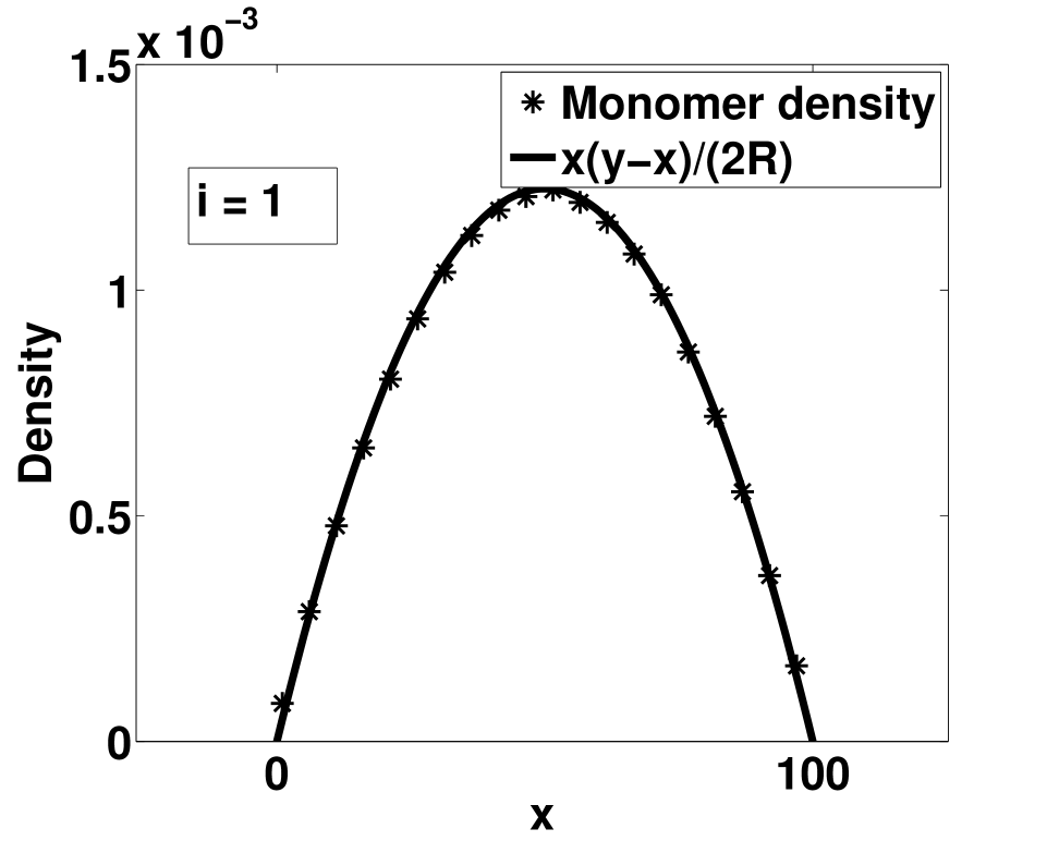
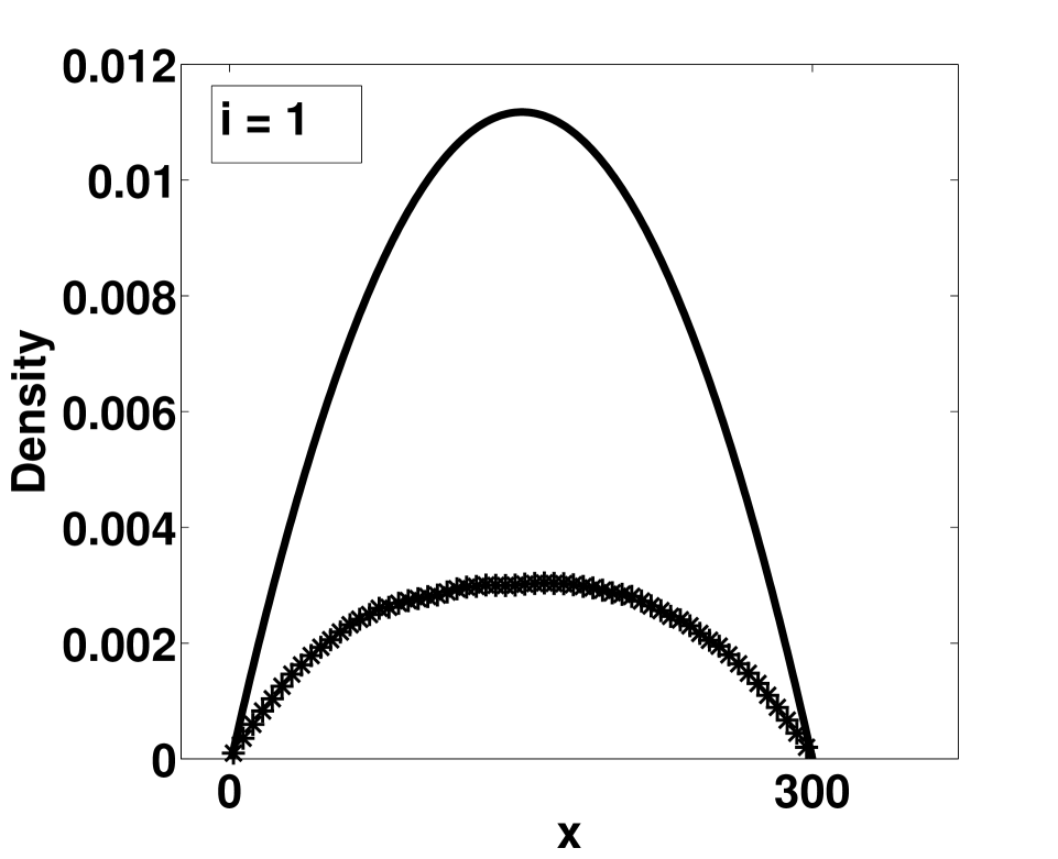
Figure 2: Monomer density profile in a single gap of size $g=100$ (top) and $g=300$ (bottom) for $i=1$

In Fig. 3 we show the average time for a nucleation event to occur $\langle t_{nuc}\rangle$ for all single gaps in the case of $i=1$, $2$ and $3$ (note that the data for $i=2$ and $i=3$ have been shifted horizontally to avoid overlapping curves). We note that the data obeys the power-law form predicted by the fragmentation equation approach for small gap sizes $g$, but as expected deviates strongly for larger gaps. In fact, the average time to nucleation becomes much higher than predicted by the use of the saturated monomer density profile, since the actual profile for the larger gaps is lower, therefore presenting slower than expected nucleation rates (but still fast compared to the time it takes for the monomer density to grow from zero to its saturation level).

The straight line fits in Fig. 3 are for the small gap size data only ($g\in[50,150]$). We use these to estimate how the nucleation rate varies with gap size $g$ through $1/\langle t_{nuc}\rangle\propto g^{\gamma}$, with the values of the power $\gamma$ reported in Table 1. We have used bootstrap methods with $1000$ samples of size as big as $80$% of the original to find an approximate $95\%$ confidence interval in Table 1.

The fragmentation equation approach (Section IIA above) suggests that this power should be $2i+1$ or $2i+3$, depending on whether island nucleation is driven by monomer deposition or solely by monomer diffusion. The results in Table 1 suggest that the simulation reflects both these mechanisms, with the small gap size nucleation rate exponent lying between these two possibilities.

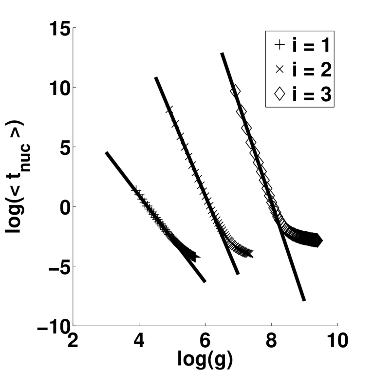
Figure 3: Average time for a nucleation event to occur at all gaps.

$i$	$\lambda$	$\lambda$	Simulation
$1$	$3$	$5$	$3.628\pm 0.035$
$2$	$5$	$7$	$6.606\pm 0.118$
$3$	$7$	$9$	$8.283\pm 0.266$

Table 1: Small gap nucleation rate exponents from the single gap simulations.

In Fig. 4 we present histograms for the number of hops taken by the youngest monomer in a nucleus for the $g=100$ and $g=300$ $i=1$ simulations. The histogram has a long tail, showing that in many cases all the monomers in the nucleus are indeed mature in the sense that they have diffused many times since their deposition. However, there is also a sharp increase in likelihood of a monomer only taking very few diffusive steps before being caught up in a nucleation event. In other words, there are a significant number of nucleation events driven by fluctuations due to deposition. This supports the conclusion that nucleation in these simulations is driven by a combination of deposition and diffusion fluctuations in monomer density, helping to explain the intermediate values for the nucleation rate exponents in Table 1.

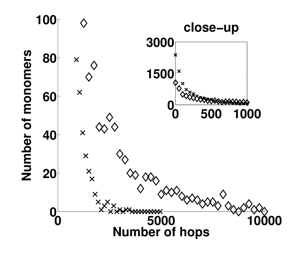
Figure 4: Histogram of the number of hops taken by the youngest monomer in a nucleus for $i=1$, for gap size $g=100$ (crosses) and $g=300$ (diamonds). In the main figure the number of monomers is truncated at $100$. The inset shows the same result at the lower number of hops without truncation of the number of monomers in the histogram.

IV.2 FULL SIMULATION BEHAVIOUR

Having established the nucleation behaviour in single gaps, we can now look at the results observed in our full Monte Carlo simulations. The fragmentation equation approach again provides concrete predictions for the small and large size behaviours for the GSD and CZD. We will also be able to compare the CZD properties with the GWS, and establish which of the two theories provides the better framework to understand the behaviour observed.

IV.2.1 SMALL SIZE SCALING OF THE GSD AND CZD

In Figures 5 and 6, we report the small size behaviour of the GSD ($\phi(z)$) and CZD ($P(s)$) in logarithmic scale at $\theta=20$%. In order to fit the slopes in these plots, and obtain reliable error estimates, we adopt the following numerical technique. The size data are binned using regularly spaced bins on the logarithmic abscissa, with bin widths $b^{m}c$ where $b$ and $c$ are fixed constants and $m\geq 0$. By choosing a range of values for $b=1.1$, $1.2$, $1.3$ and $1.4$, and $c=0.0125$, $0.025$ and $0.05$, all of which provide reasonable choices for binning the data, we obtain a number of straight-line fits. This allows us to calculate the average of these gradients and a $95$% confidence interval. The results of this fitting procedure are shown in Tables 2 and 3.

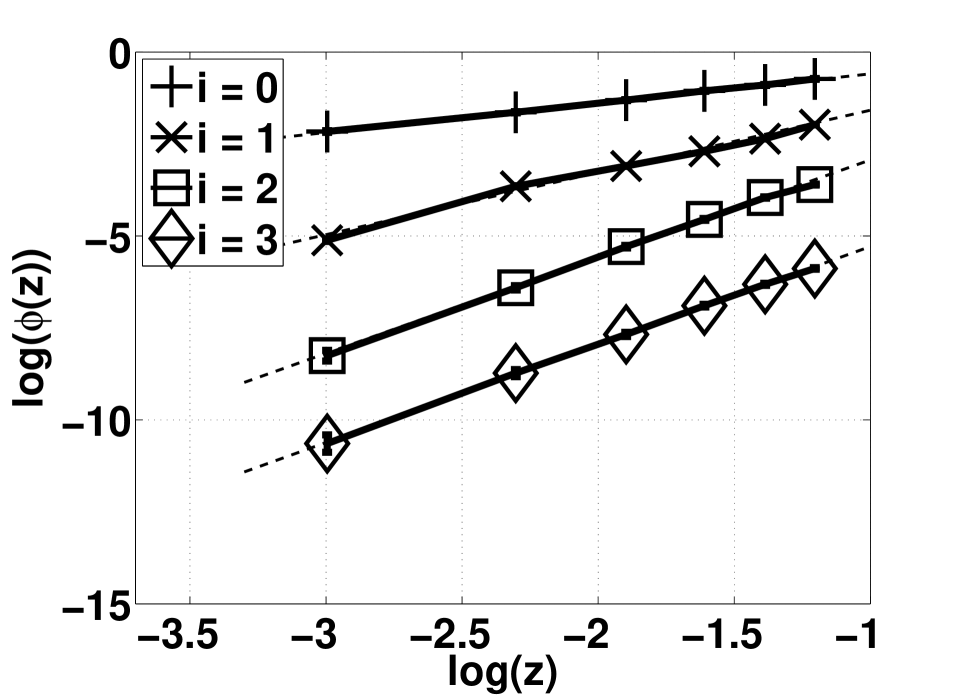
Figure 5: Small-size GSD in logarithmic scale for $i=0$, $1$, $2$ and $3$ at coverage $\theta=20$%. The dashed line is the straight line fit to data.

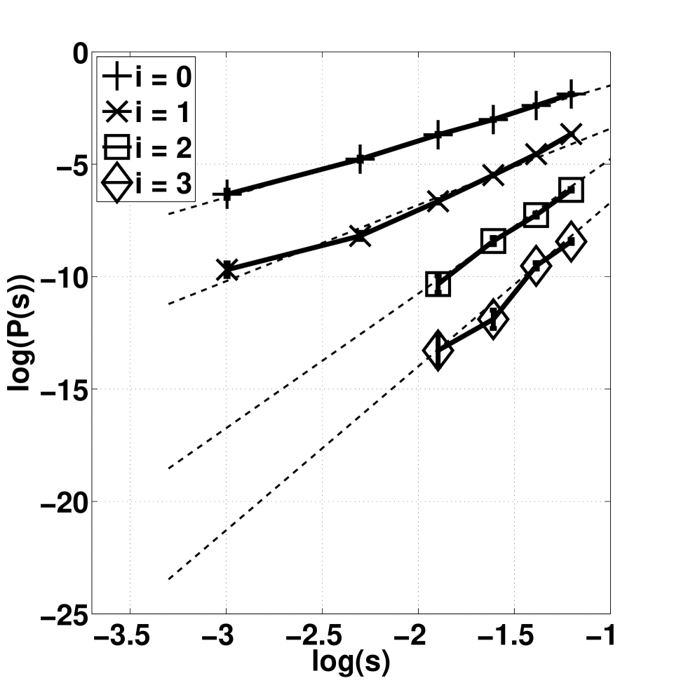
Figure 6: Small-size CZD in logarithmic scale for $i=0$, $1$, $2$ and $3$ at coverage $\theta=20$%. The dashed line is the straight line fit to data.

For the small-size asymptotic behaviour of the GSD and CZD we compare the data from MC simulations with the fragmentation equation approach predictions of Section IIA. For the GSD, the dominant term is $z^{\alpha}$ as $z\rightarrow 0$ (see Eqn. (4)). Likewise, for the CZD the dominant term is $s^{2\alpha+1}$ (see Eqn. (7)). For the latter, we also have the competing prediction of the GWS which is $s^{\beta}$ (Eqn. (9)). The values from these theories are also displayed in Tables 2 and 3.

$i$	$\alpha$	$\alpha$	GSD	GSD
$0$	-	$1$	$0.876\pm 0.033$	$0.905\pm 0.029$
$1$	$1$	$2$	$1.701\pm 0.045$	$1.579\pm 0.105$
$2$	$2$	$3$	$2.789\pm 0.080$	$2.718\pm 0.074$
$3$	$3$	$4$	$2.719\pm 0.082$	$3.271\pm 0.056$

Table 2: Average gradient for the small size scaling of the GSD using different bin-widths at coverage $\theta=20$% and $100$%

$i$	$2\alpha+1$	$2\alpha+1$	GWS	CZD	CZD
$0$	-	$3$	$2$	$2.730\pm 0.030$	$2.751\pm 0.086$
$1$	$3$	$5$	$4$	$4.187\pm 0.050$	$4.372\pm 0.149$
$2$	$5$	$7$	$6$	$5.883\pm 0.207$	$5.957\pm 0.187$
$3$	$7$	$9$	$8$	$7.200\pm 0.382$	$6.138\pm 0.124$

Table 3: Average gradient for the small size scaling of the CZD using different bin-widths at coverage $\theta=20$% and $100$%

The results for the small size scaling exponent of the GSD in Table 2 show that the fragmentation equation approach provides a reasonably sound framework for understanding the island nucleation and growth process. For $i=1,2,3$ we see that the exponent at $\theta=100$% lies between the two possible values $\alpha=i$ and $\alpha=i+1$ suggested by the theory. This is as expected following the single-gap nucleation results presented above, which show that both the deposition- and diffusion-driven nucleation mechanisms are at play in the simulations. We note that the $\theta=20$% results for $i=3$ lie below $\alpha=i=3$, but we believe that this is due to the fact that the simulation has only just entered the aggregation regime in this case. We also see that for $i=0$, the exponent is close to the $\alpha=i+1=1$ prediction ($\alpha=0$ is not a viable possibility), being closer at $\theta=100$%.

The trends shown in the small size scaling exponent of the CZD in Table 3 are rather similar. We see the $i=0$ data are close to the $\lambda=2i+3=3$ prediction of the fragmentation equation approach, being somewhat larger than the $\beta=2(i+1)=2$ predicted by the GWS. For $i=1,2$ the data are bracketed by the two alternatives suggested by the fragmentation theory, as indeed is the GWS exponent which appears to present a reasonable compromise given the two alternative nucleation mechanisms. The case of $i=3$ provides an exception, which hints at the breakdown of the relation in Eqn. (6) between the GSD and the CZD. This will be discussed further in the final section.

IV.2.2 LARGE SIZE SCALING OF THE GSD AND CZD

In Figures 7 and 8 we present the large-size behaviour of the GSD and CZD from the full simulations. The data are plotted in order to test the common large-size functional form suggested by the fragmentation equation approach for the GSD and by the GWS for the CZD , namely $\exp(-cz^{p})$ (see Eqns. (5) and (9)). In all cases, the data do conform well to this functional form. In addition, we perfom fits to find the gradients $p$ on these plots. In order to provide an estimate of the error in these fits, we adopt a similar strategy to that used above for the small-size scaling and bin the data using binwidths of size $0.01k$ with $k=1,2,...,20$. The results of this fitting procedure are presented in Tables 4 and 5 for the GSD and CZD respectively.

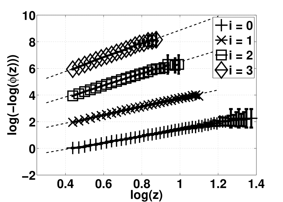
Figure 7: Large-size GSD in logarithmic scale for $i=0$, $1$, $2$ and $3$. The dashed line is the straight line fit to data.

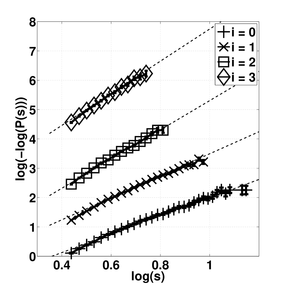
Figure 8: Large-size CZD in logarithmic scale for $i=0$, $1$, $2$ and $3$. The dashed line is the straight line fit to data.

Once again we compare the exponents $p$ from the Monte Carlo simulation data with the theoretical predictions. For the GSD, the fragmentation equation approach predicts values of $2\alpha+1$ for $p$. For the CZD, the fragmentation equation prediction is $p=3$ for $i=0$ (Eqn. (8)) and we conjecture that the values for $i>0$ will match those of the GSD. In contrast, the GWS prediction for the CZD is the universal value $p=2$. The values from these theories are displayed in Tables 4 and 5.

$i$	$2\alpha+1$	$2\alpha+1$	GSD	GSD
$0$	-	$3$	$2.515\pm 0.006$	$2.665\pm 0.007$
$1$	$3$	$5$	$3.130\pm 0.009$	$3.383\pm 0.008$
$2$	$5$	$7$	$4.364\pm 0.020$	$5.112\pm 0.025$
$3$	$7$	$9$	$5.094\pm 0.026$	$6.437\pm 0.034$

Table 4: Average exponents for the large size scaling of the GSD using different bin-widths at coverage $\theta=20$% and $100$%

$i$	$2i+3$	GWS	CZD	CZD
$0$	$3$	$2$	$3.108\pm 0.012$	$3.043\pm 0.043$
$1$	-	$2$	$3.721\pm 0.020$	$3.826\pm 0.021$
$2$	-	$2$	$4.946\pm 0.029$	$5.536\pm 0.033$
$3$	-	$2$	$5.464\pm 0.041$	$6.530\pm 0.042$

Table 5: Average exponents for the large size scaling of the CZD using different bin-widths at coverage $\theta=20$% and $100$%

In Table 4 we see that the fragmentation equation approach provides a useful point of reference to the observed large-size scaling exponents of the GSD. Again we see values that are bracketed by the two possible nucleation mechanisms for $i=1,2$, whilst the behaviour for $i=0$ is a little below the predicted exponent of $p=3$. For $i=3$ the data’s exponent is below even that of the deposition-induced nucleation case. However, we have shown in Section III above that the monomer density profile does not reach its saturation value in larger gaps, so that the nucleation rate in these gaps is lower than predicted by the theory. This seems to provide a rational explanation for the discrepancies.

The results in Table 5 for the large-size scaling behaviour of the CZD are rather informative. We firstly observe that the Monte Carlo data exponents do indeed mirror those of the GSD in Table 4 quite well. This means that the universal GWS prediction for $p=2$ is always wrong. We also see that the concrete prediction for $i=0$ from the fragmentation equations, namely $p=3$, is well supported by the simulation data.

V SUMMARY AND CONCLUSIONS

We have investigated one-dimensional (1-D) point island nucleation and growth simulations in order to test predictions for the asymptotics of the gap and capture zone size distributions (GSD and CZD respectively). The work shows that the fragmentation equation approach provides a good framework in which to understand the Monte Carlo simulation results. The theory can be used to investigate two cases for the nucleation process for $i>0$, the first where nucleation is driven by deposition events, the second where fluctuations caused solely by monomer diffusion induce nucleation.

Firstly we presented single gap simulation results which show that both these nucleation processes are active, so that the observed nucleation rates are bracketed by these two extremes. Furthermore, we showed that for larger gaps the average monomer density profile does not reach the long-time steady state assumed in the fragmentation equations. As a result, the nucleation rates in large gaps are slower than predicted by the theory, with the shortfall increasing with gap size. Therefore, the simple power-law scaling of the nucleation rate with gap size breaks down at larger sizes, with obvious consequences for the fragmentation equation predictions for the GSD.

We note here that deviations from the original Blackman and Mulheran BM96 predictions for the nucleation rate dependence on gap size have recently been observed for the $i=1$ 1-D model GPE11 . In this work, the authors report that the nucleation rate has two regimes; for small sizes, it approximately obeys $s^{4}$, whilst at larger sizes it approximately follows $s^{3}$. The latter power-law feeds into the asymptotic form of the GSD and hence the CZD, yielding the functional form $\exp(-s^{3})$. We note here that these values are close to those we find for $i=1$ in Table 1 for the small gap nucleation rates and Tables 4 and 5 for the large-size GSD and CZD scaling. We therefore propose that the explanations presented here in terms of competing nucleation mechanisms and unsaturated monomer density profiles will also explain the results reported in [GPE11, ].

We also presented data for the full island nucleation and growth simulation. For the small-size GSD scaling, we found results consistent with the fragmentation equation predictions for $i=0$. For $i=1,2,3$ the exponents were bracketed by the values for the alternative nucleation mechanisms as expected. For the large gap size scaling, the Monte Carlo data followed the functional form suggested by the fragmentation theory, with the exponents again being largely bracketed by the predicted values, although the breakdown of the nucleation rate scaling is apparent, especially for larger $i$.

In the case of the CZD, we once again successfully placed the observed simulation data into the context provided by the fragmentation equations. Interestingly, the GWS predictions for the small-size CZD scaling work extremely well since they bisect the exponents from the alternative nucleation mechanisms. As discussed elsewhere GLOM11 , the predicted formula for the parameter $\beta$ of the GWS can be brought into line with either nucleation mechanism following the arguments of Pimpinelli and Einstein PE10 , but the original prediction of these authors (Eqn. (10)) does seem to speak well for their physical intuition PE07 .

However, the predicted GWS form for the large-size CZD scaling fails badly when confronted with our 1-D point island simulation results. This is in contrast to recent tests performed using two-dimensional substrates Oliv11 , which suggests that there is something unique to the 1-D case, possibly due to the topological constraints in how capture zones are constructed from the inter-island gaps. This aspect is worthy of further investigation.

In order to predict the asymptotics of the CZD, we have assumed that the capture zones can be constructed from pairs of gaps sampled randomly for the GSD (see Eqn. (6)). This is valid provided that the nucleation has effectively mixed up the gaps so that nearest neighbours are no longer correlated BM96 . One consequence is that the small-size exponents of the CZD (say $p_{1}$) are related to those of the GSD (say $p_{2}$) through $p_{1}=2p_{2}+1$. Looking at the results in Tables 2 and 3, we see that this relationship is reasonably obeyed for $i=0,1$ but starts to break down for $i=2,3$. This is perhaps understandable, since for the higher critical island sizes, the nucleation rate slows down dramatically over time suggesting less well-mixed systems. This is another point for further consideration in future theory development work.

Despite the limitations of the fragmentation equation approach used in this work, such as its failure to capture the time-dependent nature of the monomer density profile within gaps, it has provided an excellent theoretical framework from which to consider the island nucleation process. Hence, alongside the points discussed above, future work might also look at how the fragmentation kernels can incorporate this time dependency, and how the two nucleation mechanisms can be combined into a consistent set of fragmentation equations.

http://www.mathstat.strath.ac.uk/

http://www.strath.ac.uk/chemeng/research
/groupdetails/drpaulmulheran-seniorlecturer/

References

- (1) A. -L. Barabási and H. E. Stanley, Fractal Concepts in Surface Growth, Cambridge University Press, Cambridge 1995.
- (2) J. A. Venables, G. D. T. Spiller and M. Hanbücken, Rep. Prog. Phys. 47 399 (1984).
- (3) J. G. Amar, M. N. Popescu and F. Family, Phys. Rev. Lett. 86 3092 (2001).
- (4) P. A. Mulheran, D. Pellenc, R. A. Bennett, R. J. Green and M. Sperrin, Phys. Rev. Lett 100 068102 (2008).
- (5) P. A. Mulheran, Theory of Cluster Growth on Surfaces, in: ISSN 1570-002X, Handbook of Metal Physics, Elsevier B.V. 2009, 73–111.
- (6) J. W. Evans, P. A. Thiel and M. C. Bartelt, Sur. Sci. Rep. 61 1 (2006).
- (7) P. A. Mulheran and J. A. Blackman, Philos. Mag. Lett. 72 55 (1995).
- (8) P. A. Mulheran and J. A. Blackman, Phys. Rev. B 53 10261 (1996).
- (9) M. C. Bartelt, A. K. Schmid, J. W. Evans and R. Q. Hwang, Phys. Rev. Lett. 81 1901 (1998).
- (10) P. A. Mulheran and D. A. Robbie, Europhys. Lett. 49 617 (2000).
- (11) J. W. Evans and M. C. Bartelt, Phys. Rev. B 66 235410 (2002).
- (12) P. A. Mulheran, Europhys. Lett. 65 379 (2004).
- (13) A. Pimpinelli and T. L. Einstein, Phys. Rev. Lett 99, 226102 (2007).
- (14) M. Li, Y. Han and J. W. Evans, Phys. Rev. Lett. 104 149601 (2010).
- (15) A. Pimpinelli and T. L. Einstein, Phys. Rev. Lett. 104 149602 (2010).
- (16) F. Shi, Y. Shim and J. G. Amar, Phys. Rev. E 79 011602 (2009).
- (17) T. J. Oliveira and F. D. A. Aarao Reis, Phys. Rev. B 83 201405 (2011).
- (18) V. I. Tokar and H. Dreyssé, Phys. Rev. E 77 066706 (2008).
- (19) J. A. Blackman and P. A. Mulheran, Phys. Rev. B 54 11681 (1996).
- (20) M. Grinfeld, W. Lamb, K. P. O’Neill and P. A. Mulheran, J. Phys. A 45 015002 (2012).
- (21) D. L. González, A. Pimpinelli and T. L. Einstein, Phys. Rev. E 84 011601 (2011).
- (22) R. M. Ziff and E. D. McGrady, Marcomolecules 19 2513 (1986).
- (23) Z. Cheng and S. Redner, Phys. Rev. Lett. 60 2450 (1988).
- (24) M. Escobedo, S. Mischler, M. Rodriguez Ricard, Ann. Inst. H. Poincaré Anal. Non Linéaire 22 99 (2005).
- (25) J. G. Amar, F. Family and P.-M. Lam, Phys. Rev. B 50 8781 (1994).
- (26) C. Ratsch, Y. Landa and R. Vardavas, Surf. Sci. 578 196 (2005).