The fluctuating $\alpha$-effect and Waldmeier relations in the nonlinear dynamo models

Abstract

We study the possibility to reproduce the statistical relations of the sunspot activity cycle, like the so-called Waldmeier relations, the cycle period - amplitude and the cycle rise rate - amplitude relations, by means of the mean field dynamo models with the fluctuating $\alpha$-effect. The dynamo model includes the long-term fluctuations of the $\alpha$-effect and two types of the nonlinear feedback of the mean-field on the $\alpha$-effect including the algebraic quenching and the dynamic quenching due to the magnetic helicity generation. We found that the models are able to reproduce qualitatively and quantitatively the inclination and dispersion across the Waldmeier relations with the 20% fluctuations of the $\alpha$-effect. The models with the dynamic quenching are in a better agreement with observations than the models with the algebraic $\alpha$-quenching. We compare the statistical distributions of the modeled parameters, like the amplitude, period, the rise and decay rates of the sunspot cycles, with observations.

1 Introduction

It is observed that the sunspot’s activity is organized in time and latitude and forms the large scales patterns which are called the Maunder butterfly diagram. This pattern is believed to be produced by the large-scale toroidal magnetic field generated in the convection zone. Another component of the solar activity is represented by the global poloidal magnetic field extending outside the Sun and shaping the solar corona. Both components synchronously evolve as the solar 11-year cycle progresses. The global poloidal field reverses the sign in the polar regions near the time of maximum of sunspot activity.

A remarkable feature of cyclic solar activity is that it is far to be just a cycle. Cycle amplitude and shape varies from one cycle to the other and prognostic abilities of any study of solar activity looks as its very attractive destination. Solar activity observations give various hints that various tracers of solar activity which are exploited to quantify the phenomenon demonstrate some relation one to the other what opens a possibility to predict future evolution of solar activity basing on available observations of other indices. Waldmeier [36] pointed out at first this option (an inverse correlation between the length of the ascending phase of a cycle, or its "rise time", and the peak sunspot number of that cycle) and applied it, [37], to give a prediction for the following cycle. The latter paper is in practice the first accessible (at least for German speaking readers) paper in the area. Later other relation of this this type was suggested and summarized as Waldmeier relations. This development was clearly summarized by [35] and recently by [12]. The nature of the physical processes, that are manifested in the Waldmeier relations, is not clear, see discussion, e.g., in [6, 10, 8]. It seems to be remarkable, however, that these statistical properties of magnetic activity are also existed for the other tracers related with the sunspot activity (e.g., sunspot group and squares of sunspot groups, see [35, 12, 8]), and even for the other kind of the solar and stellar activity indices, e.g., for the Ca II index [31]. The Waldmeier relations are considered as a valuable test of the dynamo models [15, 8, 29].

A natural way to push the understanding of the problem forward is to clarify the physics underlying Waldmeier relations. It is more or less accepted that cyclic solar activity is driven by a dynamo, i.e. a mechanism which transforms kinetic energy of hydrodynamical motions into magnetic one. Most of the current solar dynamo models suggest that the toroidal magnetic field that emerges on the surface and forms sunspots is generated near the bottom of the convection zone, in the tachocline or just beneath it in a convection overshoot layer (see, e.g., [32]). This kind of dynamo can be approximated by the Parker’s surface dynamo waves [26]. The direction of the dynamo waves propagation is defined by the Parker-Yoshimura rule [38]. It states that for the $\alpha\Omega$ kind dynamo the waves propagates along iso-surfaces of the angular velocity. The propagation process can be modified by the turbulent transport (associated with the mean drift of magnetic activity in the turbulent media by means turbulent mechanisms), by the anisotropic turbulent diffusivity (see, [14]), and by meridional circulation [7]. A viewpoint, which is an alternative to the Parker’s surface dynamo waves is presented by the distributed dynamo with subsurface shear, e.g. [3]. The dynamo waves here propagates along the radius in the main part of the solar convection zone, [14]. The near surface activity is shaped by the subsurface shear. One more option is the flux-transport dynamo, e.g. [7, 9].

In the context of dynamo theory, the Waldmeier relations have to be explained by some mechanism which varies amplitude and shape of activity cycle and fluctuations $\alpha$-effect are considered below as such mechanism. This idea extend the approach proposed in [29] to explain these relations by changing the magnitude of the $\alpha$-effect.

The physical idea underlying this mechanism can be presented as follows. $\alpha$-coefficient is a mean quantity taken over ensemble of convective vortexes. Number $N$ of the vortexes in solar convective shell is large however much smaller then, say, the Avogardo number, so fluctuations being proportional to $N^{-1/2}$ may be not negligible. Particular choice of $N$ is obviously model dependent however if we take just for orientation $N=10^{4}$ then $N^{-1/2}=0.01$. Taking into account that $\alpha$ is usually about 1/10 of turbulent velocity we consider a dozen percent of $\alpha$-fluctuations as a comfortable estimate. From the other hand, governing equations for large-scale solar magnetic field deal with spatial averaging and have to include a contribution of $\alpha$-fluctuations, [13].

A straightforward application of the idea with vortex turnover time and vortex size as correlation time and length for $\alpha$-fluctuations needs fluctuations much larger then mean $\alpha$. [24], [34] based on experiences in direct numerical simulations, e.g. [4], and results of current helicity (related to $\alpha$) observation in solar active regions, e.g. [39] considered $\alpha$-fluctuations with correlation time comparable with cycle length and correlation length comparable with the extent of the latitudinal belts where sunspots occur to conclude that a reasonable $\alpha$-noise of order of few dozen percents is sufficient to explain Grand minima of solar activity. The aim of this paper is to apply this idea to explain Waldmeier relations.

2 Basic equations

2.1 2D model

The dynamo model is based on the standard mean-field induction equation in perfectly conductive media [19]:

$$\frac{\partial\mathbf{B}}{\partial t}=\boldsymbol{\nabla}\times\left(\mathbf{\boldsymbol{\mathcal{E}}+}\mathbf{U}\times\mathbf{B}\right)$$

where $\boldsymbol{\mathcal{E}}=\overline{\mathbf{u\times b}}$ is the mean electromotive force, with $\mathbf{u,\,b}$ being the turbulent fluctuating velocity and magnetic field respectively; $\mathbf{U}$ is the mean velocity (differential rotation). The axisymmetric magnetic filed:

$$\mathbf{B}=\mathbf{e}_{\phi}B+\nabla\times\frac{A\mathbf{e}_{\phi}}{r\sin\theta}$$

$\theta$ - polar angle. We have used the expression for $\boldsymbol{\mathcal{E}}$ obtained by [27] (hereafter P08) and write it as follows:

$$\mathcal{E}_{i}=\left(\alpha_{ij}+\gamma_{ij}\right)\overline{B}_{j}-\eta_{ijk}\nabla_{j}\overline{B}_{k}.$$ (1)

Tensor $\alpha_{i,j}$ represents the alpha effect, including the hydrodynamic and magnetic helicity contributions,

$$\alpha_{ij}=C_{\alpha}\left(1+\xi\right)\psi_{\alpha}(\beta)\sin^{2}\theta\alpha_{ij}^{(H)}+\alpha_{ij}^{(M)},$$ (2)

where the hydrodynamical part of the $\alpha$-effect, $\alpha_{ij}^{(H)}$, $\xi$ is the noise, and the quenching function, $\psi_{\alpha}$, are given in Appendix (see also in [28]). The hydrodynamic $\alpha$-effect term is multiplied by $\sin^{2}\theta$ ($\theta$ is co-latitude) to prevent the turbulent generation of magnetic field at the poles. The contribution of the small-scale magnetic helicity $\overline{\chi}=\overline{\mathbf{a\cdot}\mathbf{b}}$ ($\mathbf{a}$ is a fluctuating vector-potential of magnetic field) to the $\alpha$-effect is defined as $\alpha_{ij}^{(M)}=C_{ij}^{(\chi)}\overline{\chi}$, where coefficient $C_{ij}^{(\chi)}$ depends on the turbulent properties and rotation, and is given in Appendix. The other parts of Eq.(1) represent the effects of turbulent pumping, $\gamma_{ij}$, and turbulent diffusion, $\eta_{ijk}$. They are the same as in PK11. We describe them in Appendix.

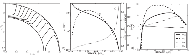
Figure 1: Parameters of the solar convection zone: a) the contours of the constant angular velocity plotted for the levels $(0.75-1.05)\Omega_{0}$ with a step of $0.025\Omega_{0}$, $\Omega_{0}=2.86\cdot 10^{-7}s^{-1}$; b) turnover convection time $\tau_{c}$, and the RMS convective velocity $u^{\prime}_{c}$ and the background turbulent diffusivity $\eta_{T}^{(0)}$ profiles; c) the radial profiles of the $\alpha$-effect tensor components.

The nonlinear feedback of the large-scale magnetic field to the $\alpha$-effect is described as a combination of an “algebraic” quenching by function $\psi_{\alpha}\left(\beta\right)$ (see Appendix and [29]), and a dynamical quenching due to the magnetic helicity conservation constraint. The magnetic helicity, $\overline{\chi}$ , subject to a conservation law, is described by the following equation [18, 5, 33]:

$$\frac{\partial\overline{\chi}}{\partial t} = -2\left(\boldsymbol{\mathcal{E}\cdot}\overline{\mathbf{B}}\right)-\frac{\overline{\chi}}{R_{\chi}\tau_{c}}+\boldsymbol{\nabla}\cdot\left(\eta_{\chi}\boldsymbol{\nabla}\bar{\chi}\right),$$ (3)

where $\tau_{c}$ is a typical convection turnover time. Parameter $R_{\chi}$ controls the helicity dissipation rate without specifying the nature of the loss. It seems to be reasonable that the helicity dissipation is most efficient in the near surface layers because of the strong decrease of $\tau_{c}$ (see Figure 1b). The last term in Eq.(3) describes the diffusive flux of magnetic helicity [20]. We use the solar convection zone model computed by [32], in which the mixing-length is defined as $\ell=\alpha_{MLT}\left|\Lambda^{(p)}\right|^{-1}$, where $\mathbf{\boldsymbol{\Lambda}}^{(p)}=\boldsymbol{\nabla}\log\overline{p}\,$ is the pressure variation scale, and $\alpha_{MLT}=2$. The turbulent diffusivity is parametrized in the form, $\eta_{T}=C_{\eta}\eta_{T}^{(0)}$, where $\eta_{T}^{(0)}={\displaystyle\frac{u^{\prime}\ell}{3}}$ is the characteristic mixing-length turbulent diffusivity, $\ell$ and $u^{\prime}$ are the typical correlation length and RMS convective velocity of turbulent flows, respectively and $C_{\eta}$ is a constant to control the intensity of turbulent mixing. In the paper we use $C_{\eta}=0.05$. The differential rotation profile, $\Omega=\Omega_{0}f_{\Omega}\left(x,\mu\right)$, $x=r/R_{\odot}$, $\mu=\cos\theta$ is a modified version of an analytical approximation to helioseismology data, proposed by [2], see Fig. 1a.

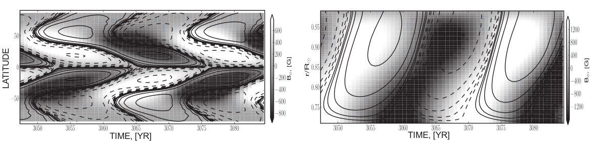
Figure 2: The typical time-latitude and the time-radius (at the $30^{\circ}$ latitude) diagrams of the toroidal field (grey scale), the radial field (contours at left panel) and the poloidal magnetic field (contours at the right panel) evolution in 2D1 model (see Table 1). The toroidal field averaged over over the subsurface layers in the range of $0.9-0.99R_{\odot}$ , the radial field is taken at the top of the convection zone.

We use the standard boundary conditions to match the potential field outside and the perfect conductivity at the bottom boundary. As discussed above, the penetration of the toroidal magnetic field in to the near surface layers is controlled by the turbulent diffusivity and pumping effect. For magnetic helicity, similar to [11] and [21], we use the time dependent conditions provided be Eq.3 and the helicity flux conservation the condition $\boldsymbol{\nabla_{r}}\bar{\chi}=0$ is applied at the bottom and at the top of domain. The latter gives a smooth transfer for solutions with and without the diffusive helicity flux.

The left panel on the Fig. 2 shows the typical the time-latitude diagram for the toroidal magnetic averaged over the subsurface layers $0.9-0.99R_{\odot}$ and the radial magnetic at the top of the integration domain. The right panel shows the time-radius the time-radius diagram for the toroidal an poloidal magnetic field evolution at $30^{\circ}$ latitude.

We demonstrate it by Fig. 3 which shows the time-latitude diagrams for toroidal and radial magnetic field evolution for the models 1D1, 1D3 and 2D1. For the latter model we show the toroidal magnetic averaged over the subsurface layers $0.9-0.99R_{\odot}$ and the radial magnetic field is given for the top of the integration domain. For the model 2D1 we show the time-radius diagram for the toroidal an poloidal magnetic field evolution at $30^{\circ}$ latitude. The other models listed in Table 1, having the same general patterns of the magnetic field evolution, are differed from the models shown on the Fig. 3 in some details (mostly associated with magnetic helicity evolution).

2.2 1D model

For comparison with the previous studies and also to study how the additional dimension affect the statistical properties of the dynamo we consider the $1D$ model similar to that studied by [24]:

$$\frac{\partial A}{\partial t} = \sin\theta\left(\left(1+\xi\right)\cos\theta\psi_{\alpha}(B)+\chi\right)B+\sin\theta\frac{\partial}{\partial\theta}\left(\frac{1}{\sin\theta}\frac{\partial A}{\partial\theta}\right)-\eta_{CZ}A,$$ (4)

$$\frac{\partial B}{\partial t} = -\mathcal{D}\tilde{\Omega}\left(\theta\right)\frac{\partial A}{\partial\theta}+\frac{\partial}{\partial\theta}\left(\frac{1}{\sin\theta}\frac{\partial\sin\theta B}{\partial\theta}\right)-\eta_{CZ}B,$$ (5)

where the large-scale radial shear $\tilde{\Omega}\left(\theta\right)=\partial\Omega/\partial r$. The $1D$ model employs two possibilities for the shear profile. In one case we put $\tilde{\Omega}\left(\theta\right)=1$, that give us the model explored by [24]. In another case we use

$$\tilde{\Omega}=\frac{1}{10}\left(5\sin^{2}\theta-4\right),$$ (6)

which is suggested by [16]. In agreement with the helioseismology results for the bottom of the convection zone, this profile is positive in equatorial regions and negative near the poles. The magnetic field strength in Eq.(5) is measured in the units of the equipartition magnetic field strength and the time is normalized to the typical diffusive time, $R_{\odot}^{2}/\eta_{T}^{(0)}$. The evolution of the magnetic helicity for the 1D model is governed by equation:

$$\frac{\partial\overline{\chi}}{\partial t} = -2\left((1+\xi)\cos\theta\psi_{\alpha}(B)+\chi\right)B^{2}-2B\frac{\partial}{\partial\theta}\left(\frac{1}{\sin\theta}\frac{\partial A}{\partial\theta}\right)$$

$$+ \frac{2}{\sin^{2}\theta}\frac{\partial A}{\partial\theta}\frac{\partial\sin\theta B}{\partial\theta}-\frac{\overline{\chi}}{R_{\chi}}+\frac{\eta_{\chi}}{\sin\theta}\frac{\partial}{\partial\theta}\left(\frac{1}{\sin\theta}\frac{\partial\bar{\chi}}{\partial\theta}\right).$$

In what follows we will discuss the 1D models with the constant shear, because they are more relevant to compare with observations. The differences in results for the 1D models with the variable shear given by Eq.(6) will be briefly mentioned in subsequent sections.

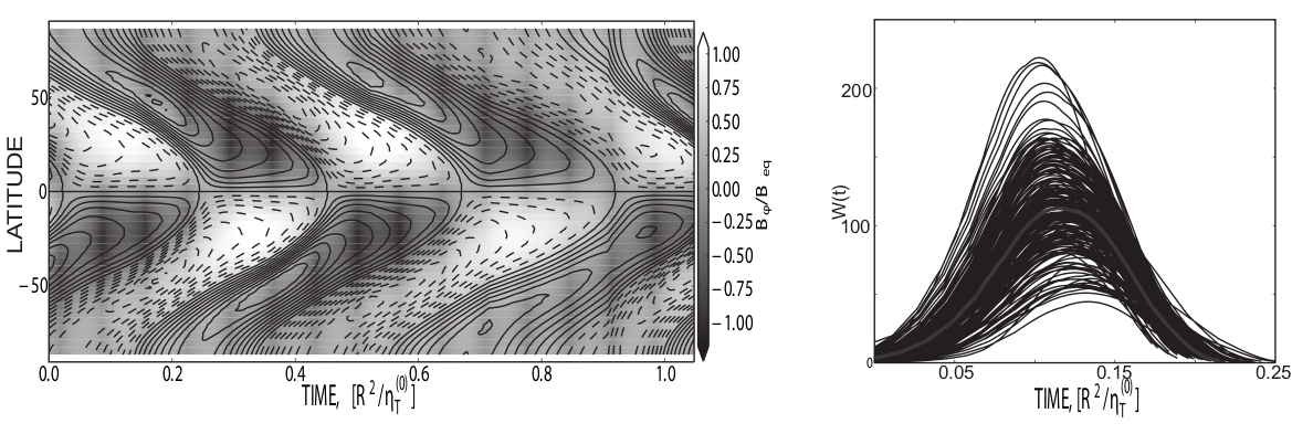
Figure 3: The left panel shows the time-latitude diagrams of the toroidal field (grey scale) and the radial field (contours) for the 1D1 model (see Table 1). The right panel shows the estimated sunspot number in the the separated cycles in the 1D1 model (see Section 2.4).

Summarizing, we exploit much more detailed and realistic dynamo models then [24], [34]. Our point is that Waldmeier relations are a much more delicate phenomena rather Grand minima and the bulk of our knowledge concerning recent solar cycles is much more rich then that one for remote past when Grand minima took place.

2.3 Noise model

The noise, $\xi$, contributes in the hydrodynamic part of the $\alpha$-effect (see, Eqs.(2,4)). Following to [34] the models employ the long-term Gaussian fluctuating $\xi$ of the small amplitude with RMS deviation given in the Table 1 (last column). The time of the renewal of the $\xi$ is equal to the period of the model. The random numbers were generated with help of the standard F90 subroutine quality of contemporary standard noise generator subroutine is shown to be sufficient for such kind of modelling, see e.g. [1]). It would be more realistic to consider the renewal time as the fluctuating quantity as well, but we would like to separate this effect for the different study. Also, we found that the models which employ the magnetic helicity effect show the very intermittent long term behaviour. This makes the analysis procedure (e.g., division to subsequent cycles) more complicated. We isolate ourselves from these phenomena by considering the noise models with the lower RMS in case if the magnetic helicity is employed.

Model	$\eta_{CZ}$	$\overline{\chi}$	$\eta_{\chi}/\eta_{T}$	$R_{\chi}$	$B_{0}$	$C_{W}$	$\sigma$
1D1	1	0	0	10	3	1200	0.15
2D1		Eq.(2)	$10^{-5}$	200	800	1	0.15
2D2		Eq.(2)	$0.3$	$10^{6}$	200	1	0.15

Table 1: Parameters the dynamo models: the type of the nonlinear quenching of the $\alpha$-effect, if the magnetic helicity is $\overline{\chi}=0$ then the model employ only the algebraic quenching which is described by $\psi_{\alpha}$and otherwise by the dynamic quenching due to magnetic helicity described by Eq.(3) or Eq.(2.2); $\eta_{\chi}/\eta_{T}$ is the ratio between the turbulent magnetic helicity diffusivity and the turbulent magnetic diffusivities; the profile of the shear in the 1D models; the $\alpha$-effect parameter in the 2D models; the parameter $R_{\chi}$ controls the helicity dissipation rate; the parameter $B_{0}/B_{{\rm eq}}$ controls the sunspot number parameter in the 1D models. It is the ratio between the typical strength of the toroidal magnetic field producing the sunspots and the equipartition magnetic field strength; $B_{0}$ is the typical strength of the toroidal magnetic field controlling the sunspots number parameter in the 2D models; $C_{W}$ is the parameter to calibrate the modeled sunspot number relative to observations; $\sigma$ is the standard deviation of the Gaussian noise in the model

2.4 The sunspot cycle model and the Waldmeier relations

In the paper we define the Waldmeier relations as the set of the mean properties of the sunspot cycle. We will deal with the following properties of the Wolf sunspot number (which is taken either from observational database or simulated from the model): the relation between period and amplitude of the same cycle, the relation between rise rate and amplitude of the cycle and the shape of the sunspot cycle, characterized by the ratio between the decay rate and the rise rate in the cycle. The other kind of relations, like the link between the rise time and amplitude of the cycle, can be considered as the derivative from the above relation. For comparison with other analysis of the observational data and also with the results of the dynamo models presented by Karak and Choudhuri[8] we show the results for the rise time of the cycles as well, the relation between the rise time and amplitude of the cycle and the relation between the cycle amplitude and period of the preceding cycle (see, [35] and [12]). The amplitude of the cycles is defined by difference between the maximum sunspot number and the sunspot number in the preceding minimum. Even for the harmonic cycles the latter differs from zero due to the spatial overlap in subsequent cycles. The period of the cycle is equal to the time between the subsequent minima, the rise time of the cycle is defined by the difference between the moment of the cycle maximum and the moment of the preceding minimum of the cycle. The rise rate is defined as the ratio between the difference of the sunspot number amplitude during maximum and minimum of the cycle and the rise time of the cycle. The similar definition is for the decay rate of the cycle.

Remind that sunspots are not directly presented in dynamo models and we have to relate its number to a quantity involved in a dynamo model under consideration. We assume that the sunspots are produced from the toroidal magnetic fields by means of the nonlinear instability and avoid to consider the instability in details. To model the sunspot number $W$ produced by the dynamo we use the following anzatz

$$W\left(t\right)=C_{W}\left\langle B_{{\rm max}}\right\rangle_{SL}\exp\left(-\frac{B_{0}}{\left\langle B_{{\rm max}}\right\rangle_{SL}}\right),$$ (8)

where for the 2D models $\left\langle B_{{\rm max}}\right\rangle_{SL}$ is the maximum of the toroidal magnetic field strength over latitudes averaged over the subsurface layers in the range of $0.9-0.99R_{\odot}$ and for the 1D models $\left\langle B_{{\rm max}}\right\rangle_{SL}$ is simply the maximum of the toroidal magnetic field strength over latitudes; $B_{0}$ is the typical strength of the toroidal magnetic field that is enough to produce the sunspot; $C_{W}$ is the parameter to calibrate the modeled sunspot number relative to observations. The all parameters which were employed in the different models are listed in the Table 1.

In the dynamo models we explore the effect of the Gaussian fluctuations of the $\alpha$-effect, or parameter $C_{\alpha}$ with the typical time equal to the period of the cycle and the standard deviations less than $0.2C_{\alpha}$. In the models presented here we fix the standard deviation to $0.15C_{\alpha}$.

	1D1	2D1	2D2	SIDC	NIMV (2004)
Period	11.02$\pm$0.66	11.07$\pm$1.08	10.97$\pm$0.92	11.01$\pm$1.12	11.02$\pm$1.49
Amplitude	115.7$\pm$33.6	103.3$\pm$40.5	96.3$\pm$25.7	108.2$\pm$38.1	87.6$\pm$43.9
Rise Rate	18.62$\pm$6.14	25.39$\pm$11.95	19.91$\pm$5.95	25.81$\pm$12.74	19.48$\pm$13.38
Rise Time	6.11$\pm$.33	4.06$\pm$.77	4.73$\pm$.36	4.32$\pm$1.07	4.82$\pm$1.32
Shape	1.27$\pm$0.2	.59$\pm$0.15	.77$\pm$0.08	.69$\pm$0.31	.83$\pm$0.34
Rise Rate - Amplitude	5.4x+14.2$\pm$3.0 0.99	3.3x+18.8$\pm$7.6 0.98	4.2x+12.4$\pm$5.6 0.98	2.9x+33.2$\pm$8.9 0.97	3.1x+27.8$\pm$15.7 0.93
Period - Amplitude(a)	-31.7x+463.9 $\pm$26.2 -0.63	-17.5x+298.0 $\pm$34.0 -0.54	-17.25x+2856 $\pm$20.3 -0.62	-23.6x+368.5 $\pm$28.0 -0.68	-8.4x+179.9 $\pm$42.0 -0.29
Period - Amplitude(b)	-17.9x+312.3 $\pm$31.4 -0.35	-8.9x+202.9 $\pm$38.9 -0.28	-6.3x+165.4 $\pm$25.0 -0.22	-11.2x+231.7 $\pm$35.9 -0.33	-6.9x+163.4 $\pm$42.7 -0.23
Rise Time - Amplitude	-82.1x+617.4 $\pm$18.3 -0.84	-25.6x+207.5 $\pm$35.3 -0.49	-33.0x+252.8 $\pm$22.7 -0.47	-26.7x+234. $\pm$24. -0.75	-16.1x+165.4 $\pm$38.5 -0.48
Rise Rate - Decay Rate	1.0x+4.0$\pm$3.1 0.9	0.43x+3.3$\pm$2.2 0.92	0.68x+1.6$\pm$1.6 0.93	0.34x+6.4$\pm$2.6 0.85	0.42x+5.3$\pm$4.1 0.81

Table 2: First five rows contain information for the mean and variance (standard deviation) for the parameters of the sunspot cycles in the different data set. The shape of the cycle is defined as ratio between the decay rate and the rise rate of the cycle. Last five rows show the linear fits with the mean-square error bar and the correlation coefficient. In the relation Period-Amplitude (a) we compare the cycle amplitudes to period of the preceding cycle (see [12, 35]), and in the relation Period-Amplitude (b) we compare these parameters for the same cycle.

For comparison with simulation we use the smoothed data set from [30] which starts at 1750. Choosing this data set we appreciate that in principle Waldmeier relations can be valid for normal cycle only and their applicability to epochs of Grand minima of solar activity must be addressed separately. Available instrumental data concerning solar activity in XVII - early XVIII centuries gives a limited possibility only to address this important point which obviously is out of the scope of this paper. From the other hand, there are various indirect (mainly isotopic) tracers of solar activity which give a limited information concerning its shape over much longer time interval rather instrumental data. Our point is that Waldmeier relations and the regularities of such long-term time series (see, e.g.,[23, 22]) have to be discussed in a separate paper and here use as an illustrative example the extended time series of the sunspot data proposed by [25] (referred hereafter as NIMV). These data sets are shown on Fig. 4. The Table 2 contains the linear fits and correlations between the different parameters of the cycles for observational data sets and for the dynamo models as well. In particular, the parameters of the relation between rise time and amplitude and parameters of the Amplitude-Period effect (a) and (b) (associated with period of the preceding and the same cycle) for SIDC data set are in a good agreement with the results by Vitinskij et al [35] and Hathaway et al[12]. The similar conclusion can be done if we compare our analysis for SIDC data set for the relation between rise rate and amplitude of the cycles with analysis given by Vitinskij et al [35].

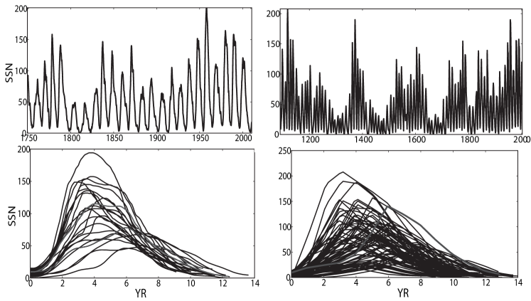
Figure 4: The sunspot data sets. Upper raw: left - SIDC and right - [25](NIMV), lower raw - corresponding cycles distributions

3 Results

The typical time-latitude diagrams for the dynamo models were shown in Figures 2 and 3. The shape of the simulated sunspot cycles in 1D1 model can be seen on the right panel Figure 3. The simulated sunspot cycles for the 2D1 and 2D2 models are shown on the the Figure 5. We can conclude that the shape of the simulated sunspot cycles (and, perhaps, the associated Waldmeier relations) is directly related with the spatial shape of the toroidal magnetic field evaluational patterns. For example, in the 1D1 model the maximum of the butterfly diagram is very close to equator and butterfly wing is elongated toward the pole. In such a pattern of the toroidal magnetic field evolution the decay phase of the sunspot activity is shorter than the rise phase. The opposite situation is in the models 2D1 and 2D2. The physical mechanisms which produce the short rise and the long decay of the toroidal magnetic field activity were discussed recently by Pipin and Kosovichev [29].

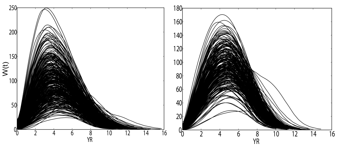
Figure 5: Left panel shows cycles distributions for the model 2D1 and the right panel - model 2D2.

To proceed further we would like to discuss the statistical properties of the cycle parameters those involved in the Waldmeier relations. The 1D models have the much less cycle period than diffusive time of the system. Therefore, we scale the periods of these models by factor $\sim 50$ . The Table 2 show the results for the mean and the variance (standard deviations) for the period, amplitude, rise rate and the shape of the sunspot cycles in the different data sets. From that Table we see that the 1D1 model has the smaller variance in the period, amplitude and rise rate of the cycles as compared to the others data sets. The shape asymmetry of the cycles in 1D1 is opposite to the others cases as well. Also we can see that the mechanism of the helicity loss in the dynamo model influences the mean and variance of the sunspot cycles parameters. In particular, the model 2D2 with the increased diffusive loss of the magnetic helicity has the lower variance of the period and amplitude of the sunspot cycles and has the more symmetric shape of the cycle as compared to the model 2D1. The difference in the synthetic data set of the sunspot cycles provided by NIMV as compared with the SIDC is likely due to the fact that the SIDC data set does not cover the periods with low magnetic activity. This argument is also applied if we compared NIMV and, e.g., 2D1 model. The parameters of the 2D1 model does not allow to have the extended periods of time with very low sunspot cycles.

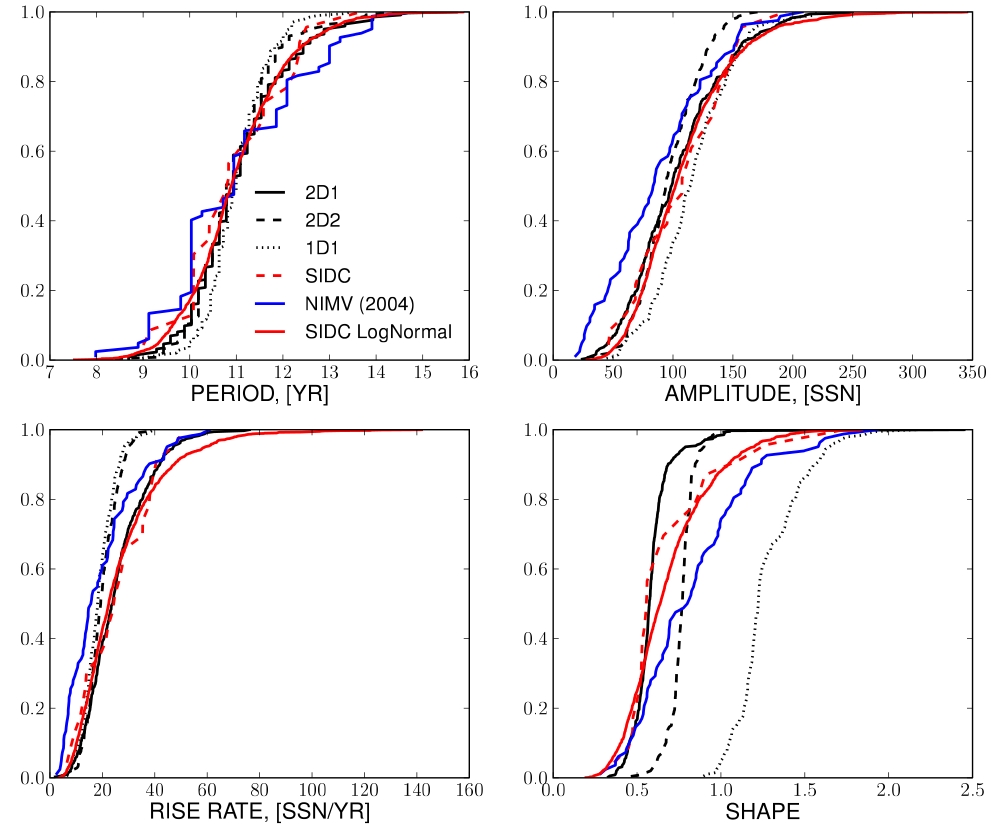
Figure 6: CDF distributions, red line - SIDC the data set, blue line - the data set from [25].

The difference of the the statistical properties of the given data set can be seen in further detail using the cumulative distribution probability functions. The cumulative distributions are constructed as follows. At the beginning, we sort each distribution for each parameter and each model in increasing order. After this we compute the following

$$\mathrm{CDF}(P_{i})=\frac{\sum_{k=1}^{i}k}{N},$$ (9)

where $P_{i}$ is the parameter under consideration (say, the cycle period) having the order number $i$ (after sorting the set in increasing order) and $N$ is the total number of the instances of the given parameter in the set. Equation (9) approximate the probability for the parameter $P$ to have the values in interval between $P_{\rm min}$ and $P_{i}$. The accuracy of the approximation improves under $N\rightarrow\infty$. We will use the log-normal cumulative distribution constructed on the base of the SIDC data set as the reference distribution. The SIDC data set has only 23 instances of the sunspot cycles. To construct the reference log-normal distribution we use the standard mean and variance of the cycles parameters (period, amplitude, rise rate and asymmetry) given in the Table 2. Then take the natural logarithm of them and construct the log-normal distribution of the length 1000 using those mean and variance. The results are shown on the Fig. 6.

It is clearly seen that log-normal distribution is a good fit for the distributions of the sunspot cycles period in the SIDC data set and also for model 2D2. The difference of the SIDC data set from the log-normal distribution is seen in the probabilities distributions for the rise rates and the shape of the cycles. It is, however, unclear if these differences is due to the limited data set of cycles covered by SIDC. The data set produced by the models and the NIMV data set can be equally well approximated by the log-normal distributions (with different mean and variance). For the dynamo models, the difference between the distributions computed by Eq.(9) and the log-normal approximations for them is less visible than for SIDC and NIMV sets.

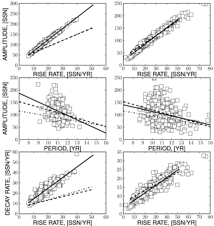
Figure 7: The Waldmeier relations for 1D1 (left) and 2D1 (right) models. The linear fits are shown the solid lines, the dashed lines shows the fits for the SIDC data and the dash-dot line - for the NIMV data.

Fig. 7 shows the Waldmeier relations for the 1D1 and 2D1 models together with their linear fits and also fits for the SIDC and NIMV data sets. The parameters of the linear fits are summarised in the Table 2. It is seen that the model 2D1 is well to reproduce the SIDC data set, and the difference to the NIMV data is not very large. The correspondence of the 2D2 model to the SIDC and the NIMV is not as good as for the 2D1 model. This is also can be expected by results presented in Fig. 6 and by Table 2. Finally, we can conclude that 1D1 model has only qualitative agreement for the relations between the rise rate - amplitude, and the period - amplitude of the sunspot cycles.

4 Discussion and Conclusions

In the paper we have studied the possibility to reproduce the statistical relations of the sunspot activity cycle, like the so-called Waldmeier relations, by means of the mean field dynamo model with the fluctuating $\alpha$-effect. The dynamo model includes the long-term fluctuations of the $\alpha$-effect. The dynamo models employ two types of the nonlinear feedback of the mean-field on the $\alpha$-effect including the algebraic quenching and the dynamic quenching due to the magnetic helicity generation. The paper presents the results for three particular dynamo models.

The presented 1D model is similar to model discussed by Moss et al. [24]. It uses the constant shear and the algebraic quenching of the $\alpha$-effect. The results for this model disagree with observations (SIDC data set) about the shape of the simulated sunspot (decay rate is higher than rise rate) even though it is qualitatively reproduce the basic Waldmeier relations for the Rise Rate-amplitude and the cycle Period-amplitude (see left column in Fig. 7). It was found that the variance of the cycle parameters in the long-term evolution is less than in 2D models. It is interesting, that under the level of noise the 1D models involving the magnetic helicity show the smaller mean even though having the stronger variances of the simulated sunspot parameters. Although we could scale the mean parameters of those models to the observational values, we did not present the results for these models because they have the Waldmeier relations which are quantitatively the same as those presented for 1D1 model in Table 2 and Fig. 7.

We checked the 1D models with the spatially variable shear like that suggested by Kitchatinov et al. [16]. In agreement with the helioseismology results, the given 1D models have the realistic latitudinal profile of the shear (see Eq.(6)). Although, these models qualitatively reproduce the relation between the rise rate and amplitude of the cycle, they fail with the other kind of relations, having the positive correlation between the period and amplitude of the cycle and the equal rate for the rise and decay phase of the simulated sunspot cycles.

Similar to the 1D cases the magnetic helicity contribution to the $\alpha$-effect results to decrease of the toroidal magnetic field strength and to growth the variance of the cycle parameters in the long-term evolution of the magnetic activity. The strong variance of the cycle parameters is expected from SIDC data set and from NIMV as well. For this reason in the paper we discuss the 2D model which involves the effect of the magnetic helicity. The 2D models employ two different description for the magnetic helicity loss, to overcome the problem of the $\alpha$-effect catastrophic quenching. The term $-\overline{\chi}/R_{\chi}\tau_{c}$ in Eq.(3) describes the magnetic helicity loss with the dissipation rate $(\tau_{c}R_{\chi})^{-1}$ without specifying the nature of the loss. Note, that $\tau_{c}$ is varied from about 2 months near bottom of the convection zone to a few hours at the top of the integration domain (which is $0.99R_{\odot}$). Thus, for the $R_{\chi}=200$ used in the model 2D1, the typical decay time for the magnetic helicity is varied from about 4 solar cycles at the bottom of the convection zone to a time which is less than one month at the top of the convection zone. It is not clear if this simple description is satisfactory approximation for the magnetic helicity loss. Therefore we checked the alternative possibility using the diffusive helicity flux. Although, the model that employ the diffusive helicity flux is in satisfactory agreement with SIDC data, the correspondence to observation in this model is not as good as for the model 2D1. We find the the variance of the cycle parameters in the model 2D2 is less than in the model 2D1 while the SIDC and NIMV data sets show higher variances than the model 2D1.

The detailed comparison the results of our models with those given by Karak and Choudhuri [8] is not possible, because we have used a different definition for the amplitude of the cycle and the rise time. They did not give the results for the linear fits coefficients and only provide the correlation coefficients in the Waldmeier relations involving the Rise Rate-amplitude and the Rise Time-Amplitude of the cycle. Bearing in mind the differences in definition that their “high diffusivity model” with fluctuating meridional circulation is comparable with our 2D1 and 2D2 models. It is not clear however what is the typical shape of the cycle in their model. This is an important issue as we have seen in example given by model 1D1. It has qualitative agreement with SIDC data about the period - amplitude and the rise rate - amplitude relations even-though having the rise time of the cycle greater than the decay time.

In the models under consideration, the asymmetry between the ascent and decent phase of the sunspot cycle is inherent from the pattern of the toroidal magnetic field activity. In particular, the 1D1 model has the toroidal magnetic field butterfly diagram with maximum located very close to equator. Therefore, applying the definition Eq.(8) for this type of the toroidal magnetic field evolutional pattern we obtain the decent phase of the sunspot activity shorter than the ascent phase. The opposite situation is in 2D models. There, we relate the sunspot activity with the toroidal field in the subsurface layers. The turbulent diffusivity in the model decrease outward this leads to increases the decay time when the toroidal field gets closer to the surface (see [29]). We find that the effect of the magnetic helicity on the $\alpha$-effect can amplify or saturate the asymmetry of the cycle shape depending on the mechanisms of the helicity loss employed in the model.

It is expected that the nonlinear dynamo mechanisms affect both the magnetic cycle profile and the statistical properties of the cycles. The paper illustrates the impact of the non-linear $\alpha$-effect for the algebraic and the dynamic non-linearities. Recently, Kitchatinov & Olemskoy [17] suggested that the non-linear diffusion could promotes the events similar to the Maunder minimum provided there are the small fluctuations in the $\alpha$-effect. This mechanism does not work in our models, because on the rise phase of the cycle, the growing toroidal magnetic fields results to the turbulent diffusivity quenching and this effect makes the rise phase of the cycle longer, i.e., the smaller turbulent diffusion, the longer evolutionary time scale. The opposite situation is expected for the decay phase of the magnetic cycle.

The comparison of the SIDC data set and the synthetic data set provided by Nagovizyn et al. [25](NIMV) reveals the significant difference in the statistical properties of the cycle parameters. This seems to be a result of the wider cycle variations range covering by the NIMV data set. The model presented in the paper don’t cover the variations seen in NIMV because the selected models almost have no the extended events with low cycles like the so-called Maunder minimum which were observed during the 16-th century. This motivated us to extend our study and explore the models which have the more intermittent variations of the sunspot cycle. This work is planned for the future papers.

Summarizing the main findings of the paper we conclude as follows. We found that the dynamo models, having the reasonably good the time-latitude diagram of the toroidal magnetic field evolution, are able to reproduce qualitatively the inclination and dispersion across the Waldmeier relations with less than 20% Gaussian fluctuations of the $\alpha$-effect. The 2D models have better agreement with observations than 1D. In particular, 1D models fail to reproduce the asymmetric shape of the sunspot cycle with short rise and long decay phases. The statistical distributions of the cycle parameters show the log-normal probability distributions for the all data sets analysed in the paper. The parameters of these distributions are different for all data sets. Again the 1D model is significantly different from others in this sense. The 2D model that employs the simplest form of the helicity loss via the term $-\overline{\chi}/R_{\chi}\tau_{c}$ agrees well with the SIDC, even-though the long-term variations in this model is not intermittent enough, and this seems to be a reason for its difference to the NIMV data set in some aspects. The employ of the diffusive loss in the magnetic helicity evolution equation results to decreasing in the variations of the cycle parameters. The further study of the magnetic helicity transport mechanisms should clarify the likely candidates which are responsible for the magnetic helicity loss from the dynamo region. We have seen that the analysis of the statistical relations of the sunspot cycle may provide the valuable diagnostic tool for this study.

5 Appendix

We describe some parts of the mean-electromotive force. The basic formulation is given in P08. For this paper we reformulate tensor $\alpha_{i,j}^{(H)}$, which represents the hydrodynamical part of the $\alpha$-effect, by using Eq.(23) from P08 in the following form,

$$\alpha_{ij}^{(H)} = \delta_{ij}\left\{3\eta_{T}\left(f_{10}^{(a)}\left(\mathbf{e}\cdot\boldsymbol{\Lambda}^{(\rho)}\right)+f_{11}^{(a)}\left(\mathbf{e}\cdot\boldsymbol{\Lambda}^{(u)}\right)\right)\right\}+$$

$$+ e_{i}e_{j}\left\{3\eta_{T}\left(f_{5}^{(a)}\left(\mathbf{e}\cdot\boldsymbol{\Lambda}^{(\rho)}\right)+f_{4}^{(a)}\left(\mathbf{e}\cdot\boldsymbol{\Lambda}^{(u)}\right)\right)\right\}$$

$$+ 3\eta_{T}\left\{\left(e_{i}\Lambda_{j}^{(\rho)}+e_{j}\Lambda_{i}^{(\rho)}\right)f_{6}^{(a)}+\left(e_{i}\Lambda_{j}^{(u)}+e_{j}\Lambda_{i}^{(u)}\right)f_{8}^{(a)}\right\}.$$

The contribution of magnetic helicity $\overline{\chi}=\overline{\mathbf{a\cdot}\mathbf{b}}$ ($\mathbf{a}$ is a fluctuating vector magnetic field potential) to the $\alpha$-effect is defined as $\alpha_{ij}^{(M)}=C_{ij}^{(\chi)}\overline{\chi}$, where

$$C_{ij}^{(\chi)}=2f_{2}^{(a)}\delta_{ij}\frac{\tau_{c}}{\mu_{0}\overline{\rho}\ell^{2}}-2f_{1}^{(a)}e_{i}e_{j}\frac{\tau_{c}}{\mu_{0}\overline{\rho}\ell^{2}}.$$ (11)

The turbulent pumping, $\gamma_{i,j}$, is also part of the mean electromotive force in Eq.(23)(P08). Here we rewrite it in a more traditional form (cf, e.g., ),

$$\gamma_{ij}=3\eta_{T}\left\{f_{3}^{(a)}\Lambda_{n}^{(\rho)}+f_{1}^{(a)}\left(\mathbf{e}\cdot\boldsymbol{\Lambda}^{(\rho)}\right)e_{n}\right\}\varepsilon_{inj}-3\eta_{T}f_{1}^{(a)}e_{j}\varepsilon_{inm}e_{n}\Lambda_{m}^{(\rho)},$$ (12)

The effect of turbulent diffusivity, which is anisotropic due to the Coriolis force, is given by:

$$\eta_{ijk}=3\eta_{T}\left\{\left(2f_{1}^{(a)}-f_{1}^{(d)}\right)\varepsilon_{ijk}-2f_{1}^{(a)}e_{i}e_{n}\varepsilon_{njk}\right\}.$$ (13)

Functions $f_{\{1-11\}}^{(a,d)}$ depend on the Coriolis number $\Omega^{*}=2\tau_{c}\Omega_{0}$ and the typical convective turnover time in the mixing-length approximation: $\tau_{c}=\ell/u^{\prime}$. They can be found in P08. The turbulent diffusivity is parametrized in the form, $\eta_{T}=C_{\eta}\eta_{T}^{(0)}$, where $\eta_{T}^{(0)}={\displaystyle\frac{u^{\prime}\ell}{3}}$ is the characteristic mixing-length turbulent diffusivity, $u^{\prime}$ is the RMS convective velocity, $\ell$ is the mixing length, $C_{\eta}$ is a constant to control the intensity of turbulent mixing. The others quantities in Eqs.(5,12,13) are: $\mathbf{\boldsymbol{\Lambda}}^{(\rho)}=\boldsymbol{\nabla}\log\overline{\rho}$ is the density stratification scale, $\mathbf{\boldsymbol{\Lambda}}^{(u)}=\boldsymbol{\nabla}\log\left(\eta_{T}^{(0)}\right)$ is the scale of turbulent diffusivity, $\mathbf{e}=\boldsymbol{\Omega}/\left|\Omega\right|$ is a unit vector along the axis of rotation. Equations (5,12,13) take into account the influence of the fluctuating small-scale magnetic fields, which can be present in the background turbulence and stem from the small-scale dynamo (see discussions in). In our paper, the parameter $\varepsilon={\displaystyle\frac{\overline{\mathbf{b}^{2}}}{\mu_{0}\overline{\rho}\overline{\mathbf{u}^{2}}}}$, which measures the ratio between the magnetic and kinetic energies of fluctuations in the background turbulence, is assumed equal to 1. This corresponds to the energy equipartition. The quenching function of the hydrodynamical part of $\alpha$-effect is defined by

$$\psi_{\alpha}=\frac{5}{128\beta^{4}}\left(16\beta^{2}-3-3\left(4\beta^{2}-1\right)\frac{\arctan\left(2\beta\right)}{2\beta}\right).$$ (14)

Note, in notation of P08 $\psi_{\alpha}=-3/4\phi_{6}^{(a)}$, and $\beta={\displaystyle\frac{\left|\overline{B}\right|}{u^{\prime}\sqrt{\mu_{0}\overline{\rho}}}}$.

References

- [1] Artyushkova, M. E., & Sokoloff, D. D. 2006, Magnetohydrodynamics, 42, 3
- [2] Antia, H. M., Basu, S., & Chitre, S. M. 1998, MNRAS, 298, 543
- [3] Brandenburg, A. 2005, ApJ, 625, 539
- [4] Brandenburg, A., & Sokoloff, D. 2002, Geophys. Astrophys. Fluid
- [5] Brandenburg, A., & Subramanian, K. 2004, Astron. Nachr., 325, 400
- [6] Cameron, R., & Schuessler, M. 2008, ApJ, 685, 1291
- [7] Choudhuri, A. R., Schuessler, M., & Dikpati, M. 1995, A& A, 303, L29+
- [8] Karak, B. B., & Choudhuri, A. R., 2011, MNRAS, 410, 1503
- [9] Dikpati, M., & Charbonneau, P. 1999, ApJ, 518, 508
- [10] Dikpati, M., Gilman, P.A., & de Toma, G. 2008, ApJ, 673, L99
- [11] Guerrero, G., Chatterjee, P., & Brandenburg, A. 2010, MNRAS, 409, 1619
- [12] Hathaway, D. H., Wilson, R. M., Reichmann, E. J., 2002, Sol.Phys., 211,357
- [13] Hoyng, P. 1993, A&A, 272, 321
- [14] Kitchatinov, L. L. 2002, A&A, 394, 1135
- [15] Kitiashvili, I. N., & Kosovichev, A. G. 2009, Geophysical and Astrophysical Fluid Dynamics, 103, 53
- [16] Kichatinov, L. L., Ruediger, G., & Kueker, M. 1994, Astron. Astrophys., 292, 125
- [17] Kichatinov, L. L., Olemskoy, S.V, 2010, Geomagnetism and Aeronomy/Geomagnetizm i Aeronomiia, 50, 927
- [18] Kleeorin, N., & Rogachevskii, I. 1999, Phys. Rev.E, 59, 6724
- [19] Krause, F., & Raedler, K.-H. 1980, Mean-Field Magnetohydrodynamics and Dynamo Theory (Berlin: Akademie-Verlag)
- [20] Mitra, D., Candelaresi, S., Chatterjee, P., Tavakol, R., & Brandenburg, A. 2010, Astronomische Nachrichten, 331, 130
- [21] Mitra, D., Moss, D., Tavakol, R., & Brandenburg, A. 2011, A&A, 526, A138+
- [22] Mordvinov, A. V., Kramynin, A. P. 2010, Sol.Phys., 264,269
- [23] Mordvinov, A. V., Kuklin, G. V. 1999, Sol.Phys., 187, 223
- [24] Moss, D., Sokoloff, D., Usoskin, I., & Tutubalin, V. 2008, Solar Phys., 250, 221
- [25] Nagovitsyn, Y. A., Ivanov, V., Miletsky, E., & Volobuev, D. 2004, Solar Physics, 103
- [26] Parker, E. N. 1993, ApJ, 408, 707
- [27] Pipin, V. V. 2008, Geophysical and Astrophysical Fluid Dynamics, 102, 21
- [28] Pipin, V. V., & Kosovichev, A. G. 2011, ApJL, 727, L45
- [29] Pipin, V. V., & Kosovichev, A. G. 2011, ApJ, 741,1
- [30] SIDC. 2010, Monthly Report on the International Sunspot Number, online catalogue, http://www.sidc.be/sunspot-data/
- [31] Soon, W. H., Baliunas, S. L., Zhang, Q., 1994, Sol.Phys., 154, 385
- [32] Stix, M. 2002, The Sun. An Introduction (Springer)
- [33] Subramanian, K., & Brandenburg, A. 2004, Phys. Rev. Lett., 93, 205001
- [34] Usoskin, I. G., Sokoloff, D., & Moss, D. 2009, Solar Phys., 254, 345
- [35] Vitinskij, Yu. I., Kopetskij, M., & Kuklin, G. V. 1986, The statistics of sunspots (Statistika pjatnoobrazovatelnoj dejatelnosti solntsa) (Nauka, Moscow), 298pp
- [36] Waldmeier, M. 1935, Astron. Mitt. Eidgen. Sternwarte Zürich, 14, 105
- [37] Waldmeier, M. 1936, Astron. Nachrichr., 259, 267
- [38] Yoshimura, H. 1975, ApJ, 201, 740
- [39] Zhang, H., Sakurai, T., Pevtsov, A., Gao, Y., Xu, H., Sokoloff, D., & Kuzanyan, K. 2010, MNRAS, 402, L30