Classical Driven Transport in Open Systems with Particle Interactions
and General Couplings to Reservoirs

Abstract

We study nonequilibrium steady states of lattice gases with nearest-neighbor interactions that are driven between two reservoirs. Density profiles in these systems exhibit oscillations close to the reservoirs. We demonstrate that an approach based on time-dependent density functional theory copes with these oscillations and predicts phase diagrams of bulk densities to a good approximation under arbitrary boundary-reservoir couplings. The minimum or maximum current principles can be applied only for specific bulk-adapted couplings. We show that they generally fail to give the correct topology of phase diagrams but can still be useful for getting insight into the mutual arrangement of different phases.

Lattice gases provide useful models for investigating driven particle transport in biological, chemical and physical systems Hille (2001); Nitzan (2006). They are used to study Brownian ratchets and motors Hänggi and Marchesoni (2009); Einax et al. (2010), organic photovoltaic cells Einax et al. , and traffic on networks Neri et al. (2011), to name only some recent applications. In these examples, the asymmetric simple exclusion process (ASEP) appears as a basic building block for the description of low-dimensional transport. As such it has developed into one of the standard models for investigating nonequilibrium steady states (NESS). In the ASEP, particles hop under the influence of a bias field and cannot occupy the same place. For open boundary conditions, these biased systems show intriguing phenomena, like boundary-induced phase transitions Krug (1991), emergence of shock fronts Kolomeisky et al. (1998), and self-organized pattern formation Boal and Zia (1991). To explain these phenomena, it is generally sufficient to consider the totally asymmetric simple exclusion processes (TASEPs), where the particle transport in the bias direction is unidirectional.

Much progress has been made in the past to understand ASEPs and TASEPs (for reviews, see Refs. Derrida (1998); Golinelli and Mallick (2006); Blythe and Evans (2007)), but only a few studies so far have addressed TASEPs with particle-particle interaction going beyond hard-core repulsions Katz et al. (1984); Krug (1991); Popkov and Schütz (1999); Antal and Schütz (2000); Hager et al. (2001); Dierl et al. (2011). While in this case a complete description of the NESS seems to be out of reach for open systems, it has been shown that the minimum/maximum current principles Krug (1991); Popkov and Schütz (1999), or the domain-wall (shock-front) theory Kolomeisky et al. (1998); Popkov and Schütz (1999); Bauer and Bernard (1999), can be used in a specific model setup to predict phase diagrams of the bulk density. This setup requires that the relations between correlation functions and densities close to the system-reservoir boundaries are the same as in the bulk. To ensure this, a particular way of particle injection and ejection has to be taken, which was used in Refs. Popkov and Schütz (1999); Antal and Schütz (2000); Hager et al. (2001); Dierl et al. (2011).

However, realistic reservoirs are not of that type but are specified by only a few control parameters, as, for example, temperature and chemical potential. It is therefore needed to develop methods that can deal with such situations both on basic reasons and in view of various applications. For example, in driven transport through molecular bridges (e.g., in the incoherent limit for weak coupling to leads) Nitzan (2001); Harbola et al. (2006), one does not specify a complicated bath-system coupling, but is led by the fact that the typical relaxation dynamics in the bath is much faster than in the system. Accordingly, the baths are supposed to be in equilibrium and characterized essentially by their chemical potential.

In this Letter we consider a TASEP with nearest-neighbor interactions as sketched in Fig. 1 and show that the couplings of the system to the reservoirs have a strong influence on the density profiles in the nonequilibrium steady state (NESS). In general, oscillations of these profiles occur close to the boundaries, similar as they are known for equilibrium systems. We present a theory that is able to cope with these oscillations and to describe the density profiles to a good approximation. Based on the theory, the phase diagram of the bulk density can be determined. Our theoretical approach provides a general method to predict such phase diagrams for driven systems with interactions under general boundary-reservoir couplings.

To demonstrate our theoretical approach we consider as an example the following specific model, see Fig. 1: Particles with repulsive nearest-neighbor interaction of strength $V>0$ perform a unidirectional hopping motion between neighboring sites of a lattice with $N$ sites and are thereby transported from a left to a right particle reservoir. The microstate of the system is specified by the set of occupation numbers $\boldsymbol{n}=\{n_{i}\}$, $i=1,\ldots,N$, where $n_{i}=0$ or $1$ if the corresponding site is vacant or occupied by a particle. The jump rate of a particle from a site $i$ to a vacant neighboring site $(i+1)$ is $\Gamma_{i}=\exp(-\Delta E/2)$, where $\Delta E$ is the energy difference (in units of the thermal energy) between the final and initial state after and before the jump.

When $V>V_{\rm c}=2.89$, the bulk current-density relation of this model exhibits a double-hump structure with two maxima at densities $\rho_{{\rm max},1}$ and $\rho_{{\rm max},2}$, and a minimum in between at $\rho=0.5$ Dierl et al. (2011). The bulk dynamics are considered to apply to jumps from sites $i=2,\ldots,(N-2)$, while couplings to the reservoirs are taken into account for injections from and ejections to the reservoirs. In addition we need to specify rates for jumps from sites $i=1$ and $(N-1)$, where, if one adopted the bulk rates, a nearest- and a next-nearest-neighbor site would be missing to the left and right, respectively. As sketched in Fig. 1, two cases of boundary couplings are considered. These couplings are referred to as “bulk-adapted” and “equilibrated-bath” coupling and explained for the left reservoir in the following. Corresponding couplings are applied to the right reservoir.

For the equilibrated-bath coupling [Fig. 1(b)], the left reservoir is considered to be an equilibrated ideal Fermi gas with a chemical potential $\mu_{\rm\scriptscriptstyle L}$, corresponding to a reservoir density $\rho_{\rm\scriptscriptstyle L}=1/[\exp(-\mu_{\rm\scriptscriptstyle L})+1]$. Accordingly, we write for the rate $\Gamma_{\rm\scriptscriptstyle L}$ of particle injection $\Gamma_{\rm\scriptscriptstyle L}(n_{2})=\rho_{\rm\scriptscriptstyle L}\exp[(\mu_{\rm\scriptscriptstyle L}-n_{2}V)/2]$, and $\Gamma_{1}(n_{3})=\exp(-n_{3}V/2)$ for the jump rate from site one.

The bulk-adapted coupling [Fig. 1(a)] is arranged in such a way that the system can be viewed as being continued into a reservoir with density $\rho_{\rm\scriptscriptstyle L}$, corresponding to relations between correlation functions  $\langle n_{i}n_{j}\ldots\rangle$, and densities $\rho_{i}=\langle n_{i}\rangle$ as in the bulk, where $\langle\ldots\rangle$ denotes an average over the distribution of microstates in the NESS. In a closed bulk (ring) system, when an initial configuration $\{n_{i+1}=0,n_{i+2}\}$ would be given, two rates are possible for a particle jump from site $i$ (i.e. $n_{i}=1$): $\Gamma_{i}=\exp(-n_{i+2}V/2)$, if $n_{i-1}=0$, while $\Gamma_{i}=\exp[(1-n_{i+2})V/2]$, if $n_{i-1}=1$. For given $\{n_{i+1}=0,n_{i+2}\}$, let us denote by $p(01|0n_{i+2})$ and $p(11|0n_{i+2})$ the conditional probabilities for the configurations $\{n_{i-1},n_{i}\}=\{0,1\}$ and $\{n_{i-1},n_{i}\}=\{1,1\}$ to occur in the NESS of a closed bulk system with density $\rho_{\rm\scriptscriptstyle L}$ and interaction $V$, respectively. The injection rate $\Gamma_{\rm\scriptscriptstyle L}(n_{2})$ then results from a weighting of rates with the probabilities $p(01|0n_{2})$ and $p(11|0n_{2})$ corresponding to virtual configurations $\{n_{-1}=0,n_{0}=1,n_{1}=0,n_{2}\}$ and $\{n_{-1}=1,n_{0}=1,n_{1}=0,n_{2}\}$ at the boundaries, i.e., $\Gamma_{\rm\scriptscriptstyle L}(n_{2})=p(01|0n_{2})\exp(-n_{2}V/2)+p(11|0n_{2})\exp[(1-n_{2})V/2]$. Analogously, $\Gamma_{1}(n_{3})=p(0|10n_{3})\exp(-n_{3}V/2)+p(1|10n_{3})\exp[(1-n_{3})V/2]$. For a practical implementation of a corresponding kinetic Monte Carlo (KMC) simulation, the conditional probabilities $p(.|.)$ are determined from separate KMC simulations of periodic ring systems with a particle density $\rho=\rho_{\rm\scriptscriptstyle L}$ as indicated in Fig. 1(a). The rates for the two models are summarized in sup .

KMC simulations have been carried out for both the bulk-adapted and the equilibrated-bath coupling and results are shown by the squares and circles in Fig. 2 for $V=2V_{\rm c}$, $\rho_{\rm\scriptscriptstyle L}=0.9$ and $\rho_{\rm\scriptscriptstyle R}=0.7$. As a consequence of the specific arrangements in the bulk-adapted case, monotonously varying density profiles are obtained, similar as in the TASEP with hard-core repulsion only. The value of the bulk density $\rho_{\rm\scriptscriptstyle B}\cong 0.70$ agrees with that predicted from applying the maximum current principle to the bulk current-density relation. For the equilibrated-bath coupling by contrast, pronounced oscillations appear at the boundaries. This implies that methods relying on the bulk current-density relation (minimum/maximum current principles, shock-front/domain-wall theories) cannot be applied any more to predict the bulk densities. In fact, Fig. 2 shows that a value $\rho_{\rm\scriptscriptstyle B}\cong 0.40$ is obtained for the equilibrated-bath coupling, which differs from that for the bulk-adapted coupling.

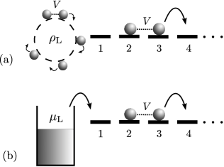
Figure 1: Sketch of the model and illustration of the particle injection for (a) the bulk-adapted, and (b) the equilibrated-bath couplings. Right reservoirs are not shown.

The question is whether a theory can successfully account for the bulk densities and associated phase diagrams for interacting driven particle systems that generally will show density oscillations at the boundaries. Mean-field theories with simple factorization schemes, as, for example, $\langle n_{i}n_{j}\rangle\simeq\langle n_{i}\rangle\langle n_{j}\rangle$ fail for the model introduced here, since they are not even capable to predict the double-hump structure in the bulk current-density relation. We now show that the application of the time-dependent density functional theory (TDFT) presented in Heinrichs et al. (2004); Dierl et al. (2011) can deal with the complications associated with the density oscillations. In this approach the average current $j_{i}$ from site $i$ to site $(i+1)$ in the bulk ($i=2,\ldots,(N-2)$) is given by

$$j_{i} =\left[(\rho_{i+2}-C_{i+1})e^{-V/2}+\tilde{\rho}_{i+1}-\rho_{i+2}+C_{i+1}\right]$$

$$\hskip 13.00005pt{}\times\frac{\rho_{i}-C_{i}}{\rho_{i}\tilde{\rho}_{i+1}}\left[\rho_{i}-C_{i-1}+e^{V/2}C_{i-1}\right]\,,$$ (1)

where $\rho_{i}=\langle n_{i}\rangle$ and $\tilde{\rho}_{i}=1-\langle n_{i}\rangle=1-\rho_{i}$ are the particle and hole density, respectively, and $C_{i}=\langle n_{i}n_{i+1}\rangle$ is the two-point correlation function Buschle et al. (2000),

$$C_{i}=\exp\left(-V\right)\frac{\left(\rho_{i}-C_{i}\right)\left(\rho_{i+1}-C_{i}\right)}{1-\rho_{i}-\rho_{i+1}+C_{i}}\,.$$ (2)

This expression can be explicitly solved to yield functions $C_{i}=C_{i}(\rho_{i},\rho_{i+1})$ and in this way, the bulk currents $j_{i}$ in Eq. (Classical Driven Transport in Open Systems with Particle Interactions and General Couplings to Reservoirs) become functionals of the density profile $\boldsymbol{\rho}(t)=\{\rho_{i}(t)\}$.

For the bulk-adapted couplings, Eq. (Classical Driven Transport in Open Systems with Particle Interactions and General Couplings to Reservoirs) applies also at the boundaries, that means for $i=0$, 1, $(N-1)$ and $N$ com . For the equilibrated-bath couplings, however, different functional structures are obtained:

$$j_{0} =\rho_{\rm L}e^{\mu_{\rm L}/2}\left[\left(\rho_{2}-C_{1}\right)e^{-V/2}+\tilde{\rho}_{1}-\rho_{2}+C_{1}\right]\,,$$ (3a)

$$j_{1} =\frac{\rho_{1}-C_{1}}{\tilde{\rho}_{2}}\left[\left(\rho_{3}-C_{2}\right)e^{-V/2}+\tilde{\rho}_{2}-\rho_{3}+C_{2}\right]\,,$$ (3b)

$$j_{N-1} =\frac{\rho_{N-1}-C_{N-1}}{\rho_{N-1}}\left[C_{N-2}e^{V/2}+\rho_{N-1}-C_{N-2}\right]\,,$$ (3c)

$$j_{N} =\tilde{\rho}_{\rm R}e^{-\mu_{\rm R}/2}\left[C_{N-1}e^{V/2}+\rho_{N}-C_{N-1}\right]\,.$$ (3d)

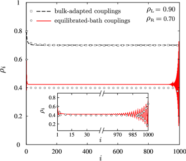
Figure 2: (Color online) Steady-state density profiles for $V=2V_{\rm c}$ from KMC simulations (symbols) in comparison with the TDFT predictions (lines). For the KMC results averages were performed over $10^{9}$ particle jumps in the steady state. The inset shows the density profile for the equilibrated-bath couplings close to the left and right boundary, respectively.

To compare the predictions of this theory with the KMC results we have integrated numerically the coupled set of rate equations ${\rm d}\rho_{i}(t)/{\rm d}t=j_{i-1}(t)-j_{i}(t)$ ($i=1,\,\ldots,N$) with the currents given by (Classical Driven Transport in Open Systems with Particle Interactions and General Couplings to Reservoirs)-(3) and evaluated the long-time limit to analyze the NESS. As shown in Fig. 2, the density profile from the TDFT for the bulk-adapted coupling agrees well with KMC results. Surprisingly, also the oscillations of the KMC density profiles for the equilibrated-bath couplings are closely reproduced by the TDFT, see the inset of Fig. 2. Moreover, the TDFT gives a value $\rho_{\rm\scriptscriptstyle B}\cong 0.42$ that is only slightly larger than the corresponding KMC value $\rho_{\rm\scriptscriptstyle B}\cong 0.40$. For the steady-state currents we find $j_{\rm\scriptscriptstyle NESS}=0.174$ in the KMC and $j_{\rm\scriptscriptstyle NESS}=0.149$ in the TDFT.

With the density profiles determined from either KMC or TDFT we can identify the singularities in the dependence of the bulk density on the reservoir densities $\rho_{\rm\scriptscriptstyle L}$ and $\rho_{\rm\scriptscriptstyle R}$. Corresponding transition lines are shown in the phase diagram of Fig. 3 for $V=2V_{\rm c}$, and for (a) the bulk-adapted and (b) the equilibrated-bath couplings. Overall, the TDFT accounts well for the phase transitions as determined from the KMC simulations. Due to the construction of the bulk-adapted couplings, the knowledge of the exact bulk current-density relation in the NESS would allow one to determine exactly the phase diagram by applying the minimum/maximum current principles. In this way seven phases are identified in Fig. 3(a). Since the TDFT does not yield the bulk current-density relation in the NESS exactly, small deviations are seen in Fig. 3(a) between KMC and TDFT results.

The strongly different diagram in Fig. 3(b) shows that the minimum/maximum current principles are no longer successful. By contrast, the TDFT accounts well for the five phases identified in the KMC simulations. There are three phases, where $\rho_{\rm\scriptscriptstyle B}$ is some function of either $\rho_{\rm\scriptscriptstyle L}$ or $\rho_{\rm\scriptscriptstyle R}$, and a maximum current phase with $\rho_{\rm\scriptscriptstyle B}=\rho_{{\rm max},1}$ and a minimum current phase with $\rho_{\rm\scriptscriptstyle B}=0.5$. Generally, $\rho_{\rm\scriptscriptstyle B}$ must be either determined by $\rho_{\rm\scriptscriptstyle L}$ or $\rho_{\rm\scriptscriptstyle R}$, or by the extrema in the bulk current-density relation, since the minimum/maximum current principles still apply in the inner bulk regions, where the density profiles are monotonously varying. The absence of a maximum current phase with $\rho_{\rm\scriptscriptstyle B}=\rho_{{\rm max},2}$ for the equilibrated-bath couplings means that also the topology of the phase diagram in Fig. 3(b) is changed compared to that in Fig. 3(a). It can be shown that this change of topology is generally possible and that there are no further hidden phases in addition to the ones shown in Fig. 3(b) Die . Those phases, which appear in Fig. 3(b), have a connection to the ones in Fig. 3(a) in the sense that their mutual arrangement remains the same.

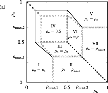
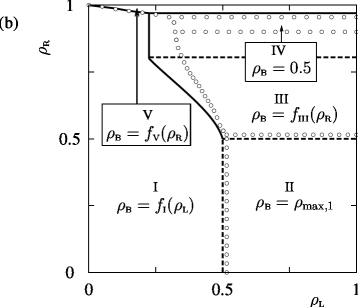
Figure 3: Phase diagrams of the NESS for (a) the bulk-adapted and (b) the equilibrated-bath couplings at $V=2V_{\rm c}$. KMC results for the phase transitions are marked by the symbols and TDFT results by the lines (solid lines for first-order and dashed lines for second-order phase transitions). In (a) seven phases are obtained, where the bulk density $\rho_{\rm\scriptscriptstyle B}$ equals either the reservoir densities $\rho_{\rm\scriptscriptstyle L}$ or $\rho_{\rm\scriptscriptstyle R}$, or the value $0.5$ in the minimum current phase, or the two possible values $\rho_{{\rm max},1}$ or $\rho_{{\rm max},2}$ in the maximum current phases. In (b) a maximum current phase with $\rho_{\rm\scriptscriptstyle B}=\rho_{{\rm max},1}$, a minimum current phase with $\rho_{\rm\scriptscriptstyle B}=0.5$, and three phases with reservoir-controlled densities $\rho_{\rm\scriptscriptstyle B}=f_{\rm\scriptscriptstyle I}(\rho_{\rm\scriptscriptstyle L})$, $\rho_{\rm\scriptscriptstyle B}=f_{\rm\scriptscriptstyle III}(\rho_{\rm\scriptscriptstyle R})$, and $\rho_{\rm\scriptscriptstyle B}=f_{\rm\scriptscriptstyle V}(\rho_{\rm\scriptscriptstyle R})$ are obtained, where the different functions of $\rho_{\rm\scriptscriptstyle L}$ or $\rho_{\rm\scriptscriptstyle R}$ are determined from the simulated or calculated density profiles. The labeling by roman numbers in (a) and (b) has been chosen in such a manner that corresponding phases have equal numbers.

In conclusion we have shown that the theoretical approach based on the TDFT can cope with the problem of driven lattice gases with extended interactions, where oscillations in densities and correlation functions naturally occur at the boundaries. The oscillations imply that the minimum/maximum current principles are no longer sufficient, since they can only be applied in an inner bulk region, where the density profile varies monotonously. When, for unmodified bulk dynamics, deliberately changing the boundary couplings to the bulk-adapted ones in order to enable the use of the minimum/maximum current principles, the currents and bulk densities in the NESS as well as the associated phase diagrams are strongly influenced. The principles are nevertheless useful to justify the identification of possible phases on the basis of a known bulk current-density relation. The investigation of the bulk-adapted couplings can be helpful to predict the mutual arrangement of those phases that appear for the boundary couplings of interest.

We believe that our theory can be useful to explore a wider range of driven open systems which are of importance for many biological processes and electronic transport phenomena in small molecular devices that can be treated within the incoherent classical limit.