Effective and exact holographies
from symmetries and dualities

Abstract

The theoretical basis of the phenomenon of effective and exact dimensional reduction, or holographic correspondence, is investigated in a wide variety of physical systems. We first derive general inequalities linking quantum systems of different spatial (or spatio-temporal) dimensionality, thus establishing bounds on arbitrary correlation functions. These bounds enforce an effective dimensional reduction and become most potent in the presence of certain symmetries. Exact dimensional reduction can stem from a duality that (i) follows from properties of the local density of states, and/or (ii) from properties of Hamiltonian-dependent algebras of interactions. Dualities of the first type (i) are illustrated with large-$n$ vector theories whose local density of states may remain invariant under transformations that change the dimension. We argue that a broad class of examples of dimensional reduction may be understood in terms of the functional dependence of observables on the local density of states. Dualities of the second type (ii) are obtained via bond algebras, a recently developed algebraic tool. We apply this technique to systems displaying topological quantum order, and also discuss the implications of dimensional reduction for the storage of quantum information.

1 Introduction

Spatial (or space-time) dimensionality, topology, and symmetry are central concepts in physics. This article studies a phenomenon, that of dimensional reduction or holographic correspondences, that highlights how these concepts may come together to produce particularly striking signatures.

The dimension of a system is one of its most basic characteristics and typically represents an important measure of its complexity. Dimensional reduction and holographic correspondences refer to the fact that the “apparent”, or “obvious” dimension $D$ of a system may not be the dimension $d$, $d<D$, that best characterizes its response to experimental probes and its information content. We speak of dimensional reduction when the observable physical properties of a system in $D$ dimensions behave as if it were $d$-dimensional. We argue for a holographic correspondence when two systems of different dimensionality seem capable of storing and processing comparable amounts of information. Both notions, often undistinguished in current literature, appear in numerous fields including condensed matter, cold atom, high-energy, and black-hole physics. Given the cross-disciplinary nature of the subject there is a need to better understand the physical and mathematical basis of dimensional reduction and holographic correspondences. We believe that this understanding should be rooted in basic principles than in properties of specific models.

This article constitutes an attempt to study exact and effective dimensional reductions, and holographic correspondences within a unified framework. Our approach relies on the recent theory of dualities [1], and a new theorem that constrains arbitrary correlators of a quantum theory in $D$ dimensions. The obtained inequalities and bounds afford a practical notion of effective dimensional reduction because they are specified by homologous correlators of an associated, local, $d<D$ dimensional theory. Also they become specially useful in the presence of ${\bf d}$-dimensional gauge-like symmetries (or $\bf d$-GLSs for short) [2, 3], with ${\bf d}<D$, a geometrically distinguished set of symmetries that we will discuss further below. The notion of exact dimensional reduction is further linked to the existence of a duality, mapping the $D$-dimensional theory to a $d$-dimensional one. In such situations inequalities may be replaced by exact equalities. We also introduce the concept of dimensional reduction by the density of states, a concept that may find its way to practical applications in the form of either exact or effective versions, depending on the problem. We illustrate this technique with $O(n)$ type vector theories. Finally, we will show that exact dimensional reduction is sometimes connected to a holographic-like entropy that scales as the surface of the system, and use large-$n$ vector theories to illustrate this point. Remarkably, our take on dimensional reduction/holographic correspondences will allow us to discuss limitations on the storage and robustness of quantum information.

While dimensional reduction/holographic correspondences may seem to be exotic phenomena, they can in fact appear in many systems as the natural consequence of a wealth of physical mechanisms:

(1) Restrictions from conservation laws. In some cases, a conservation law (that can be formalized as a gauge constraint) favors sliding dynamics along preferred directions while forbidding motion along other directions. For example, the glide principle [4] for elastic solids dictates that dislocations move preferentially along directions that are determined by their topological charges or Burger’s vectors.

(2) Reduced kinetics and interactions along one or more directions. In many condensed matter systems a dimensional reduction can occur due to the confinement of electrons/atoms along planes or lines (e.g., wires), whereby certain directions become irrelevant. Reduced tunneling, for instance, can appear along certain directions, as in the case of high-$T_{c}$ cuprates and some other layered systems, due to relatively large separation between planes that suppresses interplane couplings and tunneling from one layer to the next. Similar decoupling can occur in magnetic systems with spin exchange interactions on geometrically frustrated lattices [5], where the coupling between planes (or other lower-dimensional subvolumes) along one or more directions becomes negligible. In all of these systems, the effective physical interactions and/or kinetic hopping matrix elements describe a lower-dimensional system. Many of these systems are locally inhomogeneous with electrons constrained in some way, but at large distances the symmetry between different directions is restored. That is, in such cases, converse to the Kaluza-Klein type compactifications that we list next, dimensional reduction may (but need not) emerge at local scales. At short distance scales the system is effectively of a lower dimensionality than it is at large distance scales.

(3) Kaluza-Klein compactification. Dimensional reduction can be achieved geometrically by compactifying $(D-d)$ spatial dimensions of a theory through the Kaluza-Klein [6] procedure. At low energies or temperatures, excitations along these “small dimensions” are suppressed, leading to an effective $d$-dimensional theory. That is, dimensional reduction emerges at low energies and large distances. This type of dimensional reduction is important in string [7] and supergravity theories, and it has been suggested recently [8, 9] that may also help to address the Langlands duality which is an open problem in basic mathematics.

(4) Gravity-gauge dualities (AdS-CFT). A seemingly different, more subtle, and very powerful form of dimensional reduction is offered by the AdS-CFT (or more general gravity-gauge) holographic correspondences (dualities). This correspondence relates, via a putative strong-weak coupling duality, different theories: string theory as a theory of quantum gravity on an Anti de Sitter (AdS) background in $D$ dimensions, and a conformal field theory (CFT) in $d=D-1$ space-time dimensions. Since its initial discovery [10], the AdS-CFT correspondence [10, 11, 12, 13, 14] has been a source of inspiration for many ideas and applications. Apart from its original use in string theory, as a gravity-gauge correspondence [10], it has led to many other applications that include hadronic hydrodynamics [15] and fundamental questions relating to transport in strongly correlated systems [16]. Similar forms of an AdS-CFT type correspondence were conjectured for cold atom systems with Schrödinger type dynamics [17].

This incomplete list of known mechanisms underscores the multitude of disparate phenomena that may lead to dimensional reduction and holographic-like correspondences. This article will describe simple tools that can help address this diversity in a coherent way. As mentioned already, we distinguish between two scenarios:

(i) Effective dimensional reduction. This possibility has, for the most part, not been explored before (especially in quantum theories), and forms a cornerstone of this article. Items (1), (2), and (3) above can be seen as realizations of this type of dimensional reduction. We will illustrate how inequalities with bounds on arbitrary correlation functions, typically strengthened by the presence of $\bf d$-GLSs, relate to an effective dimensional reduction.

(ii) Exact dimensional reduction. We identify this scenario with the existence of dualities connecting theories of different dimensionality. These dualities may be exact or asymptotically so in some limit (such as the large-$n$ limit or the weak coupling limit). Case (4) is often conjectured to be exact yet still largely remains to be proved. The AdS-CFT correspondence has, however, been convincingly established in the large-$n$ limit and several related $SU(n)$ matrix and other models.

In general, an effective dimensional reduction is very different in nature from an exact dimensional reduction, whence the spectrum of a $D$-dimensional system attains a form akin to that of a theory in ${d}<D$ dimensions with local interactions. In this paper, this effective scenario is characterized in terms of a flexible formalism that can describe a range of situations that go from “very weak” to “very strong” dimensional reduction. It is essential then to recognize ingredients that will favor the strongest forms of effective dimensional reduction. Symmetries, and more specifically, the ${\bf d}$-GLSs that we describe in the next section, are one such ingredient. In such cases, those symmetries mandate how the bounding $\bf d$-dimensional correlation functions decay with distance.

The concept of exact dimensional reduction (ii) is more restrictive, and its connection to ${\bf d}$-GLS is less clearly understood. If an exact equivalence is present between all possible correlation functions in two different theories then it will be natural to conjecture that a duality (i.e., an exact unitary mapping [1]) connects the theory that displays lower- ($d$) dimensional behavior, yet described as high- ($D$) dimensional theory, to a dual theory explicitly $d$-dimensional. Then the inequalities saturate and become equalities. This occurs, for instance, in some special models [2, 18], such as Kitaev’s model [19], that may be constructed and solved using these unitary mappings. As we will show, this occurs far more generally in the large-$n$ limit of rather general $O(n)$ type vector theories. The crux of this result is that in systems such as large-$n$ vector theories, the partition function (or generating functional) of the system can be expressed in terms of an effective density of states functional. Transformations between systems that reside in different (space/space-time) dimensions that preserve this density of states, while maintaining the locality of the theory, automatically correspond to (dimension reducing) duality transformations.

We expect, though, that the most complex cases of dimensional reduction/holographic correspondences may be understood as the combined use of (i) and (ii).

2 Systems of study

The results reported in this work hold for a very broad class of systems. Throughout, we will consider arbitrary quantum systems (or their classical descendants) in $D$- spatial (or space-time) dimensions with Hilbert spaces which are either finite or denumerably infinite. The theories to be directly analyzed are defined on a $D$-dimensional lattice of volume $\Lambda$. When alluded to, continuum field theories will be understood to be represented by the continuum (vanishing lattice size $a$) limit of an appropriately defined lattice field theory regularizing it. The Hamiltonians (or Euclidean actions) of the systems that we address have interactions local in space (or space-time), i.e., have couplings that veer to zero at large spatial (or temporal) separations. In the thermodynamic ($\Lambda\rightarrow\infty$) limit we will, at times, replace pertinent sums over the Fourier modes ${\bf k}$ associated with lattice systems by corresponding integrations over the first Brillouin zone. For instance, in the case of a square lattice system, $k_{\mu}=2\pi l_{\mu}/L$ with $L$ the linear lattice size along the $\bm{e}_{\mu}$ direction, $\mu=1,2$, $-L/2a<l_{\mu}\leq L/2a$ being integers, with $a$ the lattice constant. The first Brillouin zone is spanned by $-\pi/a<k_{\mu}\leq\pi/a$.

Symmetries represent an important element of our analysis. The most general symmetry ${\cal U}$ of a system with a Hamiltonian $H$ can be described as a direct sum of arbitrary unitary transformations $U(N_{E_{i}})$ that act non-trivially only on their corresponding subspaces of fixed energy $E_{i}$ and of dimension $N_{E_{i}}$. That is, the direct sum of unitary transformations

$${\cal U}=\sum_{{i}}\ U(N_{E_{i}})$$ (1)

constitutes a symmetry of the system, i.e., ${\cal U}^{\dagger}H{\cal U}=H$, for arbitrary $U(N_{E_{i}})$. Conversely, if ${\cal U}$ is a symmetry and $H=\sum_{{i}}E_{i}P_{i}$ is the spectral decomposition of $H$, then ${\cal U}$ has the structure of Eq. (1) above, with $U(N_{E_{i}})={\cal U}P_{i}$. Typically, unitary operations of the type of Eq. (1) may correspond to non-local operations. In contrast, the symmetries that are most relevant to dimensional reduction have well defined spatial support.

This observation (that will be illustrated often in this paper) leads to the notion of ${\bf d}$-GLSs. As alluded to earlier, these are symmetry operations (of codimension $D-{\bf d}$) that act non-trivially only within a ${\bf d}$-dimensional physical space. Technically, a symmetry is termed ${\bf d}$-GLS if fields acted on by the symmetry operators ${\cal U}_{\bf d}$ are affected within a region of $\bf d$-dimensional support [2, 3]. For instance, local (gauge) symmetries are of dimension ${\bf d}=0$. Similarly, global symmetry operators act on all of the fields of the system and thus their dimension is ${\bf d}=D$ (that of the entire system). In between these two extremes of local (${\bf d}=0$) and global (${\bf d}=D$) symmetries there is an intermediate regime where the symmetry operators act on a $0<{\bf d}<D$ dimensional spatial region. It was recently shown [2] that ${\bf d}$-GLSs can mandate the appearance of topological quantum order (TQO) [20]. In continuum space-time ${\bf d}$-GLSs may asymptotically include, as a particular case, the conformal symmetries that appear in conformal fields theories (CFTs) but are not limited to these.

It will be useful in the following to keep in mind specific simple examples for which our theorems have easy to grasp yet non-trivial consequences. The spin $S=1/2$, $D=2$ compass model [2, 3] on a square lattice is one of many such examples. It is often specified by the Hamiltonian

$$H_{\sf compass}=-\sum_{{\bm{x}}\in\Lambda}(J_{1}\ \sigma^{x}_{{\bm{x}}}\sigma^{x}_{{\bm{x}}+{\bm{e_{1}}}}+J_{2}\ \sigma^{y}_{{\bm{x}}}\sigma^{y}_{{\bm{x}}+{\bm{e_{2}}}}),$$ (2)

with exchange couplings $J_{\mu}$, where $\sigma_{{\bm{x}}}^{\alpha=x,y}$ are Pauli operators located at the lattice site ${\bm{x}}=i^{1}\bm{e}_{1}+i^{2}\bm{e}_{2}$ (${\bm{x}}\in\Lambda$). Its ${\bf d}=1$-GLSs

$$X_{i^{1}}=\prod_{i^{2}}\sigma^{x}_{i^{1},i^{2}},\ \ \ \ Y_{i^{2}}=\prod_{i^{1}}\sigma^{y}_{i^{1},i^{2}},$$ (3)

($[H_{\sf compass},X_{i^{1}}]=0=[H_{\sf compass},Y_{i^{2}}]$) satisfy the algebra

$$\ \{X_{i^{1}},Y_{i^{2}}\}=0,\ \ \ \ [X_{i^{1}},X_{{i^{1}}^{\prime}}]=[Y_{i^{2}},Y_{{i^{2}}^{\prime}}]=0.$$ (4)

The Xu-Moore model [21], studied before in connection to dimensional reduction, is dual to the compass model [1, 22].

3 Effective dimensional reduction via bounds

As explained in the introduction, our approach to effective dimensional reduction is based on inequalities. These inequalities are the subject of a theorem on an effective quantum dimensional reduction (EQDR) that we prove in this section.

Intuitively speaking, a system is intrinsically $D$-dimensional if it cannot be simulated by a lower-dimensional one (a higher-dimensional simulator is always possible provided some redundancy is allowed [23]). This idea provides the basis for a good definition of intrinsically $D$-dimensional, but fails to provide simple, practical criteria to search for dimensional reduction. The EQDR theorem provides one such criterion. The idea is that $D$-dimensional systems have observables $f$ that specifically probe $d$-dimensional sub-volumes $\Gamma$, $d\leq D$, of the $D$-dimensional space $\Lambda$. The EQDR theorem illustrates that under certain (not very stringent) conditions, the expectation values of these $d$-dimensional observables are both bounded from above and from below by expectation values taken within effective $d$-dimensional theories. Thus, we can use the behavior of these bounds (e.g., how stringent they are for specific theories) as indicators to search for effective dimensional reduction. As stressed in the introduction, the EQDR theorem becomes most useful in the presence of suitable d-GLSs.

The EQDR theorem exploits features of quantum mechanics that force us to reconsider the notion of localizability. This notion poses a problem that was perhaps first fully appreciated in the context of entanglement [24, 25, 26] but was also carefully considered in connection to the notion of particle (more specifically, the position of a particle) in quantum field theory [27]. Remarkably, the notions of localizability that emerged from those two lines of inquiry are (as far as we can see) conceptually different, and exploit different mathematical structures on the space of states. Hence, in order to apply the EQDR theorem to quantum field theories and many-body systems we need to introduce a redundant representation of the state space of identical particles, and keep the constraint of indistinguishability explicit in the form of a projector onto subspaces of completely (anti)symmetric state vectors. This enables us to treat fermions and bosons. In the current work, we do not discuss the extension of the EQDR theorem to systems with anyon statistics.

3.1 A theorem on effective quantum dimensional reduction (EQDR theorem)

The EQDR theorem is inspired by an analogous theorem for classical statistical mechanics [3]. Hence it is convenient to review briefly this theorem on classical dimensional reduction to motivate its quantum analogues and to introduce some useful notation.

Consider a classical model of statistical mechanics that, for concreteness, has its degrees of freedom defined on the sites of a lattice $\Lambda=\Gamma\cup\bar{\Lambda}$. The lattice provides a set of labels. In the following, we will loosely allude to $\Gamma$ as “the boundary” of the system and to $\bar{\Lambda}$ as “the bulk” of the system. The elementary degrees of freedom of the model can be organized into a lattice field ${\phi}({\bm{x}})$ (${\bm{x}}\in\Lambda$ denotes a site of the lattice) that can be broken up into two fields with disjoint supports, $\Gamma\cap\bar{\Lambda}=\emptyset$,

$$\phi({\bm{x}})=\left\{\begin{array}[]{rcl}{\phi}_{0}({\bm{x}})&\mbox{if}&{\bm{x}}\in\Gamma\\ \psi({\bm{x}})&\mbox{if}&{\bm{x}}\in\bar{\Lambda}\end{array}\right.\ .$$ (5)

If $f$ is a classical observable with support on $\Gamma$ then we can write $f[\phi]=f[\phi_{0}]$ so that its canonical ensemble average is

$$\langle f\rangle^{D}=\sum_{\{\psi\}}\sum_{\{\phi_{0}\}}f[\phi_{0}]\frac{e^{-\beta E[\phi_{0},\psi]}}{\mathcal{Z}}=\sum_{\{\psi\}}\ \frac{z[\psi]}{\mathcal{Z}}\ \frac{\sum_{\{\phi_{0}\}}f(\phi_{0})e^{-\beta E[\phi_{0},\psi]}}{z[\psi]}\ ,$$ (6)

where $E[\phi]=E[\phi_{0},\psi]$ is the energy functional, $\mathcal{Z}=\sum_{\{\phi\}}e^{-\beta E[\phi]}$, with $\beta=1/k_{B}T$ where $k_{B}$ is Boltzmann’s constant, and $z[\psi]={\sum_{\{\phi_{0}\}}e^{-\beta E[\phi_{0},\psi]}}$. The quantity

$$\langle f\rangle^{d}[\psi]\equiv\frac{\sum_{\{\phi_{0}\}}f(\phi_{0})e^{-\beta E[\phi_{0},\psi]}}{z[\psi]}$$ (7)

represents a conditional expectation value of $f$ dependent on the condition that within the bulk of the system $\bar{\Lambda}$ the field assumes the value $\psi$. The probability distribution associated with this condition is $p(\psi)=z[\psi]/\mathcal{Z}$. Let us furthemore define

$$\langle f\rangle^{d}_{l}\equiv{\sf min}_{\psi}\ \langle f\rangle^{d}[\psi]=\langle f\rangle^{d}[\psi_{\sf min}],\ \ \ \ \ \ \langle f\rangle^{d}_{u}\equiv{\sf max}_{\psi}\ \langle f\rangle^{d}[\psi]=\langle f\rangle^{d}[\psi_{\sf max}].$$ (8)

It then follows from Eq. (6) that [3]

$$\langle f\rangle^{d}_{l}\leq\langle f\rangle^{D}\leq\langle f\rangle^{d}_{u}.$$ (9)

The key observation is that we can think of these bounds as averages for effective $d$-dimensional theories. Moreover, these theories are characterized by local energy functionals

$$E_{l}[\phi_{0},\psi_{\sf min}]\ \ \ \ \mbox{and}\ \ \ \ E_{u}[\phi_{0},\psi_{\sf max}].$$ (10)

Thus, the inequalities of Eq. (9) afford a classical notion of effective dimensional reduction. For some systems, it is, to a certain extent, a matter of taste whether we choose to call these inequalities “classical” or “quantum” as they are directly applicable to lattice quantum field theory in the Euclidean path-integral representation [28]. However, the path-integral formalism is not always convenient, and some subtleties may arise when this formalism is applied to quantum theories with a boundary. Thus we would like to understand next how to extend this type of reasoning to the operator formalism of quantum mechanics.

Suppose that we have a quantum system occupying a $D$-dimensional spatial volume $\Lambda$. This system is described by the density matrix $\rho$ that we take to be completely arbitrary for now (in particular, it could be time dependent). That is, the density matrix $\rho$ is solely required to be a positive and normalized ${\sf Tr}_{\Lambda}(\rho)=1$ operator acting on the state space $\mathcal{H}_{\Lambda}$, with ${\sf Tr}_{\Lambda}$ denoting the trace on $\mathcal{H}_{\Lambda}$. A natural question to ask is whether $\rho$ should play in the quantum arena a role similar to that played by the Boltzmann probability distribution in the classical setting. Another important question is “what does it mean for a quantum observable $f$ to be localized on $\Gamma$?”. The answer to the latter question depends on how the set decomposition $\Lambda=\Gamma\cup\bar{\Lambda}$ of the labels is reflected in the state space $\mathcal{H}_{\Lambda}$. If, for whatever physical reason, the Hilbert space associated with the entire system can be expressed as a direct product of the spaces associated with the boundary and bulk,

$$\mathcal{H}_{\Lambda}=\mathcal{H}_{\Gamma}\otimes\mathcal{H}_{\bar{\Lambda}}\ ,$$ (11)

i.e., if the boundary $\Gamma$ and bulk $\bar{\Lambda}$ are distinguishable, then we can use the standard notion of subsystems in quantum mechanics to say that $f$ is localized on $\Gamma$ provided that

$$f=f_{\Gamma}\otimes\mathds{1}_{\bar{\Lambda}}.$$ (12)

Once we agree on this notion of localizability, the EQDR theorem follows from a simple direct computation involving partial traces.

First we notice that

$$\langle f\rangle^{D}={\sf Tr}_{\Lambda}(\rho f)={\sf Tr}_{\bar{\Lambda}}{\sf Tr}_{\Gamma}(\rho f),$$ (13)

where ${\sf Tr}_{\Gamma}$ denotes the partial trace operation that takes an operator on $\mathcal{H}_{\Lambda}=\mathcal{H}_{\Gamma}\otimes\mathcal{H}_{\bar{\Lambda}}$ to an operator on the state space for the bulk, and ${\sf Tr}_{\bar{\Lambda}}$ denotes the standard trace on $\mathcal{H}_{\bar{\Lambda}}$. Equation (13) is analogous to the first part of Eq. (6) in the classical case. To reproduce the second part, we assume that the reduced operator ${\sf Tr}_{\Gamma}(\rho)$ is invertible, so that we can write

$$\langle f\rangle^{D}={\sf Tr}_{\bar{\Lambda}}\Big{(}{\sf Tr}_{\Gamma}(\rho)\big{[}{\sf Tr}_{\Gamma}(\rho)^{-1}{\sf Tr}_{\Gamma}(\rho f)\big{]}\Big{)}.$$ (14)

Very loosely speaking, in such a case, we can think of ${\sf Tr}_{\Gamma}(\rho)^{-1}{\sf Tr}_{\Gamma}(\rho f)$ as a “conditional probability” where the conditions pertain to the quantum states of the bulk. Explicitly, the reduced operator ${\sf Tr}_{\Gamma}(\rho)$ can be decomposed in terms of pure states of the bulk as ${\sf Tr}_{\Gamma}(\rho)=\sum_{i}\ r_{\bar{\Lambda}i}P_{\bar{\Lambda}i}$, where $P_{\bar{\Lambda}i}$ is the projector onto the eigenspace with the eigenvalue $r_{\bar{\Lambda}i}$. This (positive) eigenvalue represents the probability to find the bulk in the state $P_{\bar{\Lambda}i}$. Then,

$$\langle f\rangle^{D}=\sum_{i}\ r_{\bar{\Lambda}i}\ {\sf Tr}_{\bar{\Lambda}}\big{(}P_{\bar{\Lambda}i}\big{[}{\sf Tr}_{\Gamma}(\rho)^{-1}{\sf Tr}_{\Gamma}(\rho f)\big{]}\big{)}.$$ (15)

To compare Eq. (15) with its counterpart Eq. (6) in the classical dimensional reduction theorem, notice that Eq. (6) expresses the classical average as a conditional expectation value weighted by the probabilities for different possible bulk configurations. Equation (15) has a similar structure. However, while the left-hand side of Eq. (15) is real by construction, the quantities ${\sf Tr}_{\bar{\Lambda}}\big{(}P_{\bar{\Lambda}i}\big{[}{\sf Tr}_{\Gamma}(\rho)^{-1}{\sf Tr}_{\Gamma}(\rho f)\big{]}\big{)}$ need not be real valued since the operator ${\sf Tr}_{\Gamma}(\rho)^{-1}{\sf Tr}_{\Gamma}(\rho f)$ need not, in general, be Hermitian. [This holds even if we assume that $f$ is Hermitian (an assumption that we will not invoke)]. Later on, it will be useful to consider the situation when $f$ is normal ($[f,f^{\dagger}]=0$). Thus, we should think of ${\sf Tr}_{\bar{\Lambda}}\big{(}P_{\bar{\Lambda}i}\big{[}{\sf Tr}_{\Gamma}(\rho)^{-1}{\sf Tr}_{\Gamma}(\rho f)\big{]}\big{)}$ as a generalized conditional average, in the spirit for instance of Dirac’s work [29]. With this understanding we define

$$\langle f\rangle^{d}_{l} \equiv {\sf min}_{i}\ {\sf Re}\Big{\{}{\sf Tr}_{\bar{\Lambda}}\big{(}P_{\bar{\Lambda}i}\big{[}{\sf Tr}_{\Gamma}(\rho)^{-1}{\sf Tr}_{\Gamma}(\rho f)\big{]}\big{)}\Big{\}}=\langle f\rangle^{d}_{i_{\sf min}},$$ (16)

$$\langle f\rangle^{d}_{u} \equiv {\sf max}_{i}\ {\sf Re}\Big{\{}{\sf Tr}_{\bar{\Lambda}}\big{(}P_{\bar{\Lambda}i}\big{[}{\sf Tr}_{\Gamma}(\rho)^{-1}{\sf Tr}_{\Gamma}(\rho f)\big{]}\big{)}\Big{\}}=\langle f\rangle^{d}_{i_{\sf max}}.,$$ (17)

Thus, from Eq. (15) it follows that

$$\langle f\rangle^{d}_{l}\leq\langle f\rangle^{D}\leq\langle f\rangle^{d}_{u}\ .$$ (18)

Thus we have, in Eq. (18), proved the first theorem of this paper:

Theorem 1 (EQDR). Consider a quantum system in the state $\rho$, occupying a $D$-dimensional region $\Lambda$, with a decompositon of $\Lambda$ into a $d$-dimensional boundary $\Gamma$ and its complementary bulk $\bar{\Lambda}$, such that $\Lambda=\Gamma\cup\bar{\Lambda}$. Suppose that the state space of the system admits a tensor product decomposition $\mathcal{H}_{\Lambda}=\mathcal{H}_{\Gamma}\otimes\mathcal{H}_{\bar{\Lambda}}$, and let $f=f_{\Gamma}\otimes\mathds{1}_{\bar{\Lambda}}$ be localized on $\Gamma$. If the subsystem density matrix ${\sf Tr}_{\Gamma}(\rho)$ of the bulk is invertible, and if the $D$-dimensional system is local then the expectation value $\langle f\rangle^{D}={\sf Tr}_{\Lambda}(\rho f)$ can be bounded both from below and from above (Eq. (18)) by suitably defined expectation values (Eqs. (16) and (17)) of $f_{\Gamma}$ for local $d$-dimensional ($d<D$) systems.

Some comments are in order. First, the range of the interactions in the effective theories providing the bounds is the same as in the original $D$-dimensional theory. Thus, as alluded to above, if the high ($D$)-dimensional system is local then no long-range effective interactions will appear in the low ($d$)-dimensional system. This is different from what would generally be expected if a lower-dimensional description were to be achieved by brute force integration of bulk fields (in $D$ dimensions) in order to generate a lower ($d$)-dimensional boundary theory. Second, we can gain some insight into the condition that ${\sf Tr}_{\Gamma}(\rho)$ be invertible by noticing, for example, that a finite temperature density matrix corresponding to a system Hamiltonian $H$, i.e., $\rho=e^{-\beta H}/{\sf Tr}_{\Lambda}(e^{-\beta H})$, is always invertible. The same applies for the corresponding reduced ${\sf Tr}_{\Gamma}(\rho)$. It is interesting to notice, however, that the Boltzmann distribution cannot be (easily) extended to gravitational systems [30] already in their classical incarnation. Third, there is a different version of the EQDR theorem that holds for arbitrary $\rho$, and that we expand in A. Fourth, while we choose to refer to $\Lambda$ as the volume occupied by the system, $\Lambda$ could, in fact, represent any suitable set of labels or modes without reference to any specific notion of space (or space-time). For example, if $\Lambda$ denotes momentum space then our theorem will refer to localization and dimensional reduction in momentum space. Fifth, the EQDR theorem puts no restrictions on $f$ other than $f=f_{\Gamma}\otimes\mathds{1}_{\bar{\Lambda}}$. In particular, $f$ does not have to be Hermitian. Finally, with an eye towards applications of the inequalities, we remark that we may choose $f$ to be invariant with respect to a given group of ${\bf d}$-GLSs $\{{\cal U}_{\bf d}\}$. That is, we may replace $f$ by an operator $f_{\sf sym}$ which is symmetrized with respect to $\{{\cal U}_{\bf d}\}$,

$$f\mapsto f_{\sf sym}\equiv\sum_{\{{\cal U}_{\bf d}\}}~{}{\cal U}_{\bf d}\,f\,{\cal U}_{\bf d}^{\dagger}\ .$$ (19)

3.1.1 The EQDR theorem in quantum field theory and many-body physics

The natural state space in quantum field theory and many-body physics is that of Fock space which automatically takes into account the quantum statistics of indistinguishable particles. A Fock space can be described most efficiently as an irreducible representation of an algebra of operators of particle creation ($d_{{\bm{x}}_{i}}^{\dagger}$) and annihilation ($d^{\;}_{{\bm{x}}_{i}}$) on a vacuum state vector. The actual kind of statistics is not important in what follows, so we consider operators identified by some suitable set of labels that we denote generically by ${\bm{x}}_{i},{\bm{x}}_{j}\in\Lambda$, and that satisfy

$$[d^{\;}_{{\bm{x}}_{i}},d_{{\bm{x}}_{j}}^{\dagger}]_{\pm}=\delta_{{\bm{x}}_{i},{\bm{x}}_{j}},\ \ \ \ [d^{\;}_{{\bm{x}}_{i}},d^{\;}_{{\bm{x}}_{j}}]_{\pm}=0,\ \ \ \ [d_{{\bm{x}}_{i}}^{\dagger},d_{{\bm{x}}_{j}}^{\dagger}]_{\pm}=0,$$ (20)

where $[A,B]_{\pm}\equiv AB\pm BA$. These operators act on a Fock space

$$\mathcal{H}^{\sf Fock}=\mathcal{H}_{0}\oplus\mathcal{H}_{1}\oplus\mathcal{H}_{2}\oplus\cdots=\bigoplus_{n=0}^{\infty}\mathcal{H}_{n},$$ (21)

where $\mathcal{H}_{0}$ is the subspace spanned by the vacuum state $|0\rangle$, and $\mathcal{H}_{n}$ is spanned by the $n$-particle states

$$d_{{\bm{x}}_{1}}^{\dagger}d_{{\bm{x}}_{2}}^{\dagger}\cdots d^{\dagger}_{{\bm{x}}_{n}}|0\rangle\$$ (22)

(${\bm{x}}_{i},\ i=1,\cdots,n$, need not be all different if we are dealing with bosons).

The explicit description of the Fock space shows that there is a difficulty in applying the EQDR theorem to quantum field theory directly, since in this case the decomposition $\Lambda=\Gamma\cup\bar{\Lambda}$ of the set of labels into bulk and boundary is not readily reflected in the decomposition of $\mathcal{H}^{\sf Fock}$ into a tensor product as in Eq. (11). To find a solution to this problem, let us imagine for a moment that the particles in the bulk $\bar{\Lambda}$ are distinguishable from the particles in the boundary $\Gamma$, keeping however the particles in the boundary (bulk) indistinguishable. Then the space $\mathcal{H}_{\Lambda}$ becomes

$$\mathcal{H}_{\Lambda}=\mathcal{H}^{\sf Fock}_{\Gamma}\otimes\mathcal{H}^{\sf Fock}_{\bar{\Lambda}}=\left(\bigoplus_{n=0}^{\infty}\mathcal{H}_{\Gamma n}\right)\otimes\left(\bigoplus_{n=0}^{\infty}\mathcal{H}_{\bar{\Lambda}n}\right).$$ (23)

This space has the right properties to make our EQDR theorem applicable. The true (irreducible) state space of the system, the Fock space $\mathcal{H}^{\sf Fock}$, can be realized as a proper subspace of $\mathcal{H}_{\Lambda}$. To see this, notice that we can reorganize the right-hand side of Eq. (23) as

$$\mathcal{H}_{\Lambda}=\bigoplus_{n=0}^{\infty}\ \bigoplus_{m+m^{\prime}=n}{\cal H}_{\Gamma m}\otimes{\cal H}_{\bar{\Lambda}m^{\prime}},$$ (24)

thus decomposing $\mathcal{H}_{\Lambda}$ into subspaces with fixed numbers of particles. These subspaces include $n$-particle states that do not respect the indistiguishability of the particles in the whole system, but contain as a subspace

$$\mathcal{H}_{n}\subset\bigoplus_{m+m^{\prime}=n}H_{\Gamma m}\otimes H_{\bar{\Lambda}m^{\prime}},$$ (25)

the space of properly (anti-)symmetrized $n$-particle states.

We can then define an orthogonal projector $P_{\sf Fock}$ such that

$$P_{\sf Fock}\mathcal{H}_{\Lambda}P_{\sf Fock}=\mathcal{H}^{\sf Fock},$$ (26)

and describe the system in terms of $\mathcal{H}_{\Lambda}=\mathcal{H}^{\sf Fock}_{\Gamma}\otimes\mathcal{H}^{\sf Fock}_{\bar{\Lambda}}$ and a superselection rule: a positive, normalized operator $\rho$ represents a quantum state if and only if

$$\rho=P_{\sf Fock}\rho P_{\sf Fock}.$$ (27)

Put differently, in this formulation of the EQDR theorem, the state carries the statistics. Positive, normalized operators that do not satisfy Eq. (27) do not respect the fact that we are dealing with a system of indistinguishable particles, and must be discarded [32]. This reformulation of the kinematics of quantum fields/many-body problems makes the application of the EQDR theorem straightforward: everything works as in Section 3.1, whenever the state $\rho$ satisfies the physical condition of Eq. (27).

3.1.2 A basis-dependent version of the EQDR theorem

The proof of the EQDR theorem did not rely on the use of any particular basis of ${\cal H}_{\Lambda}$. Here we explore the consequences of a basis-dependent manipulation that we will later use in some examples, and helps to emphasize the connections to Hamiltonian lattice quantum field theory.

As in Refs. [2, 3], we may consider arbitrary functions $f$ of the boundary fields $\tilde{\phi}_{0}({\bm{x}})$ and its conjugate momentum $\tilde{\pi}_{0}({\bm{x}})=-i\delta/\delta\tilde{\phi}_{0}({\bm{x}})$. In such a case, $f$ acts trivially on the bulk fields $\psi({\bm{x}})$. Consider the orthonormal basis $\{|\phi_{0}\rangle\}$ (without a tilde) to be an eigenbasis of $f$ on the boundary $\Gamma$ (meaning that $f$ is a normal operator). The product states $\{|\phi_{0}\rangle\otimes|\psi\rangle=|\phi_{0}\psi\rangle\}$, i.e., a direct product basis of states of $\Gamma$ and the bulk $\bar{\Lambda}$, form an orthonormal basis on which all physical states $\{|\phi\rangle\}\in{\cal H}_{\Lambda}$ can be spanned, and are, trivially, eigenstates of $f$ as well. For instance, for a situation in which $f=\tilde{\pi}_{0}({\bm{x}}_{1})\tilde{\pi}_{0}({\bm{x}}_{2})$, we will choose the basis to be spanned by the set of product states, such that $f|\phi_{0}\psi\rangle=\tilde{\pi}_{0}({\bm{x}}_{1})\tilde{\pi}_{0}({\bm{x}}_{2})|\phi_{0}\psi\rangle$.

We need to evaluate ${\sf Tr}_{\Lambda}(\rho f)={\sf Tr}_{\{\phi_{o}\psi\}}(\rho f)$. A general matrix element

$$\langle\phi_{0}\psi|\rho f|\phi_{0}\psi\rangle\!=\!\!\!\!\!\sum_{\{|\phi_{0}^{\prime}\psi^{\prime}\rangle\}}\!\!\!\langle\phi_{0}\psi|\rho|\phi_{0}^{\prime}\psi^{\prime}\rangle\langle\phi_{0}^{\prime}\psi^{\prime}|f|\phi_{0}\psi\rangle\!=\!\langle\phi_{0}\psi|\rho|\phi_{0}\psi\rangle\langle\phi_{0}\psi|f|\phi_{0}\psi\rangle,$$ (28)

as $\{|\phi_{0}\psi\rangle\}$ are eigenstates of $f$. Thus,

$$\langle f\rangle^{D}={\sf Tr}_{\{\phi_{o}\psi\}}(\rho f)={\sf Tr}_{\{\phi_{o}\psi\}}(\rho_{\sf diagonal}f),$$ (29)

where the density operator $\rho_{\sf diagonal}$ is defined as

$$\rho_{\sf diagonal} \equiv \sum_{\{|\phi_{0}\psi\rangle\}}|\phi_{0}\psi\rangle\langle\phi_{0}\psi|\rho|\phi_{0}\psi\rangle\langle\phi_{0}\psi|,$$ (30)

such that $\langle\phi_{0}\psi|\rho_{\sf diagonal}|\phi_{0}\psi\rangle\geq 0$, reflecting the fact that only the diagonal elements of $\rho$ matter in such a case. If we define a reduced density operator on $\bar{\Lambda}$

$$\rho_{\sf diagonal}[\psi]\equiv{\sf Tr}_{\{\phi_{0}\}}(\rho_{\sf diagonal}),$$ (31)

then, clearly,

$${\sf Tr}_{\{\psi\}}(\rho_{\sf diagonal}[\psi])={\sf Tr}_{\{\phi_{0}\psi\}}(\rho_{\sf diagonal})={\sf Tr}_{\{\phi_{0}\psi\}}(\rho)=1.$$ (32)

The average of $f$ within the complete volume $\Lambda$ (containing both the boundary and the bulk),

$$\langle f\rangle^{D}={\sf Tr}_{\{\psi\}}({\sf Tr}_{\{\phi_{0}\}}(\rho_{\sf diagonal}f))={\sf Tr}_{\{\psi\}}(\rho_{\sf diagonal}[\psi]\langle f\rangle^{d}_{\psi}),$$ (33)

is the expectation value of $f$ with fixed fields $\psi$ in the bulk $\bar{\Lambda}$. In the last equality of Eq. (33) we used the fact that $\rho_{\sf diagonal}[\psi]$ is invertible,

$$\langle f\rangle^{d}_{\psi}\equiv\rho_{\sf diagonal}[\psi]^{-1}{\sf Tr}_{\{\phi_{0}\}}(\rho_{\sf diagonal}f).$$ (34)

We are interested in establishing bounds on $\langle f\rangle^{D}$. The latter may represent an arbitrary correlation function on the $d$-dimensional sub-volume $\Gamma$. Proceeding as in earlier subsections, we obtain

$$\langle f\rangle^{d}_{\psi_{\min}}\leq\langle f\rangle^{D}\leq\langle f\rangle^{d}_{\psi_{\max}},$$ (35)

where $\{\psi_{\max}\}$ and $\{\psi_{\min}\}$ represent the collection of fields in the bulk for which $\langle f\rangle^{d}_{\psi}$ is maximal/minimal. The expectation values $\langle f\rangle^{d}_{\psi}$ are weighted with a normalized positive weight $\rho_{\sf diagonal}[\psi]$. With the substitution of these fields, Hamiltonians such as $H_{\psi_{\max}}[\tilde{\phi}_{0}]$ and $H_{\psi_{\min}}[\tilde{\phi}_{0}]$ (or corresponding actions) will be functionals of only the boundary fields $\tilde{\phi}_{0}({\bm{x}})$. Furthermore, similar to what we re-iterated earlier (and do so again now), these Hamiltonians will be local in $d$ dimensions (i.e., involve only local interactions) if the original $D$-dimensional theory is local. As further noted earlier, this locality is to be contrasted with a brute force integration of the bulk fields $\psi$ to obtain exact effective Hamiltonians $H_{\sf eff}[\tilde{\phi}_{0}]$ within the sub-volume $\Gamma$, where arbitrary long-range interactions may be involved.

We note that if we choose the quantity $f$ in Eq. (35) to be the symmetrized function $f_{\sf sym}$ of Eq. (19) then the minimizing fields $\psi_{\min}$ (and similarly the maximizing fields $\psi_{\max}$) will be related to one another by the symmetry operations ($\bf d$-GLSs) ${\cal U}_{\bf d}$. In particular, if $\psi_{\min}$ (or $\psi_{\max}$) transform as a singlet under the symmetry operations ${\cal U}_{\bf d}$ then the averages $\langle f_{\sf sym}\rangle^{\bf d}_{\psi_{\max,\min}}$ are computed with an effective local $\bf d$-dimensional Hamiltonian (action) that respects the symmetry ${\cal U}_{\bf d}$.

3.2 The role of symmetries

We next consider the consequences of symmetries on the bounds of Eq. (35) for systems for which the (correlation) functions $f$, the pertinent projection operators, and symmetry generators that have their support on different spatial regions commute with one another (and thus Eqs. (37, 39) below will be satisfied). We note that with the fixed bulk fields $\psi_{\max}$ and $\psi_{\min}$ that form the bounds in Eq. (35), the $d$-dimensional Hamiltonians $H_{\psi_{\max}}[\tilde{\phi}_{0}]$ and $H_{\psi_{\min}}[\tilde{\phi}_{0}]$ (or actions) will admit a global ${\bf d}$-GLS symmetry on the region $\Gamma$ if the original $D$-dimensional theory exhibits a ${\bf d}$-GLS on that region. (This is so as by virtue of the existence of ${\bf d}$-GLSs, the bulk fields $\psi$ must act as external non-symmetry breaking fields in $H_{\psi_{\max}}[\tilde{\phi}_{0}]$ and $H_{\psi_{\min}}[\tilde{\phi}_{0}]$ or any other Hamiltonian formed by fixing $\psi$: $H_{\psi}[\tilde{\phi}_{0}]$.) The inequalities in Eq. (35), leading to the concept of dimensional reduction in the weak sense of upper and lower bounds, are quite general for systems displaying ${\bf d}$-GLSs. As noted earlier, the operators $f$ are quite arbitrary and may be chosen to be arbitrary $n$-point correlation functions. When $\{{\bm{x}}_{i}\}_{i=1}^{n}\in\Gamma$, the exact $n$-point correlators $G^{(n)}$ within the $D$-dimensional theory are bounded, both from above and from below, by correlation functions in local theories in $\bf d$ dimensions (theories defined on $\Gamma$ alone) that exhibit ${\bf d}$-GLSs,

$$G^{(n)}_{{\sf lower};{\bf d}}(\{{\bm{x}}_{i}\})\leq G^{(n)}_{{\sf exact};D}(\{{\bm{x}}_{i}\})\leq G^{(n)}_{{\sf upper};{\bf d}}(\{{\bm{x}}_{i}\}).$$ (36)

Equation (36) fleshes out a corollary of the EQDR theorem for systems with ${\bf d}$-GLSs. Similar to our discussion of Eq. (19), we may choose the correlators $G^{(n)}$ to be symmetrized relative to the symmetry generators. This may effectively set the averages $\langle G^{(n)}\rangle_{{\sf upper/lower};{\bf d}}$ to be those computed with a local $\bf d$-dimensional theory that respects the symmetry generators at hand.

It is important to emphasize the reason for being able to freeze out the bulk degrees of freedom in obtaining the inequality $(\ref{strong})$, while maintaining ${\bf d}$-GLSs in the bounding theories if the original theory exhibits ${\bf d}$-GLSs. Let us define the projection operator $P_{\psi}$ which has its support only on degrees of freedom in the bulk $\bar{\Lambda}$, while the lower-dimensional symmetries $\{{\cal U}_{\bf d}\}$ have their support on fields in the sub-volume $\Gamma$. Therefore,

$$[P_{\psi},{\cal U}_{\bf d}]=0$$ (37)

as $\bar{\Lambda}\cap\Gamma=\{\emptyset\}$. As ${\cal U}_{\bf d}$ are symmetries of $\rho$, we then have that

$$[P_{\psi}\rho P_{\psi},{\cal U}_{\bf d}]=P_{\psi}[\rho,{\cal U}_{\bf d}]P_{\psi}=0.$$ (38)

The expectation value of Eq. (34) is that of $f({\tilde{\phi}}_{0})$ with the density operator $\rho$ computed over the projected density operator $\rho_{\psi}\equiv P_{\psi}\rho P_{\psi}$ when it is invariant under ${\cal U}_{\bf d}$. This is so since

$$[f({\tilde{\phi}}_{0}),P_{\psi}]=0$$ (39)

(as, once again, the two operators $f$ and $P_{\psi}$ have their support on $\Gamma$ and $\bar{\Lambda}$, respectively). This commutation relation implies that, e.g., in the canonical ensemble,

$$\langle f\rangle^{\bf d}_{\psi} = \frac{{\sf Tr}_{\{\phi_{0}^{\prime}\psi^{\prime}\}}(P_{\psi}f\ e^{-\beta H}P_{\psi})}{{\sf Tr}_{\{\phi_{0}^{\prime}\psi^{\prime}\}}(P_{\psi}e^{-\beta H}P_{\psi})}=\frac{{\sf Tr}_{\{\phi_{0}^{\prime}\psi^{\prime}\}}(fe^{-\beta H_{\psi}})}{{\sf Tr}_{\{\phi_{0}^{\prime}\psi^{\prime}\}}(e^{-\beta H_{\psi}})}.$$ (40)

It is interesting to highlight those cases in which $f$ is not invariant under low-dimensional GLSs (${\bf d}=0,1$ discrete symmetries or ${\bf d}=0,1,2$ continuous symmetries) [2] in a system with interactions of finite range and strength. Then, as such symmetries cannot be broken in the low $\bf d$-dimensional system, the expectation value of $f$ must vanish at finite temperatures [2, 3]. The case of ${\bf d}=0$ corresponds to Elitzur’s theorem for usual gauge theories (with local (${\bf d}=0$) symmetries) [33]. One-dimensional systems with interactions of finite range and strength do not exhibit spontaneous symmetry breaking at non-zero temperatures. Similarly, two-dimensional systems do not exhibit spontaneous symmetry breaking of continuous symmetries. Thus, Elitzur’s theorem can be extended to such cases [2, 3]. Similarly, if a low $\bf d$-dimensional correlation function decays (exponentially or algebraically) with distance then by virtue of our inequalities the related correlation function in the $D$-dimensional theory is similarly bounded. The physical engine behind the absence of symmetry breaking (as well as more exotic high-dimensional fractionalization) in high-dimensional systems with these symmetries is that the energy-entropy balance in these $D$-dimensional systems is essentially that of ${\bf d}<D$ dimensional systems [2, 3, 34].

Our EQDR theorem and the ensuing consequences of $\bf d$-GLSs may seem rather formal. To elucidate the physical consequences of these symmetries, we turn to the example of the square lattice compass model of Eq. (2) [2, 3]. Let us first consider the consequences of the EQDR theorem of Eq. (35) for this system. If we consider the boundary $\Gamma$ to be a line (i.e., a $d=1$ dimensional object) along a lattice direction (say, the ${\bm{e_{1}}}$ direction) in the full two dimensional $(D=2$) system of $H_{\sf compass}$, then the correlation function $\langle f\rangle^{D}=\langle\sigma^{x}_{{\bm{x}}}\sigma^{x}_{{\bm{x}}^{\prime}}\rangle$ between two sites ${\bm{x}}$ and ${\bm{x}}^{\prime}$ that lie on the line $\Gamma$ is bounded (both from above and from below) by the same correlation function in one-dimensional systems. These one-dimensional systems in which we compute $\langle f\rangle^{\bf d}_{\psi_{\max}}$ and $\langle f\rangle^{\bf d}_{\psi_{\min}}$ may be seen to have an effective Hamiltonian that is composed of nearest-neighbor Ising type interactions along $\Gamma$ augmented by external transverse fields (originating from the $\alpha=y$ contributions in Eq. (2) once we fix the bulk fields (spins in this case) on all sites ${\bm{y}}\in\bar{\Lambda}$, i.e., outside the line $\Gamma$, to a set of particular values $\{\psi_{\min}\}$ or $\{\psi_{\max}\}$ (or $\{\sigma^{y}_{{\bm{y}};\min}\},\{\sigma^{y}_{{\bm{y}}};_{\max}\}$ in this case). That is, the averages, as in Eqs. (16, 17), are performed for $d=1$ systems. For each vertical or horizontal line $\Gamma$ we have the symmetries of Eq. (3). On any given $d=1$ line $\Gamma$, these symmetries will appear as global (${\bf d}=1$) symmetries. The external (transverse) fields $\psi$ do not spoil these symmetries.

As in any such transverse field type Ising chain, there is no long-range order at any finite temperature and coupling, the correlation function of $\langle\sigma^{x}_{{\bm{x}}}\sigma^{x}_{{\bm{x}}^{\prime}}\rangle$ tends to zero as sites ${\bm{x}}$ and ${\bm{x}}^{\prime}$ become well separated. As noted in Eq. (3), $H_{\sf compass}$ is invariant under the following ${\bf d}=1$ (Ising type) symmetry operations of ${\cal U}_{\bf d}=\prod_{{\bm{x}}\in\tilde{\Gamma}}\sigma_{{\bm{x}}}^{y}$ where $\tilde{\Gamma}$ denotes any (${\bf d}=1$) line parallel to the ${\bm{e_{1}}}$-axis . (A similar set of symmetries applies for lines parallel to the ${\bm{e_{2}}}$-axis with the $x$ and $y$ Pauli matrices interchanged.) In this case, we may, in particular, choose $\Gamma$ to coincide with the region $\tilde{\Gamma}$ where the symmetry operates. On the line $\Gamma$, we have (as stated earlier) in the bounding theories on both the left and right-hand sides of Eq. (35), a short-range one-dimensional Ising model compounded by transverse fields which do not break the ${\bf d}=1$ Ising symmetry above. This absence of symmetry breaking constitutes an analogue and extension [2, 3] of Elitzur’s theorem that pertains to local gauge (i.e., ${\bf d}=0$) symmetries [33]. When $J_{1}\neq J_{2}$, this analysis implies that the $D=2$ compass model does not display long-range order at any finite temperature. At the isotropic $J_{1}=J_{2}$ point an additional ${\bf d}=D=2$ discrete symmetry appears which can be broken.

4 Exact dimensional reduction: general scope

In the next two sections, we discuss two related forms of exact dimensional reduction. The two cases studied are those that appear in (a) various limits such as large $n$ in $O(n)$ vector theories or high temperature (or weak coupling) and (b) dimensional reductions via exact dualities that do not appear in some limit of the theory but can rather be established by considering the relevant degrees of freedom (so called bonds) that define the Hamiltonian (or action) of the theory [1, 18]. Dimensional reductions of type (a) above can be established by considering the density of states (DOS) as we will explain below. Systems such as those discussed in Section 6 and Kitaev’s and Wen’s models [19, 35] illustrate dimensional reductions of type (b) [2]. In such cases, similar to [1, 18] a (unitary) transformation exactly maps the two systems onto one another and preserves their spectrum.

5 Exact dimensional reduction from the density of states

We will now illustrate how a technique based on the DOS as applied to $n$-component vector theories (i.e., “$O(n)$ theories”) will enable us to establish dimensional reductions in various instances. This includes some limits of $O(n)$ vector theories such as that of large-$n$ or that of weak coupling or high temperatures. In a Feynman diagrammatic framework, these relate to situations in which we only consider tree level diagrams. As emphasized earlier, although symmetries lead to bounds on correlators such as those of Eqs. (35, 36), they generally do not lead to an exact dimensional reduction per se. That is, the thermodynamic functions in systems with a $\bf d$-dimensional symmetry are, generally, not those of canonical $\bf d$-dimensional systems but rather reflect the full dimensionality of space-time. There are, however, very general situations in which the dimensional reduction is guaranteed to be exact thermodynamically (i.e., the thermodynamic functions of the $D$-dimensional systems are identical to those of $d$-dimensional systems).

We next demonstrate that in the large-$n$ limit of all vector theories, the spatial dimensionality of the system can be changed at will if the total DOS profile is kept the same.

5.1 Preliminaries and statement of the DOS theorem

We now focus on lattice field theory Hamiltonians of the form

$$H = \frac{1}{2}\sum_{{{\bm{x}}},{{\bm{y}}}}J({{\bm{x}}}-{{\bm{y}}}){\bf{\phi}}({{\bm{x}}})\cdot{\bf\phi}({{\bm{y}}})+u\sum_{{{\bm{x}}}}({\bf{\phi}}^{2}({{\bm{x}}})-1)^{2},$$ (41)

where (i) the pertinent vector fields (${\bf{\phi}}=(\phi_{1},\phi_{2},\cdots,\phi_{n})$) in Eq. (41) have $n\gg 1$ (large $n$) components and (ii) the strength of the quartic coupling in Eq. (41) is set by $u=1/n$. In what follows, we denote the Fourier transform of the translationally invariant $J({{\bm{x}}}-{{\bm{y}}})$ by $J({\bf k})$.

Given the general form of Eq. (41), we define the DOS via

$$g_{0}(\epsilon)\equiv\int\frac{d^{D}k}{(2\pi)^{D}}\ g_{0}(\epsilon,{\bf k}),$$ (42)

where the local DOS is $g_{0}(\epsilon,{\bf k})=\delta(\epsilon-J({\bf k}))$. In Eq. (42), the $k$-space integration is performed over the first Brillouin zone for lattice theories. In the regularized continuum field theoretic rendition of Eq. (41), the integration is performed over all real vectors ${\bf k}$. As we will briefly discuss, the DOS of Eq. (42) is that of the non-interacting variant of Eq. (41), i.e., one with $u=0$.

With these preliminaries, we are now ready to state our next theorem:

Theorem 2 (DOS): The large-$n$ vector system of Eq. (41) in $D$ dimensions and another large-$n$ vector system of the same form in which the real space interaction kernel is replaced by another kernel that resides in $D^{\prime}$ dimensions, $J({{\bm{x}}}-{{\bm{y}}})\to\tilde{J}({{\bm{x}}^{\prime}}-{{\bm{y}}^{\prime}})$, will have identical free energies if their DOS are equal, i.e., if

$$\int d^{D}k~{}\delta(\epsilon-J({\bf k}))=\int d^{D^{\prime}}k^{\prime}~{}\delta(\epsilon-\tilde{J}({\bf k^{\prime}})).$$ (43)

The proof of this assertion follows from rather standard results that we show below. We first remark that this constitutes an extension of the trivial variant of this statement for the non-interacting system of $u=0$. In such a non-interacting system, Eq. (42) provides the exact DOS for a single mode (and, by extension, to the collection of decoupled modes that constitute the non-interacting system). Identical forms appear for other systems of decoupled particles as in, e.g., the DOS for free electrons wherein the kernel $J({\bf k})$ is replaced by a band dispersion $\epsilon({\bf k})$. For the lattice systems that we consider, each Fourier mode constitutes such a free particle; the number of such particles (which we generally generally denote by $N$) is equal, for the lattice systems that we focus on, to $N_{s}(\equiv|\Lambda|)$, the number of sites of the lattice. The total DOS is given by

$$g(E)=\int d\epsilon_{1}\cdots\int d\epsilon_{N}~{}\delta(E-\epsilon_{1}-\epsilon_{2}-\cdots-\epsilon_{N}).$$ (44)

Two systems are dual to each other and share the same spectrum if and only if their densities of states $g(E)$ are identical [1]. Thus, in the non-interacting limit, when Eq. (43) holds, the two corresponding systems are trivially dual to one another. The special character of the large-$n$ vector theories renders this result also precise also when interactions are introduced ($u=1/n$).

The crux of our proof of the DOS theorem for large-$n$ vector theories, and more general possible extensions thereof to other arenas, is that the partition function depends solely on the DOS of the system

$${\cal Z}={\cal Z}[g(E)].$$ (45)

Indeed, by construction, as ${\cal Z}={\sf Tr}_{\Lambda}(\exp(-\beta H))=\int dE\,g(E)\exp(-\beta E)$, the partition function is the Laplace transform of the full exact DOS of the system $g(E)$. As such, any transformation that leaves the density of states of the full system $g(E)$ invariant automatically ensures that the free energy is the same. Two different systems of free particles (i.e., quadratic systems) with an identical single particle DOS $g_{0}(\epsilon)$ (that determines the full DOS of the system) must, by Eq. (45), display an identical density of states $g(E)$ for the entire system. In such (free-particle type) Gaussian systems, the partition functions can be further easily computed in the presence of external sources. That leads to a quadratic coupling between the sources. In interacting systems, finding such a description with an effective density of states $g_{\sf eff}(\epsilon)$ is, generally, far more complicated. The dependence of the full interacting system on a single density function is reminiscent of the density functional theory that has been of immense success in solving quantum many-body systems. The Hohenberg-Kohn [36] theorems that encapsulate this approach illustrate how the system properties may be effectively captured by a single density function. A physically appealing property of the dimensional reduction that we outline here is that, while preserving the DOS functional (set by $g_{0}(\epsilon)$ in large-$n$ vector systems), we may map a local system (one with interactions that decay with distance) in some spatial dimension onto another local system residing in a lower spatial dimension. As outlined above (and below), this preservation of the spectrum, i.e., the DOS, while maintaining the local character of the theory by performing such a map constitutes the key physical underpinning of dualities [1].

We will next review some results concerning the large-$n$ vector theories to explicitly illustrate how the result of the DOS theorem is manifest.

5.2 Free energy of large-$n$ vector systems

The DOS theorem follows nearly immediately from a diagrammatic calculation [37] as well as the well known equivalence between large-$n$ vector theories to the spherical model [38].

Specifically, the free energy of (the to be reviewed) Eq. (53) wherein $\mu$ is implicitly determined by Eqs. (51, 52) is manifestly dependent only on the DOS $g_{0}(\epsilon)$. This result similarly follows from diagrammatic considerations. Physically, as will elaborate later on in an example, the quintessential low-energy features of the theory are determined by the soft modes.

We review several known key features. In the large-$n$ limit, “hard spin” models (those with $u\gg 1$ in Eq. (41) in which the fields have a fixed hard constraint on their norm, i.e., $|{\bf{\phi}}|=1$) tend to behave as their “soft spin” counterparts (with $u\sim 1/n$). Furthermore, the large-$n$ rendition of Eq. (41) is, in many respects, equivalent [39] to that of the spherical model [40]. In particular, the Helmholtz free energy density $F_{n}$ associated with the $O(n)$ system of Eq. (41) is, in the limit $n\to\infty$, identical to the free energy density $F_{\sf spherical}$ of the spherical model version of the $O(n)$ theory, i.e., $F_{n}=F_{\sf spherical}$. On a finite size lattice, the $n$-component spherical model [41] is defined as a theory of $O(n)$ fields with Hamiltonian

$$H=\frac{1}{2}\sum_{{{\bm{x}}},{{\bm{y}}}}J({{\bm{x}}}-{{\bm{y}}}){\bf{\phi}}({{\bm{x}}})\cdot{\bf{\phi}}({{\bm{y}}})=\frac{1}{2N_{s}}\sum_{\bf k}J({\bf k})|{\bf{\phi}}({\bf k})|^{2},$$ (46)

augmented by the spherical constraint,

$$N_{s}=\sum_{{\bm{x}}}{\bf{\phi}}^{2}({{\bm{x}}}).$$ (47)

The sum over wavevectors ${\bf k}$ is constrained to those in the first Brillouin zone. In the thermodynamic limit, this sum may be replaced by an integral. We may implement the constraint of Eq. (47) via a Lagrange multiplier $(\mu/2)$. Thus, in the large-$n$ limit, the quartic term of Eq. (41) may be replaced by the spherical constraint of Eq. (47) and the theory is defined by the Hamiltonian

$$H_{\sf spherical}=\frac{1}{2}\sum_{{{\bm{x}}},{{\bm{y}}}}J({{\bm{x}}}-{{\bm{y}}}){\bf{\phi}}({{\bm{x}}})\cdot{\bf{\phi}}({{\bm{y}}})+\frac{\mu}{2}\sum_{{{\bm{x}}}}{\bf{\phi}}^{2}({{\bm{x}}}).$$ (48)

In order to compute averages, we augment $H_{\sf spherical}$ by local fields ${{h}}({{\bm{x}}})$ that couple linearly to the vector field ${\bf{\phi}}({\bm{x}})$ and take functional derivatives of the resulting generating functional ${\cal Z}$ relative to these fields. Thus, in the spherical model, or lowest (zeroth) order $1/n$ computation, a Gaussian integration over the fields ${\bf{\phi}}$ leads to the corresponding canonical generating functional

$${\cal Z}_{\sf spherical} = \int D{\bf{\phi}}\exp(-\beta[H_{\sf spherical}-\sum_{{{\bm{x}}}}h({{\bm{x}}})\cdot\phi({{\bm{x}}})])$$ (49)

$$= \prod_{{\bf k}}\sqrt{\frac{2\pi}{\beta(J({\bf k})+\mu)}}\ \exp[-\frac{\beta}{2}\sum_{{\bf k}}\frac{h({\bf k})\cdot h(-{\bf{k}})}{J({\bf k})+\mu}],$$

where $D{\bf{\phi}}$ is a shorthand for the lattice measure $\prod_{{\bm{x}}}^{N_{s}}d\phi({{\bm{x}}})$. By differentiation relative to the fields ${h}({\bf k})$ (or, alternatively, by the use of the equipartition theorem), it is seen that

$$\langle|{\bf{\phi}}({\bf k})|^{2}\rangle=\frac{1}{\beta(J({\bf k})+\mu)}.$$ (50)

Inserting Eq. (50) into Eq. (47) and accounting for a possible condensate (detailed below), we arrive at the self-consistency equation

$$\beta = \int\frac{d^{D}k}{(2\pi)^{D}}\frac{1}{J({\bf k})+\mu}+\beta I_{M}.$$ (51)

The last term represents, at temperatures below $T_{c}$ (if a critical temperature exists), the condensate of modes ${\bf q}$ that lie on the manifold of minimizing modes $M$. That is, $J({\bf q}\in M)=\min_{{\bf k}}\{J({\bf k})\}$ and in Eq. (51),

$$I_{M}=N_{s}^{-1}\sum_{{\bf q}\in M}\langle|\phi({\bf q})|^{2}\rangle.$$ (52)

As is evident from Eq. (49), a permutation $P$ of the wavevectors $\bf k$ (i.e., a transformation $J({\bf k})\to J(P{\bf k})=J({\bf k^{\prime}})$) will leave the product over all $\bf k$ invariant. The generating functional depends only on the density of states $g(\epsilon)$. Then, it is clear that the zero field (${h}=0$) free energy is given by

$$F_{\sf spherical}(h=0)=-\beta^{-1}\ln{\cal Z}_{\sf spherical}({h}=0)=\frac{1}{2\beta}\int d\epsilon~{}g_{0}(\epsilon)\ln[\beta(\epsilon+\mu)],$$ (53)

which clearly demonstrates the DOS theorem of Eq. (43).

These results also follow from the direct diagrammatic expansion of the theory of Eq. (41) to lowest order in $(1/n)$ (i.e., to order $O((1/n)^{0})$) [37, 42].

5.3 Examples of dimensional reduction in large-$n$ theories

We should stress that the dimensional reduction that arises in the large-$n$ theory is general and not limited to these examples. Below, we will review facts pertaining to the DOS in canonical systems with a quadratic dispersion about the minimum of the energy in $k$-space and employ these in two examples of dimensional reductions that highlight quintessential aspects of the DOS theorem. Insofar as the simple theory of Eq. (2), an explicit calculation in the large-$n$ limit illustrates that this system is identical to a one-dimensional system in the same limit. We now provide two simple (yet slightly less trivial) examples.

Example 1: Consider the case of nearest-neighbor interactions on a hypercubic lattice in $D$ dimensions in which the lattice constant $a$ is set to one. In such a case, a ferromagnetic lattice large $n$ model is given by Eqs. (46, 48) with $J({{\bm{x}}}-{{\bm{y}}})=-J$ if sites ${{\bm{x}}}$ and ${{\bm{y}}}$ are nearest neighbors and is zero otherwise. In Fourier space, the corresponding kernel is given by

$$J({\bf k})=2J\sum_{\ell=1}^{D}(1-\cos k_{\ell})\equiv J\Delta({\bf k}).$$ (54)

As seen, here, $\Delta({\bf k})$ denotes the lattice Laplacian in $D$ dimensions. In the low energy or the small $\bf k$ (long-wavelength) limit $\Delta({\bf k})\to{k}^{2}$. The number of points in $k$-space that have a given value of $J({\bf k})=\epsilon$ is set by the surface area of a sphere whose radius is given by $(\epsilon/J)^{1/2}$. Thus, the DOS scales as $g_{0}(\epsilon)\sim\epsilon^{(D-1)/2}$. In Eq. (54), the quadratic minimum (for $J>0$) occurs at a single point in $k$-space, ${\bf k}={0}$.

Let us start by considering the case in which the kernel $J({\bf k})$ of Eq. (41) has its minimum on a manifold $M$ of dimension $d_{\min}$ and that $J({\bf k})$ exhibits a quadratic dispersion about this minimum. In such cases, the DOS is that of a $D^{\prime}=(D-d_{\min}$) dimensional system. That is, to leading order

$$g_{0}(\epsilon)\sim\epsilon^{(D^{\prime}-1)/2}.$$ (55)

The dependence of the generating functional solely on the density of states $g_{0}(\epsilon)$ allows all translationally invariant systems with a particular momentum space dispersion $\epsilon_{k}$ to be mapped onto a one-dimensional system. Towards this end, we define a kernel $J_{\sf eff}(k)$ of an effectively equivalent one-dimensional system (i.e., that with a scalar $k$) by

$$\int\frac{d^{D}k}{(2\pi)^{D}}\ \delta(\epsilon-J({\bf k}))=\left|\frac{dJ_{\sf eff}}{dk}\right|_{J_{\sf eff}(k)=\epsilon}^{-1}.$$ (56)

The above relation ensures that the DOS and consequently the generating functional are preserved. That is, the generating functional of the $D$-dimensional system with the kernel $J({\bf{k}})$ is identical to that of a one-dimensional system with the kernel $J_{\sf eff}(k)$.

As an example, we now consider the nearest-neighbor system of Eq. (54) in two dimensions ($D=2$). We will now map this system onto a $d=1$ dimensional system. Towards this end, we write

$$\left|\frac{dJ_{\sf eff}}{dk}\right|^{-1}_{J_{\sf eff}(k)=\epsilon} = \int_{-\pi}^{\pi}\frac{dk_{1}}{2\pi}\int_{-\pi}^{\pi}\frac{dk_{2}}{2\pi}~{}\delta(\epsilon-2J(\cos k_{1}+\cos k_{2}))$$ (57)

$$= \frac{1}{4\pi^{2}J}\int_{0}^{1}\frac{dv}{\sqrt{1-v^{2}}\sqrt{1-(\tilde{\epsilon}-v)^{2}}}=g_{0}(\epsilon),$$

with $\tilde{\epsilon}=\epsilon/(2J)$. The second equality in Eq. (57) trivially follows from, e.g., the substitution $v=\cos k_{1}$ (after $w=\cos k_{2}$ is integrated over and consequently set by the delta function). Thus,

$$k(J_{\sf eff})=\int_{0}^{J_{\sf eff}}d\epsilon~{}g_{0}(\epsilon).$$ (58)

Equation (58) may be inverted and Fourier transformed to find the effective one-dimensional real space kernel $J_{\sf eff}(x-y)$. By inserting this back into Eq. (41), we complete the mapping of the two-dimensional nearest-neighbor system onto a one-dimensional system. In a similar fashion, within the spherical (or equivalently the $O(n\rightarrow\infty)$) limit, all high-dimensional problems may be mapped onto a translationally invariant one-dimensional problem. It is important to re-iterate, in light of the example provided above, that the lower (one-) dimensional model albeit having longer range interactions than its higher dimensional counterpart (in fact, scaling as $V(r)\sim r^{-2}$ for large $r=|x-y|$), the resulting theory is nevertheless local and physical.

Example 2: As another more natural example where dimensional reduction occurs, we consider next a situation wherein $J({\bf k})$ attains its global minimum on a spherical shell $|{\bf k}|=q>0$. When $J(\bf{k})$ attains its minimum on a spherical shell, then in an expansion of $\epsilon_{\bf k}$ about any such point, there is only one direction in ${k}$-space (the radial direction) along which the dispersion may be quadratic and $(D-1)$ tangential directions with soft modes. The DOS is determined solely by the massive radial direction, and this system behaves as a one-dimensional one. The correlation functions are given by derivatives of the generating functional relative to ${h}$ in which the limit ${h}\to{0}$ is taken. If the low energy dispersion is given by Eq. (55), then the free energy (in which only states in the vicinity of the minimizing manifold are considered as is appropriate at low temperatures) will have the canonical form of a $D^{\prime}=D-d_{\min}$ dimensional system. That is so as in the coordinate system locally tangential to the minimizing manifold in $k$-space, there are $D$ directions on which the dispersion $J({\bf k})$ has a quadratic dependence and $d_{\min}$ directions on which it has no dependence. Thus, in the large-$n$ limit, not only are some correlation functions of a form characteristic to that of a (lower) $D^{\prime}$-dimensional system as we will show but also the thermodynamic functions themselves are also characteristic of a low-dimensional system. Using Wick’s theorem for the quadratic large-$n$ theory, the correlation functions between $2m$ fields are given by

$$\langle\phi({\bf k}_{1})\phi({\bf-k}_{1})\cdots\phi({\bf k}_{m})\phi({\bf-k}_{m})\rangle=\prod_{i=1}^{m}\frac{1}{\beta(J({\bf k}_{{i}})+\mu)}.$$ (59)

Cast in terms of symmetries, the operation that enables us to reduce the $D$-dimensional problem onto a $D^{\prime}$-dimensional one is the presence of a non-trivial permutational $d_{\min}$-dimensional symmetry of the spectra. That is, any permutation $P$ (whose minimal non-empty set spans manifolds $M$ of dimension $d_{\min}$) that maps wavevectors ${\bf{k}}$ with the same energy ($J(\bf{k})$) onto each other is a symmetry. The full $d_{\min}$-dimensional symmetry enables us to reorganize the labeling of states in $k$-space such that the resultant problem after a permutation corresponds to a $D^{\prime}$-dimensional one (or more precisely, at low temperatures $|M|$ copies of a $D^{\prime}$-dimensional system where $|M|$ is the number of minimizing modes). We briefly elaborate on this. We can choose permutations contort the general $d_{\min}$-dimensional equipotentials of constant $J$ onto a set of flat $d_{\min}$-dimensional hyperplanes. These represent a stack of decoupled $D^{\prime}$-dimensional systems (the stacking occurs along $d_{\min}$ directions along which there are no interactions: there is no mode dispersion).

5.4 Weak coupling or high temperature

We now discuss an extension of the DOS theorem of Eq. (43) to another class of systems. As illustrated in [43], in the high temperature (or weak coupling) limit of any $O(n)$ theory (with an arbitrary finite number of components $n$) of the form of Eq. (41), the free energy is given by

$$F=\frac{1}{2\beta}\sum_{{\bf{k}}}\ln[\frac{\beta}{2J({\bf k})}+1].$$ (60)

Thus, similar to the case of the large-$n$ vector theories, all that matters in Eq. (60) is the DOS $g(E)$. In particular, any system can have its dimensionality reduced. There are numerous systems that, at the high-temperature (small $\beta$) limit have an identical free energy. A subset of these systems become lower dimensional both (i) in the limit of small $\beta$ (for finite $n$) and (ii) the limit of large $n$ for finite $\beta$. For instance, a one-dimensional Ising chain with a momentum space interaction kernel given by Eq. (58) with an Ising version of Eq. (46) is identical, in the limit of high temperatures, to the two-dimensional nearest-neighbor Ising model.

5.5 Dimensional reductions and density of states functional theories

Beyond the particular confines of the large-$n$ vector theories and high temperature/weak coupling limits, the likes of the DOS theorem might hold elsewhere. We now make general remarks about the general premise and viable extensions of the DOS theorem. We first couch our specific considerations thus far within a simple standard framework. As highlighted in Eq. (45), in these theories, a single (DOS) functional determines the system properties as the DOS determines the generating (or partition) function ${\cal Z}$. As it so happens in the $O(n)$ theories that we looked at the free energies at hand were a DOS functional set by the interaction kernel in $k$-space. The DOS theorem would hold without any change for more general functionals. We remark that density functional theories with correlations set by the local DOS in real space representations (au lieu of the $k$-space dependence that investigated in the large-$n$ theories) have been advanced in solid state systems [44]. Just as in many-body systems, it well may be hard to determine the DOS functional apart from easier cases such as that of large $n$.

We speculate that a dependence on the metric $g_{\mu\nu}({\bm{x}})$ in gravity theories might play an analogous role to the dependence on the interaction kernels that we investigated above for large-$n$ vector theories, and that effective metric functional theories might exist by an extension of standard methods of density functional theories [36]. In such instances, computable quantities would be set by functionals of the metric. We would like to emphasize, though, that an equivalent of the Hohenberg-Kohn theorems should be proved first. Had this proof be non-existent then there is no possibility of an exact duality (i.e., an isomorphism) between quantum many-body or non-relativistic field theories and semiclassical gravity theories. It could still happen that a duality emerges in some appropriate limit.

We now step back to highlight the specifics of the core features of the derivation of the DOS theorem and the applications that we provided. Our treatment was centered on the Gaussian type character of large-$n$ theories. In Eq. (49), we introduced sources. The functional derivatives relative to the source fields $h$ yield the correlation functions. Written in a more general form, Gaussian integration leads to a free (i.e., quadratic order) form in the source fields which are coupled via the correlation function $G_{0}^{(2)}$. The standard large-$n$ results that we invoked and expanded on may be more generally linked to a standard perturbative framework. Within a general perturbative framework the kernel $[J({{\bm{x}}}-{{\bm{y}}})+\mu]$ of Eq. (48) coupling the fields $\phi({{\bm{x}}})$ and $\phi({{\bm{y}}})$ may, more generally, be replaced by a zeroth order (i.e., quadratic) two-point kernel $[(G_{0}^{(2)})^{-1}]$. In such a case, the generating functional is

$${\cal Z}_{0}(\beta,h)={\cal Z}_{0}(\beta,0)\exp\left[-\frac{1}{2}\int d^{D}x\,d^{D}y~{}h({{\bm{x}}})(\beta G_{0}^{(2)}({{\bm{x}}},{{\bm{y}}}))h({{\bm{y}}})\right].$$ (61)

As is well known, for a general Hamiltonian (or action) density, which is the sum of a quadratic and an interacting part ${\cal H}_{\sf int}$, the corresponding generating functional becomes

$${\cal Z}(\beta,h)=\exp\left[-\int d^{D}x~{}\beta\ {\cal H}_{\sf int}(-\delta/\delta(\beta h({{\bm{x}}})))\right]{\cal Z}_{0}(\beta,h).$$ (62)

Thus, whenever dimensional reduction is exact on the quadratic level, it may, in certain cases (e.g., that of Example 2 above) enable effective dimensional reductions when a perturbative expansion about the quadratic theory is valid.

There is, generally, no expression for the lowest-order partition function in the presence of sources, e.g., Eq. (49), in terms of the single particle DOS. In the presence of sources, the partition function depends on the full dispersion $J({\bf k})$ in ${k}$-space and not solely on the single particle DOS $g_{0}(\epsilon)$ (nor the full DOS of the entire system $g(E)$ in the absence of sources). This feature underscores the larger information content that may be generally present in high-dimensional ${k}$-space when sources are present, vis a vis that embodied in the system dependence only on the single energy coordinate $\epsilon$ (or $E$). We employed this redundancy in the higher-dimensional ${k}$-space in order to freely move from a system in $D$ dimensions to a system in a lower dimension when sources were not present (Example 1). In situations in which two dispersions $J({\bf k})$ and $\tilde{J}({\bf k^{\prime}})$ in different dimensions (say $D$ and $D^{\prime}$, with $D>D^{\prime}$) exhibit identical behavior in the vicinity of their minima then the partition functions in the presence of sources and (the corresponding correlation functions) may be identical. This path was realized in Example 2 above. In such a situation, the high-dimensional function $J({\bf k})$ is constant, i.e., does not disperse, for variations in ${\bf k}$ along $D-D^{\prime}=d_{\sf min}$ directions, while along $D^{\prime}$ components of ${\bf k}$ the function $J({\bf k})$ is identical to $\tilde{J}({\bf k^{\prime}})$. As $J({\bf k})$ captures, to lowest order, the correlation function $G_{0}^{(2)}$, two such systems exhibit identical correlations. Moreover, the identity of the dispersions $J({\bf k})$ and $\tilde{J}({\bf k^{\prime}})$ ensures that the corresponding DOS are the same and, thus, the free energies are identical.

We now briefly remark and speculate on possible connections between the above results and those suggested by AdS-CFT correspondences [10]. The relation of Eq. (43) enables a construction of candidate gravity duals for $O(n)$ theories. Recently [45], an attempt has been made to find the gravity dual of an $O(n)$ vector theory using a renormalization group scheme. It was found that an $O(n)$ vector theory corresponds, via an AdS-CFT type correspondence, to gravity in the Arnowitt-Deser-Misner (ADM) representation [46] with two sets of conjugate fields. Perusing the results of Ref. [45], we note that in the large-$n$ limit, the dual ADM theory is quadratic (as it must be) just as the original large $O(n)$ field theory to which it is dual. With the results of that we derived in the current section, it may be straightforward to check whether the relation of Eq. (43) is satisfied in this case. This is so as our relation of Eq. (43) enables the appearance of dual equivalent theories of many sorts, not only dual gravity theories to standard CFTs, that exist in one higher dimension.

The ground state entropy of vector theories in the large-$n$ limit has a holographic character, i.e., it scales as the surface area of the minimizing manifold $M$ in $k$-space

$${\sf S}\sim L^{d_{\min}}.$$ (63)

As in our discussion of Example 2, in Eq. (63), $d_{\min}$ is the dimension of the surface $M$ of minimizing modes in $k$-space [47]. The proof of this assertion is trivial. Any state $\phi({\bf x})=\sum_{{\bf{q}}\in M}\phi({\bf{q}})\exp[i{\bf{q}}\cdot{\bf{x}}]$ (with $\phi(-{\bf q})=\phi^{*}({\bf q})$ to ensure that $\phi({\bf x})$ is real) whose sole non-vanishing Fourier modes are those for which $J({\bf k})$ attains its minimum is a ground state. The manifold $M$ has dimension $d_{\min}$ and thus there are $O(L^{d_{\min}})$ minimizing modes ${\bf{q}}$ and corresponding Fourier amplitudes $\phi({\bf{q}})$. These amplitudes have to adhere to the single global normalization constraint of Eq. (47). This leaves a total of $O(L^{d_{\min}})$ free amplitudes $\{\phi({\bf q})\}$ and to the sub-extensive holographic-like entropy of Eq. (63). For finite-$n$ systems, not only the density of eigenmodes in ${k}$-space is important and the above correspondence breaks down.

6 Exact dimensional reduction from bond algebras

In this section we will rely on a new bond-algebraic theory of dualities [1, 18] to study exact dualities that connect models of dimension $D$ to models of dimension ${\bf d}<D$. These dualities afford especially transparent examples of exact dimensional reduction. Dualities have been the subject of intense research efforts for some years now since the AdS-CFT correspondence is conjectured to be a particular example of a large class of dualities that effect a change of dimension [13, 14]. The subjects of TQO and fault-tolerant quantum computation are also rich in models in $D\geq 2$ dimensions that are dual to ${\bf d}=1$-dimensional models. This is not surprising if one notices that these $D$-dimensional models typically display d$=1$-GLSs [2] and, as we have seen already, d-GLSs are closely linked to effective dimensional reduction. However, the precise connection between d-GLSs and exact dimensional reduction requires further discussion. We would like to understand whether 1) models that display d-GLSs are always exactly dual to lower-dimensional models, and conversely, whether 2) $D$-dimensional models dual to ${\bf d}<D$-dimensional ones must display d-GLSs. That d-GLSs do not always imply exact dimensional reduction will be shown by a counter-example in the next section. As for 2), we do not have a full understanding yet.

There is a different aspect to the connection between effective and exact dimensional reduction that also calls for clarification. The bounds derived in Eq. (36) are not saturated in general, meaning that the upper and lower bounds $G^{(n)}_{{\sf upper};{\bf d}}$ and $G^{(n)}_{{\sf lower};{\bf d}}$ may be different. They nevertheless afford a sharp characterization of effective dimensional reduction, and from this perspective, exact dimensional reduction may be understood as the special case in which inequalities of the form of Eq. (36) become equalities. It is natural to conjecture that this happens if and only if there is an exact duality that maps the $D$-dimensional model to an explicitly lower dimensional model. The reason is that a duality amounts to a unitary equivalence [1]. It follows that the correlators of several appropriately defined quantities in a model of dimension $D>{\bf d}$ dual to a model of lower dimension $\bf d$ must show exact $\bf d$-dimensional behavior, because they can be mapped to and represented by corresponding duals in the low ($\bf d$) dimensional system. This is a fairly simple proof of the “if” part of the conjecture. At present, we do not know beyond some specific examples whether the “only if” part holds as well.

Regardless of their connection to effective dimensional reduction, exact dualities that change dimension will be studied here also for their own sake. We will see that they represent a delicate phenomenon that results from a very peculiar, hard to characterize structure of interactions (bond algebra in the language of [1, 18]), and that dual models of different dimension can only be modified in limited ways without destroying the duality that connects them. We think that these patterns visible in concrete examples should be kept in mind when gauging the merit of conjectured dualities that change dimension, and most importantly, when trying to extend these conjectures in non-trivial ways.

We will focus both for simplicity and for their own merit on lattice models of TQO. If a system displays TQO, its state cannot be solely characterized by local measurements. Rather measurements of topological quantities are needed too [20, 19]. Systems characterized by topological (non-local) order are, in principle, robust to local perturbations and thus able to store quantum information for long periods of time. Such systems would be ideal candidates for realistic quantum memories for quantum information processing and computation. Unfortunately, many early models harboring TQO were shown [2] to be dual to one-dimensional Ising chains with short-range interactions, a result that suggests that the autocorrelation times in these particular models are system-size independent. Moreover, at equilibrium all initial information becomes random and is lost at any non-zero temperature, a phenomenon dubbed thermal fragility [2]. Here we will show that this property is also shared by several new models that have been devised and investigated since the early days of TQO. They are:

1. a $D=2$ quantum model on a honeycomb lattice generalizing the one introduced in Ref. [48],

2. $D=2$ topological color codes [49], and

3. a $D=3$ model on an fcc lattice introduced in Ref. [50] and further investigated in Ref. [51].

These models are all dual to one-dimensional Ising chains or ladders with appropriate boundary conditions, and appropriately distributed transverse fields. They display exact dimensional reduction, and, as a consequence, memory times that are system-size independent at all temperatures.

In closing, let us notice that the techniques and ideas to be discussed next are perfectly suitable [1] for studying models of lattice Hamiltonian quantum field theory [52]. This observation may become specially relevant if and when lattice renditions of the AdS-CFT and related conjectures become available for direct numerical testing.

6.1 Extended toric code on a honeycomb lattice

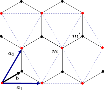
Figure 1: A honeycomb lattice described as a triangular Bravais lattice with a basis.

The model that we are going to study in this section is a variation of a model introduced in Ref. [48]. It features $S=1/2$ spins on each site of a honeycomb lattice, and shows exact dimensional reduction despite having non-commuting operators in its Hamiltonian.

The honeycomb lattice can be described as a triangular Bravais lattice, generated by the primitive vectors ${\bm{a_{1}}}={\bm{e_{1}}}$ and ${\bm{a_{2}}}=({\bm{e_{1}}}+\sqrt{3}{\bm{e_{2}}})/2$ (${{\bm{e_{1}}}}$ and ${{\bm{e_{2}}}}$ are the standard unit vectors of a square lattice), together with a basis described by the two vectors $\bm{0}$ and $\bm{b}=({\bm{e_{1}}}+({\bm{e_{2}}}/\sqrt{3}))/2$, see Fig. 1. The sites of the lattice are spanned by the sets of points ${\bm{m}}=m^{1}{\bm{a_{1}}}+m^{2}{\bm{a_{2}}}$, and the set $\bm{m^{\prime}}={\bm{m}}+\bm{b}$, with $m^{1},m^{2}\in\mathbb{Z}$. Imposing periodic boundary conditions amounts to identifying two sites ${\bm{m}}_{1},{\bm{m}}_{2}$ to be the same if their coordinates $m^{\mu}_{1},m^{\mu}_{2}$ are equal up to a multiple of the period $L_{\mu},\ \mu=1,2$; and we identify two sites ${\bm{m}}_{1}^{\prime},{\bm{m}}_{2}^{\prime}$ if ${\bm{m}}_{1}^{\prime}-\bm{b},{\bm{m}}_{2}^{\prime}-\bm{b}$ satisfy the same condition. The result is a honeycombl lattice $\Lambda^{P}_{\sf hex}$ with the topology of a two-dimensional torus. Since we can associate each elementary hexagon to a site ${\bm{m}}$ in the triangular sublattice, we can use ${\bm{m}}$ as an index to label the two plaquette operators

$$W_{(1,{\bm{m}})}=\sigma^{z}_{\bm{m}}\sigma^{x}_{\bm{m^{\prime}}}\sigma^{y}_{{\bm{m}}+{\bm{a_{2}}}}\sigma^{z}_{\bm{m^{\prime}}+{\bm{a_{2}}}-{\bm{a_{1}}}}\sigma^{x}_{{\bm{m}}+{\bm{a_{2}}}-{\bm{a_{1}}}}\sigma^{y}_{\bm{m^{\prime}}-{\bm{a_{1}}}}\ ,$$

$$W_{(2,{\bm{m}})}=\sigma^{z}_{\bm{m}}\sigma^{y}_{\bm{m^{\prime}}}\sigma^{x}_{{\bm{m}}+{\bm{a_{2}}}}\sigma^{z}_{\bm{m^{\prime}}+{\bm{a_{2}}}-{\bm{a_{1}}}}\sigma^{y}_{{\bm{m}}+{\bm{a_{2}}}-{\bm{a_{1}}}}\sigma^{x}_{\bm{m^{\prime}}-{\bm{a_{1}}}}\ .$$ (64)

where $\sigma^{\alpha}_{\bm{m}}$ with $\alpha=x,y,z$ are Pauli matrices. Notice that any two of these plaquette operators commute, $[W_{(\mu,{\bm{m}})},W_{(\nu,\bm{n})}]=0$.

The honeycomb extended toric code (HETC) model that we will study is specified by the Hamiltonian

$$H_{\sf HETC}=-\sum_{\mu=1,2}\sum_{{\bm{m}}\in\Lambda^{P}_{\sf hex}}\ J_{\mu}\,W_{(\mu,{\bm{m}})}-h\sum_{m^{1}=1}^{L_{1}-1}\sum_{m^{2}=1}^{L_{2}}\sigma^{z}_{\bm{m}},$$ (65)

illustrated in Fig. 2 for a lattice with periods $L_{1}=3,\ L_{2}=2$. The Hamiltonian acts on a Hilbert space of dimension $(2^{N_{s}})^{2}=2^{2N_{s}}$, with $N_{s}=L_{1}L_{2}$. If $h=0$, $H_{\sf HETC}$ reduces to the model introduced in Ref. [48]. Notice that the magnetic field $h$ is staggered, meaning that it is zero on all sites ${\bm{m}}^{\prime}$, and that it is mostly homogeneous, except for the (one-dimensional) circle of sites $L_{1}{\bm{a_{1}}}+m^{2}{\bm{a_{2}}},\ m^{2}=1,\cdots,L_{2}$, where it is also zero. The Hamiltonian $H_{\sf HETC}$ is self-dual under the exchange $J_{1}\leftrightarrow J_{2}$, but we will not show this directly, as it will become clear after the duality to a ${\bf d}=1$ model.

We will use the new approach to dualities developed in Refs. [1] to look for dual representations of $H_{\sf HETC}$. Consider the elementary operators $W_{(\mu,{\bm{m}})}$ and $\sigma^{z}_{\bm{m}}$, and only those operators. It is convenient to have a uniform denomination for them, and so we agree to call them generically bonds [18]. The bonds of a Hamiltonian (like $H_{\sf HETC}$) generate a model-specific bond algebra of interactions that has typically a very different structure as compared to the algebra of elementary degrees of freedom (spins $S=1/2$ in the case at hand). So it was proposed in [1] to look for dualities as structure-preserving mappings (homomorphisms, or isomorphisms in the absence of gauge symmetries) of bond algebras local in the bonds. To find a dual representation of $H_{\sf HETC}$ we need to characterize its bond algebra, and find a model $H_{\sf HETC}^{D}$ that looks different but has in fact a bond algebra isomorphic to that of $H_{\sf HETC}$.

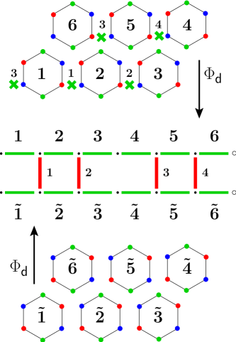
Figure 2: Honeycomb lattice with $L_{1}=3,\ L_{2}=2$, and periodic boundary conditions (twelve distinct sites). The top panel shows the plaquette bonds $W_{(1,{\bm{m}})}$ introduced in Eq. (6.1), numbered from one to six, and the four transverse fields $\sigma^{z}$ as green crosses (the spin labelled as three is not part of the Hamiltonian, but it appears in one of its ${\bf d}$-GLSs). The bottom panel shows the plaquette bonds $W_{(2,{\bm{m}})}$. The green (blue, red) dots stand for spins $\sigma^{z}$ ($\sigma^{x},\ \sigma^{y}$). The middle panel represents the dual, one-dimensional ladder model defined in Eq. (67). The duality mapping $\Phi_{{\sf d}}$ defined in Eq. (68) is indicated by corresponding labels in the illustrations of both models. For example, the plaquette bond in the bottom panel labelled as $\tilde{1}$ maps to the link $\sigma^{z}_{2,1}\sigma^{z}_{2,2}$ indicated by a green horizontal bar, and labelled by $\tilde{1}$ as well. The dual model satisfies periodic boundary conditions.

Since each bond $\sigma^{z}$ anticommutes with four plaquettes, $H_{\sf HETC}$’s bond algebra is non-commutative. The bonds $W_{(\mu,{\bm{m}})}$ commute with each other, and satisfy the constraints

$$\prod_{\bm{m}}\ W_{(\mu,{\bm{m}})}=\mathds{1},\ \ \ \ \mu=1,2.$$ (66)

Keeping these relations and constraints in mind, one can check that the bonds for a one-dimensional ladder of spins with periodic boundary conditions satisfy identical relations and constraints, as illustrated in Fig. 2. It follows that $H_{\sf HETC}$ is dual to

$$H_{\sf HETC}^{D}=-\sum_{\mu=1,2}\sum_{m=1}^{N_{s}}\ J_{\mu}\sigma^{z}_{\mu,m}\sigma^{z}_{\mu,m+1}-h\sum_{s=0}^{L_{2}-2}\sum_{i=2}^{L_{1}-1}\sigma^{x}_{1,i+s(L_{1}-1)}\sigma^{x}_{2,i+s(L_{1}-1)}.$$ (67)

This establishes the one-dimensional character of $H_{\sf HETC}$. The self-dualities of that Hamiltonian follow from those of the Ising ladder.

It will be useful in the following to have an explicit description of the duality mapping connecting the two models of Eqs. (65, 67). First, we number the sites of the honeycomb lattice as in Fig. 3. The duality mapping then reads

$$W_{(\mu,{\bm{m}})} \ \stackrel{{\scriptstyle\Phi_{{\sf d}}}}{{\longrightarrow}}\ \sigma^{z}_{\mu,\phi({\bm{m}})}\sigma^{z}_{\mu,\phi({\bm{m}})+1},$$ (68)

$$\sigma^{z}_{\bm{m^{\prime}}} \ \stackrel{{\scriptstyle\Phi_{{\sf d}}}}{{\longrightarrow}}\ \sigma^{x}_{1,\phi(\bm{m^{\prime}})+1}\sigma^{x}_{2,\phi(\bm{m^{\prime}})+1},$$

so that $\Phi_{{\sf d}}(H_{\sf HETC})=H_{\sf HETC}^{D}$, see Fig. 2. The theory of operator algebras guarantees that isomorphisms like $\Phi_{{\sf d}}$ of Eq. (68) must be equivalent to a unitary transformation [1]. It follows that there is a unitary transformation $\mathcal{U}_{{\sf d}}$ such that $H_{\sf HETC}^{D}=\Phi_{{\sf d}}(H_{\sf HETC})=\mathcal{U}_{{\sf d}}H_{\sf HETC}\mathcal{U}_{{\sf d}}^{\dagger}$.

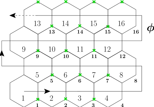
Figure 3: Numbering function $\phi$ used to describe the duality between $H_{\sf HETC}$ and a one-dimensional model, illustrated for a lattice with $L_{1}=4$ and $L_{2}>4$. $\phi$ numbers the hexagons, or equivalently, the sites of the underlying triangular Bravais lattice (large numbers). Since there is one point of the basis per hexagon, $\phi$ numbers these as well (small numbers). The green crosses represent the transverse-field bonds $\sigma^{z}$ present in $H_{\sf HETC}$. Periodic boundary conditions are considered.

The Hamiltonian $H_{\sf HETC}$ displays ${\bf d}=1$-GLSs that map into symmetries of the dual ladder model. Consider for concreteness the model illustrated in Fig. 2. It is clear that the operator

$$\sigma^{z}_{1}\sigma^{z}_{2}\sigma^{z}_{3}$$ (69)

(using the numbering of spins described in Fig. 2) commutes with $H_{\sf HETC}$. To determine the dual symmetry operator $\Phi_{{\sf d}}(\sigma^{z}_{1}\sigma^{z}_{2}\sigma^{z}_{3})$ we need to compute $\Phi_{{\sf d}}(\sigma^{z}_{3})$, which can be done according to the techniques of Ref. [1]. The result reads

$$\Phi_{{\sf d}}(\sigma^{z}_{3})=\sigma^{y}_{1,2}\sigma^{y}_{2,2}\sigma^{y}_{1,3}\sigma^{y}_{2,3},$$ (70)

so that the dual symmetry reduces to

$$\Phi_{{\sf d}}(\sigma^{z}_{1}\sigma^{z}_{2}\sigma^{z}_{3})=\sigma^{z}_{1,2}\sigma^{z}_{2,2}\sigma^{z}_{1,3}\sigma^{z}_{2,3}.$$ (71)

The calculation of the last paragraph allows us to understand the restrictions on the transverse-field bonds $\sigma^{z}$ allowed in $H_{\sf HETC}$. That is, the second term in Eq. (65) included a sum over only one triangular sublattice. The introduction of omitted bonds such as $\sigma^{z}_{3}$ on the other sublattice would destroy the exact dimensional reduction. To see this, notice that for a model with $L_{1},L_{2}$ arbitrary, the duality maps $\sigma^{z}_{L_{1}{\bm{a_{1}}}+{\bm{a_{2}}}+\bm{b}}$ to

$$\Phi_{{\sf d}}(\sigma^{z}_{L_{1}{\bm{a_{1}}}+{\bm{a_{2}}}+\bm{b}})=\prod_{i=2}^{L_{1}}\sigma^{y}_{1,i}\sigma^{y}_{2,i}.$$ (72)

(Equation (70) is a special case of this result, and similar expressions hold for $\Phi_{{\sf d}}(\sigma^{z}_{L_{1}{\bm{a_{1}}}+s{\bm{a_{2}}}+\bm{b}}),\ s=2,\cdots,L_{2}$). So, not only the presence of $\sigma^{z}_{L_{1}{\bm{a_{1}}}+{\bm{a_{2}}}+\bm{b}}$ in $H_{\sf HETC}$ would introduce long-range interactions in $H_{\sf HETC}^{D}$, but the range of these interactions would grow without bound as a function of the area on which $H_{\sf HETC}$ operates. This would spoil the exact dimensional reduction in the thermodynamic limit. In contrast, adding these bonds does not affect the d$=1$-GLSs of the model. This shows that d-GLSs can exist even in the absence of exact dimensional reduction, as already anticipated in the introduction.

The same crucial feature can be seen from a different perspective. It is intuitively clear that for any $D$-dimensional model one can always devise artificially a dual, lower-dimensional, model. What sets most of these dualities apart from true exact dimensional reduction is again that the range of the interactions in the lower-dimensional model will in general grow without bound as a function of the size of the higher-dimensional model. Only dualities that fail to show this feature establish exact dimensional reduction.

Thus, we conclude this section by highlighting its important result: the mapping of the $D=2$ quantum system of Eq. (65) on a honeycomb lattice, with a staggered field appearing only on one triangular sublattice, into the $d=1={\bf d}$ (ladder) short-range system of Eq. (67).

6.2 Topological color codes

We next briefly remark on dimensional reduction in the case of color codes [49]. The discussion will be very similar to that in previous section.

Color codes are defined on planar graphs such that three and only three links meet at any site of the graph (trivalent graphs), and such that any plaquette is bounded by an even number of links. There are two stabilizers per plaquette $p$: $B_{p}^{\alpha}=\prod_{i\in p}\sigma_{i}^{\alpha}$ with $\alpha=x$ or $z$. Thus, the operators $B_{p}^{x,z}$ are products of spins $S=1/2$ at lattice sites that belong to a given plaquette. The total Hamiltonian is given by a sum of these operators (bonds) over all plaquettes

$$H_{\sf TCC}=-\sum_{p}B^{x}_{p}-\sum_{p}B^{z}_{p}.$$ (73)

We will not repeat the calculations explicitly for this model, they are analogous to those carried out for the model investigated in Section 6.1 and the $D=3$ model to be investigated in the next section, Section 6.3. Since, by definition of the lattice supporting a color code, all plaquettes share an even number of common sites [49], the bonds $B_{p}^{\alpha}$ and $B_{p^{\prime}}^{\alpha^{\prime}}$ commute always,

$$[B_{p}^{\alpha},B_{p^{\prime}}^{\alpha^{\prime}}]=0,$$ (74)

for all $p,p^{\prime},\alpha,$ and $\alpha^{\prime}$, and

$$(B_{p}^{\alpha})^{2}=\mathds{1}.$$ (75)

If the lattice is realized on the surface of a torus, the bond algebra is supplemented by two additional relations (aside from Eqs. (74, 75)). These are given by

$$\prod_{p}B_{p}^{\alpha}=\mathds{1},$$ (76)

for $\alpha=x,$ and $z$. That is, the product of all operators $B_{p}^{x}$ over all plaquettes $p$ is unity (and the same holds true for the product of all stabilizer operators $B_{p}^{z}$). The system of Eqs. (73, 74, 75, 76) is defined on a Hilbert space of dimension $2^{N_{s}}$ with $N_{s}$ the number of sites of the system. The problem, as formulated, has a bond algebra isomorphic to that of two decoupled, periodic Ising chains in zero transverse field (see Ref. [2] for an analogous duality for the toric code model). Thus, this system has an identical spectrum to two independent, periodic classical Ising chains.

Color codes have d$=1$-GLSs. In particular, the toric color code just described commutes with any string operator obtained by multiplying all the spins $\sigma^{x}$ or all the spins $\sigma^{z}$ on the links of any closed curve [49].

6.3 The XXYYZZ model

Our third example of dimensional reduction entails a system that we call the XXYYZZ model [50]. It can be described in terms of $S=1/2$ spins placed on sites ${\bm{m}}$ of an fcc Bravais lattice. For concreteness, we can describe the sites ${\bm{m}}=m^{1}{\bm{a_{1}}}+m^{2}{\bm{a_{2}}}+m^{3}{\bm{a_{3}}}$, $m^{\mu}\in\mathbb{Z}$ with $\mu=1,2,3$, as linear combinations of the basis vectors, as illustrated in Fig. 4,

$${\bm{a_{1}}}=\frac{{\bm{e_{2}}}+{\bm{e_{3}}}}{2},\ \ {\bm{a_{2}}}=\frac{{\bm{e_{3}}}+{\bm{e_{1}}}}{2},\ \ {\bm{a_{3}}}=\frac{{\bm{e_{1}}}+{\bm{e_{2}}}}{2}.$$ (77)

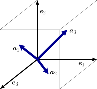
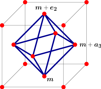
Figure 4: The basis vectors ${\bm{a_{1}}},{\bm{a_{2}}},{\bm{a_{3}}}$ for the fcc Bravais lattice. For any site ${\bm{m}}$ in an fcc lattice, there is one and only one octahedron with ${\bm{m}}$ as its lowest vertex.

The distinguishing feature of the fcc lattice that we would like to exploit is the fact that it has exactly one elementary octahedron per lattice site. In other words, for any site ${\bm{m}}$ of the fcc lattice, there is exactly one elementary octahedron having ${\bm{m}}$ as, say, its lowest vertex (and with every other vertex in the lattice as well). Then, we can introduce the operator

$$O_{\bm{m}}=\sigma^{x}_{{\bm{m}}+{\bm{a_{1}}}-{\bm{a_{2}}}}\sigma^{x}_{{\bm{m}}+{\bm{a_{3}}}}\sigma^{y}_{{\bm{m}}}\sigma^{y}_{{\bm{m}}+{\bm{e_{2}}}}\sigma^{z}_{{\bm{m}}+{\bm{a_{3}}}-{\bm{a_{2}}}}\sigma^{z}_{{\bm{m}}+{\bm{a_{1}}}},$$ (78)

associated with each site in the lattice (notice that ${\bm{e_{1}}},{\bm{e_{2}}},{\bm{e_{3}}}$ are integral combinations of ${\bm{a_{1}}},{\bm{a_{2}}},{\bm{a_{3}}}$, and so they represent displacements in the fcc lattice, even though they do not form a basis). In other words, the interaction terms are given by the product of all sites surrounding a given site of the even sublattice with the product being of the form “XXYYZZ” wherein the component of the spin appearing in the product is determined by its location relative to the center of the octahedron formed by the six sites. This constitutes a $D=3$ generalization of the “XXYY” product appearing in Wen’s $D=2$ model [35] (that is also dual to Kitaev’s Toric code model [19]).

Next, we introduce periodic boundary conditions in all three directions ${\bm{a_{1}}},{\bm{a_{2}}},{\bm{a_{3}}}$, to obtain a finite fcc lattice $\Lambda^{P}_{\sf fcc}$ with the topology of a three-dimensional torus. More specifically, we identify any two points ${\bm{m}}$ and ${\bm{m}}^{\prime}$ equal up to a multiple of the period $L_{\mu}$ in the $\bm{a_{\mu}}$ direction. The fcc structure forces the periods $L_{\mu}$ to be even integers as should become clear below (see Fig. 5). The Hamiltonian of the XXYYZZ model reads

$$H_{\sf XXYYZZ}=-J\sum_{{\bm{m}}\in\Lambda^{P}_{\sf fcc}}\ O_{\bm{m}}.$$ (79)

This Hamiltonian acts on a state space of even dimension $2^{N_{s}}$, with $N_{s}=L_{1}L_{2}L_{3}$ an integer multiple of four, and displays d$=1$-GLSs that are described in Ref. [50]. Our goal is to employ the general techniques introduced in [1] to look for an exact duality of $H_{\sf XXYYZZ}$ to a lower-dimensional model.

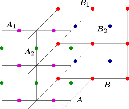
Figure 5: The fcc Bravais lattice can be built as an $ABAB$ stack of two square lattices ($A$ and $B$), displaced relative to each other (we show a lattice elongated in the stacking direction to make the figure more clear). Since the planar lattices $A$ and $B$ are both bipartite, the sites of an fcc lattice can be grouped into four disjoint classes. Any two octahedra belonging to sites in the same class share at most one vertex.

The XXYYZZ model shares several features of typical models displaying TQO: its bonds $O_{\bm{m}}$ commute with each other and the degeneracy of the ground energy level depends on the topology of the underlying lattice (that we have fixed to be toroidal here). The bonds $\{O_{\bm{m}}\ |\ {\bm{m}}\in\Lambda^{P}_{\sf fcc}\}$ generate a commutative bond algebra. We saw already that dualities are encoded in the structure of this bond algebra, so we need to specify it completely. The extra information we need is that, by virtue of the periodic boundary conditions, the bonds $O_{\bm{m}}$ satisfy four constraints.

To understand this, notice that we can split the sites of an fcc lattice into four disjoint classes (at least for periodic and open boundary conditions). The reason is that, as shown in Fig. 5, the fcc lattice can be constructed as a stack $ABAB$ of bipartite square lattices $A,\,B$ displaced relative to each other. Thus we can distinguish four types of sites, according to whether they belong to the sublattice $A_{1}$ or $A_{2}$ of an $A$ plane, or $B_{1}$ or $B_{2}$ of a $B$ plane (see Fig. 5). On the other hand, the bonds $O_{{\bm{m}}_{\kappa}}$ in any one class $\kappa=A_{1},A_{2},B_{1}$, or $B_{2}$ share exactly one site with its neighbors in the same class (and the corresponding spin, see Eq. (78)). It follows that

$$\prod_{{\bm{m}}_{\kappa}}\ O_{{\bm{m}}_{\kappa}}=\mathds{1}.$$ (80)

These are the four constraints that complete the specifications of the commutative bond algebra for $H_{\sf XXYYZZ}$.

As explained in Sec. 6.1, a Hamiltonian will be dual to $H_{\sf XXYYZZ}$ if the two models share bond algebras with identical structures (isomorphic bond algebras), and act on state spaces of the same dimension. Let us consider then the model

$$H_{\sf 4IP}=-J\sum_{\kappa=1}^{4}\sum_{m=1}^{N_{s}/4}\sigma^{z}_{\kappa,m}\sigma^{z}_{\kappa,m+1},$$ (81)

that represents four independent (decoupled), periodic Ising chains. The bond algebra generated by the set of bonds $\{\sigma^{z}_{\kappa,m}\sigma^{z}_{\kappa,m+1}\ |\ \kappa=1,2,3,4;\ m=1,\cdots,N_{s}/4\}$ is characterized by the fact that all bonds commute, and satisfy four independent constraints

$$\prod_{m=1}^{N_{s}/4}\ \sigma^{z}_{\kappa,m}\sigma^{z}_{\kappa,m+1}=\mathds{1},\ \ \ \ \forall\kappa.$$ (82)

Also, $H_{\sf 4IP}$ acts on a state space of dimension $(2^{N_{s}/4})^{4}=2^{N_{s}}$. It follows that $H_{\sf 4IP}$ is dual (unitarily equivalent) to $H_{\sf XXYYZZ}$. To establish a duality mapping, let $\kappa=A_{1},A_{2},B_{1},B_{2}$ correspond to $\kappa=1,2,3,4$, and let $\phi_{\kappa}$ be any numbering of the sites ${\bm{m}}_{\kappa}$ in the sublattice $\kappa=A_{1},A_{2},B_{1},B_{2}$, from one to $N_{s}/4$. Then

$$O_{{\bm{m}}_{\kappa}}\ \stackrel{{\scriptstyle\Phi_{{\sf d}}}}{{\longrightarrow}}\ \sigma^{z}_{\kappa,\phi_{\kappa}({\bm{m}}_{\kappa})}\sigma^{z}_{\kappa,\phi_{\kappa}({\bm{m}}_{\kappa})+1}$$ (83)

is a duality isomorphism that maps $H_{\sf XXYYZZ}$ to $H_{\sf 4IP}$, i.e., $\Phi_{{\sf d}}(H_{\sf XXYYZZ})=\mathcal{U}_{{\sf d}}H_{\sf XXYYZZ}\mathcal{U}_{{\sf d}}^{\dagger}=H_{\sf 4IP}$. It follows that the XXYYZZ model must display exact one-dimensional behavior. Thus, in conclusion, we mapped the $D=3$ system of Eqs. (78, 79) on an fcc lattice to the $d=1={\bf d}$ system of Eq. (81) representing four decoupled Ising chains.

It is important to stress that the source of the dimensional reduction in these two last models is not the completely commutative structure of their bond algebras. For instance, a model as simple as the $D=2$ Ising model in zero magnetic field

$$H_{\sf I}=-\sum_{\mu=1,2}\sum_{\bm{r}}\ J_{\mu}\,\sigma^{z}_{\bm{r}}\sigma^{z}_{{\bm{r}}+\bm{e_{\mu}}},$$ (84)

with ${\bm{r}}=r^{1}{\bm{e_{1}}}+r^{2}{\bm{e_{2}}}$, $r^{\mu}\in\mathbb{Z}$, denoting the sites of a simple square lattice, displays a completely commutative bond algebra but no dimensional reduction, due to the presence of constraints

$$\mathds{1}=\sigma^{z}_{\bm{r}}\sigma^{z}_{{\bm{r}}+{\bm{e_{1}}}}\times\sigma^{z}_{{\bm{r}}+{\bm{e_{1}}}}\sigma^{z}_{{\bm{r}}+{\bm{e_{1}}}+{\bm{e_{2}}}}\times\sigma^{z}_{{\bm{r}}+{\bm{e_{1}}}+{\bm{e_{2}}}}\sigma^{z}_{{\bm{r}}+{\bm{e_{2}}}}\times\sigma^{z}_{{\bm{r}}+{\bm{e_{2}}}}\sigma^{z}_{\bm{r}}.$$

Notice also that the Ising model has no d-GLSs with ${\bf d}<2$.

6.4 Effective boundary theories

In the exact dimensional reduction mappings that we studied thus far in this section, the dimension of the Hilbert space was preserved. Thus, for instance, when mapping a two-dimensional system onto a one-dimensional one, the number of lattice sites was unaltered. By contrast, in Section 3, we illustrated how local boundary theories can be constructed wherein the system size was reduced; these local boundary theories, however, only provided bounds on the correlation functions and, generally, did not constitute exact duals to the original high-dimensional theory. In this brief subsection, we wish to briefly point out that in some cases local boundary theories can constitute exact duals to the bulk system. In such instances, the general approach of exact dualities that we considered earlier in Section 6 coincides with that of the boundary theories of Section 3.

Towards that end, we seek an effective Hamiltonian $H_{\sf eff}$ such that

$${\cal Z}={\sf Tr}_{\Lambda}(\exp(-\beta H))={\cal N}\ {\sf Tr}_{\Gamma}(\exp(-\beta H_{\sf eff})).$$ (85)

Here, $H$ denotes the full Hamiltonian of the $D$-dimensional system $\Lambda=\Gamma\cup\bar{\Lambda}$, whereas $H_{\sf eff}$ denotes an effective Hamiltonian on a $d$-dimensional boundary $\Gamma$. An overall normalization factor is indicated by ${\cal N}$.

In the quantum spin lattice models that we considered above, the trace on any set of chosen bulk fields (or bonds appearing in the Hamiltonian [18, 1]) can be done trivially. In the case of the system of Eq. (65) in the absence of an external field ($h=0$) as well as the systems of Sections 6.3, and 6.2, a partial trace over some of the bonds renders the remaining system to be that of decoupled bonds (or Ising spins in this case). In particular, the effective boundary theories that contain all bonds that have their support on $\Gamma$ alone is given by that of decoupled Ising spins,

$$H_{\sf eff}=-\sum_{{\bm{x}}\in\Gamma}\sigma^{z}_{{\bm{x}}}.$$ (86)

That is, the trace over the bulk fields $\bar{\Lambda}$ gives rise to a Hilbert space volume factor alone that multiplies the partition function associated with $H_{\sf eff}$ of Eq. (86). Now, the theory of Eq. (86) were to result from the system of Eq. (65) in the absence of an external field ($h=0$) and the systems of Sections 6.3 and 6.2, if we were to “freeze” out the bulk spins in a spirit similar to that the derived local bounding boundary theories of Section 3.

7 Consequences of dimensional reduction: limits on the storage of quantum information

In general, we may apply the bounds of [2, 3] to arrive at both upper and lower bounds on all correlation lengths and autocorrelation times in general systems with $\bf d$-GLSs. In particular, these bounds on autocorrelation times provide limitations on quantum memory schemes and illustrate that, in some cases such as that of Kitaev’s toric code system [19], information will be lost after a period that does not scale with the system size.

Kitaev’s toric code model is a $D=2$ system defined on a torus (as the name suggests) that exhibits a ${\bf d}=1$ $\mathbb{Z}_{2}\times\mathbb{Z}_{2}$ symmetry. The degrees of freedom in this model are spin $S=1/2$ operators $(\sigma_{ij}^{x}$ or $\sigma_{ij}^{z}$) on the links $(ij)$ of a square lattice having $|\Lambda|=N_{s}$ vertices that is endowed with periodic boundary conditions. (To conform with the standard conventions, we denote the links by $(ij)$ rather than the particular dual lattice site on which they are centered.) Specifically, this model [19] is defined by the Hamiltonian

$$H_{\sf Kitaev}=-\sum_{s=1}^{N_{s}}A_{s}-\sum_{p=1}^{N_{s}}B_{p},$$ (87)

with the star and plaquette operators $A_{s}$ and $B_{p}$ given by

$$A_{s}=\prod_{j}\sigma_{js}^{x},~{}\ B_{p}=\prod_{(ij)\in p}\sigma_{ij}^{z}.$$ (88)

In the first of Eqs. (88), $j$ denotes all nearest neighbors of $s$. In Kitaev’s model, information is stored in two “topological qubits” determined by the eigenvectors of the ${\bf d}=1$ symmetry operators

$$Z_{1,2}=\prod_{(ij)\in C_{1,2}}\sigma^{z}_{ij},~{}~{}X_{1,2}=\prod_{(ij)\in C^{\prime}_{1,2}}\sigma^{x}_{ij},$$ (89)

where $C_{1}(C_{2}^{\prime})$ are horizontal and $C_{2}(C_{1}^{\prime})$ vertical closed (${\bf d}=1$) contours on the lattice (dual lattice) on the torus. As illustrated in [2], Kitaev’s model is special in that it may be exactly mapped to two decoupled classical Ising chains (i.e., a system of dimension $d={\bf d}=1$). Such a mapping is performed along lines similar to those of Section 6. The operators $A_{s}$ and $B_{p}$ map onto bonds of the two decoupled Ising chains (each of length $N_{s}$). The mapping is achieved by replacing, in the sum of Eq. (87), $A_{s}\to\sigma^{z}_{s}\sigma^{z}_{s+1}$ on one chain and $B_{p}\to\tau^{z}_{p}\tau^{z}_{p+1}$ on the other chain. That is, the Hamiltonian of the $D=2$ dimensional system of Eq. (87) is dual to that of two Ising chains ($d={\bf d}=1$)

$$H_{{\sf{2}\sf{Ising-chain}}}=-\sum_{s=1}^{N_{s}}\sigma^{z}_{s}\sigma^{z}_{s+1}-\sum_{p=1}^{N_{s}}\tau^{z}_{p}\tau^{z}_{p+1},$$ (90)

with $\sigma^{z}_{N+1}=\sigma^{z}_{1}$ and $\tau^{z}_{N+1}=\tau^{z}_{1}$. Similarly, within this mapping, the topological qubits $Z_{1}$ and $Z_{2}$ map onto single spins (say those located at the sites number 1 on both chains), $Z_{1}\to\sigma^{z}_{1}$ and $Z_{2}\to\tau^{z}_{1}$. The above set of mappings preserves all of the algebraic relations amongst the bonds $\{A_{s}\}$ and $\{B_{p}\}$ that appear in the Hamiltonian of Eq. (87) as well as the two qubits $Z_{1}$ and $Z_{2}$.

We now discuss consequences of dimensional reduction on the storage of quantum information. First, we very briefly discuss how, physically, information may be lost by defects in this particular example system of Kitaev’s model. Then, we turn to a formal framework that illustrates how bounds on the storage of quantum information follow from our EQDR theorem. Lastly, we remark how such dimensional reductions allow for an understanding of particular cross-over temperatures in finite size systems.

Conceptually understanding how dimensional reduction, when it occurs, may limit the storage of quantum information is relatively straightforward when thought about in terms of defects that eradicate the character of an initial stored state and lead to a finite correlation length. In Kitaev’s toric code model, dimensional reduction implies that topological defects that arise in one-dimensional Ising systems rear their head anew on the $D=2$ torus. Similar considerations apply for the other systems discussed in Section 6. In an Ising chain the proliferation of domain walls leads, at any positive temperature, to a finite correlation length and to finite autocorrelation (or memory) times. In accord with the one-dimensional character, the low temperature autocorrelation times may scale as $\tau\sim\exp[\beta\Delta]$ where $\Delta$ is an energy penalty associated with a domain wall. In a one-dimensional Ising chain with exchange constant $J$, this penalty is system size ($N_{s}$) independent and set solely by the energy scale $J$. (In Eq. (90), the nearest-neighbor exchange constant $J=1$.) Thus, any information that is initially stored in Kitaev’s toric code model will, at sufficiently long times, be destroyed by thermal fluctuations [2].

We now step back to consider the more general consequences of effective dimensional reductions borne by symmetries (Section 3). (In Kitaev’s toric code model that exhibits the ${\bf d}=1$ GLSs of Eqs. (89) as well as other systems in Section 6, these effective dimensional reductions become exact.) To obtain bounds on memory times, we set the operator function $f$ of Section 3 to represent an autocorrelation function. That is, we consider what occurs when we choose $f=Z_{1}(0)Z_{1}(t)$ so that its expectation value will measure the autocorrelation of an initial quantity $Z_{1}$ with itself at later times $t$. If quantum memories are stable then $\langle f\rangle^{D}$ does not decay at long times. By the results of Section 3, the autocorrelation function in a general system with ${\bf d}$-GLSs, is bounded (both from above and from below) by autocorrelation functions of a $d$-dimensional system in which the range of the interactions and symmetries are preserved

$$G_{\sf lower}^{(2)}\leq G^{(2)}(t)\equiv\langle Z_{1}(0)Z_{1}(t)\rangle\leq G_{\sf upper}^{(2)},$$ (91)

with $G_{\sf lower}^{(2)},G_{\sf upper}^{(2)}$ autocorrelation functions in a $d$-dimensional system. These lower-dimensional autocorrelation functions serve as upper and lower bounds on the autocorrelation function in $D$ spatial dimensions. It is notable that in systems with interactions of finite range and strength the autocorrelation times of quantities not invariant under ${\bf d}=1$ GLSs do not scale with the system size. Thus, in such systems, the autocorrelation times are system size independent. In a similar fashion, system size dependent autocorrelation times appear in the ordered phase of low-dimensional systems with long-range interactions exhibiting a phase transition, such as ferromagnetic spin chains with $1/r^{\lambda}$ interactions ($\lambda\leq 2$) [53]. Taken together with the bounds of Section 3, this allows for divergent autocorrelation times of quantities that are not invariant under ${\bf d}$-GLS in systems having long-range interactions. It is notable that even though excitations may involve a macroscopic number of spatially local degrees of freedom in systems such as Kitaev and the XXYYZZ model, and thus it might be expected that the system exhibits glass-like characteristics [50], what matters in the computation of the autocorrelation functions is not how memory may be erased in real space. Rather, what is of importance, so long as the noise is random, is the algebra underlying these excitations. Thus, we would like to suggest that, at least for some realizations of noise stemming from an external heat bath, the XXYYZZ model exhibits one-dimensional memory type effects and not glass-like features.

A peculiar feature of Kitaev’s toric code model is the existence of a cross-over temperature which scales with the system size [2, 54]. In what follows, we discuss this observation through the prism of the exact dimensional reduction to Ising chains that Kitaev’s model displays. In an Ising chain with nearest-neighbor interactions (of strength $J=1$) at an inverse temperature $\beta$, the correlation length scales as $\xi\sim-1/\ln(\tanh\beta)$. This scaling implies the existence of a crossover temperature scale $T_{\sf cross}$ below which the entire chain is correlated and above which the chain length is larger than the correlation length. On a single Ising chain with $N_{s}\gg 1$ spins, this gives rise to a crossover temperature $T_{\sf cross}\sim 1/\ln N_{s}$ [2]. A similar crossover temperature is seen when the entanglement entropy is analyzed [54]. A rudimentary understanding of this scaling can be seen from standard energy-entropy balance considerations in the free energy, $F=E-T{\sf S}$, for the insertion of a ${\bf d}=1$ defect (i.e., a domain wall in a one-dimensional chain for discrete ${\bf d}=1$ symmetries) in a system with short-range interactions. Associated with the insertion of a defect there is an energy penalty $E=\Delta$ and an entropy ${\sf S}\sim\ln N_{s}$. These two contributions lead to a a crossover temperature scaling as $T_{\sf cross}\sim 1/\ln N_{s}$. For $T<T_{\sf cross}$ defects are unfavorable, while $T>T_{\sf cross}$ defects proliferate. The discussion above can replicated mutatis mutandis for the systems of Section 6 when these reduce to Ising chains as well as many others which reduce to other low-dimensional systems. The existence of predicted crossover temperatures in these systems, as adduced from our general considerations above regarding dimensional reductions, may hopefully be bolstered by explicit computations of thermodynamic quantities [2] or entanglement entropy [54] in future works.

8 Conclusions

In conclusion, we examined both (i) effective and (ii) exact dimensional reductions and holographic correspondences. Specifically, we proved that

(i) In a rather general local $D$-dimensional quantum theory that is defined on some volume $\Lambda$, correlation functions involving fields that lie on a subspace $\Gamma\subset\Lambda$ of dimension $d<D$ can generally be bounded by correlation functions in a local $d$-dimensional theory. These bounds lead to an effective dimensional reduction which become most potent when the original $D$-dimensional theory exhibits a particular symmetry (or set of symmetries) having its support on the region $\Gamma$. (A symmetry operator that has its support on a general region of dimension ${\bf d}$ is termed a ${\bf d}$-dimensional gauge-like symmetry.) When the symmetry operator acts on the ${\bf d}=d$ spatial region $\Gamma$, the resulting bounds of Eq. (35) lead to a generalized quantum Elitzur theorem.

(ii) Stronger than effective dimensional reductions are exact dimensional reductions that relate systems in different dimensions. We studied and illustrated exact dimensional reductions of two different types:
(a) Dualities centered on the large-$n$ limit of $O(n)$ vector theories and the high temperature (or weak coupling) limit. The dualities derived in this case relied on the dependence of the partition function (or generating functional) on a local effective density (in the latter case, the density of states for single modes in the non-interacting limit which retains its character also in the presence of interactions in the large-$n$ limit or that of high temperatures). We briefly speculated that it may be possible to search for analogues of functional theory type treatments [36] in field theories and interacting many-body systems that effectively render the theory nearly non-interacting. With the aid of these functionals, it may be possible to more generally construct transformations that do not deform the appropriate functions and thus preserve the features of a local theory when it is related to another local system in a different spatial dimension.
(b) We further examined exact dualities that do not appear in some limit but that, rather, always hold true. The studied dimensional reduction dualities focused solely on the physical bonds that appear in the Hamiltonian or action defining the theories. With the aid of this approach, redundant degrees of freedom on both sides of a general duality (e.g., gauge symmetries in various gauge theories, local coordinate invariance in gravity theories, etc.) may be automatically discarded. The equivalences in case (ii) focus on the form of the spectrum of the theory: case (a) focuses on the local density of states (in, for instance, $k$-space) and (b) on mappings that trivially preserve the exact spectrum of the theory.

Both the (i) effective and (ii) exact dimensional reductions introduced in this work do not require an actual physical compactification of dimensions.

9 Acknowledgements

We are indebted to inspiring discussions with Pawel O. Mazur, and Emil Mottola at the Condensed matter meets gravity workshop in the Lorentz Institute, Leiden, in August 2007 and to illuminating interactions with Clifford M. Will and Emanuel Knill. We wish to thank Simin Mahmoodifar for a very careful reading of the manuscript and corrections. ZN is indebted to the National Science Foundation (DMR-1106293) for support. GO acknowledges partial support by the National Science Foundation under Grant No. 1066293 and the hospitality of the Aspen Center for Physics.

Appendix A Entanglement-based version of the EQDR theorem

We briefly describe a variant of the EQDR theorem that holds for arbitrary states $\rho$, at least if the Hilbert space of the system is finite-dimensional. The assumptions are again that we can treat the bulk and the boundary as distinguishable, $\mathcal{H}_{\Lambda}=\mathcal{H}_{\Gamma}\otimes\mathcal{H}_{\bar{\Lambda}}$, and that operators $f$ localized on $\Gamma$ have the form $f=f_{\Gamma}\otimes\mathds{1}_{\bar{\Lambda}}$. Then we can expand an arbitrary state operator $\rho$ as

$$\rho=\sum_{i}\lambda_{i}\,\rho_{\Gamma i}\otimes\rho_{\bar{\Lambda}i},$$ (92)

where $\rho_{\Gamma i},\rho_{\bar{\Lambda}i}$ are state operators, and $\lambda_{i}$ may be any real number, positive or negative such that $\sum_{i}\lambda_{i}=1$. Separable or unentangled states correspond to the case where all $\lambda_{i}$ happen to be positive. An entangled state is characterized by the presence of at least one negative coefficient in (92).

Let us first justify Eq. (92). Notice that an arbitrary Hermitian operator can be written as the difference of two positive operators, by virtue of the spectral decomposition theorem. If $O$ is Hermitian and $o_{i},P_{i}$ are its real eigenvalues and eigenprojectors, then

$$O=\sum_{i}o_{i}P_{i}=\sum_{i_{+}}o_{i_{+}}P_{i_{+}}-\sum_{i_{-}}|o_{i_{-}}|P_{i_{-}}=O^{+}-O^{-},$$ (93)

where the index $i_{+}\ (i_{-})$ varies over that subset of $i$’s for which $o_{i}$ is positive (negative). We can identify the real space of Hermitian linear transformations $J_{\Lambda}$ on $\mathcal{H}_{\Lambda}$ with the space $J_{\Gamma}\otimes J_{\bar{\Lambda}}$, where $J_{\Gamma}$ and $J_{\bar{\Lambda}}$, represent transformations on the boundary and bulk, respectively. Since these are finite dimensional spaces, it follows [31] that any Hermitian operator on $\mathcal{H}_{\Lambda}$, and any state operator $\rho$ in particular, can be written as a real linear combination

$$\rho=\sum_{i}O_{\Gamma i}\otimes O_{\bar{\Lambda}i}.$$ (94)

While there is no guarantee that the $O_{\Gamma i},O_{\bar{\Lambda}i}$ will be state operators, we can apply the decomposition of Eq. (93) to each $O_{\Gamma i},O_{\bar{\Lambda}i}$ to turn the expansion of Eq. (94) into an expansion in terms of products of positive operators. If we next normalize these positive operators, we get the expansion of Eq. (92), and we see that the $\lambda_{i}$, although real, need not be positive by virtue of the minus sign in Eq. (93).

We can now use Eq. (92) to compute inequalities of interest to dimensional reduction and holographies. If $f=f_{\Gamma}\otimes\mathds{1}_{\bar{\Lambda}}$ is an observable

$$L_{+}\langle f\rangle^{+}_{l}-L_{-}\langle f\rangle^{-}_{l}\leq{\sf Tr}_{\Lambda}(\rho f)\leq L_{+}\langle f\rangle^{+}_{u}-L_{-}\langle f\rangle^{-}_{u}.$$ (95)

where $L_{+}=\sum_{i_{+}}\lambda_{i_{+}}$, $L_{-}=\sum_{i_{-}}|\lambda_{i_{-}}|$ are both positive,

$$\langle f\rangle^{+}_{u}\equiv{\sf max}_{i_{+}}{\sf Tr}_{\Gamma}(\rho_{\Gamma i_{+}}f_{\Gamma}),\ \ \ \ \langle f\rangle^{-}_{u}\equiv{\sf min}_{i_{-}}{\sf Tr}_{\Gamma}(\rho_{\Gamma i_{-}}f_{\Gamma}),$$ (96)

and

$$\langle f\rangle^{+}_{l}\equiv{\sf min}_{i_{+}}{\sf Tr}_{\Gamma}(\rho_{\Gamma i_{+}}f_{\Gamma}),\ \ \ \ \langle f\rangle^{-}_{l}\equiv{\sf max}_{i_{-}}{\sf Tr}_{\Gamma}(\rho_{\Gamma i_{-}}f_{\Gamma}).$$ (97)

Notice that if the state $\rho$ is unentangled, then $L_{-}=0$ and $L_{+}=1$, and this version of the EQDR theorem, Eq. (95), comes remarkably close to the classical dimensional reduction theorem, as perhaps is to be expected. In general, the inequalities of Eq. (95) clearly illustrate another way of achieving effective dimensional reduction.

References

References

- [1] E. Cobanera, G. Ortiz, and Z. Nussinov, Phys. Rev. Lett. 104, 020402 (2010); E. Cobanera, G. Ortiz, and Z. Nussinov, Adv. in Phys. 60, 679 (2011).
- [2] Z. Nussinov and G. Ortiz, Proc. Natl. Acad. Sciences 106, 16944 (2009) and supporting information therein; Z. Nussinov and G. Ortiz, Ann. Phys. 324, 977 (2009); Z. Nussinov and G. Ortiz, Phys. Rev. B 77, 064302 (2008).
- [3] C. D. Batista and Z. Nussinov, Phys. Rev. B 72, 045137 (2005).
- [4] V. Cvetkovic, Z. Nussinov, and J. Zaanen, Philos. Mag. 86, 2995 (2006).
- [5] S. E. Sebastian et. al., Nature 441, 617 (2006).
- [6] T. Kaluza, Sitzungsber. Preuss. Akad. Wiss. Berlin. (Math. Phys.) 966 (1921); O. Klein, Zeitschrift fur Physik A Hadrons and Nuclei 37 (12) 895 (1926).
- [7] M. B. Green, J. H. Schwarz, and E. Witten, Superstring Theory (Cambridge University Press, Cambridge, 1987).
- [8] R. Langlands, Lecture Notes in Math. 170 (Springer Verlag, Berlin, 1970), pp. 18.
- [9] A. Kaptusin and E. Witten, arXiv:hep-th/0604151 (2006).
- [10] J. M. Maldacena, Adv. theor. Math. Phys. 2, 231 (1998). [Int. J. Theor. Phys. 38, 1113 (1999).]
- [11] S. S. Gusber, I. R. Klebanov, and A. M. Polyakov, Phys. Lett. B 428, 105 (1998).
- [12] E. Witten, Adv. Theor. Math. Phys. 2, 253 (1998).
- [13] O. Aharony, S. S. Guber, J. M. Maldacena, H. Ooguri, and Y. Oz, Phys. Rep. 323, 183 (2000).
- [14] H. Nastase, hep-th/0712.0689 (2007).
- [15] P. K. Kovtun, D. T. Son, and A. O. Starinets, Phys. Rev. Lett. 94, 111601 (2005).
- [16] Ch. P. Herzog, P. Kovtun, S. Sachdev, and D. T. Son, Phys. Rev. D 75, 085020 (2007).
- [17] D. T. Son, Phys. Rev. D 78, 046003 (2008); K. Balasubramanian and J. McGreevy, Phys. Rev. Lett. 101, 061601 (2008); M. Sakaguchi and K. Yoshida, J. Math. Phys. 49, 102302 (2008); J. L.B. Barbon and C. A. Fuertes, JHEP, 9 , 030 (2008); W. D. Goldberger, JHEP 3, 069 (2009).
- [18] Z. Nussinov and G. Ortiz, Phys. Rev. B 79, 214440 (2009).
- [19] A. Yu. Kitaev, Annals Phys. 303, 2 (2003).
- [20] X-G. Wen, Quantum Field Theory of Many-Body Systems (Oxford University Press, Oxford, 2004), and references therein.
- [21] C. Xu and J. Moore, Nucl. Phys. B 716, 487 (2005); C. Xu and J. Moore, Phys. Rev. Lett. 93, 047003 (2004).
- [22] Z. Nussinov and E. Fradkin, Phys. Rev. B 71, 195120 (2005).
- [23] R. D. Somma, C. D. Batista, and G. Ortiz, Phys. Rev. Lett. 99, 030603 (2007).
- [24] A. Einstein, B. Podolsky, and N. Rosen Phys. Rev. 47, 777 (1935).
- [25] E. Schrödinger, Naturwissenschaften 23, 807 (1935).
- [26] H. Barnum, E. Knill, G. Ortiz, and L. Viola, Phys. Rev. A 68, 032308 (2003); H. Barnum, E. Knill, G. Ortiz, R. Somma, and L. Viola, Phys. Rev. Lett. 92, 107902 (2004).
- [27] T. D. Newton and E. P. Wigner Rev. Mod. Phys. 21, 400 (1949); A. S. Wightman Rev. Mod. Phys. 34, 845 (1962).
- [28] I. Montvay and G. Muenster, Quantum Fields on a Lattice, Cambridge University Press (1994).
- [29] P. A. M. Dirac, Rev. Mod. Phys. 17, 195 (1945).
- [30] We are grateful to Clifford M. Will for a quick tutorial regarding this note. As is well appreciated, it is not possible to (easily) define in gravitational systems a simple Boltzmann type distribution. For instance, the classical covariant Hamiltonian as defined from the action vanishes identically. By contrast, the non-covariant Hamiltonian defined via a split of coordinates on a time slice can at times lead to a sensible results as in some early works on canonical quantum gravity (e.g., the ADM formulation [46]). However, determining the time-like coordinate can be problematic (e.g., Schwarzschild metric, where is time-like outside the horizon and space-like inside). In some specific instances, reasonable results are obtained notwithstanding (e.g., as the static character of the Schwarzschild geometry is static as it has a time translation symmetry), may be exploited to obtain the Hawking-Bekenstein temperature. Another difficulty originates from the fact that gravity has negative specific heat, rendering the standard rules about stability of fluctuations suspect. For example, when energy is removed from a star, it gets hotter. The more massive a black hole is, the cooler it is, hence the Hawking radiation is totally irrelevant for astrophysical black holes. It is for this reason that a black hole can never be in thermal equilibrium with an infinite heat bath, only with one of finite size. Thus, a number of standard thermodynamic rules no longer hold when gravity is present. (Fundamentally, this reflects the quintessential character of gravity as a long-range interaction with no negative mass particles.)
- [31] D. R. Farenick, Algebras of Linear Transformations, Springer Verlag (2001).
-
[32]
In principle, the same superselection rules applies to observables.
However, when computing an average we have that
and so even if an observable does not respect the superselection rule it will automatically be substituted for one that does, provided the state carries the correct quantum statistics.(98) - [33] S. Elitzur, Phys. Rev. D 12, 3978 (1975).
- [34] Z. Nussinov, C. D. Batista, and E. Fradkin, Int. Jour. Mod. Phys. B 20, 5239 (2006).
- [35] X.-G. Wen Phys. Rev. Lett. 90, 016803 (2003).
- [36] P. Hohenberg and W. Kohn, Phys. Rev. 136, B864 (1964).
-
[37]
Within a Feynman diagrammatic type approach
applied to the quartic theory of Eq. (41),
to order , only “tree” type diagrams survive.
The bare propagators are dressed by a self-energy correction
leading to where with the bare propagator mass and the
(zeroth-order) self-energy self-consistently given by
Now, here is a key point that we may invoke. Equation (99) is invariant under any permutation of the momenta:(99)
and any relabeling of their indices. In particular, if two theories satisfy Eq. (43) then they identically share the same self-energy of Eq. (99) and display the same propagators .(100) - [38] S. K. Ma, Rev. Mod. Phys. 45, 589 (1973).
- [39] H. E. Stanley, Phys. Rev. 176, 718 (1968).
- [40] T. H. Berlin and M. Kac, Phys. Rev. 86, 821 (1952).
- [41] Within the conventional definition of the spherical model, are scalar fields. In order to make the equivalence between the spherical model and large- vector theories more general, we define here a vectorial version of the spherical model.
- [42] S. K. Ma, Phys. Rev. A 10, 1818 (1974).
- [43] S. Chakrabarty and Z. Nussinov, Phys. Rev. B 84, 064124 (2011).
- [44] J. M. Soler, Phys. Rev. B 69, 195101 (2004).
- [45] S.-S. Lee, Nucl. Phys. B 382, 567 (2010).
- [46] R. Arnowitt, S. Deser, and C. Misner, Phys. Rev. 116, 1322 (1959).
- [47] Z. Nussinov, Phys. Rev. B 69, 014208 (2004).
- [48] L. Liang and Y. Yu, Commun. Theor. Phys. 55, 80 (2011).
- [49] H. Bombin and M. A. Martin-Delgado, Phys. Rev. Lett. 97, 180501 (2006).
- [50] C. Chamon, Phys. Rev. Lett. 94, 040402 (2005).
- [51] S. Bravyi, B. Leemhuis, and B. Terhal, New J. Phys. 12, 083039 (2010).
- [52] J. Kogut, L. Susskind, Phys. Rev. D 11, 395 (1975); E. Fradkin, L. Susskind, Phys. Rev. D 17, 2637 (1978).
- [53] P. W. Anderson, G. Yuval, and D. R. Hamann, Phys Rev B 1, 4464 (1970).
- [54] C. Castelnovo and C. Chamon, Phys. Rev. B 76, 184442 (2007).