Multi-Zone Models of Superbursts from Accreting Neutron Stars

Abstract

Superbursts are rare and energetic thermonuclear carbon flashes observed to occur on accreting neutron stars. We create the first multi-zone models of series of superbursts using a stellar evolution code. We self-consistently build up the fuel layer at different rates, spanning the entire range of observed mass accretion rates for superbursters. For all models light curves are presented. They generally exhibit a shock breakout, a precursor burst due to shock heating, and a two-component power-law decay. Shock heating alone is sufficient for a bright precursor, that follows the shock breakout on a short dynamical time scale due to the fall-back of expanded layers. Models at the highest accretion rates, however, lack a shock breakout, precursor, and the first power law decay component. The ashes of the superburst that form the outer crust are predominantly composed of iron, but a superburst leaves a silicon-rich layer behind in which the next one ignites. Comparing the model light curves to an observed superburst from 4U 1636-53, we find for our accretion composition the best agreement with a model at three times the observed accretion rate. We study the dependence on crustal heating of observables such as the recurrence time and the decay time scale. It remains difficult, however, to constrain crustal heating, if there is no good match with the observed accretion rate, as we see for 4U 1636-53.

1. Introduction

X-ray flares have been observed from accreting neutron stars that are similar to Type I X-ray bursts, but that are a thousand times more energetic and last up to a day. Normal bursts (e.g., Lewin et al. 1993; Strohmayer & Bildsten 2006) result from hydrogen and helium burning to carbon and, through a series of alpha captures, the $\alpha$p-process, and proton captures, the rp-process, to heavier elements (Schatz et al. 2001, 2003b). The long flares, named ‘superbursts’, are attributed to the runaway thermonuclear burning of carbon in a $100\,\mathrm{m}$ thick layer of ashes of normal bursts (Cumming & Bildsten 2001; Strohmayer & Brown 2002). The day long decay is explained as being the cooling time scale of a layer of that thickness (Cumming & Macbeth 2004). Because it takes typically about one year to build up this $100$ meter thick layer, superbursts are much rarer than regular bursts. The first superbursts have been discovered relatively recently: it was only after the launch of the BeppoSAX and RXTE observatories that enough exposure time was collected to be able to detect such rare events (Cornelisse et al. 2000; Strohmayer & Brown 2002). At the time of writing, $20$ (candidate) superbursts have been observed from 11 sources (see Keek & in ’t Zand 2008 for an overview, and Kuulkers 2009, Chenevez et al. 2011, in’t Zand et al. 2011 for recent discoveries).

Two types of superbursts are discerned based on the composition of the material that is accreted from the companion star. Most superbursters are thought to accrete hydrogen-rich material. Their superbursts are energetic, but the peak brightness does not reach the Eddington limit. Superbursts have been observed from 4U 0614+91 (Kuulkers et al. 2010) and 4U 1820-30 (Strohmayer & Brown 2002, and a candidate in’t Zand et al. 2011). These sources are so-called ultra-compact X-ray binaries (UCXBs). UCXBs have a binary period of less than $80$ minutes. In such a small orbit, stable mass transfer by Roche-lobe overflow can only occur from an evolved star that has lost its hydrogen envelope. The material accreted onto the neutron star, therefore, contains no hydrogen, but may contain helium. The superburst from 4U $1820-30$ reached the Eddington luminosity and displayed photospheric radius expansion. For 4U 0614+91 the onset of the superburst was not observed.

Most superbursting sources have a high accretion rate $\dot{M}$ of at least $10\%$ of the Eddington-limited rate $\dot{M}_{\mathrm{Edd}}$ at the time of the superburst. Exceptions are 4U 0614+91 with $\dot{M}\simeq 0.01\dot{M}_{\mathrm{Edd}}$ (Kuulkers et al. 2010), and 4U 1608-522 where the accretion rate at the time of the superburst was high, but where the average rate over the previous years was $\dot{M}\simeq 0.01\dot{M}_{\mathrm{Edd}}$ (Keek et al. 2008). The $\alpha$-parameter, the ratio of the accretion fluence between normal bursts and the fluence of a burst, is typically high: $\alpha\simeq 1000$ (in ’t Zand et al. 2003). This indicates a relatively large part of the accreted material is burned in a stable manner instead of in bursts, and this may be necessary to achieve high enough carbon fractions. No superbursts have been observed from sources that only have stable burning and no bursts, though lower limits on the possible recurrence time have been determined (Keek et al. 2006). Although bursts reduce the carbon content of the envelope in the production of heavy elements, it has been suggested that the heavy elements are necessary for reducing the thermal conductivity, insuring that the superburst ignition is reached at the observed depth in the envelope (Cumming & Bildsten 2001).

From fits of superburst-decay models to observed light curves (Cumming & Macbeth 2004), Cumming et al. (2006) deduce that superbursts ignite at a column depth of $y\simeq 10^{11}-10^{12}\,\mathrm{g\,cm^{-2}}$ in a layer with a carbon mass fraction of $X_{12}\simeq 20\%$. It is a challenge for models to explain these ignition column depths. The carbon mass fractions are higher than what one-dimensional models that include large nuclear networks predict to be present in the ashes of normal bursts (Woosley et al. 2004; Fisker et al. 2008). Cooper et al. (2006) suggest that the companion stars of superbursters donate material with a CNO content that is four times higher than solar.

Superbursts ignite close to the outer crust, and as such are sensitive to the thermal properties of the crust, which are not yet well understood (Brown 2004). In turn, the temperature of the crust depends on neutrino-cooling in the neutron star core, which is also ill-constrained. Therefore, superbursts provide an observational measure of the thermal properties of the outer crust, and constrain the physics in the crust and the core (Cumming et al. 2006; Page & Cumming 2005).

The start of the superburst was observed only in eight cases. In six of these, a short precursor burst is detected. For the other two superbursts, the data was not of sufficient quality to exclude the presence of a precursor, with the possible exception of 4U 1608-522, although the detection of the superburst onset must be regarded tentative for this source (Keek et al. 2008). Weinberg & Bildsten (2007) explain the precursor as the result of a shock generated by the superburst ignition. This shock travels outwards through the envelope and triggers the ignition of either a helium-rich layer or another carbon-rich layer. The resulting flash is observable as the precursor burst.

In this paper we create a series of one-dimensional models of the neutron star envelope, where for the first time we self-consistently build up a carbon-rich layer at rates similar to the observed accretion rates. We follow the carbon burning during several consecutive superbursts. The dependence of observable properties of the bursts on crustal heating is investigated. A possible hydrogen or helium-rich atmosphere is not modeled in this paper.

2. Neutron star envelope model

2.1. Stellar evolution code

We employ the one-dimensional hydrodynamics stellar evolution code KEPLER (Weaver et al. 1978). We use a version of KEPLER that differs from the version used in recent studies (e.g., Woosley et al. 2002, 2004; Heger et al. 2007) in the accretion scheme and the opacities that are used. We model the neutron star envelope on a one-dimensional Lagrangian grid in the radial direction, under the assumption of spherical symmetry. The grid points represent the boundaries between concentric shells, that each have a certain mass, chemical composition, temperature, density, luminosity and radial velocity. Alternatively, a model could be considered a local ‘wedge’ of the neutron star, that would be well-approximated in a plane-parallel geometry.

Zones are added and removed in order to maintain an optimal grid for resolving gradients in all quantities, such that temperature, density, and radius vary from one zone to the next by at least 10% and at most 25%. Furthermore, zones are not removed if they extend over $0.02$ in $\log y$, where $y$ is the column depth. The effects of different rezoning criteria was tested in a limited number of models; the most important calculated properties such as burst recurrence times and energetics varied by at most a few percent. The mass of each zone as well as the size of each time step are recorded, such that small values are not lost due to numerical precision.

We implicitly solve the equations of mass, energy, and momentum conservation (Weaver et al. 1978). The equation of state allows for (non-)degenerate and (non-)relativistic electrons.

To follow the chemical evolution we have the use of two networks of nuclear reactions. An adaptive network follows a large number of reactions among hundreds of isotopes (Woosley et al. 2004). Because this network is computationally expensive, most of our calculations only use an approximation network consisting of 19 isotopes (Weaver et al. 1978). It includes the carbon fusion reactions as well as photodisintegration. Comparison of superburst models created using either network shows a $3.3\%$ shorter recurrence time for the model with the approximation network, and a $3.1\%$ lower burst fluence. This indicates that the large network generates $0.2\%$ more energy per unit mass than the approximation network. There is no notable difference in the light curves.

We take into account neutrino energy loss (Itoh et al. 1996), radiative opacity (Iben 1975), and electron conductivity (Itoh et al. 2008).

We consider convection using the Ledoux criterion, as well as semiconvection and thermohaline mixing (e.g., Heger et al. 2000). The induced mixing of the chemical composition is implemented as a diffusive process using mixing-length theory (e.g., Clayton 1968). Rotation and magnetic fields are not considered in these models.

2.2. Accretion and decretion

Previous studies of X-ray bursts with the KEPLER code implemented accretion by increasing the pressure at the outer zone over time to simulate the build-up of a column of material (e.g., Woosley & Weaver 1984; Taam et al. 1996). When this pressure reached a certain value, an extra zone containing the accreted mass was added on top of the model. This induced a momentary reduction of the time step as well as an artificial dip in the light curve. In the present study we employ an improved accretion scheme that solves these issues, allowing for larger time steps between subsequent bursts, and producing light curves without the aforementioned artifacts.

Mass accretion is implemented by increasing the mass of one zone in the model at each time step at the mass accretion rate. The zone is selected at a pre-defined column depth such that it lies above the region where thermonuclear burning takes place, but far enough below the surface that the mass added to it is small compared to the layer above (this avoids constant rezoning of the small surface zones). Once the mass of the zone reaches a certain limit, it is split together with one neighboring zone into three zones, conserving energy, momentum, composition, and gradients. The chemical composition of the zone and all zones above, up to the surface, is advected to account for the composition of the accreted material. Furthermore, the radial positions of the zones above the mass addition point are adjusted, and the energy gained from compressional heating of the accreted material is taken into account.

Increasing the mass of a model leads to increased neutrino emission near the bottom. To avoid this we maintain a constant total mass for the model, by decreasing the mass of the inner zone at the same rate as at which mass is accreted. The radius of the inner boundary is kept fixed, and all other zones are moved downward, such that the density in the inner zone is conserved. Once the first zone’s mass is reduced below a certain limit, the three inner zones are merged into two, again conserving energy, momentum, composition, and gradients.

2.3. Substrate

The inner part of the models is formed by an iron substrate, on top of which the carbon-rich superburst fuel is accreted. Heat generated in a burst can diffuse into the substrate, and be released toward the surface on a longer time scale. This ensures a correct long-term light curve. We performed tests that show that the substrate should contain at least an order of magnitude more mass than the burst ignition column. At low accretion rates the ignition column depth is relatively large, requiring the substrate to be located deeper.

The substrate lies below the superburst ignition depth, and reaches into the outer crust, where neutrino emission becomes increasingly important. If we choose too thick a substrate, most of the luminosity at the inner boundary will be dissipated as neutrinos. This is especially a problem for models with high accretion rates, which have a relatively high crustal heating and thence larger neutrino losses.

The wide range of ignition column depths and amounts of neutrino losses pose constraints on the substrate mass that vary as a function of the mass accretion rate. At the lowest rates we choose the substrate to have a mass of $2\cdot 10^{28}\,\mathrm{g}$, and $2\cdot 10^{26}\,\mathrm{g}$ at the highest rates. As a test, we create several models with the same accretion rate and varying substrate sizes. The changes in the burst parameters such as the recurrence times is at most a few percent for the selected substrate sizes.

2.4. Crustal heating

The amount of crustal heating of the envelope depends on the nuclear reactions in the neutron star crust, the crust’s thermal conductivity, and on the neutrino cooling in that layer and in the core. The processes in the crust are not calculated explicitely, but the resulting heating of the envelope is emulated by a fixed luminosity at the inner boundary. For each model, we assume a certain heat flux per accreted nucleon $Q_{\mathrm{b}}$. Combined with the accretion rate, it specifies this luminosity.

The inner part of our models, the substrate, reaches into the crust, and the luminosity that reaches the superbursting region is reduced by neutrino emission. Because we wish our results to be independent of our prescription of crustal neutrino cooling, we report an effective $Q_{\mathrm{b}}$, that is corrected for neutrino emission in the substrate.

2.5. Relativistic corrections

The code we employ uses Newtonian gravity (calculated for each zone), whereas for neutron stars general relativistic (GR) corrections are significant. To take these corrections into account, we can state that our results are applicable to any combination of neutron star mass and radius that give a GR gravitational acceleration equal to the Newtonian acceleration employed by the code. The full details of the GR corrections are available in Appendix B. Here we give one example, but note that the results of the models are valid for any combination of mass and radius that yields the same value of the gravitational acceleration as used in this study.

An input mass of $1.4\,M_{\odot}$ and radius of $10\,\mathrm{km}$ yield a local Newtonian gravitational acceleration throughout the envelope of $g\simeq 1.87\cdot 10^{14}\,\mathrm{cm\,s^{-2}}$. Using the same mass and a larger radius of $11.2\,\mathrm{km}$, one obtains the same value of the gravitational acceleration, but now including GR corrections. So the results of the Newtonian model are valid for a GR model with increased radius. Because of the larger radius, the luminosity from our model has to be increased as well, by a factor $1.12^{2}\simeq 1.26$. This mass and radius imply for an observer at infinity a gravitational redshift of $1+z\simeq 1.26$. The observed luminosity is reduced by a factor $1.26$, and the observed ratio of the accretion luminosity and the Eddington limit is scaled by a factor $0.99$. The GR corrected global mass accretion rate for an observer at inifinity is the same as the input (non-redshifted) accretion rate $\dot{M}$.

The results presented in this paper do not contain these corrections unless indicated otherwise (e.g., Sect. 3.6).

2.6. Light curves

Light curves are generated using the luminosity in the outer zone (e.g., Taam et al. 1996). This zone typically extends orders of magnitude in column depth deeper below the neutron star surface than the photosphere. The surface zone, therefore, has a much longer thermal time scale than the photosphere. For our models this typically means that thermal diffusion cannot change the light curve faster than on a thermal time scale of $\sim 10^{-4}\,\mathrm{s}$ for an outer zone of $10^{16}\,\mathrm{g}$. Dynamic processes such as shocks, however, can heat the outer zone much faster, producing variations in the light curve on shorter time scales. We do not correct for the time it would take to transport heat through the outer zone to the ‘real’ photosphere, which is a reasonable approximation for the dynamic processes because of the short spatial distance to the photosphere.

As explained in the previous subsection, no GR corrections are applied to the light curves.

2.7. Initial model setup

For the inner boundary we set the radius to $10\,\mathrm{km}$ and the enclosed mass to $1.4\,M_{\odot}$ (using Newtonian gravity). The outer boundary is initially set at a column depth of $y=10^{9}\,\mathrm{g\,cm^{-2}}$. Once accretion is turned on, zones are quickly added such that the boundary is at $y=10^{3}\,\mathrm{g\,cm^{-2}}$, which corresponds to the outer zone having a mass of $\sim 10^{16}\,\mathrm{g}$. Note that we refrain from resolving the photosphere at $y\simeq 1\,\mathrm{g\,cm^{-2}}$, because this would require very light zones that display unphysical behavior in the presence of shocks.

The model initially consists of the iron substrate (50 zones) and five zones containing a mixture of $80\%$ ${}^{56}\mathrm{Fe}$ and $20\%$ $\mathrm{{}^{12}C}$, which is later used as accretion composition. This is the typical mass fraction of carbon Cumming et al. (2006) found from fits to observed light curves of hydrogen accreting superbursters, and ${}^{56}\mathrm{Fe}$ is the most abundant isotope in the ashes of hydrogen-rich X-ray bursts (e.g., Woosley et al. 2004). Because of the different heat sources (crustal, compressional heating) and sinks (surface radiation, neutrino emission), the model must be brought into thermal equilibrium before the simulation is started. The model is evolved by the code over a period that is much longer than the thermal time scale of any zone. In this period we do not consider nuclear burning and mixing processes. With respect to accretion, we do not change the mass and composition of the model, but we do advect compressional heating throughout all zones. Crustal heating is applied as well. Once the model is in thermal equilibrium, we reset the simulation time to zero, and enable accretion fully, as well as nuclear burning and mixing processes. Because of the accretion of mass, zones are added: a typical model contains approximately 400 zones, about 50 of which are located in the substrate, and another 50 form the outer region where accretion is implemented.

We create models with different values for $Q_{\mathrm{b}}$ and for the mass accretion rate $\dot{M}$, expressed as a fraction of the Eddington limited rate $\dot{M}_{\mathrm{Edd}}$. In this paper we use the Eddington limit for an atmosphere of solar composition on a neutron star of $1.4\,M_{\odot}$ with a $11.2\,\mathrm{km}$ radius, which corresponds to an Eddington luminosity of $L_{\mathrm{Edd}}=2.5\cdot 10^{38}\,\mathrm{erg\,s^{-1}}$ and accretion rate of $\dot{M}_{\mathrm{Edd}}=1.96\cdot 10^{-8}\,M_{\odot}\,\mathrm{year^{-1}}$. Taking into account the gravitational redshift, the observed values at infinity are $L_{\mathrm{Edd}\,\infty}=1.6\cdot 10^{38}\,\mathrm{erg\,s^{-1}}$ and $\dot{M}_{\mathrm{Edd}\,\infty}\simeq 1.56\cdot 10^{-8}\,M_{\odot}\,\mathrm{year^{-1}}$.

3. Results

3.1. Stable/unstable ignition

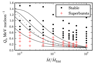
Figure 1.— Mass accretion rate $\dot{M}$ in units of the Eddington-limited rate, $\dot{M}_{\mathrm{Edd}}$, and effective crustal heating parameter, $Q_{\mathrm{b}}$, for 78 models. For each model we indicate whether carbon burning proceeds in a stable manner or as a superburst. The lines correspond to different models for crustal heating (Fig. 18 from Cumming et al. 2006): models with higher neutrino cooling have lower values of $Q_{\mathrm{b}}$ (solid lines); a model with a highly impure crust (dot-dashed line).

We create a series of models for different values of the mass accretion rate and crustal heating. We vary the mass accretion rate in the range where superbursts are observed, $0.01\leq\dot{M}/\dot{M}_{\mathrm{Edd}}\leq 1.00$ (e.g., Keek & in ’t Zand 2008), and we vary the amount of crustal heating between the minimum and maximum values suggested in the literature: $0.1\leq Q_{\mathrm{b}}\leq 1.5$ (e.g., Haensel & Zdunik 2003; Cumming et al. 2006; Gupta et al. 2007). In Fig. 1 we indicate for which values of these parameters the models exhibit superbursts or stable carbon burning. We include the different predictions for $Q_{\mathrm{b}}$ as a function of $\dot{M}$ from Cumming et al. (2006), with the exception of the model that includes Cooper pairs, as its neutrino emissivity was shown to be overestimated (Leinson & Pérez 2006).

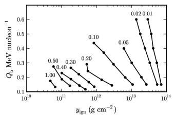
Figure 2.— Superburst ignition column depth $y_{\mathrm{ign}}$ as a function of the crustal heating parameter $Q_{\mathrm{b}}$ for series of models with a fixed mass accretion rate indicated as a fraction of $\dot{M}_{\mathrm{Edd}}$.

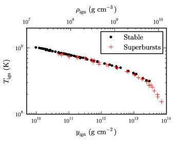
Figure 3.— Ignition (burning) temperature $T_{\mathrm{ign}}$, density $\rho_{\mathrm{ign}}$ and column depth $y_{\mathrm{ign}}$ for models of superbursts (stable carbon burning), in a wide range of mass accretion rates and crustal heating. The relation between $\rho_{\mathrm{ign}}$ and $y_{\mathrm{ign}}$ used here (a power-law fit to the numerical results) is accurate up to $1.2\%$.

Ignition occurs in our models at a column depth of $y_{\mathrm{ign}}\simeq 10^{10}\,\mathrm{g\,cm^{-2}}$ for the models with the highest accretion rate and crustal heating, and at $y_{\mathrm{ign}}\simeq 7\cdot 10^{13}\,\mathrm{g\,cm^{-2}}$ for the coolest models with the lowest accretion rate (Fig. 2, 3). We determine $y_{\mathrm{ign}}$ in our models from the location of the peak temperature just before the start of the runaway (in case of unstable burning), or the peak energy generation rate (in case of steady-state burning), which in both cases identifies the bottom of the carbon-rich layer.

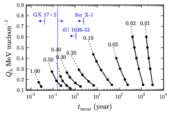
Figure 4.— Superburst recurrence time, $t_{\mathrm{recur}}$, as a function of the crustal heating parameter, $Q_{\mathrm{b}}$, for series of models with a fixed mass accretion rate, indicated as a fraction of $\dot{M}_{\mathrm{Edd}}$. The dotted extrapolations continue after the hottest bursting models to the $Q_{\mathrm{b}}$ value where the first stable model was found in our grid. For three sources we indicate the shortest observed recurrence time (at arbitrary $Q_{\mathrm{b}}$). The average lower limit from BeppoSAX WFC data for nine sources is indicated by a vertical line (Keek et al. 2006).

The bursting models exhibit recurrence times of several days up to thousands of years (Fig. 4). A given recurrence time can be reproduced by a relatively hot model with a certain accretion rate or a colder model with a somewhat higher accretion rate.

3.2. Thermonuclear burning

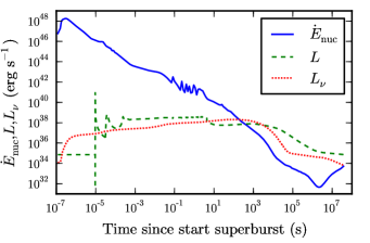
Figure 5.— Energy generation rate, $\dot{E}_{\mathrm{nuc}}$, surface luminosity, $L$, and neutrino luminosity, $L_{\nu}$, as a function of time from the start of one superburst up to the onset of the next, for a model with $\dot{M}=0.30\,\dot{M}_{\mathrm{Edd}}$ and $Q_{\mathrm{b}}=0.13\,\mathrm{MeV\,nucleon^{-1}}$.

To illustrate the thermonuclear burning processes during a superburst we consider a model with $\dot{M}=0.30\,\dot{M}_{\mathrm{Edd}}$ and $Q_{\mathrm{b}}=0.13\,\mathrm{MeV\,nucleon^{-1}}$. The energy generation rate is highest $\sim 2\cdot 10^{-7}\,\mathrm{s}$ after the thermonuclear runaway, and decreases roughly as $t^{-1}$ over the course of $\sim 10^{6}\,\mathrm{s}$ (Fig. 5). Afterwards, the energy generation rate rises again due to increased carbon burning in a newly accreted fuel layer, leading up to the next superburst.

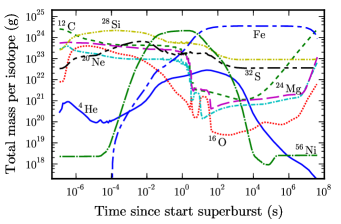
Figure 6.— Total mass for a selection of isotopes as a function of time from the start of one superburst up to the onset of the next, for a model with $\dot{M}=0.30\,\dot{M}_{\mathrm{Edd}}$ and $Q_{\mathrm{b}}=0.13\,\mathrm{MeV\,nucleon^{-1}}$. For Fe the mass at $t=0$ is subtracted: only the produced mass is shown. The Fe mass decreases toward the end because of mass removal at the inner zone of the model (Sect. 2.2), not because of nuclear reactions.

At the superburst onset a large fraction of the available carbon burns through the $\mathrm{{}^{12}C(^{12}C,\alpha)^{20}Ne}$ reaction (Fig. 6). Subsequent $\alpha$-capture reactions produce heavier isotopes, such as $\mathrm{{}^{24}Mg}$, $\mathrm{{}^{28}Si}$, and $\mathrm{{}^{32}S}$. Photodisintegration causes the release of more $\alpha$-particles, whose captures create iron-group elements (e.g., iron and nickel). Electron-captures onto nickel produce iron, which is the most abundant element in the superburst ashes after several seconds. Note that in the employed approximation network the only iron isotope is $\mathrm{{}^{54}Fe}$, whereas calculations with a large network confirm that $\mathrm{{}^{56}Fe}$ is the most abundant isotope.

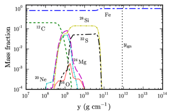
Figure 7.— Mass fraction per isotope as a function of column depth, $y$, approximately $10^{4}\,\mathrm{s}$ after the start of a superburst for a model with $\dot{M}=0.30\,\dot{M}_{\mathrm{Edd}}$ and $Q_{\mathrm{b}}=0.13\,\mathrm{MeV\,nucleon^{-1}}$. The region below $y=10^{7}\,\mathrm{g\,cm^{-2}}$ is omitted, as it has constant carbon and iron fractions. The column depth at which the superburst ignited, $y_{\mathrm{ign}}$, is indicated by the vertical dotted line.

Approximately $10^{4}\,\mathrm{s}$ after the burst start, the total amount of carbon increases again when accretion adds carbon faster than residual burning can take it away (Fig. 6). At this time there is a layer of pure iron directly above the ignition depth, that accounts for over $90\%$ of the mass of the superbursting layer (Fig. 7). This is the composition that forms the outer crust. In the outer part of the envelope, photodisintegration was less efficient due to the lower temperature, resulting in ashes that are more rich in $\mathrm{{}^{20}Ne}$, $\mathrm{{}^{24}Mg}$, $\mathrm{{}^{28}Si}$, and $\mathrm{{}^{32}S}$. The new fuel piles on top of that layer. During the next superburst these isotopes burn to iron group elements. Note that models with stable carbon burning do not undergo photodisintegration, and there the outer crust will be enriched with $\mathrm{{}^{20}Ne}$, $\mathrm{{}^{24}Mg}$, $\mathrm{{}^{28}Si}$, and $\mathrm{{}^{32}S}$.

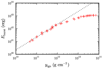
Figure 8.— Ignition column depth, $y_{\mathrm{ign}}$, and the total burst energy, $E_{\mathrm{burst}}$, emitted at the surface for all models. The linear relation below $y_{\mathrm{ign}}\lesssim 10^{12}\,\mathrm{g\,cm^{-2}}$ is indicated by the dotted line.

Part of the generated energy leaves the envelope as photons from the surface, and part is lost in neutrinos (Fig. 5). Neutrino emission is strongest at larger column depths in the substrate. The total burst energy emitted in photons at the surface, $E_{\mathrm{burst}}$, for all bursting models follows a linear relation for ignition below $y_{\mathrm{ign}}\lesssim 10^{12}\,\mathrm{g\,cm^{-2}}$ (Fig. 8). At larger depths $E_{\mathrm{burst}}$ drops below this relation, because an increasing part of the energy is emitted as neutrinos from the substrate (the crust). The maximum $E_{\mathrm{burst}}$ in these models is $1.1\cdot 10^{43}\,\mathrm{erg}$.

3.3. Shock and mixing

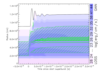
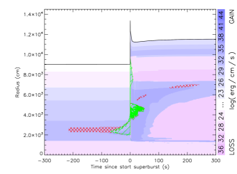
Figure 9.— On three time scales: energy generation/loss (color scale) in the neutron star envelope as a function of time in a short interval around the superburst onset for a model with $\dot{M}=0.30\,\dot{M}_{\mathrm{Edd}}$ and $Q_{\mathrm{b}}=0.13\,\mathrm{MeV\,nucleon^{-1}}$. Green hatching indicates convection, red cross hatching semiconvection.

To study the hydrodynamic processes during a superburst we again consider the model with $\dot{M}=0.30\,\dot{M}_{\mathrm{Edd}}$ and $Q_{\mathrm{b}}=0.13\,\mathrm{MeV\,nucleon^{-1}}$. When the thermonuclear runaway occurs at the bottom of the carbon-rich layer, the burning initially proceeds as a detonation. A combustion wave moves outward, creating a shock. After several microseconds the combustion wave slows down, and burning spreads as a deflagration. The shock continues to travel toward the surface on a microsecond time scale (Fig. 9 top). The top layers are pushed outward, and subsequently fall back on a dynamical time scale of approximately $10^{-5}\,\mathrm{s}$. Afterwards the surface undergoes a damped oscillation. In Fig. 9 we only show the envelope down to $y\simeq 10^{8}\,\mathrm{g\,cm^{-2}}$, which provides the most insight into the dynamic processes (see also Sect. 3.5).

As the outer layers fall back, most of the kinetic energy is dissipated into heat at a depth of $y\simeq 10^{8}$ to $10^{10}\,\mathrm{g\,cm^{-2}}$. Heating by the shock and the fall-back induces some carbon burning in this region, leading to two regions of thermonuclear burning (Fig. 9 top).

Several 100 seconds before and after the superburst onset, convection mixes the composition in the envelope (Fig. 9 middle). Briefly, at the thermonuclear runaway, the convective region reaches close to the surface. After the burst, burning continues at a very low rate at the bottom of the freshly accreted layer (Fig. 9 bottom). During this time no convective mixing takes place. Once the ignition column depth is reached, the next superburst occurs.

The compositional gradient created by the superburst induces thermohaline mixing in the envelope. This mixing is, however, many orders of magnitude slower than that due to convection at the time of burst onset.

3.4. Light curve

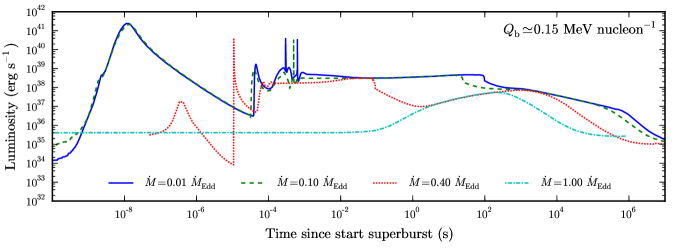
Figure 10.— Light curves of superburst models with $Q_{\mathrm{b}}\simeq 0.15\,\mathrm{MeV\,nucleon^{-1}}$ for a wide range of mass accretion rates.

We generate light curves for all bursting models (Fig. 17). We compare a selection of light curves by taking the coldest model ($Q_{\mathrm{b}}\simeq 0.15\,\mathrm{MeV\,nucleon^{-1}}$) in a wide range mass accretion rates (Fig. 10). The curves consist of several components: a shock breakout peak, a precursor, a transition to the superburst peak, followed by a two-part power law decay. Not every model exhibits each component. After the superburst peak, the decay proceeds as $t^{-0.21}$. Following the break, the decay steepens to $t^{-1.36}$. The models with the lowest mass accretion rates, which are the coldest models with the largest ignition column depth, have the longest decays. The $t^{-0.21}$ power law forms an upper bound to the light curve. Toward higher accretion rates, the time spent in the $t^{-0.21}$ part is smaller, until it becomes absent at the highest rates, and there is a direct transition from the peak to the $t^{-1.36}$ decay.

Whereas the models with lower accretion rate exhibit a precursor, at the highest accretion rates — the hottest models — it is absent. Colder models have longer precursor bursts of up to $\sim 10^{2}\,\mathrm{s}$. We find precursors as short as $\sim 10^{-1}\,\mathrm{s}$. All precursors reach the Eddington limit and cause radius expansion. Depending on the duration of the precursor, the transition to the superburst ‘peak’ around $\sim 10^{3}\,\mathrm{s}$ can exhibit a drop in luminosity below the peak value. The models with longer precursors lack this dip.

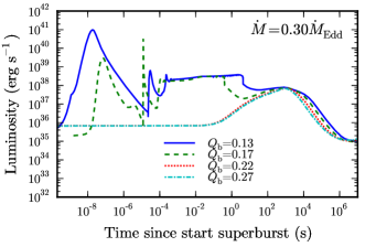
Figure 11.— Light curves of superburst models with $\dot{M}=0.30\,\dot{M}_{\mathrm{Edd}}$ for indicated values of $Q_{\mathrm{b}}$ in units of $\mathrm{MeV\,nucleon^{-1}}$.

To study the effect of crustal heating on the light curve, we compare a series of light curves of simulations with the same mass accretion rate, $\dot{M}=0.30\,\dot{M}_{\mathrm{Edd}}$, but with increasing $Q_{\mathrm{b}}$ (Fig. 11). For increasing $Q_{\mathrm{b}}$, the duration of the superbursts increases from $2.0\cdot 10^{5}\,\mathrm{s}$ to $6.7\cdot 10^{5}\,\mathrm{s}$, and the time spent in the $t^{-0.21}$ phase reduces. The hottest models again lack the precursor. Comparing the models with $Q_{\mathrm{b}}=0.13$ and $Q_{\mathrm{b}}=0.17$, the latter has a shorter duration precursor, as well as a deeper dip in the light curve between the precursor and the main peak after 1000 s.

Some light curves show a shorter precursor phase than expected, exhibiting instead a small bump immediately after the precursor (e.g., some models with $\dot{M}=0.10\,\dot{M}_{\mathrm{Edd}}$ in Fig. 17). This is due to the relaxation of the outer atmosphere following the end of the radius expansion phase, and may be attributed to poor resolution at the surface of the models. It is not caused by burning or mixing processes.

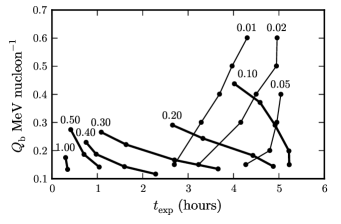
Figure 12.— Exponential decay time, $t_{\mathrm{exp}}$, vs. crustal heating, $Q_{\mathrm{b}}$, for series of models with a certain mass accretion rate, indicated as a fraction of $\dot{M}_{\mathrm{Edd}}$.

We define the exponential decay time, $t_{\mathrm{exp}}$, of our light curves as the time it takes from the superburst peak around $t=10^{3}\,\mathrm{s}$ to drop one e-fold in luminosity (Fig. 12). It ranges from 18 minutes to 5.2 hours.

3.5. Precursor burst

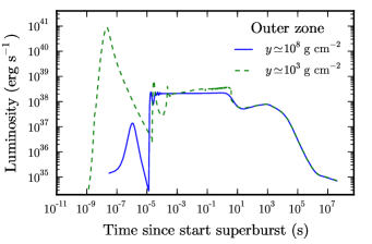
Figure 13.— Light curves of superburst models with $\dot{M}=0.30\,\dot{M}_{\mathrm{Edd}}$ and $Q_{\mathrm{b}}=0.13\,\mathrm{MeV\,nucleon^{-1}}$ with different column depths for the outer zone.

As noted by Weinberg & Bildsten (2007), the overpressure of the shock is larger at lower column depths. Hence, at lower column depths the shock induces more heating and a larger radius expansion. To illustrate this, we compare the light curves of two models that have both $\dot{M}=0.30\,\dot{M}_{\mathrm{Edd}}$ and $Q_{\mathrm{b}}=0.13\,\mathrm{MeV\,nucleon^{-1}}$, but one model extends to a column depth of $y\simeq 10^{8}\,\mathrm{g\,cm^{-2}}$, and the other to $y\simeq 10^{3}\,\mathrm{g\,cm^{-2}}$ (Fig. 13). The model with the more extended envelope has a shock breakout peak that has an approximately 50 times faster rise and a super-Eddington luminosity of $0.89\cdot 10^{41}\,\mathrm{erg\,s^{-1}}$, whereas the other model’s shock peak reaches only $1.4\cdot 10^{37}\,\mathrm{erg\,s^{-1}}$. After the shock breakout, the model with the more extended envelope has stronger radius expansion and larger variations in luminosity. The latter reaches a $1.7$ times higher value than for the other model. The stronger shock heating leads to a lower opacity, which increases the Eddington limit, allowing for higher surface luminosities. 4 seconds after the start of the superburst, the radius expansion phase ends. The more extended atmosphere model displays a sharper drop in luminosity. The smoother luminosity decrease of the other model may lead to the interpretation that the precursor in this case has a duration that is several seconds shorter. After the precursor, the light curves of the two models are virtually identical. Therefore, both the duration and the peak luminosity of the shock breakout and the precursor depend greatly on the extend of the atmosphere. Note that the neutron star photosphere is expected at a column depth of approximately $y\simeq 1\,\mathrm{g\,cm^{-2}}$, and it is likely that at that column depth the shock breakout peak as well as the precursor properties are different from our results.

The shock heating of the outer layers induces some carbon burning, but the amount of heat generated by the nuclear reactions is too small to substantially alter the light curve, as we checked by comparing to a model where burning was disabled in that region. Therefore, the precursor is in these models virtually completely powered by shock heating.

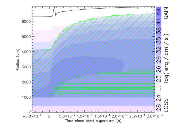
Figure 14.— For a model without a precursor ($\dot{M}=0.30\,\dot{M}_{\mathrm{Edd}}$ and $Q_{\mathrm{b}}=0.22\,\mathrm{MeV\,nucleon^{-1}}$) the energy generation/loss (color scale) in the neutron star envelope as a function of time in a short interval around the superburst onset. Green hatching indicates convection.

The hottest models at the highest accretion rates do not show precursors at all (Sect. 3.4). We compare the model with a precursor from Fig. 9 to a hotter one ($Q_{\mathrm{b}}=0.22\,\mathrm{MeV\,nucleon^{-1}}$) that lacks a precursor (Fig. 14). The hotter model’s burst has a shallower ignition depth, and is, consequently, less powerful. The shock causes only minimal radius expansion, and does not provide enough heating to produce a precursor burst or to ignite carbon close to the surface. In this case there is only one region of carbon burning (Fig. 14).

3.6. Comparison to 4U 1636-53

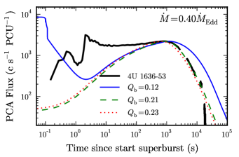
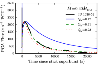
Figure 15.— Comparison of the observed light curve of 4U 1636-53 to light curves of superburst models with $\dot{M}=0.10\,\dot{M}_{\mathrm{Edd}}$ and $\dot{M}=0.40\,\dot{M}_{\mathrm{Edd}}$ for indicated values of $Q_{\mathrm{b}}$ on a logarithmic scale. The bottom figure shows the data of the middle one on a linear scale.

We compare several of our simulated light curves to the observed light curve from the superburst of 4U 1636-53 (catalog ), that was observed with the Proportional Counter Array (PCA) on-board the Rossi X-ray Timing Explorer (RXTE) (Fig. 15; Strohmayer & Markwardt 2002; see also Kuulkers 2004; Kuulkers et al. 2004). The PCA consists of five Proportional Counter Units (PCUs). We use standard 1 data from PCU 2 in the full instrument band-pass, and correct it for dead time following the prescription from the RXTE Cookbook. We subtract the persistent emission as measured from the end of the last orbit that we consider. In this we assume the persistent flux to remain constant during the superburst, which is probably not the case: in the day preceding the superburst, the persistent flux varied by around $10^{2}\,\mathrm{counts\,s^{-1}\,PCU^{-1}}$. Because the superburst lasts longer than the orbit of RXTE, the observation was interrupted three times by Earth occultations, resulting in gaps in the light curve.

The simulated light curves are constructed taking into account the PCA’s instrument response and astrophysical effects. We use the surface radius and temperature from our models to calculate the blackbody emission from the superbursts. The temperature is increased by a typical color correction factor of $1.5$ to account for deviation from a pure blackbody spectrum due to Compton scattering close to the neutron star surface (e.g., Suleimanov et al. 2011). We apply a gravitational redshift of $1+z=1.26$ for a neutron star with a gravitational mass of $1.4\,M_{\odot}$ and a radius of $11.2\,\mathrm{km}$ in the local rest frame (see Sect. 2.5; Appendix B). The effect of interstellar absorption by hydrogen is taken into account using the model by Morrison & McCammon (1983), that uses solar abundances from Anders & Ebihara (1982), using a hydrogen column of $2.5\cdot 10^{21}\,\mathrm{cm^{-2}}$ (Asai et al. 2000). We take into account the effective area of the PCUs at different energies using the table provided with the software package PIMMS version 4.2. The curves are scaled such that the superburst peak fluxes match at $t\simeq 800\,\mathrm{s}$.

We obtain a measure of the persistent luminosity during the month preceding and following the superburst from flux measurements obtained with the PCA on RXTE and the Wide-Field Cameras (WFCs) on-board BeppoSAX, that are collected in the Multi-Instrument Burst Archive (MINBAR; e.g., Keek et al. 2010). A bolometric correction is available for several orbits. We use the mean value: $1.4$. By comparing to the Eddington luminosity for a $1.4\,M_{\odot}$ neutron star with a $11.2$ km radius and an atmosphere of solar composition (Sect. 2.7), we find that the accretion rate was $0.12\,\dot{M}_{\mathrm{Edd}}$ with a root mean-squared deviation of $10\%$.

For models with an accretion rate of $0.10\,\dot{M}_{\mathrm{Edd}}$, the scaling factor for our simulated curves is approximately $0.42$. This factor can be explained by a $54\%$ larger distance to the source than the $6\,\mathrm{kpc}$ that we assumed (Galloway et al. 2008). These models predict a much longer decay time than observed (Fig. 15). The best fit is provided by a model at higher accretion rate: $Q_{\mathrm{b}}=0.21\,\mathrm{MeV\,nucleon^{-1}}$ and $\dot{M}=0.40\,\dot{M}_{\mathrm{Edd}}$. For those models the scaling factor is approximately $0.63$, which can be explained by a $26\%$ larger distance to the source. The best fit model lacks a precursor burst.

4. Discussion

4.1. Superburst models

We create $86$ models of a neutron star envelope with accretion of carbon-rich material in the range of observed accretion rates, assuming a range of values for the crustal heating parameter $Q_{\mathrm{b}}$ (Fig. 1). We follow the thermonuclear burning of the accreted carbon, which proceeds as flashes (superbursts) in some cases, whereas at higher values of $Q_{\mathrm{b}}$ burning becomes stable. We compare the amount of crustal heating of our bursting models to models of $Q_{\mathrm{b}}$ as a function of $\dot{M}$ (Cumming et al. 2006). Only the lowest curve that spans the entire range of mass accretion rates lies within the range of $Q_{\mathrm{b}}$ where we find unstable carbon burning. This implies that a high neutrino emissivity of the neutron star core is favored.

Note that superbursting sources mostly accrete hydrogen or helium-rich material, which create carbon-rich ashes from thermonuclear burning. By directly accreting the latter composition, we skip the computationally expensive hydrogen/helium burning, making it possible to simulate the long superburst recurrence times. Hydrogen/helium burning may increase the temperature of the envelope, which can be modelled by an extra contribution to $Q_{\mathrm{b}}$.

Carbon ignition occurs in our models at a column depth $y_{\mathrm{ign}}$ between approximately $10^{10}\,\mathrm{g\,cm^{-2}}$ and $10^{14}\,\mathrm{g\,cm^{-2}}$ (Fig. 2; Fig. 3). The stable burning models extend to lower $y_{\mathrm{ign}}$ than the bursting models, because at a given accretion rate stable burning requires a higher crustal heat flux than unstable burning, which leads to shallower ignition.

In the relation between the ignition depth (or density) and temperature (Fig. 3), there is a down turn in the trend for $y_{\mathrm{ign}}\gtrsim 10^{13}\,\mathrm{g\,cm^{-2}}$, which is due to increased screening of the Coulomb barrier of the carbon ions at temperatures below $T\lesssim 3\cdot 10^{8}\,\mathrm{K}$ and densities in excess of $\rho\gtrsim 10^{9}\,\mathrm{g\,cm^{-3}}$ (Salpeter & van Horn 1969; Yakovlev et al. 2006; see also, e.g., Brown & Bildsten 1998). This is the transition from thermonuclear burning to pycnonuclear burning, which sets in at temperatures $T\lesssim 10^{8}\,\mathrm{K}$. The ignition conditions are more uncertain in this regime, because the possible formation of a crystal lattice may require higher densities for carbon fusion (Yakovlev et al. 2006).

When the ignition column depth exceeds $y_{\mathrm{ign}}\gtrsim 4\cdot 10^{11}\,\mathrm{g\,cm^{-2}}$ we find superbursts to be powerful enough to drive a shock to the surface (see also Weinberg et al. 2006; Weinberg & Bildsten 2007). At the start of the thermonuclear runaway, the burning time scale at the ignition depth becomes shorter than the dynamical time scale. A combustion wave moves outward, depleting the inner zones of carbon, while initiating a shock. This detonation phase lasts only a few microseconds, until the velocity of the combustion wave is sufficiently reduced, and burning continues to spread as a deflagration. The shock then no longer follows the burning front, but speeds ahead toward the surface.

4.2. Decay profile

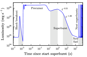
Figure 16.— Light curve of the model with $\dot{M}=0.30\,\dot{M}_{\mathrm{Edd}}$ and $Q_{\mathrm{b}}=0.13\,\mathrm{MeV\,nucleon^{-1}}$ , where the outer zone is at a column depth of $\sim 10^{8}\,\mathrm{g\,cm^{-2}}$. We indicate the different phases of the superburst. Several followup superbursts are shown.

The superburst light curves consist of a shock breakout, a precursor, a rise to the ‘superburst peak’, and two power-law decay phases with $L\propto t^{-0.21}$ and $L\propto t^{-1.36}$ (Fig. 16). These power law indices are consistent with the results obtained by Cumming et al. (2006) and by Weinberg & Bildsten (2007). Cumming & Macbeth (2004) explain that the first power law component is due to radiative cooling when a cooling wave propagates from the surface inwards (see also Cumming et al. 2006). Once this wave reaches the bottom of the carbon burning layer, the cooling transitions to the steeper power law. Hotter models with high accretion rates burn shallower columns, such that the $L\propto t^{-0.21}$ phase lasts shorter in these models. For models with the highest values for $\dot{M}$ and $Q_{\mathrm{b}}$, this phase is absent in the light curve. After the superburst peak an immediate transition is made to $L\propto t^{-1.36}$.

The $L\propto t^{-1.36}$ ends when burning of newly accreted carbon starts dominating the light curve, up to the thermonuclear runaway of the next superburst (Fig. 16).

Observationally, the duration of the decay is often measured by fitting an exponential to the light curve. Even though theoretically we expect the decay to follow a power law, the quality of the data is often such that an exponential still provides a good fit. Decay times have been observed between $0.7$ and $6.0$ hours (e.g., Keek & in ’t Zand 2008). We determine the exponential decay time $t_{\mathrm{exp}}$ for our light curves as the time it takes for the luminosity to drop from the peak by one e-fold (Fig. 12). If this time falls within the $L\propto t^{-0.21}$ phase, where all models share the same curve, $t_{\mathrm{exp}}$ is mainly dependent on the peak luminosity: a higher peak means $\mathrm{e}^{-1}L_{\mathrm{peak}}$ is reached earlier on the $L\propto t^{-0.21}$ curve. This yields smaller values of $t_{\mathrm{exp}}$ for colder models, because they have larger peak luminosities. If $t_{\mathrm{exp}}$ reaches into the $L\propto t^{-1.36}$ phase, $t_{\mathrm{exp}}$ depends less on the peak, and more on the actual decay of the light curve. Colder models with lower accretion rates have longer $t_{\mathrm{exp}}$ in this case. The difference in behavior during the two power law decay phases makes it difficult to use the published observed $t_{\mathrm{exp}}$ to constrain model parameters. It is, therefore, more instructive to fit a two-component power law decay, if the data quality allows for it (Cumming et al. 2006; Keek et al. 2008; Kuulkers et al. 2010; Fig. 15).

4.3. Precursor bursts

At the start of the thermonuclear runaway a shock travels from the ignition depth to the surface. The shock breakout is visible in the light curve as a short bright peak in the light curve, when during a fraction of a microsecond super-Eddington luminosities are reached (e.g., Fig. 13). The atmosphere is pushed upwards, before it falls back on a dynamical time scale of the order of $10^{-5}\,\mathrm{s}$, and undergoes damped oscillations. The shock and the fall-back deposit heat for the different models at column depths between $y\simeq 10^{8}\,\mathrm{g\,cm^{-2}}$ and $y\simeq 10^{10}\,\mathrm{g\,cm^{-2}}$. The cooling of these layers on thermal time scales of up to approximately $10^{2}\,\mathrm{s}$ is visible as a precursor burst. We find that the peak luminosity of the shock breakout and the amplitude of the oscillations depends strongly on the resolution of the atmosphere in the models. The shock over-pressure is greater closer to the surface (Weinberg & Bildsten 2007), where the density is lower, causing a stronger shock breakout. Note that not all models produce a precursor: superbursts with $y_{\mathrm{ign}}\lesssim 4\cdot 10^{11}\,\mathrm{g\,cm^{-2}}$ are not powerful enough to drive a shock. These models still reach a temperature of $T\simeq 5\cdot 10^{8}\,\mathrm{K}$ at a column depth of $y=10^{8}\,\mathrm{g\,cm^{-2}}$. This is too cold for carbon burning, but it is hot enough to trigger the thermonuclear runaway of helium burning (e.g., Bildsten 1998), leading to a short hydrogen/helium precursor burst.

Our models confirm the scenario of precursors due to shock heating (Weinberg & Bildsten 2007). Weinberg & Bildsten (2007) created models of superbursts in a neutron star with a helium-rich envelope. They found that without the helium, carbon burning at lower depths produces a weak precursor. In contrast, we find that the shock heating is much stronger than any carbon burning at this depth, resulting in a bright precursor from heating alone. Their light curves exhibit a precursor that starts several seconds after the shock breakout. The shock leaves a the outer envelope isothermal, delaying the precursor emission by a thermal time scale. Weinberg & Bildsten (2007) describe that at this point in the simulation they assume a new hydrostatic equilibrium in the outer layers. Instead, we perform a fully self-consistent calculation that includes the fall-back of the outer layers, which disrupts the flat temperature profile, and causes the light curve to change much faster on a dynamical time scale. Furthermore, most of the energy of the shock went into the expansion of the outer layers, and is only converted into heat during the fall-back. This generates, therefore, not only a precursor more quickly on a dynamical time scale, but also a much more powerful precursor burst that can last up to $10^{2}\,\mathrm{s}$.

The light travel time around a neutron star with a $10\,\mathrm{km}$ radius is $1.1\cdot 10^{-4}\,\mathrm{s}$. Therefore, assuming instantaneous ignition throughout the entire envelope, any detail in the light curve at shorter times, such as the shock breakout and the subsequent oscillations, will be smeared out.

Only for seven superbursts the onset has been observed. Three times a precursor burst was seen directly at the start of the superburst (Strohmayer & Brown 2002; Strohmayer & Markwardt 2002; in ’t Zand et al. 2003). For two superburst candidates from GX 17+2 the onset was seen, but because of the quality of the data only hints of precursors were observed (in ’t Zand et al. 2004). The tentative observation of the superburst rise from 4U 1608-522 with HETE-2 did not exhibit a precursor. The data quality allows for only a weak precursor.

The precursors of 4U 1636-53 and 4U 1254- 69 have a higher peak flux than the superburst. For 4U 1820-30 the superburst itself was exceptionally bright, and the precursor’s peak flux was approximately $15\%$ lower. The light curves of the precursor bursts exhibit a double peak, similar to photospheric radius expansion (PRE) bursts. For none of these bursts, however, is spectroscopic information available at sufficient time resolution or of sufficient quality to confirm the PRE nature of these bursts. Nonetheless, the precursor bursts in our models all reach the Eddington limit, resulting in PRE.

There is a tentative observation of the onset of the superburst from 4U 1608-522 with the WXM and FREGATE instruments on-board the HETE-2 satellite (Keek et al. 2008). At the end of an orbit there is an increase in the count rate visible for $50\,\mathrm{s}$. No short precursor can be discerned. The superburst occurred during a transient outburst, when the accretion rate exceeded $0.10\,\dot{M}_{\mathrm{Edd}}$. The time-averaged rate in the years before the superburst, however, was only $0.01\,\dot{M}_{\mathrm{Edd}}$. Our models at low accretion rates include precursors with durations in excess of $50\,\mathrm{s}$. This suggests the possibility that the entire flare observed with HETE-2 was part of the precursor.

Kuulkers et al. (2002) refer to a burst from KS 1731-260, that occurred $200\,$s before the superburst rise, as precursor. The $200\,\mathrm{s}$ is much shorter than the typical burst recurrence time for this source of several hours, as well as shorter than the superburst duration. The three other precursors, however, occurred immediately prior to the rise of the superburst. Also, this burst was relatively weak compared to most other bursts from this source, but several bursts with a similar peak flux have been observed. Therefore, we suggest that the burst preceding the superburst of KS 1731-260 is an ordinary burst that by chance was close to the superburst. Perhaps heating from the stable carbon burning before the superburst thermonuclear runaway caused the normal burst to ignite earlier, resulting in a relatively weak burst.

4.4. Burning ashes and crustal composition

Carbon burning and subsequent $\alpha$-capture reactions create $\mathrm{{}^{20}Ne}$, $\mathrm{{}^{24}Mg}$, $\mathrm{{}^{28}Si}$, and $\mathrm{{}^{32}S}$ (e.g., Schatz et al. 2003a). For stable burning models these isotopes combined with ⁵⁶Fe from the ashes of hydrogen/helium bursts (our accretion composition; e.g., Woosley et al. 2004) form the composition of the outer crust. In superbursting models, photodisintegration provides more $\alpha$-particles for captures, creating iron group elements (Fig. 6). Therefore, superbursting neutron stars have an outer crust composed of mostly iron.

In the bursting models there is a region at a depth lower than the ignition column depth, where the temperature is insufficient for photodisintegration. Therefore, carbon burning in this layer creates $\mathrm{{}^{20}Ne}$, $\mathrm{{}^{24}Mg}$, $\mathrm{{}^{28}Si}$, and $\mathrm{{}^{32}S}$ (Fig. 7). Note that the most abundant element is iron from the accretion composition. The next superburst ignites on top of this layer, and these isotopes burn to iron. A layer enriched in $\mathrm{{}^{20}Ne}$, $\mathrm{{}^{24}Mg}$, $\mathrm{{}^{28}Si}$, and $\mathrm{{}^{32}S}$ in principle has a somewhat lower opacity than a pure iron layer, resulting in a larger ignition column depth $y_{\mathrm{ign}}$. The layer composition is, however, dominated by iron, which limits the changes in opacity. We do not find a difference between $y_{\mathrm{ign}}$ of the first superburst in a series and subsequent bursts that can be attributed to such a compositional inertia effect (cf. Woosley et al. 2004).

4.5. Recurrence times

The bursting models exhibit recurrence times of several days up to thousands of years (Fig. 4). We compare these to the three cases where more than one superburst has been observed from the same source. For these sources we derive the time averaged mass accretion rate from the persistent X-ray luminosity as reported in the MINBAR catalog (e.g., Keek et al. 2010), expressed in units of the Eddington limited rate for our choice of neutron star parameters (Sect. 2.7). The typical uncertainty in measurements of the accretion rate are several tens of percents. Due to the presence of frequent data gaps, the observed recurrence times have to be regarded as upper limits (e.g., Keek et al. 2010 for the case of bursts with short recurrence times).

Ser X-1 has a mean mass accretion rate of $0.31\,\dot{M}_{\mathrm{Edd}}$, and superbursts observed at least 2.4 years apart (Cornelisse et al. 2000; Kuulkers 2009). The models with $0.30\,\dot{M}_{\mathrm{Edd}}$ have a maximum recurrence time of $t_{\mathrm{recur}}=1.7\,\mathrm{years}$ ($2.1$ years for a gravitational redshift of $z+1=1.26$), whereas models with $0.20\,\dot{M}_{\mathrm{Edd}}$ reproduce the observed $t_{\mathrm{recur}}$. Therefore, the accretion rate is somewhat lower than observationally inferred, or the actual $t_{\mathrm{recur}}$ of this source is shorter than the upper limit.

Four superbursts have been observed from GX 17+2; two only 15 days apart (in ’t Zand et al. 2004). The mass accretion rate is unusually high for a bursting source: on average $1.21\,\dot{M}_{\mathrm{Edd}}$. The models with a mass accretion rate of $1.00\,\dot{M}_{\mathrm{Edd}}$ exhibit recurrence times up to 11 days (13 days for $z+1=1.26$). It is likely that models with a smaller accretion rate of $\sim 0.9\,\dot{M}_{\mathrm{Edd}}$ will produce the observed recurrence time. This rate is within the uncertainty of the observed accretion rate.

The shortest time interval between two observed superbursts of 4U 1636-53 is 1.1 year (Wijnands 2001; Strohmayer & Markwardt 2002; Kuulkers et al. 2004; Kuulkers 2009). The time averaged mass accretion rate of 4U 1636-53 is $0.12\,\dot{M}_{\mathrm{Edd}}$, but the models close to this rate produce a recurrence time of at least $7\,\mathrm{years}$ ($9$ years for $z+1=1.26$). Part of this problem may be explained by the uncertainties in the measured mass accretion rate of several tens of percents. Other explanations for this discrepancy may be found in our assumptions for the carbon mass fraction and of the effective gravity in the neutron star envelope.

For nine sources, most of which with accretion rates close to $0.10\,\dot{M}_{\mathrm{Edd}}$, a lower limit to the superburst recurrence time was derived from the BeppoSAX Wide-Field Camera (WFC) data (Keek et al. 2006). The average lower limit of $60$ days is indicated in Fig. 4, and is consistent with the model results for the sources with mass accretion rates up to $0.5\,\dot{M}_{\mathrm{Edd}}$.

The same recurrence time can be reproduced by models with a mass accretion rate that varies by several tens of percents, and different values of $Q_{\mathrm{b}}$. This spread in mass accretion rate is of the order of the uncertainty in the observed rate, which makes it difficult to constrain $Q_{\mathrm{b}}$ from the observed recurrence times.

4.6. Comparison to 4U 1636-53

The most detailed superburst light curves have been observed with the PCA on RXTE: one from 4U 1636-53 (Strohmayer & Markwardt 2002) and one from 4U 1820-30 (Strohmayer & Brown 2002). The latter source is an ultra-compact binary system, which implies that the accreted material is hydrogen-deficient. The material that burns in the superburst is thought to be more carbon-rich than the composition that we assumed in our calculations. Its superburst is atypical, as the superburst peak reached the Eddington limit and exhibited radius expansion. For these reasons we do not compare to this source, and focus our attention on the superburst from 4U 1636-53.

The superburst from this source started with a short precursor that showed behavior consistent with photospheric radius expansion, and that decayed on a 10 s time scale. The superburst decay was observable for $5.5\,\mathrm{hours}$. The average mass accretion rate of this source over the past decade is $0.12\,\dot{M}_{\mathrm{Edd}}$ (Sect. 4.5). The models close to this rate exhibit a much longer decay time scale, even for high crustal heating (Fig. 15 top). Also, the precursors of these models last longer than observed. The decay is best fit by a model with a four times higher accretion rate of $\dot{M}=0.40\,\dot{M}_{\mathrm{Edd}}$ and with $Q_{\mathrm{b}}=0.21\,\mathrm{MeV\,nucleon^{-1}}$ (Fig. 15 middle). This models, however, does not have a precursor, and the part leading up to the superburst peak is not well reproduced. This may be due to the fact that the atmosphere of 4U 1636-53’s neutron star is probably hydrogen-rich, instead of carbon-rich as we assumed. While our modeled burst is not powerful enough to heat the atmosphere by a shock, the temperature in the atmosphere is high enough, $T\simeq 6\cdot 10^{8}\,\mathrm{K}$, to ignite a hydrogen/helium precursor burst.

If we were to assume that $\dot{M}=0.40\,\dot{M}_{\mathrm{Edd}}$ is a good approximation, Fig. 15 (bottom) illustrates how sensitive the decay depends on the crustal heating parameter $Q_{\mathrm{b}}$.

The discrepancy between the observed light curve and the models at $0.10\,\dot{M}_{\mathrm{Edd}}$ adds to the problem we noted earlier that the recurrence times predicted by the models with $0.10\,\dot{M}_{\mathrm{Edd}}$ are substantially longer than the observational upper limit (Fig. 4). The answer to this problem may lie in the fact that we only considered one carbon fraction for the envelope, and one value for the effective gravity. Variations of these parameters could yield the shallower ignition implied by our models. Another possibility are multi-dimensional effects that we cannot model in our one-dimensional code. Pulsations at the spin frequency of the neutron star were observed during $800\,\mathrm{s}$ close to the superburst peak (Strohmayer & Markwardt 2002). This indicates that the emission was anisotropic during a quite long period after superburst ignition, which hints at the presence of multi-dimensional effects.

5. Conclusions

To study carbon flashes (superbursts), we constructed 86 one-dimensional multi-zone models of the envelope of a neutron star that accretes carbon-rich material, for different mass accretion rates and amounts of crustal heating. These are the first such models that were constructed by following the accumulation of the fuel layer and the thermonuclear burning of carbon during a series of superbursts. The stability of carbon burning is investigated as a function of the amount of crustal heating. We reproduced the two-component power-law decay (Cumming & Macbeth 2004). Not all models, however, exhibit the first component: the hotter models at higher mass accretion rates show a direct transition from the superburst peak to the second (steeper) power-law component.

The superburst ashes that form the outer crust are primarily composed of iron. Carbon burning higher up in the envelope produces isotopes with mass numbers around $30$. The next superburst ignites in this layer. We do not find a compositional inertia effect, as seen for hydrogen/helium bursts (Woosley et al. 2004), because the layer composition is dominated by the accreted fraction of iron. In case of a larger carbon fraction of the fuel layer, however, such an effect may become important.

We obtain a precursor burst due to shock heating, similar to Weinberg & Bildsten (2007). We find that heating by the shock and the fall-back of expanded layers is sufficient for a strong precursor, that starts approximately $10^{-5}\,\mathrm{s}$ after the shock breakout, instead of seconds. For hot models, at large accretion rates, the superburst is not powerfull enough to generate a shock and thus a precursor from shock heating. At low accretion rates the precursors have durations as long as $10^{2}\,\mathrm{s}$. This may explain the lack of a short precursor in the observation of the onset of the superburst from 4U 1608-522.

Comparing the model light curves to the superburst observations with the PCA on RXTE of 4U 1636-53, the models at the observationally inferred mass accretion rate overpredict the superburst duration and the recurrence time. The best agreement is found with models at a three times higher accretion rate. The discrepancy may be caused by the values we assumed for the carbon fraction in the ocean and the effective gravity. This can be studied further with one-dimensional models. Alternatively, it can be a sign of multi-dimensional effects, where a higher local accretion rate is responsible the observed behavior.

We studied the dependence of observables, such as the recurrence time and the shape of the light curve, on the amount of crustal heating $Q_{\mathrm{b}}$. While we show that these observables can depend strongly on $Q_{\mathrm{b}}$, the example of 4U 1636-53 indicates that without a good agreement of the behavior as a function of mass accretion rate, it is difficult to constrain $Q_{\mathrm{b}}$.

Appendix A Model light curves

We present all light curves resulting from the models indicated in Fig. 1 (Fig. 17). The curves do not contain corrections for the gravitational redshift near neutron stars. See Section 3.4 for further details.

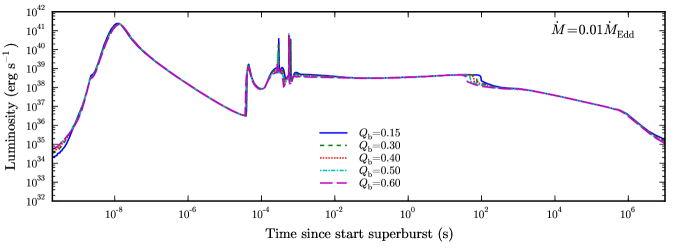
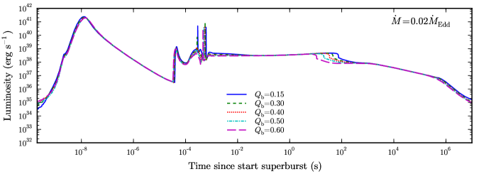
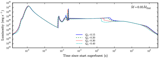
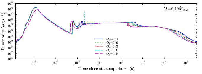
Figure 17.— Model light curves. Each panel shows the light curves resulting from models with a certain mass accretion rate $\dot{M}$, at different values of the crustal heating parameter $Q_{\mathrm{b}}$. Continued on next page.

Fig. 17 continued Continued on next page.

Fig. 17 continued

Appendix B General relativistic corrections

B.1. Introduction

The thin surface layer of a neutron star in which the X-ray burst occurs can locally be treated in Newtonian physics for $\Delta r\ll r$, where $r$ is the radius of the star and $\Delta r$ is the thickness of the surface layer. For neutron stars general relativistic (GR) effects are important, but the Kepler code, which is employed in this study, uses Newtonian gravity. Therefore, we need to correct for GR effects to allow for proper interpretation and comparison with observations. This comprises two types of corrections: first, identifying the neutron star masses and radii that give same relativistic gravitational acceleration as the Newtonian acceleration that was used from the input mass and radius. Second, correct the results for time dilatation (of the light curve and decrease of the accretion rate; $\sim(1+z)$, where $z$ is the gravitational redshift) and weakening of luminosity ($\sim(1+z)^{2}$).

B.2. Translating Newtonian to GR

When only Newtonian gravity is used in the calculation, neglecting the strengthening of gravity by a factor $(1+z)$, the result can still be interpreted as that of a star with a different mass, ${M_{\mathrm{1}}}$, and radius, ${r_{\mathrm{1}}}$, and correspondingly adjusted (smaller) redshift, ${z_{\mathrm{1}}}$, such that the GR acceleration equals the Newtion acceleration in the calculation. Below the scaling laws for interpreting mass and radius are derived.

Thorne (1977) gives the volume redshift factor

$$\mathcal{V}=1\left/\sqrt{1-2GM/(c^{2}r)}\right.,$$ (B1)

which will be called $1+z$ here. Relativistic gravitational acceleration is given by (e.g., Woodhouse 2007)

$${g_{\mathrm{rel}}}=-(1+z)GM\left/r^{2}\right.=GM\left/\left(r^{2}\sqrt{1-2GM/(c^{2}r)}\right)\right..$$ (B2)

We now define a radius ${r_{\mathrm{1}}}$ and an actual gravitational mass, ${M_{\mathrm{1}}}$, such that the GR gravity at this point equals the Newtonian gravity, $g$, at radius $r$, i.e., ${g_{\mathrm{rel,1}}}\stackrel{{\scriptstyle!}}{{=}}g$:

$$GM\left/r^{2}\right.\stackrel{{\scriptstyle!}}{{=}}G{M_{\mathrm{1}}}\left/\left({r_{\mathrm{1}}}^{2}\sqrt{1-2G{M_{\mathrm{1}}}\left/\left(c^{2}{r_{\mathrm{1}}}\right)\right.}\right)\right.\;.$$ (B3)

This can be rewritten as

$$\varphi^{2}+2\varphi\zeta\xi^{3}-\xi^{4}=0\qquad\mbox{with}\qquad\xi={r_{\mathrm{1}}}/r\;,\qquad\varphi={M_{\mathrm{1}}}/M\;,\qquad\zeta=GM\left/\left(c^{2}r\right)\right.\;,$$ (B4)

where $\zeta$ is the gravitational radius of the original problem.

B.2.1 Given Mass

Assuming a mass ${M_{\mathrm{1}}}=\varphi M$, the physical solution of this 4^th order equation for $\xi$ is given by

$$\xi=\frac{\zeta\,\varphi}{2}\left(1+\sqrt{1-A}+\sqrt{2+A+2/\sqrt{1-A}}\right)$$

$$A=\sqrt[3]{2/9}\left(B^{2}/\varphi^{2}-2\sqrt[3]{6}\right)\left/\left(B\zeta^{2}\right)\right.\;,\qquad B=\sqrt[3]{9\,\zeta^{2}\,\varphi^{4}+{\sqrt{3}}\,\varphi^{3}\,{\sqrt{16+27\,\zeta^{4}\,\varphi^{2}}}}\;.$$ (B5)

The radius ${r_{\mathrm{1}}}$ at which the GR gravitational acceleration matches the Newtonian one for the assumed radius, $r$, is thus given by ${r_{\mathrm{1}}}=\xi r$. The redshift factor ${z_{\mathrm{1}}}$ for radius ${r_{\mathrm{1}}}$ and mass ${M_{\mathrm{1}}}$ is given by

$$1+{z_{\mathrm{1}}}=1\left/\sqrt{1-2G{M_{\mathrm{1}}}/(c^{2}{r_{\mathrm{1}}})}\right.=1\left/\sqrt{1-2\zeta\varphi/\xi}\right.\;.$$ (B6)

Using Equation (B3) one obtains

$$\xi^{2}/\varphi=1+{z_{\mathrm{1}}}\;.$$ (B7)

Using these relations , the light curve for an observer at infinity has to be time dilated by $1+{z_{\mathrm{1}}}$. Due to the larger radius, the surface area is increased by $\xi^{2}=\varphi(1+{z_{\mathrm{1}}})$ and thus luminosity has to be scaled by $\xi^{2}/(1+{z_{\mathrm{1}}})^{2}$, i.e., decreased by a factor $(1+{z_{\mathrm{1}}})/\varphi$. Similarly, the apparent accretion rate for an observer at infinity scales as $\xi^{2}/(1+{z_{\mathrm{1}}})=\varphi$, that is, does not need to be modified if $M={M_{\mathrm{1}}}$. For a NS with $1.4\,{M_{\odot}}$ (gravitational) mass and 10 km Newtonian model radius and assuming $M={M_{\mathrm{1}}}$, i.e., $\varphi=1$, $\zeta=0.206666$, one obtains $\xi=1.12176$ and ${z_{\mathrm{1}}}=0.25835$.

B.2.2 Given Radius

On the other hand, if we know the true radius, ${r_{\mathrm{1}}}=\xi r$, we can determine the mass corresponding to the gravity we used by solving Eq. (B4) for $\varphi$ and then use Eq. (B6) or (B7) to determine ${z_{\mathrm{1}}}+1$,

$$\varphi={M_{\mathrm{1}}}/M=\zeta\xi^{3}\left(\sqrt{1+1\left/\left(\xi^{2}\zeta^{2}\right)\right.}-1\right)\;.$$ (B8)

For our parameters we then obtain $\xi=1$, $\varphi=0.81440$, i.e., ${M_{\mathrm{1}}}=1.1401630\,{M_{\odot}}$, ${z_{\mathrm{1}}}=0.22789465$.

B.2.3 Minimal Adjustment

Alternatively, we could search for a minimum deviation of both $\varphi$ and $\xi$ from $1$, that is, setting $\xi=1/\varphi$ in Eq. (B4):

$$\varphi^{6}+2\zeta\varphi^{2}-1=0$$ (B9)

with the physical solution

$$\varphi^{2}=C/6-4\,\zeta/C\qquad\mbox{where}\qquad C=\sqrt[3]{108+4\,\sqrt{729+864\,\zeta^{3}}}\;.$$ (B10)

For our parameters we then obtain $\xi=1/\varphi=1.076353$, i.e., ${z_{\mathrm{1}}}=0.246993$, ${M_{\mathrm{1}}}=1.30069\,{M_{\odot}}$, and ${r_{\mathrm{1}}}=10.764\,$km.

B.3. Accretion and Eddington Luminosity

B.3.1 Eddington Luminosity

The Eddington luminosity is determined by gravitational acceleration being balanced by radiation pressure on electrons: ${L_{\mathrm{Edd}}}=4\pi r^{2}gc/\kappa$, where $\kappa$ is the opacity. In Newtonian approximation this computes to

$${L_{\mathrm{Edd}}}=4\pi c\,GM/\kappa.$$ (B11)

This is also the Eddington luminosity ‘at infinity’, as there is no redshift in the Newtonian case. In the frame of (corrected) stellar surface, the Eddington luminosity taking into account GR gravity is given by

$${L_{\mathrm{Edd,1}}}=\left(1+{z_{\mathrm{1}}}\right)4\pi c\,G{M_{\mathrm{1}}}/\kappa=\varphi\left(1+{z_{\mathrm{1}}}\right){L_{\mathrm{Edd}}}\;.$$ (B12)

This is the same as the scaling factor $\xi^{2}$ for any luminosity (Sect. B.2.1).

B.3.2 Accretion Luminosity

We summarize the scaling laws for mass, radius, accretion rate and luminosity:

$${M_{\mathrm{1}}}=\varphi M={M_{\infty}}\;,$$ (B13)

$${r_{1}}=\xi r={r_{\infty}}/\left(1+{z_{\mathrm{1}}}\right)\;,\qquad{r_{\infty}}=\left(1+{z_{\mathrm{1}}}\right){r_{1}}=\xi\left(1+{z_{\mathrm{1}}}\right)r\;,$$ (B14)

$${L_{1}}=\xi^{2}L=\left(1+{z_{\mathrm{1}}}\right)^{2}{L_{\infty}}\;,\qquad{L_{\infty}}={L_{1}}/\left(1+{z_{\mathrm{1}}}\right)^{2}=\xi^{2}L/\left(1+{z_{\mathrm{1}}}\right)^{2}\;,$$ (B15)

$${\dot{M}_{1}}=\xi^{2}{\dot{M}}=\left(1+{z_{\mathrm{1}}}\right){\dot{M}_{\infty}}\;,\qquad{\dot{M}_{\infty}}={\dot{M}_{1}}/\left(1+{z_{\mathrm{1}}}\right)=\xi^{2}{\dot{M}}/\left(1+{z_{\mathrm{1}}}\right)\;.$$ (B16)

Note that for $\varphi=1$ Eq. (B7) leads to ${\dot{M}_{\infty}}={\dot{M}}$.

The accretion luminosity we define by ${L_{\mathrm{acc}}}=-{\dot{M}}\phi$, where ${\dot{M}}$ is the accretion rate and $\phi$ the gravitational potential. In the Newtonian approximation $\phi=-GM/r^{2}$. For this case we have an accretion luminosity and the ratio of accretion luminosity to Eddington luminosity given by

$${L_{\mathrm{acc}}}={\dot{M}}GM/r\;,\qquad{L_{\mathrm{acc}}}/{L_{\mathrm{Edd}}}={\dot{M}}\kappa/4\pi cr\;.$$ (B17)

In GR the gravitational potential is given by $\phi=-c^{2}z/(1+z)$ (from ${g_{\mathrm{rel}}}=\partial_{r}\phi$, Eq. B1, B2; Misner et al. 1973 §25.5). Using corrected mass and radius, one obtains

$${L_{\mathrm{acc,1}}}={\dot{M}_{1}}c^{2}{z_{\mathrm{1}}}/(1+{z_{\mathrm{1}}})={\dot{M}_{\infty}}c^{2}{z_{\mathrm{1}}}={\dot{M}}\varphi c^{2}{z_{\mathrm{1}}}\;,$$ (B18)

$$\frac{{L_{\mathrm{acc,1}}}}{{L_{\mathrm{Edd,1}}}}=\frac{{\dot{M}_{1}}\kappa c{z_{\mathrm{1}}}}{4\pi G{M_{\mathrm{1}}}\left(1+{z_{\mathrm{1}}}\right)^{2}}=\frac{{\dot{M}_{\infty}}\kappa c{z_{\mathrm{1}}}}{4\pi G{M_{\infty}}(1+{z_{\mathrm{1}}})}=\frac{{\dot{M}}\xi^{2}\kappa c{z_{\mathrm{1}}}}{4\pi GM\varphi\left(1+{z_{\mathrm{1}}}\right)^{2}}=\frac{{\dot{M}}\kappa c{z_{\mathrm{1}}}}{4\pi GM\left(1+{z_{\mathrm{1}}}\right)}\;,$$ (B19)

where we took advantage of Eq. (B7). For an observer at infinity, the accretion luminosity is reduced by $\left(1+{z_{\mathrm{1}}}\right)^{2}$ :

$${L_{\mathrm{acc},\infty}}={L_{\mathrm{acc,1}}}/\left(1+{z_{\mathrm{1}}}\right)^{2}={\dot{M}_{1}}c^{2}{z_{\mathrm{1}}}/\left(1+{z_{\mathrm{1}}}\right)^{3}={\dot{M}_{\infty}}c^{2}{z_{\mathrm{1}}}/\left(1+{z_{\mathrm{1}}}\right)^{2}={\dot{M}}\varphi c^{2}{z_{\mathrm{1}}}/\left(1+{z_{\mathrm{1}}}\right)^{2}\;,$$ (B20)

Thus we obtain the following scaling relations

$$\frac{{L_{\mathrm{acc,1}}}}{{L_{\mathrm{Edd,1}}}}=\frac{{L_{\mathrm{acc},\infty}}}{{L_{\mathrm{Edd},\infty}}}=\frac{c^{2}r{z_{\mathrm{1}}}}{GM(1+{z_{\mathrm{1}}})}\frac{{L_{\mathrm{acc}}}}{{L_{\mathrm{Edd}}}}=\frac{{z_{\mathrm{1}}}}{\zeta(1+{z_{\mathrm{1}}})}\frac{{L_{\mathrm{acc}}}}{{L_{\mathrm{Edd}}}}\;,$$ (B21)

That is, for our example and using $\varphi=1$ the ratio of accretion rate relative to Eddington accretion rate scales by $0.9934$ to the ‘GR corrected frame’, both at the neutron star surface and in the frame of the observer.

B.4. Limiting Neutron Star Properties

Finally, if the entire light curve can be fit accurately enough to observations that both gravity and redshift (${z_{\mathrm{1}}}$) are well determined, we can compute the (gravitational) mass and radius of the neutron star. Using the definitions

$${{\cal V}_{\mathrm{1}}}=1+{z_{\mathrm{1}}}\qquad\mbox{and}\qquad\gamma=1-1/{{\cal V}_{\mathrm{1}}}^{2}=2\zeta\varphi/\xi\;,$$ (B22)

we obtain

$$\varphi=\gamma^{2}\left/\left(4\zeta^{2}\sqrt{1-\gamma}\right)\right.=\left({{\cal V}_{\mathrm{1}}}^{2}-1\right)^{2}\left/\left(4{{\cal V}_{\mathrm{1}}}^{3}\zeta^{2}\right)\right.={z_{\mathrm{1}}}^{2}\left({z_{\mathrm{1}}}+2\right)^{2}\left/\left(4\zeta^{2}\left({z_{\mathrm{1}}}+1\right)^{3}\right)\right.\;,$$

$$\xi=\gamma\left/\left(2\zeta\sqrt{1-\gamma}\right)\right.=\left({{\cal V}_{\mathrm{1}}}^{2}-1\right)\left/\left(2\zeta{{\cal V}_{\mathrm{1}}}\right)\right.={z_{\mathrm{1}}}\left({z_{\mathrm{1}}}+2\right)\left/\left(2\zeta\left({z_{\mathrm{1}}}+1\right)\right)\right.\;.$$ (B23)

More generally, mass, ${M_{\mathrm{1}}}$ and radius, ${r_{\mathrm{1}}}$, are obtained from gravitational acceleration, $g$, and redshift, ${z_{\mathrm{1}}}$, by

$${M_{\mathrm{1}}}=c^{4}{z_{\mathrm{1}}}^{2}({z_{\mathrm{1}}}+2)^{2}/(4Gg({z_{\mathrm{1}}}+1)^{3})\;,\qquad{r_{\mathrm{1}}}=c^{2}{z_{\mathrm{1}}}({z_{\mathrm{1}}}+2)/(2g({z_{\mathrm{1}}}+1))\;.$$ (B24)

Of course, such a determination would require that all degeneracy of model gravity with accretion rate and metallicity would be removed and fitting of the light curve is reliable (and non-degenerate) with respect to nuclear data, opacities, equation of state, multidimensional effects, magnetic fields, etc.

References

- Anders & Ebihara (1982) Anders, E., & Ebihara, M. 1982, Geochim. Cosmochim. Acta, 46, 2363
- Asai et al. (2000) Asai, K., Dotani, T., Nagase, F., & Mitsuda, K. 2000, ApJS, 131, 571
- Bildsten (1998) Bildsten, L. 1998, in NATO ASIC Proc. 515: The Many Faces of Neutron Stars., ed. R. Buccheri, J. van Paradijs, & A. Alpar, 419
- Brown (2004) Brown, E. F. 2004, ApJ, 614, L57
- Brown & Bildsten (1998) Brown, E. F., & Bildsten, L. 1998, ApJ, 496, 915
- Chenevez et al. (2011) Chenevez, J., et al. 2011, The Astronomer’s Telegram, 3183, 1
- Clayton (1968) Clayton, D. D. 1968, Principles of stellar evolution and nucleosynthesis, ed. Clayton, D. D.
- Cooper et al. (2006) Cooper, R. L., Mukhopadhyay, B., Steeghs, D., & Narayan, R. 2006, ApJ, 642, 443
- Cornelisse et al. (2000) Cornelisse, R., Heise, J., Kuulkers, E., Verbunt, F., & in ’t Zand, J. J. M. 2000, A&A, 357, L21
- Cumming & Bildsten (2001) Cumming, A., & Bildsten, L. 2001, ApJ, 559, L127
- Cumming & Macbeth (2004) Cumming, A., & Macbeth, J. 2004, ApJ, 603, L37
- Cumming et al. (2006) Cumming, A., Macbeth, J., in ’t Zand, J. J. M., & Page, D. 2006, ApJ, 646, 429
- Fisker et al. (2008) Fisker, J. L., Schatz, H., & Thielemann, F.-K. 2008, ApJS, 174, 261
- Galloway et al. (2008) Galloway, D. K., Muno, M. P., Hartman, J. M., Psaltis, D., & Chakrabarty, D. 2008, ApJS, 179, 360
- Gupta et al. (2007) Gupta, S., Brown, E. F., Schatz, H., Möller, P., & Kratz, K.-L. 2007, ApJ, 662, 1188
- Haensel & Zdunik (2003) Haensel, P., & Zdunik, J. L. 2003, A&A, 404, L33
- Heger et al. (2007) Heger, A., Cumming, A., Galloway, D. K., & Woosley, S. E. 2007, ApJ, 671, L141
- Heger et al. (2000) Heger, A., Langer, N., & Woosley, S. E. 2000, ApJ, 528, 368
- Iben (1975) Iben, Jr., I. 1975, ApJ, 196, 525
- in ’t Zand et al. (2004) in ’t Zand, J. J. M., Cornelisse, R., & Cumming, A. 2004, A&A, 426, 257
- in ’t Zand et al. (2003) in ’t Zand, J. J. M., Kuulkers, E., Verbunt, F., Heise, J., & Cornelisse, R. 2003, A&A, 411, L487
- in’t Zand et al. (2011) in’t Zand, J., Serino, M., Kawai, N., & Heinke, C. 2011, The Astronomer’s Telegram, 3625, 1
- Itoh et al. (1996) Itoh, N., Hayashi, H., Nishikawa, A., & Kohyama, Y. 1996, ApJS, 102, 411
- Itoh et al. (2008) Itoh, N., Uchida, S., Sakamoto, Y., Kohyama, Y., & Nozawa, S. 2008, ApJ, 677, 495
- Keek et al. (2010) Keek, L., Galloway, D. K., in’t Zand, J. J. M., & Heger, A. 2010, ApJ, 718, 292
- Keek & in ’t Zand (2008) Keek, L., & in ’t Zand, J. J. M. 2008, in Proceedings of the 7th INTEGRAL Workshop. 8 - 11 September 2008 Copenhagen, Denmark. Online at http://pos.sissa.it/cgi-bin/reader/conf.cgi?confid=67, p.32
- Keek et al. (2006) Keek, L., in ’t Zand, J. J. M., & Cumming, A. 2006, A&A, 455, 1031
- Keek et al. (2008) Keek, L., in ’t Zand, J. J. M., Kuulkers, E., Cumming, A., Brown, E. F., & Suzuki, M. 2008, A&A, 479, 177
- Kuulkers (2004) Kuulkers, E. 2004, Nucl. Phys. Proc. Suppl., 132, 466
- Kuulkers (2009) Kuulkers, E. 2009, The Astronomer’s Telegram, 2140, 1
- Kuulkers et al. (2004) Kuulkers, E., in ’t Zand, J., Homan, J., van Straaten, S., Altamirano, D., & van der Klis, M. 2004, in AIP Conf. Proc. 714: X-ray Timing 2003: Rossi and Beyond, 257–260
- Kuulkers et al. (2002) Kuulkers, E., et al. 2002, A&A, 382, 503
- Kuulkers et al. (2010) —. 2010, A&A, 514, A65+
- Leinson & Pérez (2006) Leinson, L. B., & Pérez, A. 2006, Physics Letters B, 638, 114
- Lewin et al. (1993) Lewin, W. H. G., van Paradijs, J., & Taam, R. E. 1993, Space Science Reviews, 62, 223
- Misner et al. (1973) Misner, C. W., Thorne, K. S., & Wheeler, J. A. 1973, Gravitation, ed. Misner, C. W., Thorne, K. S., & Wheeler, J. A.
- Morrison & McCammon (1983) Morrison, R., & McCammon, D. 1983, ApJ, 270, 119
- Page & Cumming (2005) Page, D., & Cumming, A. 2005, ApJ, 635, L157
- Salpeter & van Horn (1969) Salpeter, E. E., & van Horn, H. M. 1969, ApJ, 155, 183
- Schatz et al. (2001) Schatz, H., et al. 2001, Physical Review Letters, 86, 3471
- Schatz et al. (2003a) Schatz, H., Bildsten, L., & Cumming, A. 2003a, ApJ, 583, L87
- Schatz et al. (2003b) Schatz, H., Bildsten, L., Cumming, A., & Ouelette, M. 2003b, Nuclear Physics A, 718, 247
- Strohmayer & Bildsten (2006) Strohmayer, T., & Bildsten, L. 2006, New views of thermonuclear bursts (Compact stellar X-ray sources), 113–156
- Strohmayer & Brown (2002) Strohmayer, T. E., & Brown, E. F. 2002, ApJ, 566, 1045
- Strohmayer & Markwardt (2002) Strohmayer, T. E., & Markwardt, C. B. 2002, ApJ, 577, 337
- Suleimanov et al. (2011) Suleimanov, V., Poutanen, J., & Werner, K. 2011, A&A, 527, A139+
- Taam et al. (1996) Taam, R. E., Woosley, S. E., & Lamb, D. Q. 1996, ApJ, 459, 271
- Thorne (1977) Thorne, K. S. 1977, ApJ, 212, 825
- Weaver et al. (1978) Weaver, T. A., Zimmerman, G. B., & Woosley, S. E. 1978, ApJ, 225, 1021
- Weinberg & Bildsten (2007) Weinberg, N. N., & Bildsten, L. 2007, ApJ, 670, 1291
- Weinberg et al. (2006) Weinberg, N. N., Bildsten, L., & Brown, E. F. 2006, ApJ, 650, L119
- Wijnands (2001) Wijnands, R. 2001, ApJ, 554, L59
- Woodhouse (2007) Woodhouse, N. M. J. 2007, General Relativity, ed. Woodhouse, N. M. J. (Springer Science+Business Media)
- Woosley et al. (2004) Woosley, S. E., et al. 2004, ApJS, 151, 75
- Woosley et al. (2002) Woosley, S. E., Heger, A., & Weaver, T. A. 2002, Reviews of Modern Physics, 74, 1015
- Woosley & Weaver (1984) Woosley, S. E., & Weaver, T. A. 1984, in American Institute of Physics Conference Series, Vol. 115, American Institute of Physics Conference Series, ed. S. E. Woosley, 273–297
- Yakovlev et al. (2006) Yakovlev, D. G., Gasques, L. R., Afanasjev, A. V., Beard, M., & Wiescher, M. 2006, Phys. Rev. C, 74, 035803