SQCD Corrections to $bg\rightarrow bh$

Abstract

In the Minimal Supersymmetric Standard Model, the effective $b$ quark Yukawa coupling to the lightest neutral Higgs boson is enhanced. Therefore, the associated production of the lightest Higgs boson with a $b$ quark is an important discovery channel. We consider the SUSY QCD contributions from squarks and gluinos and discuss the decoupling properties of these effects. A comparision of our exact ${\cal O}(\alpha_{s})$ results with those of a widely used effective Lagrangian approach, the $\Delta_{b}$ approximation, is also presented.

I Introduction

In the MSSM, the production mechanisms for the Higgs bosons can be significantly different from that in the Standard Model. For large values of $\tan\beta$, the heavier Higgs bosons, $A$ and $H$, are predominantly produced in association with $b$ quarks. Even for $\tan\beta\sim 5$, the production rate in association with $b$ quarks is similar to that from gluon fusion for $A$ and $H$ production (Dittmaier et al. (2011)). For the lighter Higgs boson, $h$, for $\tan\beta\mathrel{\hbox to0.0pt{\lower 4.0pt\hbox{\hskip 1.0pt$\sim$}\hss}\raise 1.0pt\hbox{$>$}}7$ the dominant production mechanism at both the Tevatron and the LHC is production with $b$ quarks for light $M_{A}$ ($\mathrel{\hbox to0.0pt{\lower 4.0pt\hbox{\hskip 1.0pt$\sim$}\hss}\raise 1.0pt\hbox{$<$}}200~{}GeV$), where the $b{\overline{b}}h$ coupling is enhanced . Both the Tevatron (Benjamin et al. (2010)) and the LHC experiments (Chatrchyan et al. (2011)) have presented limits Higgs production in association with $b$ quarks, searching for the decays $h\rightarrow\tau^{+}\tau^{-}$ and $b\overline{b}$. These limits are obtained in the context of the MSSM are sensitive to the $b$-squark and gluino loop corrections which we consider here.

The rates for $bh$ associated production at the LHC and the Tevatron have been extensively studied (Dawson et al. (2006); Campbell et al. (2004); Maltoni et al. (2003); Dawson et al. (2005); Dittmaier et al. (2004); Dicus et al. (1999); Dawson et al. (2004); Maltoni et al. (2005); Campbell et al. (2003); Carena et al. (2007, 1999)) and the NLO QCD correction are well understood, both in the $4$- and $5$- flavor number parton schemes (Dawson et al. (2006); Campbell et al. (2004); Maltoni et al. (2003)). In the $4$- flavor number scheme, the lowest order processes for producing a Higgs boson and a $b$ quark are $gg\rightarrow b{\overline{b}}h$ and $q{\overline{q}}\rightarrow b{\overline{b}}h$ (Dittmaier et al. (2004); Dawson et al. (2005); Dicus et al. (1999)). In the $5-$ flavor number scheme, the lowest order process is $bg\rightarrow bh$ (${\overline{b}}g\rightarrow{\overline{b}}h$). The two schemes represent different orderings of perturbation theory and calculations in the two schemes produce rates which are in qualitative agreement (Campbell et al. (2004); Dittmaier et al. (2011)). In this paper, we use the $5$-flavor number scheme for simplicity. The resummation of threshold logarithms (Field et al. (2007)), electroweak corrections (Dawson and Jaiswal (2010); Beccaria et al. (2010)) and SUSY QCD corrections (Dawson and Jackson (2008)) have also been computed for $bh$ production in the $5-$ flavor number scheme.

Here, we focus on the role of squark and gluino loops. The properties of the SUSY QCD corrections to the $b{\overline{b}}h$ vertex, both for the decay $h\rightarrow b{\overline{b}}$ (Dabelstein (1995); Hall et al. (1994); Carena et al. (2000); Guasch et al. (2003)) and the production, $b{\overline{b}}\rightarrow h$ (Haber et al. (2001); Harlander and Kilgore (2003); Guasch et al. (2003); Dittmaier et al. (2004)), were computed long ago. The contributions from $b$ squarks and gluinos to the lightest MSSM Higgs boson mass are known at $2$-loops (Heinemeyer et al. (2005); Brignole et al. (2002)), while the $2$-loop SQCD contributions to the $b{\overline{b}}h$ vertex is known in the limit in which the Higgs mass is much smaller than the squark and gluino masses (Noth and Spira (2010, 2008)). The contributions of squarks and gluinos to the on-shell $b{\overline{b}}h$ vertex are non-decoupling for heavy squark and gluino masses and decoupling is only achieved when the pseudoscalar mass, $M_{A}$, also becomes large.

An effective Lagrangian approach, the $\Delta_{b}$ approximation (Carena et al. (2000); Hall et al. (1994)), can be used to approximate the SQCD contributions to the on-shell $b{\overline{b}}h$ vertex and to resum the $(\alpha_{s}\tan\beta/M_{SUSY})^{n}$ enhanced terms. The numerical accuracy of the $\Delta_{b}$ effective Lagrangian approach has been examined for a number of cases. The $2-$loop contributions to the lightest MSSM Higgs boson mass of ${\cal O}(\alpha_{b}\alpha_{s})$ were computed by Heinemeyer et al. (2005) and Brignole et al. (2002), and it was found that the majority of these corrections could be absorbed into a $1-$loop contribution by defining an effective $b$ quark mass using the $\Delta_{b}$ approach. The sub-leading contributions to the Higgs boson mass (those not absorbed into $\Delta_{b}$) are then of ${\cal O}(1~{}GeV)$. The $\Delta_{b}$ approach also yields an excellent approximation to the SQCD corrections for the decay process $h\rightarrow b{\overline{b}}$ (Guasch et al. (2003)). It is particularly interesting to study the accuracy of the $\Delta_{b}$ approximation for production processes where one of the $b$ quarks is off-shell. The SQCD contributions from squarks and gluinos to the inclusive Higgs production rate in association with $b$ quarks has been studied extensively in the 4FNS by Dittmaier et al. (2007), where the the lowest order contribution is $gg\rightarrow b{\overline{b}}h$. In the 4FNS, the inclusive cross section including the exact 1-loop SQCD corrections is reproduced to within a few percent using the $\Delta_{b}$ approximation. However, the accuracy of the $\Delta_{b}$ approximation for the MSSM neutral Higgs boson production in the 5FNS has been studied for only a small set of MSSM parameters in Ref. Dawson and Jackson (2008). The major new result of this paper is a detailed study of the accuracy of the $\Delta_{b}$ approach in the 5FNS for the $bg\rightarrow bh$ production process. In this case, one of the $b$ quarks is off-shell and there are contributions which are not contained in the effective Lagrangian approach.

In this article, we give a brief review of the effective Lagrangian approximation in section 1. In section 2, we summarize the SQCD calculations for $bg\rightarrow bh$ (Dawson and Jackson (2008)) including terms which are enhanced by $m_{b}\tan\beta$ (Dawson et al. (2011)). Analytic results for the SQCD corrections to $bg\rightarrow bh$ in the extreme mixing scenarios in the $b$ squark sector have been calculated by Dawson et al. (2011) and are presented in Section 3. Section 4 contains numerical results for the $\sqrt{s}=7$ TeV LHC. Finally, our conclusions are summarized in Section 5.

II SQCD Contributions to $gb\rightarrow bh$

II.1 $\Delta_{b}$ Approximation: The Effective Lagrangian Approach

Loop corrections which are enhanced by powers of $\alpha_{s}\tan\beta$ can be included in an effective Lagrangian approach (Carena et al. (2000); Hall et al. (1994); Guasch et al. (2003)). Using the effective Lagrangian, which we term the Improved Born Approximation (or $\Delta_{b}$ approximation), the cross section is written in terms of the effective coupling,

$$g_{bbh}^{\Delta_{b}}\equiv g_{bbh}\biggl{(}{1\over 1+\Delta_{b}}\biggr{)}\biggl{(}1-{\Delta_{b}\over\tan\beta\tan\alpha}\biggr{)}\,,$$ (1)

where

$$g_{bbh}=-\biggl{(}{\sin\alpha\over\cos\beta}\biggr{)}{{\overline{m}_{b}}(\mu_{R})\over v_{SM}}$$ (2)

and the $1$-loop contribution to $\Delta_{b}$ from sbottom/gluino loops is (Carena et al. (1994); Hall et al. (1994); Carena et al. (2000))

$$\Delta_{b}={2\alpha_{s}(\mu_{S})\over 3\pi}M_{\tilde{g}}\mu\tan\beta I(M_{\tilde{b_{1}}},M_{\tilde{b_{2}}},M_{\tilde{g}})\,,$$ (3)

where the function $I(a,b,c)$ is,

$$I(a,b,c)={1\over(a^{2}-b^{2})(b^{2}-c^{2})(a^{2}-c^{2})}\biggl{\{}a^{2}b^{2}\log\biggl{(}{a^{2}\over b^{2}}\biggr{)}+b^{2}c^{2}\log\biggl{(}{b^{2}\over c^{2}}\biggr{)}+c^{2}a^{2}\log\biggl{(}{c^{2}\over a^{2}}\biggr{)}\biggr{\}}\,,$$ (4)

The Improved Born Approximation consists of rescaling the tree level cross section, $\sigma_{0}$, by the coupling of Eq. 1,

$$\sigma_{IBA}=\biggl{(}{g_{bbh}^{\Delta_{b}}\over g_{bbh}}\biggr{)}^{2}\sigma_{0}\,.$$ (5)

The Improved Born Approximation has been shown to accurately reproduce the full SQCD calculation of $pp\rightarrow{\overline{t}}bH^{+}$ (Berger et al. (2005); Dittmaier et al. (2009)). The one-loop result including the SQCD corrections for $bg\rightarrow bh$ can be written as,

$$\sigma_{SQCD} \equiv \sigma_{IBA}\biggl{(}1+\Delta_{SQCD}\biggr{)}\,,$$ (6)

where $\Delta_{SQCD}$ is found from the exact SQCD calculation summarized in Appendix B of (Dawson et al. (2011)).

II.2 Full One-loop SQCD Contributions to $gb\rightarrow bh$

The SQCD contributions to the $gb\rightarrow bh$ process have been computed in Ref. (Dawson and Jackson (2008)) in the $m_{b}=0$ limit and further, in Ref. (Dawson et al. (2011)) where terms which are enhanced by $m_{b}\tan\beta$ have been included.

The tree level diagrams for $g(q_{1})+b(q_{2})\to b(p_{b})+h(p_{h})$ are shown in Fig. 1.

Figure 1: Feynman diagrams for $g(q_{1})+b(q_{2})\rightarrow b(p_{b})+h(p_{h})$.

The amplitude can be written as a sum of following dimensionless spinor products

$$M_{s}^{\mu} = \frac{\overline{u}\left(p_{b}\right)\left(\hbox to0.0pt{\hbox to5.00002pt{\hfil$q$\hfil}\hss}/_{1}+\hbox to0.0pt{\hbox to5.00002pt{\hfil$q$\hfil}\hss}/_{2}\right)\gamma^{\mu}u\left(q_{2}\right)}{s}$$

$$M_{t}^{\mu} = \frac{\overline{u}\left(p_{b}\right)\gamma^{\mu}\left(\hbox to0.0pt{\hbox to5.03125pt{\hfil/\hfil}\hss}p_{b}-\hbox to0.0pt{\hbox to5.00002pt{\hfil$q$\hfil}\hss}/_{1}\right)u\left(q_{2}\right)}{t}$$

$$M_{1}^{\mu} = q_{2}^{\mu}\frac{\overline{u}\left(p_{b}\right)u\left(q_{2}\right)}{u}$$

$$M_{2}^{\mu} = \frac{\overline{u}\left(p_{b}\right)\gamma^{\mu}u\left(q_{2}\right)}{m_{b}}$$

$$M_{3}^{\mu} = p_{b}^{\mu}\frac{\overline{u}\left(p_{b}\right)\hbox to0.0pt{\hbox to5.00002pt{\hfil$q$\hfil}\hss}/_{1}u\left(q_{2}\right)}{m_{b}t}$$

$$M_{4}^{\mu} = q_{2}^{\mu}\frac{\overline{u}\left(p_{b}\right)\hbox to0.0pt{\hbox to5.00002pt{\hfil$q$\hfil}\hss}/_{1}u\left(q_{2}\right)}{m_{b}s}\,,$$ (7)

where $s=(q_{1}+q_{2})^{2},t=(p_{b}-q_{1})^{2}$ and $u=(p_{b}-q_{2})^{2}$. In the $m_{b}=0$ limit, the tree level amplitude depends only on $M_{s}^{\mu}$ and $M_{t}^{\mu}$, and $M_{1}^{\mu}$ is generated at one-loop. When the effects of the $b$ mass are included, $M_{2}^{\mu}$, $M_{3}^{\mu}$, and $M_{4}^{\mu}$ are also generated.

The tree level amplitude is

$$\mathcal{A}_{\alpha\beta}^{a}\mid_{0} = -g_{s}g_{bbh}\left(T^{a}\right)_{\alpha\beta}\epsilon_{\mu}(q_{1})\left\{M_{s}^{\mu}+M_{t}^{\mu}\right\}\,,$$ (8)

and the one loop contribution can be written as

$$\mathcal{A}_{\alpha\beta}^{a}=-\frac{\alpha_{s}(\mu_{R})}{4\pi}g_{s}g_{bbh}\left(T^{a}\right)_{\alpha\beta}\sum_{j}X_{j}M_{j}^{\mu}\epsilon_{\mu}(q_{1})\,.$$ (9)

For detailed calculation of counter-terms and the coefficients $X_{j}$, cf. (Dawson et al. (2011)).

III Results for Maximal and Minimal Mixing in the $b$-Squark Sector

III.1 Maximal Mixing

The SQCD contributions to $bg\rightarrow bh$ can be examined analytically in several scenarios. In the maximal mixing scenario,

$$\mid{\tilde{m}}_{L}^{2}-{\tilde{m}}_{R}^{2}\mid<<{m_{b}\over 1+\Delta_{b}}\mid X_{b}\mid\,.$$ (10)

We expand in powers of ${\mid{\tilde{m}}_{L}^{2}-{\tilde{m}}_{R}^{2}\mid\over m_{b}X_{b}}$. In this case the sbottom masses are nearly degenerate,

$$M_{S}^{2} \equiv {1\over 2}\biggl{[}M_{{\tilde{b}}_{1}}^{2}+M_{{\tilde{b}}_{2}}^{2}\biggr{]}$$

$$\mid M_{{\tilde{b}}_{1}}^{2}-M_{{\tilde{b}}_{2}}^{2}\mid = \biggl{(}{2m_{b}\mid X_{b}\mid\over 1+\Delta_{b}}\biggr{)}\biggl{(}1+{({\tilde{m}}_{L}^{2}-{\tilde{m}}_{R}^{2})^{2}(1+\Delta_{b})^{2}\over 8m_{b}^{2}X_{b}^{2}}\biggr{)}<<M_{S}^{2}\,.$$ (11)

This scenario is termed maximal mixing since

$$\sin 2{{\tilde{\theta}}}_{b}\sim 1-{({\tilde{m}}_{L}^{2}-{\tilde{m}}_{R}^{2})^{2}(1+\Delta_{b})^{2}\over 8m_{b}^{2}X_{b}^{2}}\,.$$ (12)

We expand the contributions of the exact one-loop SQCD calculation (see Appendix B of Dawson et al. (2011)) in powers of $1/M_{S}$, keeping terms to ${\cal O}\biggl{(}{M_{EW}^{2}\over M_{S}^{2}}\biggr{)}$ and assuming $M_{S}\sim M_{\tilde{g}}\sim\mu\sim A_{b}\sim{\tilde{m}}_{L}\sim{\tilde{m}}_{R}>>M_{W},M_{Z},M_{h}\sim M_{EW}$. In the expansions, we assume the large $\tan\beta$ limit and take $m_{b}\tan\beta\sim{\cal{O}}(M_{EW})$. This expansion has been studied in detail for the decay $h\rightarrow b{\overline{b}}$, with particular emphasis on the decoupling properties of the results as $M_{S}$ and $M_{\tilde{g}}\rightarrow\infty$ (Haber et al. (2001)). Recently, we studied this expansion of SQCD contributions to the process, $bg\rightarrow bh$ in Ref (Dawson et al. (2011)). Here, we present the final results of the calculation. The amplitude squared, summing over final state spins and colors and averaging over initial state spins and colors, including one-loop SQCD corrections is

$$\left|{\overline{\mathcal{A}}}\right|_{max}^{2} = -\frac{2\pi\alpha_{s}(\mu_{R})}{3}(g_{bbh}^{\Delta_{b}})^{2}\left\{\left(\frac{u^{2}+M_{h}^{4}}{st}\right)\left[1+2\biggl{(}{\delta g_{bbh}\over g_{bbh}}\biggr{)}^{(2)}_{max}\right]\right.$$ (13)

$$\left.+{\alpha_{s}(\mu_{R})\over 2\pi}\frac{M_{h}^{2}}{M_{S}^{2}}\delta\kappa_{max}\right\}+{\cal O}\biggl{(}\biggl{[}{M_{EW}\over M_{S}}\biggr{]}^{4},\alpha_{s}^{3}\biggr{)}\,.$$

where, $g_{bbh}^{\Delta_{b}}$ is the rescaled bottom quark Yukawa coupling and the subleading terms, $\biggl{(}{\delta g_{bbh}\over g_{bbh}}\biggr{)}^{(2)}_{max}$ and $\delta\kappa_{max}\frac{M_{h}^{2}}{M_{S}^{2}}$ of ${\cal O}(M_{EW}^{2}/M_{S}^{2})$ are given in (Dawson et al. (2011)). These subleading terms are not included in the IBA approximation and their conribution is usually small.

III.2 Minimal Mixing

The minimal mixing scenario is characterized by a mass splitting between the $b$ squarks which is of order the $b$ squark mass, $\mid M_{\tilde{b}_{1}}^{2}-M_{\tilde{b}_{2}}^{2}\mid\sim M_{S}^{2}$. In this case,

$$\mid{\tilde{m}}_{L}^{2}-{\tilde{m}}_{R}^{2}\mid>>{m_{b}\mid X_{b}\mid\over(1+\Delta_{b})}\,,$$ (14)

and the mixing angle in the $b$ squark sector is close to zero,

$$\cos 2{\tilde{\theta}}_{b}\sim 1-{2m_{b}^{2}X_{b}^{2}\over(M_{{\tilde{b}}_{1}}^{2}-M_{{\tilde{b}}_{2}}^{2})^{2}}\biggl{(}{1\over 1+\Delta_{b}}\biggr{)}^{2}\,.$$ (15)

As in the previous section, the spin and color averaged amplitude-squared is,

$$\mid{\overline{A}}\mid_{min}^{2} = -{2\alpha_{s}\pi\over 3}(g_{bbh}^{\Delta_{b}})^{2}\biggl{\{}{(M_{h}^{4}+u^{2})\over st}\biggl{[}1+2\biggl{(}{\delta g_{bbh}\over g_{bbh}}\biggr{)}^{(2)}_{min}\biggr{]}$$ (16)

$$+{\alpha_{s}\over 2\pi}\delta\kappa_{min}{M_{h}^{2}\over M_{\tilde{g}}^{2}}\biggr{\}}+{\cal O}\biggl{(}\biggl{[}{M_{EW}\over M_{S}}\biggr{]}^{4},\alpha_{s}^{3}\biggr{)}\,.$$

The contributions which are not contained in $\sigma_{IBA}$, $\biggl{(}{\delta g_{bbh}\over g_{bbh}}\biggr{)}^{(2)}_{min}$ and $\delta\kappa_{min}\frac{M_{h}^{2}}{M_{S}^{2}}$ are given in (Dawson et al. (2011)) and again found to be suppressed by ${\cal O}\biggl{(}\biggl{[}{M_{EW}\over M_{S}}\biggr{]}^{2}\biggr{)}$.

IV Numerical Results

The numerical results for $pp\rightarrow b({\overline{b}})h$ at $\sqrt{s}=7~{}TeV$ were presented in (Dawson et al. (2011)). The renormalization and factorization scales were chosen to be $\mu_{R}=\mu_{F}=M_{h}/2$ and the CTEQ6m NLO parton distribution functions (Nadolsky et al. (2008)) were used. Figs. 2, 3 and 4 show the percentage deviation of the complete one-loop SQCD calculation from the Improved Born Approximation of Eq. 5 for $\tan\beta=40$ and $\tan\beta=20$ and representative values of the MSSM parameters. In both extremes of $b$ squark mixing, the Improved Born Approximation approximation is within a few percent of the complete one-loop SQCD calculation and so is a reliable prediction for the rate. This is true for both large and small $M_{A}$. In addition, the large $M_{S}$ expansion accurately reproduces the full SQCD one-loop result to within a few percent. These results are expected from the expansions of Eqs. 13 and 16, since the terms which differ between the Improved Born Approximation and the one-loop calculation are suppressed in the large $M_{S}$ limit.

Fig. 5 compares the total SQCD rate for maximal and minimal mixing, which bracket the allowed mixing possibilities. For large $M_{S}$, the effect of the mixing is quite small, while for $M_{S}\sim 800~{}GeV$, the mixing effects are at most a few $fb$. The accuracy of the Improved Born Approximation as a function of $m_{R}$ is shown in Fig. 6 for fixed $M_{A},\mu$, and $m_{L}$. As $m_{R}$ is increased, the effects become very tiny. Even for light gluino masses, the Improved Born Approximation reproduces the exact SQCD result to within a few percent.

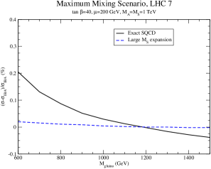
Figure 2: Percentage difference between the Improved Born Approximation and the exact one-loop SQCD calculation of $pp\rightarrow bh$ for maximal mixing in the $b$-squark sector at $\sqrt{s}=7~{}TeV$, $\tan\beta=40$, and $M_{A}=1~{}TeV$.

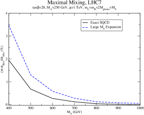
Figure 3: Percentage difference between the Improved Born Approximation and the exact one-loop SQCD calculation of $pp\rightarrow bh$ for maximal mixing in the $b$-squark sector at $\sqrt{s}=7~{}TeV$, $\tan\beta=20$, and $M_{A}=250~{}GeV$.

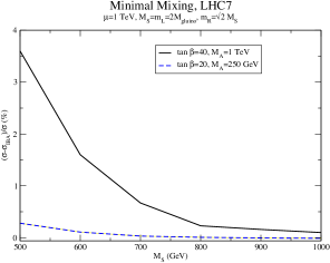
Figure 4: Percentage difference between the Improved Born Approximation and the exact one-loop SQCD calculation for $pp\rightarrow bh$ for minimal mixing in the $b$ squark sector at $\sqrt{s}=7~{}TeV$.

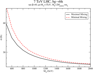
Figure 5: Comparison between the exact one-loop SQCD calculation for $pp\rightarrow bh$ for minimal and maximal mixing in the $b$ squark sector at $\sqrt{s}=7~{}TeV$ and $\tan\beta=40$. The minimal mixing curve has $m_{R}=\sqrt{2}M_{S}$ and ${\tilde{\theta}}_{b}\sim 0$, while the maximal mixing curve has $m_{R}=M_{S}$ and ${\tilde{\theta}}_{b}\sim{\pi\over 4}$.

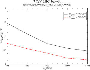
Figure 6: Percentage difference between the Improved Born Approximation and the exact one-loop SQCD calculation for $pp\rightarrow bh$ as a function of $m_{R}$ at $\sqrt{s}=7~{}TeV$ and $\tan\beta=40$.

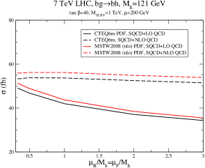
Figure 7: Total cross section for $pp\rightarrow b(\overline{b})h$ production including NLO QCD and SQCD corrections (dotted lines) as a function of renormalization/factorization scale using CTEQ6m (black) and MSTW2008 NLO (red) PDFs. We take $M_{\tilde{g}}=1~{}TeV$ and the remaining MSSM parameters as in Fig. 2.

In Fig. 7, we show the scale dependence for the total rate, including NLO QCD and SQCD corrections (dotted lines) for a representative set of MSSM parameters at $\sqrt{s}=7~{}TeV$. The NLO scale dependence is quite small when $\mu_{R}=\mu_{F}\sim M_{h}$. However, there is a roughly $\sim 5\%$ difference between the predictions found using the CTEQ6m PDFs and the MSTW2008 NLO PDFsMartin et al. (2009). In Fig. 8, we show the scale dependence for small $\mu_{F}$ (as preferred by Maltoni et al. (2005)), and see that it is significantly larger than in Fig. 7. This is consistent with the results of Harlander and Kilgore (2003); Dittmaier et al. (2011).

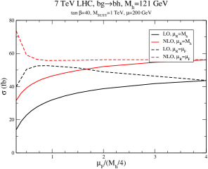
Figure 8: Total cross section for $pp\rightarrow b(\overline{b})h$ production including NLO QCD and SQCD corrections as a function of the factorization scale using MSTW2008 NLO PDFs. We take $M_{\tilde{g}}=1~{}TeV$ and the remaining MSSM parameters as in Fig. 2.

V Conclusion

The analytical and numerical results presented in the previous sections clearly demonstrate that deviations from the $\Delta_{b}$ approximation are suppressed by powers of $(M_{EW}/M_{S})$ in the large $\tan\beta$ region. The $\Delta_{b}$ approximation hence yields an accurate prediction in the $5$ flavor number scheme for the cross section for squark and gluino masses at the TeV scale.

References

- Dittmaier et al. (2011) S. Dittmaier et al. (LHC Higgs Cross Section Working Group) (2011), eprint 1101.0593.
- Benjamin et al. (2010) D. Benjamin et al. (Tevatron New Phenomena and Higgs Working Group) (2010), eprint 1003.3363.
- Chatrchyan et al. (2011) S. Chatrchyan et al. (CMS) (2011), eprint 1104.1619.
- Dawson et al. (2006) S. Dawson, C. B. Jackson, L. Reina, and D. Wackeroth, Mod. Phys. Lett. A21, 89 (2006), eprint hep-ph/0508293.
- Campbell et al. (2004) J. Campbell et al. (2004), eprint hep-ph/0405302.
- Maltoni et al. (2003) F. Maltoni, Z. Sullivan, and S. Willenbrock, Phys. Rev. D67, 093005 (2003), eprint hep-ph/0301033.
- Dawson et al. (2005) S. Dawson, C. B. Jackson, L. Reina, and D. Wackeroth, Phys. Rev. Lett. 94, 031802 (2005), eprint hep-ph/0408077.
- Dittmaier et al. (2004) S. Dittmaier, M. Kramer, and M. Spira, Phys. Rev. D70, 074010 (2004), eprint hep-ph/0309204.
- Dicus et al. (1999) D. Dicus, T. Stelzer, Z. Sullivan, and S. Willenbrock, Phys. Rev. D59, 094016 (1999), eprint hep-ph/9811492.
- Dawson et al. (2004) S. Dawson, C. B. Jackson, L. Reina, and D. Wackeroth, Phys. Rev. D69, 074027 (2004), eprint hep-ph/0311067.
- Maltoni et al. (2005) F. Maltoni, T. McElmurry, and S. Willenbrock, Phys. Rev. D72, 074024 (2005), eprint hep-ph/0505014.
- Campbell et al. (2003) J. Campbell, R. K. Ellis, F. Maltoni, and S. Willenbrock, Phys. Rev. D67, 095002 (2003), eprint hep-ph/0204093.
- Carena et al. (2007) M. S. Carena, A. Menon, and C. E. M. Wagner, Phys. Rev. D76, 035004 (2007), eprint arXiv:0704.1143 [hep-ph].
- Carena et al. (1999) M. S. Carena, S. Mrenna, and C. E. M. Wagner, Phys. Rev. D60, 075010 (1999), eprint hep-ph/9808312.
- Field et al. (2007) B. Field, L. Reina, and C. B. Jackson, Phys. Rev. D76, 074008 (2007), eprint 0705.0035.
- Dawson and Jaiswal (2010) S. Dawson and P. Jaiswal, Phys. Rev. D81, 073008 (2010), eprint 1002.2672.
- Beccaria et al. (2010) M. Beccaria et al., Phys. Rev. D82, 093018 (2010), eprint 1005.0759.
- Dawson and Jackson (2008) S. Dawson and C. B. Jackson, Phys. Rev. D77, 015019 (2008), eprint 0709.4519.
- Dabelstein (1995) A. Dabelstein, Nucl. Phys. B456, 25 (1995), eprint hep-ph/9503443.
- Hall et al. (1994) L. J. Hall, R. Rattazzi, and U. Sarid, Phys. Rev. D50, 7048 (1994), eprint hep-ph/9306309.
- Carena et al. (2000) M. S. Carena, D. Garcia, U. Nierste, and C. E. M. Wagner, Nucl. Phys. B577, 88 (2000), eprint hep-ph/9912516.
- Guasch et al. (2003) J. Guasch, P. Hafliger, and M. Spira, Phys. Rev. D68, 115001 (2003), eprint hep-ph/0305101.
- Haber et al. (2001) H. E. Haber et al., Phys. Rev. D63, 055004 (2001), eprint hep-ph/0007006.
- Harlander and Kilgore (2003) R. V. Harlander and W. B. Kilgore, Phys. Rev. D68, 013001 (2003), eprint hep-ph/0304035.
- Heinemeyer et al. (2005) S. Heinemeyer, W. Hollik, H. Rzehak, and G. Weiglein, Eur. Phys. J. C39, 465 (2005), eprint hep-ph/0411114.
- Brignole et al. (2002) A. Brignole, G. Degrassi, P. Slavich, and F. Zwirner, Nucl. Phys. B643, 79 (2002), eprint hep-ph/0206101.
- Noth and Spira (2010) D. Noth and M. Spira (2010), eprint 1001.1935.
- Noth and Spira (2008) D. Noth and M. Spira, Phys. Rev. Lett. 101, 181801 (2008), eprint 0808.0087.
- Dittmaier et al. (2007) S. Dittmaier, M. Kramer, A. Muck, and T. Schluter, JHEP 03, 114 (2007), eprint hep-ph/0611353.
- Dawson et al. (2011) S. Dawson, C. Jackson, and P. Jaiswal, Phys.Rev. D83, 115007 (2011), eprint 1104.1631.
- Carena et al. (1994) M. S. Carena, M. Olechowski, S. Pokorski, and C. E. M. Wagner, Nucl. Phys. B426, 269 (1994), eprint hep-ph/9402253.
- Berger et al. (2005) E. L. Berger, T. Han, J. Jiang, and T. Plehn, Phys. Rev. D71, 115012 (2005), eprint hep-ph/0312286.
- Dittmaier et al. (2009) S. Dittmaier, M. Kramer, M. Spira, and M. Walser (2009), eprint 0906.2648.
- Nadolsky et al. (2008) P. M. Nadolsky et al., Phys. Rev. D78, 013004 (2008), eprint 0802.0007.
- Martin et al. (2009) A. D. Martin, W. J. Stirling, R. S. Thorne, and G. Watt, Eur. Phys. J. C63, 189 (2009), eprint 0901.0002.