Corner free energies and boundary effects for Ising, Potts and fully-packed loop models on the square and triangular lattices

Abstract

We obtain long series expansions for the bulk, surface and corner free energies for several two-dimensional statistical models, by combining Enting’s finite lattice method (FLM) with exact transfer matrix enumerations. The models encompass all integrable curves of the $Q$-state Potts model on the square and triangular lattices, including the antiferromagnetic transition curves and the Ising model ($Q=2$) at temperature $T$, as well as a fully-packed O($n$) type loop model on the square lattice. The expansions are around the trivial fixed points at infinite $Q$, $n$ or $1/T$.

By using a carefully chosen expansion parameter, $q\ll 1$, all expansions turn out to be of the form $\prod_{k=1}^{\infty}(1-q^{k})^{\alpha_{k}+k\beta_{k}}$, where the coefficients $\alpha_{k}$ and $\beta_{k}$ are periodic functions of $k$. Thanks to this periodicity property we can conjecture the form of the expansions to all orders (except in a few cases where the periodicity is too large). These expressions are then valid for all $0\leq q<1$.

We analyse in detail the $q\to 1^{-}$ limit in which the models become critical. In this limit the divergence of the corner free energy defines a universal term which can be compared with the conformal field theory (CFT) predictions of Cardy and Peschel. This allows us to deduce the asymptotic expressions for the correlation length in several cases.

Finally we work out the FLM formulae for the case where some of the system’s boundaries are endowed with particular (non-free) boundary conditions. We apply this in particular to the square-lattice Potts model with Jacobsen-Saleur boundary conditions, conjecturing the expansions of the surface and corner free energies to arbitrary order for any integer value of the boundary interaction parameter $r$. These results are in turn compared with CFT predictions.

,

1 Introduction

Over the years much effort has been devoted to the study of boundary effects in statistical models. In the particular case of critical two-dimensional systems a huge amount of knowledge has been obtained by the application of the powerful techniques of integrability and conformal field theory (CFT) [1, 2]. The critical fluctuations near a boundary have been shown to define various boundary critical exponents, many of which can be computed exactly.

Once a model has been shown to be exactly solvable (integrable), it is usually rather simple to obtain the dominant asymptotics for the partition function, i.e., the bulk free energy $f_{\rm b}$. The usual route is to diagonalise the transfer matrix in a cylinder geometry, using the Bethe Ansatz, and to extract its dominant eigenvalue in the thermodynamic limit. Similarly, if the boundary conditions are compatible with integrability (in the sense of Sklyanin’s reflection equation [3]) one can diagonalise the transfer matrix in a strip geometry and retrieve the surface free energy $f_{\rm s}$. Obviously $f_{\rm b}$ and $f_{\rm s}$ give important information about the particular lattice model being studied. However, both quantities are non-universal and as such teach us nothing about the critical system that emerges in the continuum limit.

If the lattice model under study is defined on a large rectangle, the next subdominant contribution to the free energy comes from the corners. Cardy and Peschel [4] have shown that this corner free energy $f_{\rm c}$ is of universal nature. Indeed it contains information about the central charge $c$ of the field theory that governs the continuum limit.

Unfortunately only very little is known about $f_{\rm c}$ from the point of view of exactly solvable models. To compute it from the Bethe Ansatz would require knowledge about how to implement a given boundary condition in terms of Bethe states. Typically this would call for information about all the eigenstates, not just the one defining the leading eigenvalue. This obviously defines a very hard problem which, as far as we know, has not yet been addressed.

One of the authors has recently conjectured exact product formulae for ${\rm e}^{f_{\rm b}}$, ${\rm e}^{f_{\rm s}}$ and ${\rm e}^{f_{\rm c}}$ in a particular two-dimensional model, viz. the zero-temperature antiferromagnetic $Q$-state Potts model on the triangular lattice [5]. To obtain these expressions, the first step was to compute the first 40 terms of their large-$Q$ expansion, by combining Enting’s finite lattice method (FLM) [6] with exact transfer matrix enumerations. The next step was to notice that when reexpressed in terms of the variable $x\ll 1$ defined by $Q=2-x-x^{-1}$ these series could be rewritten as product formulae of the type

$$\prod_{k=1}^{\infty}(1-x^{k})^{\alpha_{k}}\,,$$ (1)

where crucially the exponents $\alpha_{k}$ turned out to be periodic functions of $k$. Since the observed periods (6 for $f_{\rm b}$, and 12 for $f_{\rm s}$ and $f_{\rm c}$) were much shorter than the number of available terms, it then became feasible to conjecture the exact product formulae, valid for any $x$ in the range $0\leq x<1$. The model is non-critical in that range, but goes to a critical theory when $x\to 1^{-}$ (i.e., $Q\to 4^{+}$).

The purpose of this paper is to extend this type of results to a whole range of two-dimensional lattice models. We recall the definitions of the models to be studied in section 2 below. They encompass all integrable curves of the $Q$-state Potts model on the square and triangular lattices, including the antiferromagnetic transition curves and the Ising model ($Q=2$) at temperature $T$, as well as a fully-packed O($n$) type loop model on the square lattice. The expansions are around the trivial fixed points at infinite $Q$, $n$ or $1/T$.

A crucial ingredient in carrying out this programme is obviously to identify the correct expansion variable $x$ (that we shall call $q$ in the general case). We wish $q$ to have the property that the model is trivial for $q=0$, non-critical for $0\leq q<1$, and critical in the limit $q\to 1^{-}$. Below we shall focus only on models which are known to be integrable (at least in the bulk), and we can therefore take inspiration for the choice of $q$ from the exact solution (for the bulk properties). Incidentally, we have no reason to believe that nice product formulae hold for models that are not integrable.

In all cases that we have investigated, it appears that ${\rm e}^{f_{\rm b}}$, ${\rm e}^{f_{\rm s}}$ and ${\rm e}^{f_{\rm c}}$ can be cast as exact product formulae of the more general form

$$\prod_{k=1}^{\infty}(1-q^{k})^{\alpha_{k}}\,,\qquad\mbox{with }\alpha_{k}=\beta_{k}k+\gamma_{k}\,,$$ (2)

where both sets of coefficients $\beta_{k}$ and $\gamma_{k}$ are periodic functions of $k$ with the same period. We find for all Potts and fully-packed loop models included in this study that the period associated with ${\rm e}^{f_{\rm s}}$ and ${\rm e}^{f_{\rm c}}$ is precisely twice the period associated with ${\rm e}^{f_{\rm b}}$. For Ising models we find on the contrary that all three quantities have the same period. At present we have no satisfactory explanation for this observation of period doubling for the boundary related properties.

Just like in [5] we can then conjecture the exact product formula, provided that the series obtained from the FLM has sufficiently many terms to cover at least one period (plus a few extra terms to verify the assumption of periodicity, and to account for some simple extra factors in front of the product which are sometimes present). Only in a few exceptional cases do the series turn out to be too short, but we can then at least state how many further terms would be needed in order to establish the product form.

The organisation of the paper is as follows. In section 2 we precisely define the models to be studied in this paper. In section 3 we first review the FLM for models with free boundary conditions. Then we present our main results in the form of product formulae for the bulk, surface and corner free energies of the various models. We give details about the period doubling phenomenon for the boundary related properties. When studying the critical limit $q\to 1^{-}$ we pay special attention to the divergence of the corner free energy, since this can be compared with CFT results [4]. As a by-product we obtain results about the asymptotic behaviour of the correlation length.

In section 4 we study the effect of imposing particular (non-free) boundary conditions on some of the system’s boundaries. We adapt the FLM formalism to this case and separate the contributions from corners of different types, i.e., where two free (resp. two particular, resp. one free and one particular) boundary conditions meet. It is shown analytically that the contributions to the free energy from corners of different types simply add up, as expected for an inherently non-critical system. We apply this formalism to a family of Potts-model boundary conditions recently introduced by Jacobsen and Saleur (JS) [7] in which a parameter $r$ controls the weight of Fortuin-Kasteleyn clusters that touch the particularised boundaries. Explicit results are obtained for any integer value of $r$. To finish, we comment on the relation with CFT results for such boundary conditions.

2 Models

In this section we define the models to be studied in this paper and briefly review their most relevant properties. These models constitute all integrable cases of the Potts model on the square and triangular lattices. We also study a model of two mutually excluding sets of fully-packed loops, known as the ${\rm FPL}^{2}$ model [8].

In the entire paper we will define the (dimensionless) free energy as the logarithm of the partition function, $f\equiv\ln Z$, i.e., without the conventional minus sign.

2.1 Potts model: generalities

Let us recall that the $Q$-state Potts model is a model of interacting spins on a lattice, allowing each spin to be in one among $Q$ different states, and such that the interaction between neighbouring spins depends only on whether they are in the same or different states. The underlying lattice, or graph, is denoted as $G=(V,E)$, where $V$ (resp. $E$) is the set of vertices (resp. edges). The associated (dimensionless) hamiltonian thus reads

$$\beta H=-K\sum_{(i,j)\in E}\delta_{\sigma_{i},\sigma_{j}}\,,\qquad\sigma_{i}=1,\ldots,Q\,,$$ (3)

where $K=J/k_{B}T$ is the (dimensionless) coupling constant.

It is well-known that the partition function can be rewritten as [9]

$$Z=\sum_{A\subseteq E}Q^{k(A)}v^{|A|}\,,$$ (4)

where the sum runs over subsets $A$ (of cardinality $|A|$) of the lattice edges $E$. Each connected component in $A$ is known as a Fortuin-Kasteleyn (FK) cluster, and $k(A)$ denotes the number of connected components. The temperature parameter $v$ is defined as $v={\rm e}^{K}-1$.

Obviously, the FK formulation makes sense also when $Q$ is an arbitrary real number. Suppose now that the Potts model is defined on an infinite regular lattice ($|V|,|E|\to\infty$) with coordination number $z=2|E|/|V|$. If we study the model on some curve in the $(Q,v)$ plane with asymptotics

$$v\sim Q^{2/z}\qquad\mbox{for }|Q|\gg 1\,,$$ (5)

then there will be precisely two dominant contributions to $Z$: $A=E$ (with $k(A)=1$) and $A=\emptyset$ (with $k(A)=|V|$). In other words, there is phase coexistence between the low-temperature and high-temperature phases. All subdominant contributions can be written perturbatively as powers of the small parameter $1/Q$. This perturbative picture is the starting point for making series expansions of the free energy.

2.2 Lattices and their orientation

In a detailed study of boundary effects it is important to specify not only on which regular lattice the model is defined, but also how the boundaries are oriented with respect to the lattice’s symmetry axes.

Moreover, we do not expect that the free energy series can be written as nice product formulae of the type (2) for an arbitrary lattice model of interest. The model will in general have to be integrable to yield nice expressions. We recall that a model remains integrable in the presence of boundaries, only if the boundary conditions satisfy the reflection equation [3]. This places strong constraints on how the boundaries can be oriented.

Figure 1: Different types of lattices to be used throughout this work. From left to right: a) square lattice in a rectangle of size $M\times N$, b) triangular lattice in a (deformed) rectangle of size $M\times N$, and c) triangular lattice in an equilateral triangle of size $M$.

The Potts model on the square and triangular lattices is integrable for certain curves in the $(Q,v)$ plane, which we briefly review below. Boundary integrability turns out to hold as well, provided that the boundaries are oriented parallel to the principal axes of the lattice. In particular, an $M\times N$ rectangular piece of the square lattice will be oriented as shown in Fig. 1a.

When dealing with a triangular lattice, we can again take an $M\times N$ (deformed) rectangular piece, as shown in Fig. 1b. This lattice can be considered simply as a square lattice with added diagonals. This point of view is often convenient, since then the FLM formulae can be taken over from the square-lattice case, and the transfer matrix algorithms need only very minor modifications.

There is however one disadvantage: since the four corners are not equivalent, the corner free energy will be a mixture of two contributions from corners sustaining an angle $\pi/3$ and two contributions from $2\pi/3$ corners. To separate these contributions we shall find it advantageous to consider as well the triangular lattice inscribed in an equilateral triangle of side length $M$, as shown in Fig. 1c. This involves three $\pi/3$ corners, but makes both the FLM formulae and the transfer matrix algorithms slightly less performing.

2.3 Square-lattice Potts model

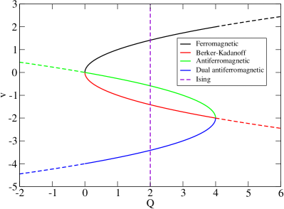
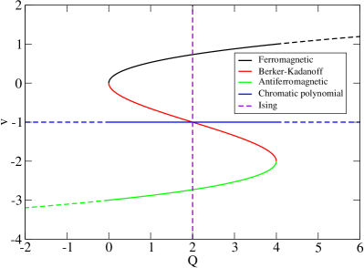
Figure 2: Phase diagrams in the $(Q,v)$ plane of the Potts model on a) the square lattice, and b) the triangular lattice. The models are integrable along the curves shown. Critical (resp. non-critical) behaviour is signalled by solid (resp. dashed) line style. For further details on these curves, their properties and nomenclature, and the renormalisation group flows, the reader can consult [10, 11] and references therein.

The phase diagram of the square-lattice Potts model is shown in Fig. 2a. The model is integrable [12] along the selfdual curves

$$v=\pm\sqrt{Q}\,,$$ (6)

corresponding to a critical (resp. non-critical) theory for $0\leq Q\leq 4$ (resp. $Q>4$). The conformal properties in the critical regime are known [13]. The only simple property that we need here is that the point $(Q,v)=(4,2)$ is critical with central charge $c=1$.

Note that (6) satisfies the criterion (5), thus making possible a perturbative expansion for $Q\gg 1$. We shall see below that this expansion enables us to attain the point $(Q,v)=(4,2)$ as an appropriate limit.

The square-lattice Potts model is also integrable [14] along the mutually dual antiferromagnetic curves

$$v=-2\pm\sqrt{4-Q}\,,$$ (7)

corresponding to a critical (resp. non-critical) theory for $0\leq Q\leq 4$ (resp. $Q<0$).

The conformal properties along (7) are quite intricate, but much is known [10, 11, 15, 16]. In particular one has $c=-1$ in the limit $(Q,v)\to(0,0)$. Since (7) again satisfies (5) the perturbative expansion enables us to attain this point as an appropriate limit.

Note finally that the $Q$-state Potts model is equivalent to a problem of self-avoiding loops [17]. The loops are defined on the medial lattice and each one carries a weight $n=\sqrt{Q}$. The loop formulation can further be brought in equivalence with the six-vertex model [17]. The six-vertex model is homogeneous on the curve (6) and staggered on (7) [18].

2.4 Triangular-lattice Potts model

The phase diagram of the triangular-lattice Potts model is shown in Fig. 2b. The model is integrable along the cubic curve [19]

$$v^{3}+3v^{2}=Q\,.$$ (8)

Once again (5) is satisfied.

For $0\leq Q\leq 4$ the critical behaviour for $v\geq 0$ (i.e., along the upper branch of (8)) coincides with that of the square lattice. Along the lower branch of (8) one finds [11] the same critical behaviour as on the antiferromagnetic curve (7) on the square lattice.

The two critical points that can be accessed perturbatively are $(Q,v)=(4,1)$ with $c=1$, and $(Q,v)\to(0,-2)$ with $c=-1$ [11].

We shall sometimes refer to (8) as the selfdual curve. Indeed, if one combines a duality transformation of the triangular-lattice Potts model with a partial summation (decimation) over one half of the spins in the dual model on the hexagonal lattice, the result is a non-trivial transformation whose fixed points are exactly (8). In this sense the nomenclature “selfdual” is justified when speaking about the curve (8).

In the special case $v=-1$ and any real $Q$, the Potts partition function $Z$ (4) reduces to the so-called chromatic polynomial. For integer $Q$ this can be interpreted as a colouring problem. To be precise, $Z$ equals the number of proper vertex colourings of the lattice, i.e., assignations to each of the vertices in $G$ of one among the $Q$ different colours, in such a way that adjacent vertices carry different colours.

The chromatic polynomial is integrable [20, 21] for any real $Q$. It corresponds to a critical theory if and only if $0\leq Q\leq 4$. Its phase diagram within the critical phase is complicated [21] and has been reviewed in [22]. The only properties that we shall need here are that the point $(Q,v)=(4,-1)$ has $c=2$, while the limit $(Q,v)\to(0,-1)$ corresponds to $c=-1$.

The bulk, surface and corner free energies for the chromatic polynomial on the triangular lattice have already been discussed in [5]. In section 3.2.4 we shall however be able to go beyond these results and separate the contributions to the corner free energy for two different types of corners (of angles $\frac{2\pi}{3}$ and $\frac{\pi}{3}$).

2.5 Ising model

For $Q=2$ the Potts model reduces to the Ising model with (dimensionless) hamiltonian

$$\beta H=-K_{\rm Ising}\sum_{(i,j)\in E}S_{i}S_{j}\,,\qquad S_{i}=\pm 1\,.$$ (9)

The coupling constants in (3) and (9) are obviously related by $K_{\rm Ising}=\frac{1}{2}K$.

The Ising model is integrable at any temperature on both the square and the triangular lattices [18]. We shall only be interested in the cases $K_{\rm Ising}>0$. The critical point on the ferromagnetic critical curves is situated at $K_{\rm Ising}=\frac{1}{2}\log(1+\sqrt{2})$ on the square lattice (see Fig. 2a) and at $K_{\rm Ising}=\frac{1}{4}\log 3$ on the triangular lattice (see Fig. 2b). The low-temperature perturbative expansion gives access to the critical point in an appropriate limit.

When studying the Ising model, we will always treat it as a Potts model and rewrite $K_{\rm Ising}$ in terms of $K$.

2.6 ${\rm FPL}^{2}$ model

Apart from the special cases of Potts models described above, we also consider a model of two mutually excluding sets of fully-packed loops on the square lattice, known as the ${\rm FPL}^{2}$ model [8]. The allowed configurations are such that each vertex is in one of the six states shown in Fig. 3. A weight $n_{1}$ (resp. $n_{2}$) is associated with each black (resp. red) loop.

Figure 3: Allowed vertex states in the FPL² model.

The ${\rm FPL}^{2}$ model is integrable when the two weights are equal, $n_{1}=n_{2}\equiv n$ [23, 24, 25]. We study henceforth only this integrable case. It gives rise to a critical (resp. non-critical) model when $-2\leq n\leq 2$ (resp. $|n|>2$).

When the FPL² model is defined on a bipartite 4-regular lattice, its configurations are in bijection with those of a 3-dimensional interface model on the dual lattice [8]. This allows for the redistribution of the loop weights $n_{1}$ and $n_{2}$ as local complex vertex weights. In the critical regime the resulting local formulation is the key to the exact derivation of the critical exponents by the Coulomb gas method [26, 27].

Figure 4: A finite bipartite 4-regular lattice of width $M=3$ and height $N=2$.

To investigate the surface properties of the FPL² model without breaking any symmetries (which might lead to a change of universality class) one therefore needs to define it on a finite lattice which is bipartite and 4-regular [28]. An appropriate choice of lattice is shown in Fig. 4.

3 Bulk, surface and corner free energies with free boundary conditions

In this section, we compute the bulk, surface and corner free energies of each of the considered models in the case of lattices with free boundary conditions. Achieving the goals described in the Introduction relies in all cases on writing these free energies as power series in terms of some good perturbative parameter. Long series are then generated by combining transfer matrix techniques with the use of Enting’s finite lattice method [6], which we first review below.

For each model being considered, the first term of the series expansion is some unique (or sometimes twofold degenerate) ground state. As mentioned at the end of section 2.3 we shall treat the Potts models (4) in terms of the equivalent loop models on the medial lattice. The ground state is then chosen as the unique state in which one loop surrounds each vertex in the original lattice $G$; see Fig. 5. Equivalently, the edge subset $A\subseteq E$ appearing in (4) is empty, $A=\emptyset$.

Similarly, for the Ising model the ground state is chosen as one of the two equivalent ferromagnetic states with all spins pointing in the same direction.

Figure 5: Representation of the ground state used as a basis for the finite lattice method (left), and of one of the first excitations to be taken into account in the series expansion (right), in the case of the square-lattice Potts model. The black edges on the right correspond to the subset $A\subseteq E$ appearing in (4). The blue box surrounding $A$ corresponds to the smallest finite sublattice $[i,j]$ in which this excitation appears.

For the ferromagnetic Potts model (both on the square and triangular lattices), the chromatic polynomial on the triangular lattice, or for the ${\rm FPL}^{2}$ model, a good expansion parameter will turn out to be, rather than the inverse $n^{-1}$ of the loop fugacity ($n\equiv\sqrt{Q}$), the parameter $q$ defined by

$$\sqrt{Q}=q+\frac{1}{q}\,.$$ (10)

Actually, for these models $q$ is nothing but the quantum group deformation parameter. Indeed, all these Potts models present a quantum group symmetry $U_{q}(sl_{2})$. The ${\rm FPL}^{2}$ model is endowed with the larger symmetry $U_{q}(sl_{4})$.

For the critical antiferromagnetic Potts model on the square lattice the suitable parameter $q$ is defined by

$$Q=-\left(q-\frac{1}{q}\right)^{2}\,.$$ (11)

Finally, for the Ising model the choice of the expansion parameter $q$ is far less obvious. Indeed, the approach outlined in the Introduction makes it necessary that the critical point correspond to the limit $q\to 1^{-}$. The correct choice of $q$ then involves parameterising the coupling constant in terms of suitable elliptic functions, as in Baxter’s analytical results [29, 18]. We defer further details to the corresponding sections below.

3.1 FLM for lattices with free boundary conditions

We now outline the principles of the FLM for lattices with free boundary conditions. The formalism depends on the choice of regular polygons in which the excitations over the ground state are inscribed. The most common and well-known choice is rectangles, as illustrated by the blue box in Fig. 5. We review this first (in section 3.1.1) for convenience, and in order to fix the notation. Then, in section 3.1.2, we derive the required modifications for the case of triangular lattices with excitations inscribed in equilateral triangles, cf. Fig. 1c.

3.1.1 Lattices inscribed in a rectangle.

We here give a brief review of the earlier work by Enting [6] concerning the basis of the finite lattice method. The FLM allows one to compute the free energies of statistical models defined on an infinite rectangular lattice as a series expansion in terms of finite rectangular graphs. Apart from the square lattice, this method can also be applied to the triangular lattice, which is then considered as a square lattice with added diagonals; see Fig. 1b.

In practice, we will make extensive use of the FLM to approximate the bulk, surface and corner free energies of an infinite $M\times N$ lattice, such as depicted in Fig. 1a–b, from free energies for finite $m\times n$ lattices. The latter are computed by using numerical (but exact) transfer matrix enumerations. The bigger the $m\times n$ lattices whose partition function can be computed numerically, the longer will be the resulting FLM series.

The basic idea underlying the FLM is to write the free energy for the $M\times N$ lattice as a sum over all possible sublattices,

$$f_{M,N}=\sum_{[i,j]\subset[M,N]}{\tilde{f}_{i,j}}=\sum_{i\leq M,j\leq N}{(M-i+1)(N-j+1)\tilde{f}_{i,j}}\,,$$ (12)

where the notation $[i,j]\subset[M,N]$ means that the summation is performed over all sublattices of size $i\times j$ that lie inside the $M\times N$ lattice. The contributions $\tilde{f}_{i,j}$—that must not be confused with the $[i,j]$ lattices’ free energies $f_{i,j}$—are defined self-consistently as functions of the latter by inverting the equation

$$f_{m,n}=\sum_{[i,j]\subset[m,n]}{\tilde{f}_{i,j}}=\sum_{i\leq m,j\leq n}{(m-i+1)(n-j+1)\tilde{f}_{i,j}}\,.$$ (13)

This results in

$$\tilde{f}_{i,j}=\sum_{m\leq i,n\leq j}{f_{m,n}\eta(m,i)\eta(n,js)}\,,$$ (14)

where the functions $\eta$ are defined by Enting [6] as

$$\eta(m,i)=\left\{\begin{array}[]{ll}1&\mbox{ if }m=i\mbox{ or }m+2=i\mbox{ and }i>2\,,\\ 2&\mbox{ if }m+1=i\mbox{ and }i>1\,,\\ 0&\mbox{ otherwise.}\end{array}\right.$$ (15)

For an infinite $M\times N$ lattice, the sum (12) is restricted to a certain range of finite $m\times n$ sublattices by imposing some cutoff set. In the course of this paper, and as prescribed in [6], this cutoff set is chosen to be

$$B(k)=\left\{[m,n]\,,m+n=k\right\}\,.$$ (16)

Hence, (12) formally reads

$$f_{M,N}\approx\sum_{[i,j]\leq B(k)}{(M-i+1)(N-j+1)\tilde{f}_{i,j}}\,,$$ (17)

which is generally shown to give an approximation of $f_{M,N}$ up to an order increasing with $k$ in terms of some good perturbative parameter, as discussed above and detailed in the following sections.

The free energy (17) can be written as the sum of a bulk contribution $MNf_{\rm b}$, a surface contribution $(M+N)f_{\rm s}$, and a corner contribution $f_{\rm c}$, that is

$$f_{M,N}=MNf_{\rm b}+(M+N)f_{\rm s}+f_{\rm c}$$ (18)

These three contributions can be computed separately. The final form of the FLM expansions with cutoff $B(k)$ come out as [6]

$$f_{\rm b} = \sum_{[m,n]\leq B(k)}f_{m,n}\big{(}\delta_{m,k-n}-3\delta_{m,k-n-1}+3\delta_{m,k-n-2}-\delta_{m,k-n-3}\big{)}\,,$$

$$f_{\rm s} = \sum_{[m,n]\leq B(k)}f_{m,n}\big{(}(1-m)\delta_{m,k-n}+(3m-1)\delta_{m,k-n-1}\,,$$ (19)

$$\qquad-(3m+1)\delta_{m,k-n-2}+(m+1)\delta_{m,k-n-3}\big{)}$$

$$f_{\rm c} = \sum_{[m,n]\leq B(k)}f_{m,n}\big{(}(m-1)(n-1)\delta_{m,k-n}+(1+m+n-3mn)\delta_{m,k-n-1}$$

$$\qquad+(3mn+m+n-1)\delta_{m,k-n-2}-(m+1)(n+1)\delta_{m,k-n-3}\big{)}\,,$$

where all the $f_{m,n}$ with $m$ or $n$ non-positive are zero by convention. Compared to Enting’s formulae, the expression for $f_{\rm s}$ has been simplified under the assumption that the $f_{m,n}$ are symmetric in $m$ and $n$, which will always be the case in this paper.

3.1.2 Triangular lattices in triangles.

For the sake of studying models defined on the triangular lattice, it is sometimes useful to work with only one type of corners. One then seeks the free energy $f_{M}$ of the model defined on a large equilateral triangle of side $M$, as shown in Fig. 1c. We have derived the corresponding FLM formulae, going through the same steps as above.

The starting point is now

$$f_{M}\approx\sum_{i\leq k}{\frac{(M-i+1)(M-i+1)}{2}\tilde{f}_{i}}\,,$$ (20)

where the self-consistency condition

$$f_{m}=\sum_{i\leq m}{\frac{(m-i+1)(m-i+1)}{2}\tilde{f}_{i}}$$ (21)

yields

$$\tilde{f}_{i}=\sum_{m\leq i}f_{m}(\delta_{m,i}-3\delta_{m,i-1}+3\delta_{m,i-2}-\delta_{m,i-3})\,.$$ (22)

Finally, the free energy is written as

$$f_{M}=\frac{M(M+1)}{2}f_{\rm b}+Mf_{\rm s}+f_{\rm c}\,,$$ (23)

where the different contributions are given by

$$f_{\rm b} = \sum_{m\leq k}f_{m}\big{(}\delta_{m,k}-2\delta_{m,k-1}+\delta_{m,k-2}\big{)}\,,$$

$$f_{\rm s} = \sum_{m\leq k}f_{m}\big{(}(1-m)\delta_{m,k}+(2m+1)\delta_{m,k-1}-(m+2)\delta_{m,k-2}\big{)}\,,$$ (24)

$$f_{\rm c} = \frac{1}{2}\sum_{m\leq k}f_{m}\big{(}(m^{2}-3m+2)\delta_{m,k}+2(1-m^{2})\delta_{m,k-1}$$

$$\qquad+(m^{2}+3m+2)\delta_{m,k-2}\big{)}\,.$$

3.2 Results

3.2.1 Selfdual Potts model on the square lattice.

On its selfdual curve, the square-lattice Potts model is equivalent to a loop model, where each loop carries a statistical weight $n=\sqrt{Q}$. The partition functions of finite lattices of size $M\times N$ reads

$$Z_{M,N}=n^{MN}P_{d}(n^{-1})\,,$$ (25)

where $P_{d}(x)$ is a polynomial of degree $d=MN-1$. The constant coefficient $P_{d}(0)=1$ corresponds to the ground state shown in Fig. 5a.

The FLM formulae thus reduce to an expansion in powers of $1/n$, which is correct up to an order determined by the size of the graph with highest weight that cannot fit into the cutoff set $B(k)$. Compared to the ground state configuration, this property is satisfied by the graphs in which the edge subset $A\subset E$ of (4) forms one straight or L-shaped figure of total length $k+1$, which contribute to the order $n^{-k}$. We thus expect the FLM formulae (19) with a cutoff $B(k)$ to give an approximation of the $M\times N$ free energy that is correct up to order $n^{-k}$.

Using a transfer matrix algorithm, we have computed the polynomials $P_{d}(x)$ for all finite lattices within the cutoff set $B(31)$, allowing correct results up to order $n^{-31}$.

Using instead of $1/n$ the small parameter $q$ defined by

$$n=q+\frac{1}{q}$$ (26)

the exponentiated free energies $\rme^{f_{\rm b}}$, $\rme^{f_{\rm s}}$ and $\rme^{f_{\rm c}}$ finally turn out to have up to this order the following nice expressions

$$\rme^{f_{\rm b}} = \frac{q^{2}+1}{q^{2}(q-1)^{2}}\prod_{k=1}^{\infty}{\left(\frac{1-q^{4k-1}}{1-q^{4k+1}}\right)^{4}}\,,$$

$$\rme^{f_{\rm s}} = (1-q)\prod_{k=1}^{\infty}{\left(\frac{1-q^{8k-1}}{1-q^{8k-5}}\right)^{2}}\,,$$ (27)

$$\rme^{f_{\rm c}} = \prod_{k=1}^{\infty}{\frac{1}{(1-q^{8k-6})(1-q^{8k-4})^{4}(1-q^{8k-2})}}\,.$$

The expression for $\rme^{f_{\rm b}}$ is shown in A to be equivalent to the analytical expression given by Baxter in [18], that is

$$\psi=-\frac{1}{2}\ln Q-2\left[\beta+\sum_{k=1}^{\infty}{\frac{1}{k}\rme^{-k\lambda}\frac{\sinh 2k\beta}{\cosh k\lambda}}\right]\,,$$ (28)

where $\psi\equiv-\lim_{N\to\infty}\frac{1}{N}\ln Z_{N}$ is defined as the dimensionless free energy in the thermodynamic limit (here $Z_{N}$ denotes the partition function of a system with $N$ spins). The correspondence with our notation is

$$\psi = -f_{\rm b}\,,$$

$$Q^{1/2} = 2\cosh\lambda\,,$$

$$\frac{v}{Q^{1/2}} = \frac{\sinh\beta}{\sinh(\beta-\lambda)}\,.$$

The regular form exhibited by the product expression for $\rme^{f_{\rm b}}$—which is proved starting from Baxter’s result (28) in A.1—and its structural similarity with the corresponding conjectured expressions for $\rme^{f_{\rm s}}$ and $\rme^{f_{\rm c}}$ encourages us to assume that the two latter expressions are also valid to all orders. These expressions are, as far as we know, new.

In general we expect $\rme^{f_{\rm b}}$, $\rme^{f_{\rm s}}$ and $\rme^{f_{\rm c}}$ for all the models studied in this paper to have an expression of the form (2), modulo some simple overall factors such as $\frac{q^{2}+1}{q^{2}(q-1)^{2}}$ or $(1-q)$ appearing in (27). Moreover, we expect the coefficients $\beta_{k}$ and $\gamma_{k}$ to be periodic functions of $k$. For instance the results found in (27) correspond to the simplest case of $\beta_{k}=0$; and the periodicities are $4$ for $\rme^{f_{\rm b}}$, and $8$ for $\rme^{f_{\rm s}}$ and $\rme^{f_{\rm c}}$. We shall discuss the issue of periodicity further in section 3.2.8.

The above assumption will be further corroborated by the study of other models in the remainder of the paper.

We remark that a result such as $\rme^{f_{\rm c}}$ in (27) can be said to be established beyond any reasonable doubt, since the coefficients $\gamma_{0},\gamma_{1},\ldots,\gamma_{31}$ determined numerically cover four complete periods. Once the periodicity property is established (or assumed) the determination of the coefficients over a single period (or a little more to be sure) would be sufficient.

One more important feature of the generic form (2) is that it gives a particular meaning to the limit $q\to 1^{-}$, which turns out to be critical for all the considered models. The convergence of products of the type (2) when $q\to 1^{-}$ indeed depends in a non-obvious way on the coefficients $\alpha_{k}$, giving rise to different critical behaviours to be studied in the following.

3.2.2 Antiferromagnetic Potts model on the square lattice.

The antiferromagnetic transition curve [14] for the square-lattice Potts model is given by (7). To resolve the square root we parameterise $Q=-(q^{-1}-q)^{2}$, with $q$ taking real (resp. complex) values in the non-critical (resp. critical) regime. We have then $v=(q^{1/2}-q^{-1/2})^{2}$. This allows us to compute the partition function of finite lattices as polynomials in $q$. More precisely, the partition functions for lattices of size $M\times N$ read

$$Z_{MN}=\frac{q^{M+N-3MN}}{(q^{-1}-q)^{MN}}P_{d}(q)\,,$$ (29)

where $P_{d}(q)$ is a polynomial of degree $d=3MN-M-N$ in $q$ with constant coefficient $P_{d}(0)=1$. To obtain $P_{d}$, FLM calculations are applied in exactly the same way as for the selfdual curve. The numerical calculations are now done up to order $q^{22}$, i.e., using the finite partition functions with the cutoff set $B(23)$. This gives for the bulk, surface and corner and free energies:

$$\rme^{f_{\rm b}} = -\frac{(1-q)^{2}(1-q^{2})}{q^{2}}\prod_{k=1}^{\infty}{\left(\frac{1-q^{8k-2}}{1-q^{8k-6}}\right)^{2}}\,,$$

$$\rme^{f_{\rm s}} = \frac{1}{(1-q)}\prod_{k=1}^{\infty}{\frac{(1-q^{16k-14})(1-q^{16k-2})}{(1-q^{16k-10})(1-q^{16k-6})}}\prod_{k=1}^{\infty}{\left(\frac{1-q^{8k-3}}{1-q^{8k+1}}\right)^{2}}\,,$$ (30)

$$\rme^{f_{\rm c}} = \prod_{k=1}^{\infty}\frac{(1-q^{4k-2})(1-q^{8k-4})^{3}}{(1-q^{16k-8})^{4}}\,.$$

The presence of an overall minus sign in ${\rm e}^{f_{\rm b}}$ stems from the fact that $Q<0$, and should not be taken into account as for the critical properties of the model when $Q\to 0$. The expression found for $\rme^{f_{\rm b}}$ is shown in A.2 to be equivalent to an expression given by Baxter in section 12.5 of [14], up to an analytic continuation. More precisely, using the same notations as for the self-dual case, the free energy $\psi$ is given for $Q\geq 4$ by (28), where this time $\beta$ has to be replaced by a parameter $u$ defined by

$${\rm e}^{K}=\frac{\sinh(\lambda+u)}{\sinh(\lambda-u)}\,,\qquad 0\leq\Im u<\pi\,,$$ (31)

the expression being valid under the condition $0<\Re u<\lambda$. On the contrary, the expressions for $\rme^{f_{\rm s}}$ and $\rme^{f_{\rm c}}$ are new.

3.2.3 Selfdual Potts model on the triangular lattice.

The selfdual transition curve on the triangular lattice is given by the cubic (8). It can be resolved through the parameterisation

$$\sqrt{Q} = t^{3/2}+t^{-3/2}\,,$$

$$v = -1+t+t^{-1}\,.$$ (32)

The FLM calculations are then conducted in terms of the variable $t=q^{2/3}$.

The partition functions read

$$Z_{MN}=\frac{(1+t)^{2}(1-t+t^{2})^{MN+1}}{t^{3MN}}P_{d}(t)\,,$$ (33)

where $P_{d}(t)$ is a polynomial of degree $d=8(MN-1)$ in $t$ with constant coefficient $P_{d}(0)=1$. Finite lattice calculations similar to those used so far are then applied to obtain the $P_{d}$. The only difference is that this time the highest order graph that cannot fit into the cutoff set $B(k)$ is the straight line graph oriented diagonally, formed by $\sim k/2$ diagonal edges, which contributes to order $t^{k}$ in the partition function. We write the final results in terms of the same variable $q$ as used in the square-lattice case.

The numerical calculations are conducted up to order $t^{23}$ (i.e., with cutoff set $B(23)$), that is to order $q^{46/3}$. They lead to the following product expressions for the bulk and surface free energies:

$$\rme^{f_{\rm b}} = \frac{1}{q^{2}}\frac{1-q^{4}}{1-q^{2}}\prod_{k=1}^{\infty}{\left(\frac{(1-q^{4k-\frac{4}{3}})(1-q^{4k-\frac{2}{3}})}{(1-q^{4k-\frac{8}{3}})(1-q^{4k+\frac{2}{3}})}\right)^{3}}\,,$$

$$\rme^{f_{\rm s}} = \frac{(1-q^{\frac{4}{3}})^{2}}{(1-q^{\frac{2}{3}})^{2}}\prod_{k=1}^{\infty}{\left(\frac{(1-q^{8k-\frac{8}{3}})(1-q^{8k-\frac{22}{3}})}{(1-q^{8k-\frac{11}{3}})(1-q^{8k-\frac{14}{3}})}\right)^{2}}\,.$$ (34)

The expression (34) of $\rme^{f_{\rm b}}$ is shown in A.3 to be equivalent to an expression given by Baxter in section 12.6 of [18], that is,

$$\psi=-\frac{1}{2}\ln Q-3\left[\beta+\sum_{k=1}^{\infty}{\frac{1}{k}\rme^{-k\lambda}\frac{\sinh 2k\beta}{\cosh k\lambda}}\right]\,,$$ (35)

with the same notations as in section 3.2.1. The expression found for $\rme^{f_{\rm s}}$ seems, on the contrary, new.

The series expansion of $\rme^{f_{\rm c}}$ appears to be more complicated. Up to order $q^{46/3}$ we find:

$$\rme^{f_{\rm c}} = (1-q^{\frac{4}{3}})^{-1}(1-q^{2})^{-1}(1-q^{\frac{8}{3}})(1-q^{\frac{10}{3}})^{-1}(1-q^{4})^{-2}(1-q^{\frac{14}{3}})^{-1}$$ (36)

$$(1-q^{\frac{16}{3}})^{-5}(1-q^{6})^{5}(1-q^{\frac{20}{3}})^{-9}(1-q^{\frac{22}{3}})^{9}(1-q^{8})^{-8}(1-q^{\frac{26}{3}})^{9}$$

$$(1-q^{\frac{28}{3}})^{-15}(1-q^{10})^{15}(1-q^{\frac{32}{3}})^{-11}(1-q^{\frac{34}{3}})^{13}(1-q^{12})^{-22}$$

$$(1-q^{\frac{38}{3}})^{19}(1-q^{\frac{40}{3}})^{-17}(1-q^{14})^{19}(1-q^{\frac{44}{3}})^{-29}+\mathcal{O}(q^{\frac{46}{3}})\,.$$

We believe that the correct expression is still of the form (2), but for the first time $\beta_{k}\neq 0$.

We recall that (36) applies to the triangular lattice inscribed in a rectangle, cf. Fig. 1b. This has two different types of corners: 1) two of angle $\frac{2\pi}{3}$ each connected to three edges, and 2) two of angle $\frac{\pi}{3}$ each connected to two edges. The contribution from each type of corner to $\rme^{f_{\rm c}}$ is expected to be different. Therefore we should be looking for an expansion of the form

$$\rme^{f_{\rm c}}=\prod_{k=1}^{\infty}{(1-q^{k})^{\alpha_{k}^{(1)}+\alpha_{k}^{(2)}}}\,,$$ (37)

where $\alpha_{k}^{(i)}=\beta_{k}^{(i)}k+\gamma_{k}^{(i)}$. In accordance with what was observed for previous models, we expect the exponents $\beta_{k}^{(i)}$ and $\gamma_{k}^{(i)}$ to exhibit the same periodicity as in the expression for $\rme^{f_{\rm s}}$; see (34). This periodicity is $8$ in the $q$ variable, but since powers of $q^{2/3}$ occur we need 12 consecutive terms to determine one period. Moreover there are now $4$ different types of exponents, so the complete determination would require a cutoff set at least $B(48)$, which is clearly out of reach of the methods used this far.

To proceed we may turn to lattices inscribed in a triangle [cf. Fig. 1c], for which we expect the bulk and surface free energy to be unchanged, but which possess three corners of the same type, namely of angle $\frac{\pi}{3}$ (type $i=2$). Computing finite-lattice partition functions by a transfer matrix algorithm similar to those used previously, and using the FLM formulae of section 3.1.2, yields indeed the same expressions as above for $\rme^{f_{\rm b}}$ and $\rme^{f_{\rm s}}$ up to order $t^{18}$, except from the fact that the exponents $\alpha_{k}=2$ in (34) are now replaced with $\alpha_{k}=3$, which stems from the different definitions (18) and (23) chosen for $f_{\rm s}$ in the rectangle and in the triangle case. For the corner free energy we find up to this order

$$\rme^{f_{\rm c}}=\prod_{k=1}^{\infty}\frac{1}{(1-q^{8k-6})(1-q^{8k-2})(1-q^{8k-14/3})^{3}(1-q^{8k-10/3})^{3}}\,.$$ (38)

Quite remarkably, this expression shows that $\beta_{k}^{(2)}=0$, so the linear growth of the exponents visible in (36) must be due to $\beta_{k}^{(1)}\neq 0$. Insight can thus be gained by factorising out the contribution of two corners of angle $\frac{\pi}{3}$ [that is, eq. (38) to the power $\frac{2}{3}$] from (36). The remainder corresponds to the contribution of two corners of angle $\frac{2\pi}{3}$, and is given by

$$\left[\prod_{k=1}^{\infty}{(1-q^{8k-6})(1-q^{8k-2})}\right]^{2/3}\times(1-q^{\frac{4}{3}})^{-1}(1-q^{2})^{-1}(1-q^{\frac{8}{3}})$$

$$(1-q^{\frac{10}{3}})^{-1}(1-q^{4})^{-2}(1-q^{\frac{14}{3}})^{3}(1-q^{\frac{16}{3}})^{-5}(1-q^{6})^{5}(1-q^{\frac{20}{3}})^{-9}$$

$$(1-q^{\frac{22}{3}})^{9}(1-q^{8})^{-8}(1-q^{\frac{26}{3}})^{9}(1-q^{\frac{28}{3}})^{-15}(1-q^{10})^{15}(1-q^{\frac{32}{3}})^{-11}$$

$$(1-q^{\frac{34}{3}})^{15}(1-q^{12})^{-22}(1-q^{\frac{38}{3}})^{21}(1-q^{\frac{40}{3}})^{-17}(1-q^{14})^{19}(1-q^{\frac{44}{3}})^{-29}$$

$$+\mathcal{O}(q^{\frac{46}{3}})\,.$$ (39)

Unfortunately this is not quite enough in order to be able to conjecture the corresponding exact expression. According to the above discussion, we would need the first 24 exponents (and ideally a few more as a verification), but we only have 22. For the sake of checking consistency, we tried to adapt the FLM formulas to lattices inscribed in hexagons, that is, lattices with six corners of type $i=1$. However, it seems that in this case the FLM formulae are impossible to invert.

3.2.4 Chromatic polynomial on the triangular lattice.

The finite partition functions for the $Q$-colour chromatic polynomial on a triangular lattice inscribed in a rectangle were calculated by one of the authors in [5]. This resulted in the following product formulae for the bulk, surface and corner free energies:

$$\rme^{f_{\rm b}} = -\frac{1}{x}\prod_{k=1}^{\infty}{\frac{(1-x^{6k-3})(1-x^{6k-2})^{2}(1-x^{6k-1})}{(1-x^{6k-5})(1-x^{6k-4})(1-x^{6k})(1-x^{6k+1})}}\,,$$

$$\rme^{f_{\rm s}} = \prod_{k=1}^{\infty}{\left(\frac{(1-x^{12k-11})(1-x^{12k-6})(1-x^{12k-5})(1-x^{12k-4})}{(1-x^{12k-9})(1-x^{12k-8})(1-x^{12k-7})(1-x^{12k-2})}\right)^{2}}\,,$$

$$\rme^{f_{\rm c}} = \prod_{k=1}^{\infty}{(1-x^{12k-11})^{-1}(1-x^{12k-10})(1-x^{12k-9})^{3}(1-x^{12k-8})^{2}}$$ (40)

$$\qquad(1-x^{12k-7})^{4}(1-x^{12k-6})^{-3}(1-x^{12k-5})(1-x^{12k-4})^{-3}$$

$$\qquad(1-x^{12k-3})^{5}(1-x^{12k-2})^{2}(1-x^{12k-1})^{2}(1-x^{12k})\,,$$

where the expansion parameter $x$ is defined this time by $Q=2-x-\frac{1}{x}$.

As for the selfdual Potts model on the triangular lattice, these expressions can be checked by FLM calculations on the triangular lattice inscribed in a triangle. We have computed the corresponding finite-lattice partition functions up to triangles of size $M=21$, which gives access to the bulk, surface and corner free energy series up to order $\sim x^{20}$. The expressions for $\rme^{f_{\rm b}}$ and $\rme^{f_{\rm s}}$ coincide with (40) as expected, whereas we find for the corner free energy

$$\rme^{f_{\rm c}} = \prod_{k=1}^{\infty}(1-x^{12k-10})(1-x^{12k-9})^{2}(1-x^{12k-8})(1-x^{12k-7})^{3}$$ (41)

$$\qquad(1-x^{12k-6})^{-2}(1-x^{12k-5})^{3}(1-x^{12k-4})^{-2}(1-x^{12k-3})^{3}$$

$$\qquad(1-x^{12k-2})(1-x^{12k-1})^{3}(1-x^{12k})\,.$$

We can now combine eq. (40) for two corners of type $i=1$ and two corners of type $i=2$ with eq. (41) for three corners of type $i=2$, to obtain the exact formulae for a single corner of each type:

$$\rme^{f_{\rm c}(\frac{2\pi}{3})} = \prod_{k=1}^{\infty}(1-x^{12k-11})^{-1/2}(1-x^{12k-10})^{1/6}(1-x^{12k-9})^{5/6}$$ (42)

$$(1-x^{12k-8})^{2/3}(1-x^{12k-7})(1-x^{12k-6})^{-5/6}$$

$$(1-x^{12k-5})^{-1/2}(1-x^{12k-4})^{-5/6}(1-x^{12k-3})^{3/2}$$

$$(1-x^{12k-2})^{2/3}(1-x^{12k})^{1/6}\,,$$

$$\rme^{f_{\rm c}(\frac{\pi}{3})} = \prod_{k=1}^{\infty}(1-x^{12k-10})^{1/3}(1-x^{12k-9})^{2/3}(1-x^{12k-8})^{1/3}$$ (43)

$$(1-x^{12k-7})(1-x^{12k-6})^{-2/3}(1-x^{12k-5})$$

$$(1-x^{12k-4})^{-2/3}(1-x^{12k-3})(1-x^{12k-2})^{1/3}$$

$$(1-x^{12k-1})(1-x^{12k})^{1/3}\,.$$

The chromatic polynomial on the triangular lattice is critical in the region $Q\in[0,4]$. As for the selfdual Potts model, we are interested in the limit $Q\to 4^{+}$, which we parameterise in terms of the usual variable $q$. It is related to the above variable $x$ by $x=-q^{2}$. To turn the above products into expressions in terms of $q$ thus amounts simply to the following replacements,

$$1-x^{2p} \qquad\mbox{is replaced by}\qquad 1-q^{4p}\,,$$

$$1-x^{2p+1} \qquad\mbox{is replaced by}\qquad\frac{1-q^{8p+4}}{1-q^{4p+2}}\,.$$ (44)

We will also be interested in the limit $Q\to 0^{-}$, which can be recovered as $q\to\mathrm{i}\times 1^{-}$, i.e., using complex values of $q$.

3.2.5 ${\rm FPL}^{2}$ model.

For lattices of the type shown in Fig. 4 the partition function is

$$Z_{MN}=2n^{2MN+M+N}P_{d}(n^{-2})\,,$$ (45)

where $P_{d}(x)$ is a polynomial of degree $d=MN+\lfloor(M+N)/2\rfloor-1$ in the variable $x=n^{-2}$ with constant coefficient $P_{d}(0)=1$. The overall factor of $2$ in (45) is unimportant for what follows, and it is convenient to regard the power of $n$ as a multiplicative contribution of $n^{2}$ to ${\rm e}^{f_{\rm b}}$ and a contribution of $n$ to ${\rm e}^{f_{\rm s}}$.

We have computed the polynomials $P_{d}$ in (45) for all lattices with $M+N\leq 17$. Introducing the usual parameterisation $n=q+q^{-1}$, and using the FLM, this yields series expansions in powers of $q$ for the the bulk, surface and corner free energies, ${\rm e}^{f_{\rm b}}$, ${\rm e}^{f_{\rm s}}$ and ${\rm e}^{f_{\rm c}}$, that are correct up to order $q^{22}$. Since $P_{d}$ depends on $n^{-2}$, only even powers of $q$ appear in these series expansions.

Exact product formulae for these series can readily be conjectured. Reinstating the above-mentioned multiplicative contributions we obtain

$$\rme^{f_{\rm b}} = \frac{1}{q^{2}}\prod_{k=1}^{\infty}{\left(\frac{(1-q^{8k-4})(1-q^{8k-2})}{(1-q^{8k-6})(1-q^{8k})}\right)^{4}}\,,$$

$$\rme^{f_{\rm s}} = \frac{(1-q^{2})^{2}}{q}\prod_{k=1}^{\infty}{\left(\frac{(1-q^{16k-12})(1-q^{16k-10})(1-q^{16k-2})^{3}}{(1-q^{16k-14})^{2}(1-q^{16k-6})^{2}(1-q^{16k-4})}\right)^{2}}\,,$$ (46)

$$\rme^{f_{\rm c}} = \prod_{k=1}^{\infty}\frac{1}{(1-q^{16k-14})^{5}(1-q^{16k-12})(1-q^{16k-10})}\times$$

$$\qquad\frac{1}{(1-q^{16k-6})^{5}(1-q^{16k-4})^{5}(1-q^{16k-2})}\,.$$

Note that the above expression for $\rme^{f_{\rm b}}$ is identical to the one obtained in Eq. (64) of [23] from an exact Bethe Ansatz solution. On the contrary, the expressions found for $\rme^{f_{\rm s}}$ and $\rme^{f_{\rm c}}$ are new.

3.2.6 Ising model on the square lattice.

Turning to the case of the two-dimensional Ising model on the square lattice with nearest-neighbour coupling $J$, the partition function is calculated from the FLM formulae as a low-temperature expansion in powers of the variable $x={\rm e}^{-K}={\rm e}^{-\beta J}$. The partition functions read

$$Z_{MN}=\frac{1}{x^{MN-M-N}}P_{d}(x)\,,$$ (47)

where $P_{d}(x)$ is a polynomial of degree $d=2(2MN-M-N)$ in $x$ with constant coefficient $P_{d}(0)=1$. From the same arguments as for the selfdual Potts model, the use of a cutoff set $B(k)$ leads to an approximation that is correct to order $\sim x^{2k}$. The choice of a “good” variable in terms of which the bulk, surface and corner free energies take a well-behaved factorised form is inspired by Baxter, Sykes and Watts [29]. We therefore set

$$x^{2}=q^{1/2}\prod_{k=1}^{\infty}{\frac{(1-q^{8k-7})(1-q^{8k-1})}{(1-q^{8k-5})(1-q^{8k-3})}}\,.$$ (48)

One can verify that the critical point $\beta_{\rm c}J=\frac{1}{2}\log(1+\sqrt{2})$ corresponds to the limit $q\to 1^{-}$. In terms of the variable $q$ we find, using the cutoff set $B(49)$ (i.e., up to order $q^{22}$), that

$${\rm e}^{f_{\rm b}} = \frac{1}{q^{1/2}}\prod_{k=1}^{\infty}\frac{(1-q^{8k-1})^{8k-1}(1-q^{8k-5})^{8k-5}}{(1-q^{8k-7})^{8k-7}(1-q^{8k-3})^{8k-3}}\frac{(1-q^{8k-4})^{2}}{(1-q^{8k-6})(1-q^{8k-2})}\,,$$

$${\rm e}^{f_{\rm s}} = x^{-1}\prod_{k=1}^{\infty}\left(\frac{1-q^{\frac{8k-3}{2}}}{1-q^{\frac{8k-5}{2}}}\right)^{4k-2}\left(\frac{1-q^{\frac{8k-1}{2}}}{1-q^{\frac{8k+1}{2}}}\right)^{4k}$$ (49)

$$\qquad\quad\left(\frac{1-q^{8k-5}}{1-q^{8k-3}}\right)^{2k-1}\left(\frac{1-q^{8k+1}}{1-q^{8k-1}}\right)^{2k}\,,$$

$${\rm e}^{f_{\rm c}} = \prod_{k=1}^{\infty}\frac{1}{1-q^{8k-4}}\frac{(1-q^{8k-6})^{4k}}{(1-q^{8k-2})^{4k-4}}\left(\frac{1-q^{4k-1}}{1-q^{4k-3}}\right)^{8k-4}\,.$$

The expression found for $\rme^{f_{\rm b}}$ is shown in A.4 to be equivalent to the analytical expression given in section 11.8 of [18] for the dimensionless free energy in the thermodynamical limit, namely

$$\psi=-2K-\tau+g(z)+g(z^{-1})\,,$$ (50)

where $K=\beta J$ is the dimensionless Ising coupling, $z=1$ at the critical point,

$$g(z)=\sum_{m=1}^{\infty}{\frac{q^{3m}(1-q^{2m})(z^{-m}-q^{2m}z^{m})}{m(1-q^{8m})(1+q^{2m})}}\,,$$ (51)

and $\tau$ can be expressed as a function of $q$ as

$$\tau=\sum_{m=1}^{\infty}{\frac{q^{2m}(1-q^{2m})^{2}}{m(1-q^{8m})}}\,.$$ (52)

Another equivalent expression was given in [29], namely

$$-\psi=2K+\sum_{n=1}^{\infty}{\frac{q^{2n}(1-q^{n})^{2}(1-q^{2n})^{2}}{n(1+q^{2n})(1-q^{8n})}}\,.$$ (53)

3.2.7 Ising model on the triangular lattice.

In the case of the Ising model on a triangular lattice, the natural variable to be used for product expansions is inspired by section 11.8 of Baxter’s book [18], namely

$$x^{2}=q^{\frac{1}{3}}\prod_{k=1}^{\infty}\frac{(1-q^{8k-7+\frac{1}{3}})(1-q^{8k-1-\frac{1}{3}})}{(1-q^{8k-5-\frac{1}{3}})(1-q^{8k-3+\frac{1}{3}})}\,.$$ (54)

The critical point $K_{c}\equiv\beta_{c}J=\frac{1}{4}\log 3$ corresponds once again to the limit $q\to 1^{-}$.

The finite-lattice partition functions read

$$Z_{MN}=\frac{2}{x^{3MN-2M-3N+1}}P_{d}(x^{2})\,,$$ (55)

where $P_{d}(x^{2})$ is a polynomial of degree $d=2MN-M-N$ in $x^{2}$ with constant coefficient $P_{d}(0)=1$. From the same arguments as for the triangular-lattice Potts model, the highest order graph that cannot fit into the FLM cutoff set $B(k)$ is a diagonally oriented line graph of length $\sim k/2$, corresponding to inverting $\sim k$ surrounding links and thus contributing to the partition function up to an order $\sim x^{2k}$. Leading calculations up to the cutoff set $B(53)$, we thus find up to order $q^{50/3}$ for the bulk free energy

$${\rm e}^{f_{\rm b}} = x^{-3}\prod_{k=1}^{\infty}\frac{(1-q^{8k-4})^{2}}{(1-q^{8k-6})(1-q^{8k-2})}\prod_{k=1}^{\infty}\left(\frac{1-q^{8k-\frac{14}{3}}}{1-q^{8k-\frac{10}{3}}}\right)^{6k-1}$$ (56)

$$\qquad\prod_{k=1}^{\infty}\left(\frac{(1-q^{8k-\frac{4}{3}})(1-q^{8k-\frac{2}{3}})(1-q^{8k+\frac{8}{3}})}{(1-q^{8k-\frac{8}{3}})(1-q^{8k+\frac{2}{3}})(1-q^{8k+\frac{4}{3}})}\right)^{6k}\,.$$

This expression is shown in A.5 to be equivalent to the analytical expression given in [18] for the dimensionless free energy in the thermodynamic limit, namely

$$\psi=-3K-\tau+3g(z)\,,$$ (57)

with the same notations as on the square lattice, and this time $z=q^{-1/3}$ at the critical point. Another equivalent analytical expression was given by Baxter, Sykes and Watts in [29].

We were unable to obtain a regular factorised form for the surface and corner energies, for the same reasons as those given in section 3.2.3 in the case of the triangular-lattice Potts model. We nevertheless give hereafter the first terms of the factorised series expansion in terms of the variable $q$:

$${\rm e}^{f_{\rm s}} = x^{2}(1-q^{\frac{4}{3}})^{-2}(1-q^{\frac{8}{3}})^{4}(1-q^{\frac{10}{3}})^{2}(1-q^{\frac{14}{3}})^{-4}(1-q^{\frac{16}{3}})^{-4}$$

$$(1-q^{\frac{20}{3}})^{2}(1-q^{\frac{22}{3}})^{6}(1-q^{\frac{26}{3}})^{-6}(1-q^{\frac{28}{3}})^{-6}(1-q^{\frac{32}{3}})^{12}$$

$$(1-q^{\frac{34}{3}})^{8}(1-q^{\frac{38}{3}})^{-10}(1-q^{\frac{40}{3}})^{-12}(1-q^{\frac{44}{3}})^{6}(1-q^{\frac{46}{3}})^{12}+\mathcal{O}(q^{\frac{50}{3}})$$

$${\rm e}^{f_{\rm c}} = \frac{2}{x}(1-q^{\frac{2}{3}})^{-2}(1-q)^{-2}(1-q^{\frac{4}{3}})^{4}(1-q^{\frac{5}{3}})^{-4}(1-q^{2})^{6}$$ (58)

$$(1-q^{\frac{7}{3}})^{-4}(1-q^{\frac{8}{3}})^{4}(1-q^{3})^{-2}(1-q^{\frac{10}{3}})^{3}(1-q^{4})^{-3}$$

$$(1-q^{\frac{14}{3}})^{-1}(1-q^{5})^{-2}(1-q^{\frac{16}{3}})^{-4}(1-q^{\frac{17}{3}})^{-4}(1-q^{6})^{4}$$

$$(1-q^{\frac{19}{3}})^{-4}(1-q^{\frac{20}{3}})^{10}(1-q^{7})^{-2}(1-q^{\frac{22}{3}})^{6}(1-q^{8})^{-2}$$

$$(1-q^{\frac{26}{3}})^{-10}(1-q^{9})^{-2}(1-q^{\frac{28}{3}})^{2}(1-q^{\frac{29}{3}})^{-4}(1-q^{10})^{8}$$

$$(1-q^{\frac{31}{3}})^{-4}(1-q^{\frac{32}{3}})^{-8}(1-q^{11})^{-2}(1-q^{\frac{34}{3}})^{7}(1-q^{12})(1-q^{\frac{38}{3}})^{-5}$$

$$(1-q^{13})^{-2}(1-q^{\frac{40}{3}})^{-15}(1-q^{\frac{41}{3}})^{-4}(1-q^{14})^{2}(1-q^{\frac{43}{3}})^{-4}$$

$$(1-q^{\frac{44}{3}})^{20}(1-q^{15})^{-2}(1-q^{\frac{46}{3}})^{14}(1-q^{16})^{-8}+\mathcal{O}(q^{\frac{50}{3}})\,.$$

As for the previous models defined on triangular lattices, FLM calculations were also performed on lattices inscribed in triangles. Having computed finite-lattice partition functions for triangles of size $M\leq 23$, which yield series expansion up to order $x^{84}$, that is $q^{\frac{42}{3}}$, we find for $\rme^{f_{\rm b}}$ the same expression as (56). The first terms of $\rme^{f_{\rm s}}$ agree with (58), except for the fact that all exponents are here multiplied by $\frac{3}{2}$ due to the different definitions (18) and (23) chosen for $f_{\rm s}$. Concerning the corner free energy, we find in this case

$${\rm e}^{f_{\rm c}} = 2(1-q^{\frac{2}{3}})^{-3}(1-q^{\frac{8}{3}})^{6}(1-q^{\frac{10}{3}})^{3}(1-q^{\frac{12}{3}})^{-1}(1-q^{\frac{14}{3}})^{-9}$$ (59)

$$(1-q^{\frac{16}{3}})^{-9}(1-q^{\frac{20}{3}})^{9}(1-q^{\frac{22}{3}})^{9}(1-q^{\frac{26}{3}})^{-15}(1-q^{\frac{28}{3}})^{-9}$$

$$(1-q^{\frac{32}{3}})^{21}(1-q^{\frac{34}{3}})^{15}(1-q^{\frac{36}{3}})^{-1}(1-q^{\frac{38}{3}})^{-21}(1-q^{\frac{40}{3}})^{-24}$$

$$+\mathcal{O}(q^{\frac{42}{3}})\,.$$

To fix the corresponding factorised form, we first note that eqs. (49) and (56) giving ${\rm e}^{f_{\rm b}}$ for the Ising model on respectively the square and triangular lattices are both expressions of the general form (2) with exponents $\beta_{k}$ and $\gamma_{k}$ that are $8$-periodic in $q$. Seeing that ${\rm e}^{f_{\rm c}}$ for the square-lattice Ising model is also of this form, still with periodicity $8$, we can assume the same to hold on the triangular lattice. The above development (59) falls slightly short of furnishing enough coefficients in order to fix $\beta_{k}$ and $\gamma_{k}$ unambiguously. However, it is consistent with the following appealing conjecture

$${\rm e}^{f_{\rm c}} = 2\prod_{k=1}^{\infty}{\frac{1}{1-q^{8k-4}}}\prod_{k=1}^{\infty}{\left(\frac{1-q^{8k-\frac{14}{3}}}{1-q^{8k-\frac{22}{3}}}\right)^{12k-9}\left(\frac{1-q^{8k-\frac{2}{3}}}{1-q^{8k-\frac{10}{3}}}\right)^{12k-3}}$$ (60)

$$\prod_{k=1}^{\infty}{\frac{\left(1-q^{8k-\frac{16}{3}}\right)^{15k-9}}{\left(1-q^{8k-\frac{8}{3}}\right)^{15k-6}}}\prod_{k=1}^{\infty}{\frac{\left(1-q^{8k-\frac{4}{3}}\right)^{9k}}{\left(1-q^{8k-\frac{20}{3}}\right)^{9k-9}}}\,.$$

Our confidence that (60) is indeed correct in enhanced by the fact that its asymptotic behaviour predicts the same universal divergence of the correlation length on the square and triangular lattices (see section 3.4.5).

3.2.8 Periodicities of product exponents.

Table 1 reviews the periodicities in terms of the variable $q$ that we have observed in the exponents for the various models described above. It is seen that for the Potts and loop models (where $q$ is the deformation parameter in the underlying quantum group symmetry) the periodicities of the boundary-related quantities ${\rm e}^{f_{\rm s}}$ and ${\rm e}^{f_{\rm c}}$ is invariably twice that of ${\rm e}^{f_{\rm b}}$. On the other hand, for Ising models (where $q$ enters the elliptic parameterisation of the coupling constant) the periodicities of all three quantities is the same. Another observation is than whenever the “same” model (Ising or Potts) is solvable on two different lattices, the periodicities are unchanged. It would be interesting to shed further light on these observations, for instance from the perspective of the corner transfer matrix and/or conformally invariant boundary states.

Table 1: Periodicities of the exponents appearing in the factorized form of bulk, surface and corner free energies for different loop models.

Model	Lattice	${\rm e}^{f_{\rm b}}$ periodicity	${\rm e}^{f_{\rm s}}$ periodicity	${\rm e}^{f_{\rm c}}$ periodicity
Potts selfdual	Square	4	8	8
Potts selfdual	Triangular	4	8	8
Potts antiferromagnet	Square	8	16	16
Chromatic polynomial	Triangular	6	12	12
FPL2	Square	8	16	16
Ising	Square	8	8	8
Ising	Triangular	8	8 (?)	8 (?)

3.3 Critical limits

In this section we study the critical limit(s) $q\to 1^{-}$ (and $q\to-1^{+}$ whenever the latter corresponds to a critical theory) of the product forms obtained for $\rme^{f_{\rm b}}$, $\rme^{f_{\rm s}}$ and $\rme^{f_{\rm c}}$. Physically, one expects a finite limit for $\rme^{f_{\rm b}}$ and $\rme^{f_{\rm s}}$, whereas $\rme^{f_{\rm c}}$ is expected to exhibit a divergent behaviour at the critical point, which will be related to a divergence of the characteristic dimensions of the system, such as its correlation length $\xi$ [4].

We first discuss a few general properties observed when studying the convergence of products having the structure (2), in the limit $q\to 1^{-}$. We present these properties without formal proofs, but we demonstrate their applicability through a series of concrete calculations that we exemplify below.

Let us first consider a product of the type (2) with purely periodical exponents $\alpha_{k}$ (that is, with $\beta_{k}=0$ for all $k$), as it is the case for most of the expressions found in the course of this work. We can emphasize the periodicity property of such a product by rewriting it as

$$\prod_{k=1}^{\infty}\left(1-q^{ak-(a-1)}\right)^{\gamma_{1}}\left(1-q^{ak-(a-2)}\right)^{\gamma_{2}}\cdots\left(1-q^{ak}\right)^{\gamma_{a}}\,,$$ (61)

where $a\in\mathbb{N}$ denotes the period. We have proved that this product has a finite limit when $q\to 1^{-}$ if and only if the two following conditions are satisfied

$$\gamma_{1}+\gamma_{2}+\ldots+\gamma_{a} = 0\,,$$ (62)

$$\gamma_{1}(a-1)+\gamma_{2}(a-2)+\ldots+\gamma_{a}0 = 0\,.$$ (63)

If $\gamma_{1}+\gamma_{2}+\ldots+\gamma_{a}>0$ (resp. $<0$), the product is divergent (resp. has a zero limit). If $\gamma_{1}+\gamma_{2}+\ldots+\gamma_{a}=0$, the product is divergent for $\gamma_{1}(a-1)+\gamma_{2}(a-2)+\ldots+\gamma_{a}0<0$ and has a zero limit for $\gamma_{1}(a-1)+\gamma_{2}(a-2)+\ldots+\gamma_{a}0>0$.

Now turn to the general form (2), where $\alpha_{k}=\beta_{k}k+\gamma_{k}$. We have not found any solid analytical arguments enabling the classification of the $q\to 1^{-}$ limit or the asymptotical behaviour of such products. However, the following property, yet unexplained, will turn out to be useful in the description of the Ising model corner free energy divergence: it was observed that products of the type

$$\prod_{k=1}^{\infty}{\frac{(1-q^{ak-m})^{ak-m}}{(1-q^{ak-n})^{ak-n}}}$$ (64)

have a finite limit when $q\to 1^{-}$ if and only if $m+n=a$ (not mentionning the trivial case $m=n$, for which the product equals $1$ for any $q$).

3.3.1 Finite limits of bulk and surface free energies.

To evaluate the limits of the $\rme^{f_{\rm b}}$ and $\rme^{f_{\rm s}}$ products, each factor $(1-q^{l})^{\alpha_{l}}$ can be replaced by $(l(1-q))^{\alpha_{l}}$. Using the identity

$$\Gamma(z)=-z^{-1}\prod_{k=1}^{\infty}{\left[\left(1+\frac{1}{k}\right)^{z}\left(1-\frac{z}{k}\right)^{-1}\right]}\,,$$ (65)

where $\Gamma(z)$ is the Euler gamma function, one is led to the following results.

• For the selfdual Potts model on the square lattice:

  $$\lim_{q\to 1^{-}}{\rm e}^{f_{\rm b}} = 18\frac{\Gamma\left(-\frac{3}{4}\right)^{2}\Gamma\left(\frac{1}{4}\right)^{2}}{\Gamma\left(-\frac{1}{4}\right)^{4}}\,,$$ (66)

  $$\lim_{q\to 1^{-}}{\rm e}^{f_{\rm s}} = 8\frac{\Gamma\left(\frac{3}{8}\right)^{2}}{\Gamma\left(-\frac{1}{8}\right)^{2}}\,.$$ (67)

• For the critical antiferromagnetic Potts model on the square lattice:

  $$\lim_{q\to 1^{-}}{\rm e}^{f_{\rm b}} = 0\,,$$ (68)

  $$\lim_{q\to 1^{-}}{\rm e}^{f_{\rm s}} = -\frac{5}{3}\frac{\Gamma\left(\frac{3}{8}\right)\Gamma\left(\frac{1}{8}\right)}{\Gamma\left(\frac{-1}{8}\Gamma\left(\frac{5}{8}\right)\right)}\,.$$ (69)

  The $q\to 1^{-}$ (that is, $Q\to 0^{-}$) limit of the bulk free energy is trivial, since in this case $Z=0$ both in finite-size and in the thermodynamic limit. However, dividing the finite-lattice partition functions $Z_{MN}$ by $Q^{MN}$ produces a model which in the $Q\to 0$ limit has a non-trivial combinatorial interpretation [31, 32]. It amounts to counting so-called forests, which are collections of spanning trees (i.e., Fortuin-Kasteleyn clusters without cycles), on the square lattice, where each component tree carries the fugacity $w=-4$. The corresponding partition function is given by

  $$(Z_{\rm forests})^{1/(MN)}=\lim_{q\to 1^{-}}\frac{{\rm e}^{f_{\rm b}}}{Q}=\frac{\Gamma\left(\frac{5}{4}\right)^{2}}{\Gamma\left(\frac{3}{4}\right)^{2}}\,.$$ (70)

  Not much more about this problem seems to be computable from the expression for ${\rm e}^{f_{\rm b}}$, since its derivatives with respect to $Q$ involve clusters with cycles. In particular, it is unfortunately not possible to compute the average number of trees by this method.

• For the selfdual Potts model on the triangular lattice:

  $$\lim_{q\to 1^{-}}{\rm e}^{f_{\rm b}} = \frac{108}{\pi^{3/2}}\frac{\Gamma\left(\frac{7}{6}\right)^{6}}{\Gamma\left(\frac{5}{4}\right)^{2}\Gamma\left(\frac{5}{6}\right)^{3}}\,,$$ (71)

  $$\lim_{q\to 1^{-}}{\rm e}^{f_{\rm s}} = 4-2\sqrt{3}\,.$$ (72)

• For the chromatic polynomial on the triangular lattice [5]:

  $$\lim_{q\to 1^{-}}{\rm e}^{f_{\rm b}} = -54\times 2^{1/3}\frac{\Gamma\left(\frac{7}{6}\right)^{4}}{\pi^{2}\Gamma\left(\frac{2}{3}\right)}\,,$$ (73)

  $$\lim_{q\to 1^{-}}{\rm e}^{f_{\rm s}} = 8\frac{\Gamma\left(\frac{5}{12}\right)^{2}\Gamma\left(\frac{5}{4}\right)^{2}}{\pi\Gamma\left(\frac{1}{6}\right)^{2}}\,.$$ (74)

• For the FPL² model:

  $$\lim_{q\to 1^{-}}{\rm e}^{f_{\rm b}} = \frac{\Gamma\left(\frac{1}{4}\right)^{8}}{4\pi^{6}}\,,$$ (75)

  $$\lim_{q\to 1^{-}}{\rm e}^{f_{\rm s}} = 144\sqrt{2}\pi\frac{\Gamma\left(-\frac{3}{4}\right)^{2}}{\Gamma\left(-\frac{1}{8}\right)^{4}}\,.$$ (76)

3.3.2 Corner free energy divergence.

Using the previous method to compute the limit of ${\rm e}^{f_{\rm c}}$, one finds that the corresponding factorised form is either divergent or has a zero limit. We shall see below that these two possibilities distinguish the sign of the central charge $c$ of the CFT that emerges in the $q\to 1^{-}$ (or $q\to-1^{+}$) limit. A more detailed study of the asymptotics of ${\rm e}^{f_{\rm c}}$ will enable us to determine the precise value of $c$ as well as the precise asymptotic divergence of the correlation length $\xi$ in the critical limit.

In this section we first expose the main tools needed in the asymptotic analysis, and we give precise results for each of the models for which we have been able to obtain an exact product formula for ${\rm e}^{f_{\rm c}}$. In the following section 3.4 we confront these results with the CFT predictions [4].

To obtain the asymptotical behaviour of infinite products of the type (2), in the limit $q\to 1^{-}$, one can use the properties of the Dedekind eta function, defined in the upper half of the complex plane by

$$\eta(\tau)=q^{\frac{1}{24}}\prod_{k=1}^{\infty}{(1-q^{k})}\,,$$ (77)

where $q\equiv\rme^{2\mathrm{i}\pi\tau}$. Setting $\tau=\mathrm{i}x$, and using the modular transformation identity [33]

$$\eta(-\tau^{-1})=\sqrt{-\mathrm{i}\tau}\eta(\tau)\,,$$ (78)

one can deduce the asymptotical behaviour of $\eta(\mathrm{i}x)$ as $q\to 1^{-}$ (resp. $x\to 0^{+}$) from its Taylor expansion as $q\to 0$ (resp. $x\to+\infty$). Finally, we find the general formula

$$\prod_{k=1}^{\infty}{\frac{1}{1-q^{k}}}\stackrel{{\scriptstyle[}}{{q}}\to 1^{-}]{}{\sim}\sqrt{\frac{-\log q}{2\pi}}\rme^{\frac{-\pi^{2}}{6\log q}}\,.$$ (79)

In practice, we will use the related formula

$$\prod_{k=1}^{\infty}{\frac{1}{1-q^{\alpha k}}}\stackrel{{\scriptstyle[}}{{q}}\to 1^{-}]{}{\sim}\sqrt{\alpha\frac{1-q}{2\pi}}{\rm e}^{\frac{\pi^{2}}{6\alpha(1-q)}-\frac{\pi^{2}}{12\alpha}}\,,$$ (80)

from which the asymptotics of the different product forms obtained for ${\rm e}^{f_{\rm c}}$ can easily be obtained as follows.

• For the selfdual Potts model on the square lattice one finds

  $${\rm e}^{f_{\rm c}} = \prod_{k=1}^{\infty}\frac{1}{(1-q^{8k-6})(1-q^{8k-4})^{4}(1-q^{8k-2})}$$ (81)

  $$= \left(\prod_{k=1}^{\infty}\frac{1}{1-(q^{2})^{k}}\right)\left(\prod_{k=1}^{\infty}\frac{1}{1-(q^{4})^{k}}\right)^{3}\left(\prod_{k=1}^{\infty}\frac{1}{1-(q^{8})^{k}}\right)^{-4}$$

  $$\stackrel{{\scriptstyle[}}{{q}}\to 1^{-}]{}{\sim} 2^{-5/2}{\rm e}^{\frac{\pi^{2}}{8}\left(\frac{1}{1-q}-\frac{1}{2}\right)}\,.$$

• For the antiferromagnetic critical Potts model on the square lattice, we find by similar considerations

  $${\rm e}^{f_{\rm c}}\stackrel{{\scriptstyle[}}{{q}}\to 1^{-}]{}{\sim}{\rm e}^{-\frac{\pi^{2}}{16}\left(\frac{1}{1-q}-\frac{1}{2}\right)}\,.$$ (82)

• For the selfdual Potts model on the triangular lattice the divergence of the corner free energy (38), that is, the corner free energy of the three corners of angle $\frac{\pi}{3}$ in a triangle-shaped lattice, is found to be

  $${\rm e}^{f_{\rm c}}\stackrel{{\scriptstyle[}}{{q}}\to 1^{-}]{}{\sim}\frac{3\sqrt{3}-5}{2}{\rm e}^{\frac{\pi^{2}}{6}\left(\frac{1}{1-q}-\frac{1}{2}\right)}\,.$$ (83)

• For the chromatic polynomial on the triangular lattice, the limit $x\to-1^{+}$ of the corner free energy (that is, $q\to 1^{-}$ or $Q\to 4^{+}$) can be computed by turning the product (40) into a function of $q$, as indicated in (44). This however leads to a large number of factors and lengthy calculations. We therefore indicate here an alternative way of evaluating the behaviour of the divergent contributions directly in terms of the variable $x$. In the product expression (40) for $\rme^{f_{\rm c}}$ the factors with an even power of $x$ yield a finite contribution in the limit $x\to-1^{+}$, whereas the diverging contribution is given by the factors with odd powers of $x$, namely of the type $1-x^{12k-(2p+1)}$. Series expanding the logarithm of these factors, permuting summations, and summing the geometric series over $k$ we find

  $$\log\prod_{k=1}^{\infty}\left(1-x^{12k-2p-1}\right) = -\sum_{k=1}^{\infty}\sum_{n=1}^{\infty}\frac{x^{(12k-2p-1)n}}{n}$$ (84)

  $$= -\sum_{n=1}^{\infty}{\frac{x^{-(2p+1)n}}{n}\frac{1}{1-x^{12n}}}$$

  $$\stackrel{{\scriptstyle[}}{{x}}\to-1^{+}]{}{\sim} -\sum_{n=1}^{\infty}{\frac{x^{-(2p+1)n}}{12n^{2}(1+x)}}$$

  $$\stackrel{{\scriptstyle[}}{{x}}\to-1^{+}]{}{\sim} \frac{\pi^{2}}{144(1+x)}\,,$$

  that is, in terms of $q$,

  $$\log\prod_{k=1}^{\infty}\left(1-(-q^{2})^{12k-2p-1}\right)\stackrel{{\scriptstyle[}}{{q}}\to 1^{-}]{}{\sim}\frac{\pi^{2}}{288(1-q)}\,,$$ (85)

  independently of $p$. Summing up all the contributions, we find for the energies $f_{\rm c}\left(\frac{\pi}{3}\right)$ associated with corners of angles $\frac{\pi}{3}$ and $\frac{2\pi}{3}$ respectively the following behaviours

  $$f_{\rm c}\left(\frac{\pi}{3}\right) \stackrel{{\scriptstyle[}}{{q}}\to 1^{-}]{}{\sim} \frac{7\pi^{2}}{432}\frac{1}{1-q}\,,$$ (86)

  $$f_{\rm c}\left(\frac{2\pi}{3}\right) \stackrel{{\scriptstyle[}}{{q}}\to 1^{-}]{}{\sim} \frac{7\pi^{2}}{864}\frac{1}{1-q}\,.$$ (87)

  The limit $x\to 1^{-}$ (that is, $Q\to 0^{-}$) can be computed directly in terms of $x$, and we find using the same methods as for other models

  $$f_{\rm c}\left(\frac{\pi}{3}\right) \stackrel{{\scriptstyle[}}{{x}}\to 1^{-}]{}{\sim} -\frac{7\pi^{2}}{108}\frac{1}{1-x}\,,$$ (88)

  $$f_{\rm c}\left(\frac{2\pi}{3}\right) \stackrel{{\scriptstyle[}}{{x}}\to 1^{-}]{}{\sim} -\frac{7\pi^{2}}{216}\frac{1}{1-x}\,.$$ (89)

• For the FPL² model

  $${\rm e}^{f_{\rm c}}\stackrel{{\scriptstyle[}}{{q}}\to 1^{-}]{}{\sim}\frac{1}{4}{\rm e}^{\frac{3\pi^{2}}{16}\left(\frac{1}{1-q}-\frac{1}{2}\right)}\,.$$ (90)

• For the square-lattice Ising model, the properties stated at the beginning of section 3.3 allow us to isolate the divergent contribution of the exponentiated corner free energy from finite factors. We thus find

  $${\rm e}^{f_{\rm c}} \stackrel{{\scriptstyle[}}{{q}}\to 1^{-}]{}{\propto} \prod_{k=1}^{\infty}{\frac{(1-q^{8k-6})^{3}(1-q^{8k-2})^{3}}{(1-q^{8k-4})(1-q^{2k-1})^{2}}}$$ (91)

  $$\stackrel{{\scriptstyle[}}{{q}}\to 1^{-}]{}{\sim} {\rm e}^{\frac{\pi^{2}}{16(1-q)}}\,.$$

• For the triangular-lattice Ising model inscribed in an equilateral triangle, using similar methods, the divergence of $\rme^{f_{\rm c}}$ in (60) is found to be

  $${\rm e}^{f_{\rm c}}\stackrel{{\scriptstyle[}}{{q}}\to 1^{-}]{}{\propto}{\rm e}^{\frac{\pi^{2}}{12(1-q)}}\,.$$ (92)

3.4 Relation to conformal field theory

Our interest here is to understand these corner free energy divergences by the standards of conformal field theory (CFT). Cardy and Peschel showed in [4] that the presence of a corner of interior angle $\gamma$ along boundaries of typical size $L$ in a two-dimensional conformally invariant (hence, critical) model of central charge $c$ originates from a logarithmic correction to the free energy, namely

$$\Delta F = -\frac{c\gamma}{24\pi}\left(1-(\pi/\gamma)^{2}\right)\ln L$$ (96)

$$= \left\{\begin{array}[]{ll}\frac{c}{16}\ln L&\mbox{for $\gamma=\pi/2$}\,,\\ \frac{c}{9}\ln L&\mbox{for $\gamma=\pi/3$}\,,\\ \frac{5c}{144}\ln L&\mbox{for $\gamma=2\pi/3$}\,.\\ \end{array}\right.$$

Note the different sign compared to Cardy and Peschel’s explicit formula, due to the fact that we chose to define the free energy as the logarithm of the partition function, without the conventional minus sign.

We now wish to compare the results obtained above with this prediction. We emphasise the fact that the FLM formulae themselves forbid the appearance of $\ln L$ like terms, since all the contributions $f_{\rm b}$, $f_{\rm s}$ and $f_{\rm c}$ are by construction independent of the system’s dimensions. Indeed, at the critical point $q=1$, the series expansion in powers of $q$ breaks down, since all the finite subgraphs so far neglected by the FLM formulae become non-negligible. This problem can be reformulated in other terms: if the $M\times N$ lattice is considered finite, Enting’s formulae give an exact result up to order $k\sim M+N\equiv L$. When approaching criticality ($q\to 1^{-}$), the cutoff $B(k)$ has thus to be chosen bigger and bigger in order to reach a given precision in the series approximation, and so must therefore the size of the system. So to summarise, our use of the FLM formulae is valid at criticality only provided that the size $L$ of the system diverges fast enough to include excitations of increasing size, that is, diverges as the correlation length. In this context eq. (96) can thus be rewritten as

$$\Delta F=-\frac{c\gamma}{24\pi}\left(1-(\pi/\gamma)^{2}\right)\ln\xi\,,$$ (97)

where $\xi(q)$ is some characteristic length defining the typical maximal size of excitations that enter the FLM formulae with a non-negligible statistical weight.

3.4.1 Selfdual Potts model.

For the selfdual Potts model on the square lattice, we have $c=1$ when approaching the critical region via the limit $q\to 1^{-}$. Recalling that the corner free energy divergence is the sum of four $\gamma=\pi/2$ contributions of the type (96), we thus have

$$\ln\xi\stackrel{{\scriptstyle[}}{{q}}\to 1^{-}]{}{\sim}\frac{\pi^{2}}{2(1-q)}\,,$$ (98)

or more precisely,

$$\xi\stackrel{{\scriptstyle[}}{{q}}\to 1^{-}]{}{\sim}\frac{1}{2^{10}{\rm e}^{\pi^{2}/4}}\ {\rm e}^{\frac{\pi^{2}}{2(1-q)}}\,.$$ (99)

It is of course tempting (as suggested by our notation) to interpret $\xi$ as a correlation length for the near-critical system. We shall now see that this interpretation is indeed correct. Based on Bethe Ansatz (BA) calculations, Wallon and Buffenoir [34] have identified the correlation length $\xi_{\rm BA}$ from the ratio of the leading and next-leading eigenvalues of the XXZ spin chain hamiltonian. They obtain asymptotically

$$\xi_{\rm BA}\stackrel{{\scriptstyle[}}{{q}}\to 1^{-}]{}{\sim}\frac{1}{8\sqrt{2}}\ {\rm e}^{\frac{\pi^{2}}{2(1-q)}}\,.$$ (100)

This coincides with (99) up to a $q$-independent multiplicative prefactor (of numerical value $\simeq 1068$). Crucially, the constant $\frac{\pi^{2}}{2}$ in the exponential, governing the strength of the essential singularity, is precisely the same. The multiplicative prefactor was of course to be expected, since a system does not have just one correlation length, but several, which are all proportional and thus present the same critical divergence. We can therefore safely refer to $\xi$ as a (and sometimes, by an abuse of language, even “the”) correlation length.

We now turn to the selfdual Potts model on the triangular lattice, for which eq. (83) provides the asymptotics of the corner free energy for three corners of angle $\frac{\pi}{3}$. In conjunction with eqs. (96)–(97), and using that $c=1$ is lattice-independent, we obtain

$$\xi\stackrel{{\scriptstyle[}}{{q}}\to 1^{-}]{}{\sim}\frac{(3\sqrt{3}-5)^{3}}{8{\rm e}^{\pi^{2}/4}}\ {\rm e}^{\frac{\pi^{2}}{2(1-q)}}\,.$$ (101)

The fact that the universal, $q$-dependent part of the asymptotics precisely coincides with (99) for the square lattice is a nice verification of universality, and of the angular dependence appearing in the Cardy-Peschel formula (96).

Note also that ratio of the correlation lengths on the two lattices tends asymptotically to a constant,

$$\lim{q\to 1^{-}}\frac{\xi_{\rm tri}}{\xi_{\rm sq}}=128(3\sqrt{3}-5)^{3}\simeq 0.966031.$$ (102)

It would be interesting to confront this prediction with numerical results, such as Monte-Carlo simulations.

In section 4 below we shall investigate how the effective central charge—extracted from the divergence of the corner free energy using (96)—is affected by changing the boundary conditions at the position of the corner. This change can be intrepreted within CFT as the insertion of a boundary condition changing operator in the corner.

3.4.2 Antiferromagnetic Potts model.

For the antiferromagnetic Potts model on the square lattice, the limit $q\to 1^{-}$ (or $Q\to 0^{-}$) corresponds to a critical theory with $c=-1$ [10, 11, 15]. The comparison between (82) and (97) gives the following prediction for the behaviour of the correlation length

$$\xi(q)\stackrel{{\scriptstyle[}}{{q}}\to 1^{-}]{}{\sim}{\rm e}^{\frac{\pi^{2}}{4}\left(\frac{1}{1-q}-\frac{1}{2}\right)}\,.$$ (103)

As already mentioned in section 2.4, numerical evidence has been given [11] that the same $c=-1$ CFT arises as the continuum limit of the triangular-lattice selfdual Potts model, in the limit where $t\to-1^{+}$, i.e., $(Q,v)\to(0,-3)$. The corresponding correlation length can be computed from (38), which is shown to diverge for $t\to-1^{+}$ like

$$\rme^{f_{\rm c}}\stackrel{{\scriptstyle[}}{{t}}\to-1^{+}]{}{\sim}\rme^{-\frac{\pi^{2}}{18}\left(\frac{1}{1+t}-\frac{1}{2}\right)}\,.$$ (104)

Comparison with (97) yields for the associated correlation length

$$\xi(t)\stackrel{{\scriptstyle[}}{{t}}\to-1^{+}]{}{\sim}{\rm e}^{\frac{\pi^{2}}{6}\left(\frac{1}{1+t}-\frac{1}{2}\right)}\,.$$ (105)

In order to compare the correlation lengths (103) and (105), we need to express both in terms of the same parameter, most naturally $Q$. We find from the respective definitions of $q$ and $t$ that

$$2(1-q)\stackrel{{\scriptstyle[}}{{Q}}\to 0^{-}]{}{=}\sqrt{-Q}\left(1-\frac{1}{4}\sqrt{-Q}+\mathcal{O}(Q)\right)$$ (106)

for the antiferromagnetic square-lattice Potts model, and

$$3(1+t)\stackrel{{\scriptstyle[}}{{Q}}\to 0^{-}]{}{=}\sqrt{-Q}\left(1-\frac{1}{6}\sqrt{-Q}+\mathcal{O}(Q)\right)$$ (107)

for the triangular-lattice selfdual Potts model. Both results can thus be rewritten in the common form

$$\xi(t)\stackrel{{\scriptstyle[}}{{Q}}\to 0^{-}]{}{\sim}{\rm e}^{\frac{\pi^{2}}{2\sqrt{-Q}}}\,.$$ (108)

This provides a verification of the universality between the two models, which goes beyond the numerical evidence of [11]. Note that not only do the two correlation lengths given above have the same critical divergence, but the prefactors are also identical (and equal to unity).

3.4.3 Chromatic polynomial.

For the chromatic polynomial we can perturbatively access two different critical theories. In the limit $q\to 1^{-}$ (or $Q\to 4^{+}$) we have a CFT with $c=2$, whereas the limit $q\to i\times 1^{-}$ (or $Q\to 0^{-}$, or $x\to 1^{-}$) one finds $c=-2$ (see [22] and references therein). In both cases we must pay attention to the fact that the corner angles in (97) have to be adapted to the triangular geometry.

For the $q\to 1^{-}$ limit we find

$$\ln\xi(q)\stackrel{{\scriptstyle[}}{{q}}\to 1^{-}]{}{\sim}\frac{7\pi^{2}}{96(1-q)}$$ (109)

for a corner of angle $\frac{\pi}{3}$, and

$$\ln\xi(q)\stackrel{{\scriptstyle[}}{{q}}\to 1^{-}]{}{\sim}\frac{7\pi^{2}}{30(1-q)}\,.$$ (110)

for a corner of angle $\frac{2\pi}{3}$. Meanwhile, for the $q\to i\times 1^{-}$ limit we find as a function of $x$

$$\ln\xi(q)\stackrel{{\scriptstyle[}}{{x}}\to-1^{-}]{}{\sim}\frac{7\pi^{2}}{24(1-x)}\,.$$ (111)

for a corner of angle $\frac{\pi}{3}$, and

$$\ln\xi(q)\stackrel{{\scriptstyle[}}{{x}}\to-1^{-}]{}{\sim}\frac{7\pi^{2}}{15(1-x)}\,.$$ (112)

for a corner of angle $\frac{2\pi}{3}$.

It is obviously worrying that for both limits the results for the divergence of $\ln\xi(q)$ depend on the corner angle, i.e., are mutually inconsistent. On the other hand, we have seen that both the results for the selfdual Potts model and those for the antiferromagnetic Potts model nicely confirm universality between the square and triangular lattices, once the angular dependence of (96) has been taken into account. (We shall also obtain a similar agreement for the Ising model in section 3.4.5 below.)

One possible explanation for the discrepancy is that the corner angles seen in the continuum limit do not equal those on the lattice (i.e., $\frac{\pi}{3}$ and $\frac{2\pi}{3}$). This might be the case for geometrically highly constrained (frustrated) problems, such as the $4$-colourings under consideration.

An example of a situation where such a scenario is known to hold true is provided by dimer coverings of the so-called Aztec diamond lattice, which is just a diagonally oriented square piece of the square lattice. It has been proved rigorously [35] that there are $Z=2^{N(N+1)/2}$ dimer coverings of an Aztec diamond of size $N$. It follows that $f_{\rm c}=0$ exactly for any $N$. Meanwhile, it is well-known that dimer coverings of the square lattice are in bijection with configurations of a scalar height, whose continuum limit is a free Gaussian field. Therefore the central charge is $c=1$. This would seem at odds with the result $f_{\rm c}=0$, since the Cardy-Peschel result (96) then predicts that $f_{\rm c}$ depends non-trivially on $N$. The resolution of the apparent paradox is that, due to the boundary conditions, the dynamics of dimers close to the corners of the lattice is frozen. In the thermodynamic limit, the region where dimers are free to move becomes—by the so-called Arctic circle theorem [36]—a circle inscribed in the Aztec diamond. In this sense there are no corners in the continuum limit, and the paradox is resolved.

We believe that it would be interesting to investigate whether the $4$-colouring problem has frozen dynamics close to the corners in the thermodynamic limit.

3.4.4 FPL² model.

The FPL² model has central charge $c=3$ when $q\to 1^{-}$ [26, 27]. We thus find from (90) that

$$\ln\xi(q)\stackrel{{\scriptstyle[}}{{q}}\to 1^{-}]{}{\sim}\frac{\pi^{2}}{4(1-q)}\,.$$ (113)

3.4.5 Ising model.

• For the Ising model on the square lattice, of central charge $c=\frac{1}{2}$ at criticality, we find

  $$\ln\xi(q)\stackrel{{\scriptstyle[}}{{q}}\to 1^{-}]{}{\sim}\frac{\pi^{2}}{2(1-q)}\,.$$ (114)

  This result can be compared to the analytical expression given in [18] for the Ising model correlation length in the critical limit, namely

  $$\xi^{-1}\sim-\ln k\,,$$ (115)

  where $k$ is defined as

  $$k=(\sinh 2K)^{-2}\,.$$ (116)

  Rewriting this as a function of the temperature $T$, we have

  $$\xi\stackrel{{\scriptstyle[}}{{T}}\to T_{\rm c}]{}{\propto}\frac{1}{|T-T_{\rm c}|}\,,$$ (117)

  from which one infers the value $\nu=1$ of the correlation length critical exponent. In order to retrieve this well-known result from (114), we need to re-express the latter in terms of $T$.

  It is easily checked that below the critical temperature one has

  $$x_{\rm c}-x\stackrel{{\scriptstyle[}}{{T}}\to{T_{\rm c}}^{-}]{}{\propto}T_{\rm c}-T\,.$$ (118)

  We thus need to compute the asymptotical behaviour of $x$ in terms of $q$ when $q\to 1^{-}$. This is done in terms of elliptic functions of modulus $k$ from eq. (3) of [29], namely (with the usual notations)

  $$x^{2}=-\mathrm{i}k^{1/2}\mathrm{sn}\frac{\mathrm{i}K^{\prime}}{4}\,,$$ (119)

  where $q=\exp\left(-\frac{K^{\prime}}{4K}\right)$. The limit $q\to 1^{-}$ is obtained for $k\to 1^{-}$, yielding for $K$ and $K^{\prime}$ the following expansions

  $$K \sim -\frac{1}{2}\ln(1-k^{2})\left(1-\frac{k^{2}-1}{4}\right)+\ln 4+\mathcal{O}\left(1-k^{2}\right)\,,$$ (120)

  $$K^{\prime} \sim \frac{\pi}{2}\left(1+\frac{k^{2}-1}{4}+\frac{9}{64}\left(1-k^{2}\right)^{2}\right)+\mathcal{O}\left((1-k^{2})^{3}\right)\,.$$ (121)

  Series expanding eq. (119) around $k^{2}\equiv m\to 1^{-}$ yields

  $$x^{2}=-1+\sqrt{2}-8\left(2-\sqrt{2}\right)(1-k^{2})^{2}+\mathcal{O}\left((1-k^{2})^{3}\right)\,,$$ (122)

  that is, to leading order,

  $$x_{\rm c}-x\stackrel{{\scriptstyle[}}{{k}}\to 1^{-}]{}{\propto}{x_{\rm c}}^{2}-x^{2}\stackrel{{\scriptstyle[}}{{k}}\to 1^{-}]{}{\propto}-(1-k^{2})\,.$$ (123)

  From the above definition of $q$ in terms of $K$ and $K^{\prime}$ we furthermore have

  $$1-q\stackrel{{\scriptstyle[}}{{k}}\to 1^{-}]{}{\sim}-\frac{\pi^{2}}{4\ln(1-k)}\,,$$ (124)

  and thus,

  $$T_{\rm c}-T\stackrel{{\scriptstyle[}}{{T}}\to{T_{\rm c}}^{-}]{}{\sim}(1-k)^{2}\stackrel{{\scriptstyle[}}{{q}}\to 1^{-}]{}{\sim}\rme^{-\frac{\pi^{2}}{2(1-q)}}\,.$$ (125)

  We can thus rewrite the divergence (114) of the correlation length in terms of $T_{\rm c}-T$, which yields, as expected,

  $$\xi\stackrel{{\scriptstyle[}}{{T}}\to{T_{\rm c}}^{-}]{}{\propto}\frac{1}{|T-T_{\rm c}|}\,.$$ (126)

• For the triangular-lattice Ising model, in the case of a lattice inscribed in an equilateral triangle, we find from (92) that

  $$\ln\xi(q)\stackrel{{\scriptstyle[}}{{q}}\to 1^{-}]{}{\sim}\frac{\pi^{2}}{2(1-q)}\,.$$ (127)

  In the same way as for the square lattice, we seek an expression of the parameter $x$ defined in (54) in terms of elliptic functions. One possibility is given by

  $$x^{2}=-\mathrm{i}k^{\frac{1}{2}}\mathrm{sn}\left(\frac{\mathrm{i}K^{\prime}}{3}\right)\,,$$ (128)

  where, once again, $q=\exp\left(-\frac{K^{\prime}}{4K}\right)$. Using (121), we find that around the critical point ${x_{\rm c}}^{2}=\frac{1}{\sqrt{3}}$,

  $$x^{2}-{x_{\rm c}}^{2}=-\frac{(1-k)^{2}}{32\sqrt{3}}\,,$$ (129)

  that is, as in the square-lattice case,

  $$T_{\rm c}-T\stackrel{{\scriptstyle[}}{{T}}\to{T_{\rm c}}^{-}]{}{\sim}(1-k)^{2}\,.$$ (130)

  We thus have once again

  $$\xi\stackrel{{\scriptstyle[}}{{T}}\to{T_{\rm c}}^{-}]{}{\propto}\frac{1}{|T-T_{\rm c}|}\,,$$ (131)

  which gives in comparison with (126) a verification of universality between square and triangular-lattice Ising models.

4 Particular boundary conditions

We now consider the effect of particular (non-free) boundary conditions on the previous models. In section 4.1, we derive FLM formulae for the case of lattices where one or more sides are endowed with particular boundary conditions. These formulae allow us to compute the surface free energy with the particular boundary conditions, or the corner free energy for a corner between two sides with free-particular or particular-particular boundary conditions. The resulting expressions will be compared with those found in section 3 for the case of free boundaries boundary conditions.

As will be discussed in further detail in section 4.3, the Ising model presents some special difficulties, whose resolution we leave for future work. Therefore, we will focus for the remainder of this paper on the selfdual Potts model on the square lattice. The particular boundary conditions that we shall be interested in are those introduced by Jacobsen and Saleur [7]. We refer to them as JS boundary conditions for short, and define them precisely in section 4.4.

Our results for JS boundary conditions are presented in section 4.5. The critical limit $q\to 1^{-}$ is studied in section 4.6, where we also make contact with the CFT results of [7]. In particular, we shall see how physical observables such as correlation length and conformal properties are modified by the change of boundary conditions.

4.1 FLM for particular boundary conditions

In the case of lattices with particular boundary conditions on one or several sides, the finite-lattice expansions given in section 3 must be modified to take into account new types of contributions, where the $[i,j]$ sublattice touches one or more sides of the $[M,N]$ lattice.

In [30], Enting has shown how to derive numerically FLM formulae in the case of fixed boundary conditions for the 3-state Potts model. In this section, we demonstrate how particular boundary conditions can be dealt with analytically in a framework that does not depend on the explicit choice of model or boundary conditions. In particular, we shall derive explicit formulae for the different configurations corresponding to one, two, three our four sides with particular boundary conditions, regardless of what these conditions might be.

By convention we choose to denote the sublattice contributions as follows:

• $f_{m,n}$ for an $m\times n$ lattice with free boundary conditions;

• $f^{\leavevmode\hbox to9.34pt{\vbox to10.04pt{\text{[drawing]}}}}_{m,n}$ (resp. $f^{\leavevmode\hbox to10.04pt{\vbox to9.34pt{\text{[drawing]}}}}_{m,n}$) for a particular boundary condition on one vertical (resp. horizontal) side;

• $f^{\leavevmode\hbox to10.04pt{\vbox to10.04pt{\text{[drawing]}}}}_{m,n}$ for particular boundary conditions on two adjacent sides (i.e., one vertical and one horizontal);

• $f^{\leavevmode\hbox to10.04pt{\vbox to10.04pt{\text{[drawing]}}}}_{m,n}$ (resp. $f^{\leavevmode\hbox to10.04pt{\vbox to10.04pt{\text{[drawing]}}}}_{m,n}$) for particular boundary conditions on two opposite vertical (resp. horizontal) sides;

• $f^{\leavevmode\hbox to10.04pt{\vbox to10.04pt{\text{[drawing]}}}}_{m,n}$ (resp. $f^{\leavevmode\hbox to10.04pt{\vbox to10.04pt{\text{[drawing]}}}}_{m,n}$) for particular boundary conditions on three adjacent sides;

• $f^{\leavevmode\hbox to10.04pt{\vbox to10.04pt{\text{[drawing]}}}}_{m,n}$ for particular boundary conditions on all four sides.

Similar notations apply to the $\tilde{f}$ contributions.

Just as in the case of free boundary conditions, we start in the case of a bounded $M\times N$ infinite lattice by writing the decomposition

$$f^{(\alpha)}_{M,N}=\sum_{i\leq M,j\leq N}{\sum_{\beta}{(\#_{[i,j,\beta],[M,N,\alpha]})\tilde{f}^{(\beta)}_{i,j}}}\,,$$ (132)

where $\#_{[i,j,\beta],[M,N,\alpha]}$ denotes the number of ways that an $i\times j$ lattice with $(\beta)$ boundaries can fit into the considered $M\times N$ lattice with $(\alpha)$ boundaries. The self-consistent equations relating the finite-lattice contributions $\tilde{f}^{(\beta)}_{i,j}$ and $f^{(\gamma)}_{m,n}$ are to be written in the same fashion (see below).

4.1.1 Particular boundary condition on one side.

For one particular boundary condition on (say) the left side, (132) takes the form

$$f^{\leavevmode\hbox to9.34pt{\vbox to10.04pt{\text{[drawing]}}}}_{M,N} = \sum_{i\leq M-1,j\leq N}{(M-i)(N+1-j)\tilde{f}_{i,j}}$$ (133)

$$+ \sum_{i\leq M,j\leq N}{(N+1-j)\tilde{f}^{\leavevmode\hbox to9.34pt{\vbox to10.04pt{\text{[drawing]}}}}_{i,j}}\,,$$

where the first (resp. second) term corresponds to contributions where the $[i,j]$ rectangle does not (resp. does) touch the left side of the $[M,N]$ rectangle.

The $\tilde{f}_{i,j}$ were computed in section 3. In the same way, the $\tilde{f}^{\leavevmode\hbox to9.34pt{\vbox to10.04pt{\text{[drawing]}}}}_{i,j}$ are determined self-consistently from (133)—with the $M\times N$ lattice being replaced by an $m\times n$ finite lattice—and are found to be

$$\tilde{f}^{\leavevmode\hbox to9.34pt{\vbox to10.04pt{\text{[drawing]}}}}_{i,j}=\sum_{m\leq i,n\leq j}{\eta(n,i)(\delta_{m,i}-\delta_{m,i-1})(f^{\leavevmode\hbox to9.34pt{\vbox to10.04pt{\text{[drawing]}}}}_{m,n}-f_{m-1,n})}\,.$$ (134)

Introducing the cutoff set $B(k)$, the free energy of the bounded infinite lattice is thus approximated as

$$f^{\leavevmode\hbox to9.34pt{\vbox to10.04pt{\text{[drawing]}}}}_{M,N} \approx \sum_{[m,n],[i,j]\leq B(k)}{f_{m,n}(M-i)(N+1-j)\eta(m,i)\eta(n,j)}$$

$$+ \sum_{[m,n],[i,j]\leq B(k)}{(f^{\leavevmode\hbox to9.34pt{\vbox to10.04pt{\text{[drawing]}}}}_{m,n}-f_{m-1,n})(N+1-j)(\delta_{m,i}-\delta_{m,i-1})\eta(n,j)}\,.$$

After performing the summation over the $[i,j]$ sublattices and having isolated the free boundary contribution from the corrections related to the particular boundary, we have

$$f^{\leavevmode\hbox to9.34pt{\vbox to10.04pt{\text{[drawing]}}}}_{M,N}=f_{M,N}+N\delta f_{\rm s}^{\leavevmode\hbox to9.34pt{\vbox to10.04pt{\text{[drawing]}}}}+\delta f_{\rm c}^{\leavevmode\hbox to9.34pt{\vbox to10.04pt{\text{[drawing]}}}}\,,$$ (136)

where

$$\delta f_{\rm s}^{\leavevmode\hbox to9.34pt{\vbox to10.04pt{\text{[drawing]}}}} \approx \sum_{[m,n]\leq B(k)}(f^{\leavevmode\hbox to9.34pt{\vbox to10.04pt{\text{[drawing]}}}}_{m,n}-f_{m-1,n})\times$$ (137)

$$\qquad\qquad(\delta_{m,k-n}-2\delta_{m,k-n-1}+\delta_{m,k-n-2})-f_{\rm b}$$

and

$$\delta f_{\rm c}^{\leavevmode\hbox to9.34pt{\vbox to10.04pt{\text{[drawing]}}}} \approx \sum_{[m,n]\leq B(k)}(f^{\leavevmode\hbox to9.34pt{\vbox to10.04pt{\text{[drawing]}}}}_{m,n}-f_{m-1,n})(m-k+1)\times$$ (138)

$$\qquad\qquad(\delta_{m,k-n}-2\delta_{m,k-n-1}+\delta_{m,k-n-2})-f_{\rm s}\,.$$

Notice that the bulk energy is left unchanged by the introduction of the boundary, and that the surface correction is logically proportional to the length of the corresponding side. Similar remarks will hold with two or more particular boundaries.

4.1.2 Particular boundary condition on two adjacent sides.

In the same way, we have for two adjacent particular boundaries

$$f^{\leavevmode\hbox to10.04pt{\vbox to10.04pt{\text{[drawing]}}}}_{M,N} = \sum_{i\leq M-1,j\leq N-1}{(M-i)(N-j)\tilde{f}_{i,j}}+\sum_{i\leq M,j\leq N}{\tilde{f}^{\leavevmode\hbox to10.04pt{\vbox to10.04pt{\text{[drawing]}}}}_{i,j}}$$ (139)

$$+ \sum_{i\leq M,j\leq N-1}{(N-j)\tilde{f}^{\leavevmode\hbox to9.34pt{\vbox to10.04pt{\text{[drawing]}}}}_{i,j}}+\sum_{i\leq M-1,j\leq N}{(M-i)\tilde{f}^{\leavevmode\hbox to10.04pt{\vbox to9.34pt{\text{[drawing]}}}}_{i,j}}\,,$$

with the $\tilde{f}_{i,j}$ and $\tilde{f}^{\leavevmode\hbox to9.34pt{\vbox to10.04pt{\text{[drawing]}}}}_{i,j}$ already detemined above. Self-consistency of eq. (139) for finite lattices requires that

$$\tilde{f}^{\leavevmode\hbox to10.04pt{\vbox to10.04pt{\text{[drawing]}}}}_{i,j} = \sum_{m\leq i,n\leq j}(\delta_{m,i}-\delta_{m,i-1})(\delta_{n,j}-\delta_{n,j-1})\times$$ (140)

$$\qquad\quad(f^{\leavevmode\hbox to10.04pt{\vbox to10.04pt{\text{[drawing]}}}}_{m,n}+f_{m-1,n-1}-f^{\leavevmode\hbox to9.34pt{\vbox to10.04pt{\text{[drawing]}}}}_{m,n-1}-f^{\leavevmode\hbox to10.04pt{\vbox to9.34pt{\text{[drawing]}}}}_{m-1,n})\,.$$

Finally,

$$f^{\leavevmode\hbox to10.04pt{\vbox to10.04pt{\text{[drawing]}}}}_{M,N}=f_{M,N}+(M+N)\delta f_{\rm s}^{\leavevmode\hbox to9.34pt{\vbox to10.04pt{\text{[drawing]}}}}+\delta f_{\rm c}^{\leavevmode\hbox to10.04pt{\vbox to10.04pt{\text{[drawing]}}}}\,,$$ (141)

where

$$\delta f_{\rm c}^{\leavevmode\hbox to10.04pt{\vbox to10.04pt{\text{[drawing]}}}} = \sum_{[m,n]\leq B(k)}(f^{\leavevmode\hbox to10.04pt{\vbox to10.04pt{\text{[drawing]}}}}_{m,n}+f_{m-1,n-1}-f^{\leavevmode\hbox to9.34pt{\vbox to10.04pt{\text{[drawing]}}}}_{m,n-1}-f^{\leavevmode\hbox to10.04pt{\vbox to9.34pt{\text{[drawing]}}}}_{m-1,n})\times$$ (142)

$$\qquad\quad\quad(\delta_{m,k-n}-\delta_{m,k-n-1})+2\delta f_{\rm c}^{\leavevmode\hbox to9.34pt{\vbox to10.04pt{\text{[drawing]}}}}-2\delta f_{\rm s}^{\leavevmode\hbox to9.34pt{\vbox to10.04pt{\text{[drawing]}}}}-f_{\rm b}\,.$$

4.1.3 Particular boundary condition on two opposite sides.

For particular boundary conditions on two opposite sides (say, the right and left sides), similar calculations lead to

$$f^{\leavevmode\hbox to10.04pt{\vbox to10.04pt{\text{[drawing]}}}}_{M,N}=f_{M,N}+2N\delta f_{\rm s}^{\leavevmode\hbox to9.34pt{\vbox to10.04pt{\text{[drawing]}}}}+\delta f_{\rm c}^{\leavevmode\hbox to10.04pt{\vbox to10.04pt{\text{[drawing]}}}}\,,$$ (143)

where

$$\delta f_{\rm c}^{\leavevmode\hbox to10.04pt{\vbox to10.04pt{\text{[drawing]}}}}=2\delta f_{\rm c}^{\leavevmode\hbox to9.34pt{\vbox to10.04pt{\text{[drawing]}}}}\,.$$ (144)

4.1.4 Particular boundary condition on three sides.

For particular boundary conditions on three (say, the right, lower and left sides),

$$f^{\leavevmode\hbox to10.04pt{\vbox to10.04pt{\text{[drawing]}}}}_{M,N}=f_{M,N}+(2N+M)\delta f_{\rm s}^{\leavevmode\hbox to9.34pt{\vbox to10.04pt{\text{[drawing]}}}}+\delta f_{\rm c}^{\leavevmode\hbox to10.04pt{\vbox to10.04pt{\text{[drawing]}}}}\,,$$ (145)

where

$$\delta f_{\rm c}^{\leavevmode\hbox to10.04pt{\vbox to10.04pt{\text{[drawing]}}}}=2\delta f_{\rm c}^{\leavevmode\hbox to10.04pt{\vbox to10.04pt{\text{[drawing]}}}}-\delta f_{\rm c}^{\leavevmode\hbox to9.34pt{\vbox to10.04pt{\text{[drawing]}}}}\,.$$ (146)

4.1.5 Particular boundary condition on all four sides.

Finally, for particular boundary conditions on all four sides,

$$f^{\leavevmode\hbox to10.04pt{\vbox to10.04pt{\text{[drawing]}}}}_{M,N}=f_{M,N}+(2N+2M)\delta f_{\rm s}^{\leavevmode\hbox to9.34pt{\vbox to10.04pt{\text{[drawing]}}}}+\delta f_{\rm c}^{\leavevmode\hbox to10.04pt{\vbox to10.04pt{\text{[drawing]}}}}\,,$$ (147)

where

$$\delta f_{\rm c}^{\leavevmode\hbox to10.04pt{\vbox to10.04pt{\text{[drawing]}}}}=4\delta f_{\rm c}^{\leavevmode\hbox to10.04pt{\vbox to10.04pt{\text{[drawing]}}}}-4\delta f_{\rm c}^{\leavevmode\hbox to9.34pt{\vbox to10.04pt{\text{[drawing]}}}}\,.$$ (148)

4.2 General observations

The remarks made in the case of $f^{\leavevmode\hbox to9.34pt{\vbox to10.04pt{\text{[drawing]}}}}_{M,N}$ can be extended to all the boundary configurations. In general, the above calculations show that:

• The bulk free energy is not affected by any change of boundary conditions.

• The surface energy can be written as a sum over independent sides, the energies associated with each type of side being distributed according to

  $$f_{\rm s}^{\leavevmode\hbox to0.1pt{\vbox to8.64pt{\text{[drawing]}}}} = f_{\rm s}/2$$

  $$f_{\rm s}^{\leavevmode\hbox to1.5pt{\vbox to10.04pt{\text{[drawing]}}}} = f_{\rm s}^{\leavevmode\hbox to0.1pt{\vbox to8.64pt{\text{[drawing]}}}}+\delta f_{\rm s}^{\leavevmode\hbox to1.5pt{\vbox to10.04pt{\text{[drawing]}}}}\,,\qquad\mbox{with }\delta f_{\rm s}^{\leavevmode\hbox to1.5pt{\vbox to10.04pt{\text{[drawing]}}}}\equiv\delta f_{\rm s}^{\leavevmode\hbox to9.34pt{\vbox to10.04pt{\text{[drawing]}}}}\,.$$ (149)

• The corner energy can also be written as a sum over independent corners, the energies associated with each type of corner being distributed according to

  $$f_{\rm c}^{\leavevmode\hbox to8.64pt{\vbox to8.64pt{\text{[drawing]}}}}= f_{\rm c}^{\leavevmode\hbox to8.64pt{\vbox to8.64pt{\text{[drawing]}}}}/4$$

  $$f_{\rm c}^{\leavevmode\hbox to9.34pt{\vbox to10.04pt{\text{[drawing]}}}}= f_{\rm c}^{\leavevmode\hbox to8.64pt{\vbox to8.64pt{\text{[drawing]}}}}+\frac{1}{2}\delta f_{\rm c}^{\leavevmode\hbox to9.34pt{\vbox to10.04pt{\text{[drawing]}}}}$$ (150)

  $$f_{\rm c}^{\leavevmode\hbox to10.04pt{\vbox to10.04pt{\text{[drawing]}}}}= f_{\rm c}^{\leavevmode\hbox to8.64pt{\vbox to8.64pt{\text{[drawing]}}}}+\delta f_{\rm c}^{\leavevmode\hbox to10.04pt{\vbox to10.04pt{\text{[drawing]}}}}-\delta f_{\rm c}^{\leavevmode\hbox to9.34pt{\vbox to10.04pt{\text{[drawing]}}}}\,.$$

The interaction energy between two adjacent sides of the lattice is taken into account by the corner energy. However, one does not observe any corner-corner interaction term, which is related to the assumption implicitly made in the FLM formalism that the $M\times N$ lattice is bigger than any cutoff set $B(k)$, that is, effectively infinite.

The absence of corner-corner interactions is radically different from the outcome of CFT calculations, where the partition function on a large rectangle depends non-trivially on its aspect ratio through the so-called modular parameter. This implies in particular (but not only) that the change of boundary conditions at the corners interact, and in fact define a correlation function of boundary condition changing operators. In view of this fundamental difference, it is all the more remarkable that the asymptotics of the corner free energies reported here link up nicely with CFT predictions [4].

4.3 Case of the Ising model

As previously announced, the case of the Ising model with fixed boundary conditions is not correctly described by the above calculations.

To get a feeling of what goes wrong, we first consider the example “$+-$ff”, where the two adjacent sides of the $M\times N$ rectangle support respectively $+$ and $-$ fixed boundary conditions, and the remaining two sides are free. This implies that a domain wall will originate from the $+-$ corner and terminate on any of the two free sides. In particular, its length will be at least ${\rm min}(M,N)$. This situation is at odds with the perturbative principle illustrated in Fig. 5, where the excitations are with respect to a trivial ground state.

So contrary to what was done in the case of loop models, finite-sublattice excitations in the Ising model with one or more sides supporting fixed boundary conditions cannot be thought of as localised perturbations independent of the surrounding ground state. Instead, these excitations interact with the surrounding spins, therefore affecting their configuration of minimal energy. We leave the resolution of this problem for future work.

In the following, we shall therefore focus on boundary conditions in loop models, where excitation can still be described as local perturbations of the ground state in Fig. 5. This leads us naturally to consider the JS boundary conditions [7] for the selfdual Potts model on the square lattice.

4.4 JS boundary conditions

Within rational CFT the number of possible conformal boundary conditions is known to be equal to the number of primary operators. This result does however not apply to the $Q$-state Potts model for generic values of $Q$. Instead one expects the existence of infinitely many distinct conformal boundary conditions.

One infinite family of such conformally invariant boundary conditions was given in [7]. Let us parameterise the bulk loop weight $n$ by

$$n=2\cos\left(\frac{\pi}{p+1}\right)\,,$$ (151)

so that $p\in\mathbb{R}$ reduces to the usual minimal model index whenever $p\in\mathbb{N}$. The JS boundary conditions then amount to assigning a different weight $n_{1}$ to each loop touching at least once any one of the particular edges. Following [7] we parameterise $n_{1}$ by

$$n_{1}=\frac{\sin\left(\frac{(r+1)\pi}{p+1}\right)}{\sin\left(\frac{r\pi}{p+1}\right)}\,,$$ (152)

with $0\leq r<p+1$.

In the following we shall only be concerned with the case of $r\in\mathbb{N}$. The case $r=1$ corresponds to $n_{1}=n$, or Dirichlet boundary conditions, and the corrections to surface and corner free energies should therefore be exactly zero. When $r=p/2$ we have $n_{1}=1$, which corresponds to Neumann boundary conditions. Note also the case $r=0$ which corresponds to $n_{1}\to\infty$. Each spin on a particular boundary is then enclosed by a distinct boundary loop, a problem which seems likely to have physical applications.

The parameterisations (151)–(152) need to be linked up with the fact that the FLM method permits us to approach the conformal limit $n\to 2^{+}$ from the side $n>2$ (i.e., $Q>4$). We therefore set $\gamma\equiv\frac{\pi}{p+1}$ and let $\gamma=\mathrm{i}\widetilde{\gamma}$, with $\widetilde{\gamma}\in\mathbb{R}_{+}$. Thus

$$n = 2\cosh\widetilde{\gamma}\,,$$

$$n_{1} = \frac{\sinh((r+1)\widetilde{\gamma})}{\sinh(r\widetilde{\gamma})}\,.$$ (153)

In the conformal limit $\widetilde{\gamma}\to 0^{+}$ we thus have $n_{1}\sim\frac{r+1}{r}$, meaning in particular that $n_{1}>1$ for any finite $r\in\mathbb{N}$, whereas the Neumann boundary condition $n_{1}=1$ is formally obtained in the limit $r\to\infty$. These remarks will turn out important for the following discussion.

4.5 Results for JS boundary conditions

In this section we report our results for the corrections to the surface and corner free energies for the selfdual square-lattice Potts model with JS boundary conditions. We have performed the explicit FLM calculations for $r=0,1,\ldots,9$ and from those we have been able to conjecture product formulae that we believe are valid for any $r\in\mathbb{N}$.

4.5.1 Bulk free energy.

The bulk free energy is invariably found to be unchanged upon taking $r\neq 1$ in the JS boundary condition. This was of course to be expected on physical grounds, and indeed follows analytically from the results of section 4.2.

4.5.2 Surface free energy.

The factorised form of the correction to the surface free energy (i.e., $\delta f_{\rm s}^{\leavevmode\hbox to1.5pt{\vbox to10.04pt{\text{[drawing]}}}}=f_{\rm s}^{\leavevmode\hbox to1.5pt{\vbox to10.04pt{\text{[drawing]}}}}-f_{\rm s}^{\leavevmode\hbox to0.1pt{\vbox to8.64pt{\text{[drawing]}}}}$ with $f_{\rm s}^{\leavevmode\hbox to1.5pt{\vbox to10.04pt{\text{[drawing]}}}}=f_{\rm s}^{\rm JS}$ and $f_{\rm s}^{\leavevmode\hbox to0.1pt{\vbox to8.64pt{\text{[drawing]}}}}=f_{\rm s}^{\rm free}$) for the selfdual Potts model on the square lattice reads, as a function of $r$:

• for $r=0$,

  $$\rme^{\delta f_{\rm s}^{\leavevmode\hbox to1.5pt{\vbox to10.04pt{\text{[drawing]}}}}}=\frac{1-q}{1-q^{4}}\prod_{k=1}^{\infty}{\left(\frac{(1-q^{4k+1})(1-q^{4k+2})}{(1-q^{4k-1})(1-q^{4k+4})}\right)^{2}}\,,$$ (154)

• for $r=1$,

  $$\rme^{\delta f_{\rm s}^{\leavevmode\hbox to1.5pt{\vbox to10.04pt{\text{[drawing]}}}}}=1\,,$$ (155)

• for $r$ an even positive integer, $r=2p$,

  $$\rme^{\delta f_{\rm s}^{\leavevmode\hbox to1.5pt{\vbox to10.04pt{\text{[drawing]}}}}}= \left(\prod_{k=1}^{p-1}{\frac{(1-q^{4k-1})(1-q^{4k+4})}{(1-q^{4k+1})(1-q^{4k+2})}}\right)\frac{1-q^{4p-1}}{1-q^{4p+2}}\times$$ (156)

  $$\prod_{k=1}^{\infty}{\left(\frac{(1-q^{4k+1})(1-q^{4k+2})}{(1-q^{4k-3})(1-q^{4k+4})}\right)^{2}}\,,$$

• for $r$ an odd positive integer different from $1$, $r=2p+1$,

  $$\rme^{\delta f_{\rm s}^{\leavevmode\hbox to1.5pt{\vbox to10.04pt{\text{[drawing]}}}}}=\prod_{k=1}^{p}{\frac{(1-q^{4k+1})(1-q^{4k+2})}{(1-q^{4k-1})(1-q^{4k+4})}}\,.$$ (157)

When $r\to\infty$, (156) and (157) give the same limit, namely

$${\rm e}^{\delta f_{\rm s}^{\leavevmode\hbox to1.5pt{\vbox to10.04pt{\text{[drawing]}}}}}=\prod_{k=1}^{\infty}{\frac{(1-q^{4k+1})(1-q^{4k+2})}{(1-q^{4k-1})(1-q^{4k+4})}}\,.$$ (158)

4.5.3 Corner free energy.

In the same way we find the corrections to the corner free energy when one side supports the JS boundary condition:

• for $r$ an even positive integer, $r=2p$,

  $$\rme^{\delta f_{\rm c}^{\leavevmode\hbox to9.34pt{\vbox to10.04pt{\text{[drawing]}}}}} = \prod_{k=2p}^{4p}{\frac{1}{1-q^{2k+1}}}\prod_{k=p+1}^{\infty}{\frac{1}{(1-q^{8k-1})(1-q^{8k+1})}}$$ (159)

  $$\prod_{k=1}^{\infty}{(1-q^{8k-5})(1-q^{8k-3})}\,,$$

• for $r$ an odd positive integer, $r=2p+1$,

  $$\rme^{\delta f_{\rm c}^{\leavevmode\hbox to9.34pt{\vbox to10.04pt{\text{[drawing]}}}}}=\prod_{k=2p+1}^{4p+2}{\frac{1}{1-q^{2k+1}}}\prod_{k=1}^{p+1}{(1-q^{8k-5})(1-q^{8k-3})}\,,$$ (160)

  which includes the special case $\rme^{\delta f_{\rm c}^{\leavevmode\hbox to9.34pt{\vbox to10.04pt{\text{[drawing]}}}}}=1$ for $r=1$.

When $r\to\infty$, the common limit of (159)–(160) is

$$\rme^{\delta f_{\rm c}^{\leavevmode\hbox to9.34pt{\vbox to10.04pt{\text{[drawing]}}}}}=\prod_{k=1}^{\infty}{(1-q^{8k-5})(1-q^{8k-3})}\,.$$ (161)

Similarly, when JS boundary conditions are imposed on two adjacent sides:

• for $r$ an even positive integer, $r=2p$,

  $$\rme^{\delta f_{\rm c}^{\leavevmode\hbox to10.04pt{\vbox to10.04pt{\text{[drawing]}}}}} = \frac{1-q^{4p+2}}{1-q^{4}}\times$$ (162)

  $$\prod_{k=p+1}^{\infty}{\frac{(1-q^{8k-5})^{2}(1-q^{8k-3})^{2}(1-q^{4k})^{2}}{(1-q^{4k-1})^{2}(1-q^{4k-3})^{2}(1-q^{8k-6})(1-q^{8k-2})}}\times$$

  $$\prod_{k=1}^{\infty}{\frac{(1-q^{8k-5})^{2}(1-q^{8k-3})^{2}}{(1-q^{8k-2})(1-q^{8k+2})}}\,,$$

• for $r$ an odd positive integer, $r=2p+1$,

  $$\rme^{\delta f_{\rm c}^{\leavevmode\hbox to10.04pt{\vbox to10.04pt{\text{[drawing]}}}}} = \frac{1-q^{4p+4}}{1-q^{4}}\prod_{k=1}^{p}{\frac{(1-q^{4k-1})^{2}(1-q^{4k+1})^{2}}{(1-q^{8k-1})^{2}(1-q^{8k+1})^{2}}}\times$$ (163)

  $$\prod_{k=1}^{p}{\frac{(1-q^{8k-2})(1-q^{8k+2})}{(1-q^{4k+2})^{2}}}\,,$$

  which includes the special case $\rme^{\delta f_{\rm c}^{\leavevmode\hbox to10.04pt{\vbox to10.04pt{\text{[drawing]}}}}}=1$ for $r=1$.

When $r\to\infty$, the common limit of (162)–(163) is

$$\rme^{\delta f_{\rm c}^{\leavevmode\hbox to10.04pt{\vbox to10.04pt{\text{[drawing]}}}}}=\frac{1}{1-q^{4}}\prod_{k=1}^{\infty}{\frac{(1-q^{8k-5})^{2}(1-q^{8k-3})^{2}}{(1-q^{8k-2})(1-q^{8k+2})}}\,.$$ (164)

4.6 Critical limit

In the critical limit, $q\to 1^{-}$, we can now extract the finite limits of the surface free energy corrections, and the asymptotic divergent behaviour of the corner free energy corrections.

4.6.1 Finite limits of surface free energy corrections.

The $q\to 1^{-}$ limit of $\rme^{\delta f_{\rm s}^{\leavevmode\hbox to1.5pt{\vbox to10.04pt{\text{[drawing]}}}}}$ is found to be:

• for $r=0$,

  $$\lim_{q\to 1^{-}}\rme^{\delta f_{\rm s}^{\leavevmode\hbox to1.5pt{\vbox to10.04pt{\text{[drawing]}}}}}=\frac{64}{\pi}\frac{\Gamma\left(\frac{3}{4}\right)^{2}}{\Gamma\left(\frac{1}{4}\right)^{2}}\,,$$ (165)

• for $r$ an even positive integer, $r=2p$,

  $$\lim_{q\to 1^{-}}\rme^{\delta f_{\rm s}^{\leavevmode\hbox to1.5pt{\vbox to10.04pt{\text{[drawing]}}}}}=8\sqrt{2\pi}\frac{\Gamma\left(\frac{3}{4}+p\right)\Gamma\left(1+p\right)}{\Gamma\left(\frac{1}{4}\right)^{2}\Gamma\left(\frac{1}{4}+p\right)\Gamma\left(\frac{3}{4}+p\right)}\,,$$ (166)

• for $r$ an odd positive integer, $r=2p+1$,

  $$\lim_{q\to 1^{-}}\rme^{\delta f_{\rm s}^{\leavevmode\hbox to1.5pt{\vbox to10.04pt{\text{[drawing]}}}}}=\frac{2}{\sqrt{\pi}}\frac{\Gamma\left(\frac{3}{4}\right)\Gamma\left(\frac{5}{4}+p\right)\Gamma\left(\frac{3}{2}+p\right)}{\Gamma\left(\frac{5}{4}\right)\Gamma\left(\frac{3}{4}+p\right)\Gamma\left(2+p\right)}\,,$$ (167)

  which includes the special case $\lim_{q\to 1^{-}}\rme^{\delta f_{\rm c}^{\leavevmode\hbox to1.5pt{\vbox to10.04pt{\text{[drawing]}}}}}=1$ for r=1.

When $r$ is taken to infinity,

$$\lim_{q\to 1^{-}}\rme^{\delta f_{\rm s}^{\leavevmode\hbox to1.5pt{\vbox to10.04pt{\text{[drawing]}}}}}=\frac{8}{\sqrt{\pi}}\frac{\Gamma\left(\frac{3}{4}\right)}{\Gamma\left(\frac{1}{4}\right)}\,.$$ (168)

4.6.2 Divergence of the corner free energy corrections.

More interesting is the effect of JS boundary conditions on the critical divergence of the corner free energy, which gives access to the effect of these particular boundary conditions on the effective central charge.

In the case of a corner between a free edge and one edge with JS boundary conditions, the correction to $\rme^{f_{\rm c}}$ is found to have a finite limit

$$\lim_{q\to 1^{-}}\rme^{\delta f_{\rm c}^{\leavevmode\hbox to9.34pt{\vbox to10.04pt{\text{[drawing]}}}}}=\frac{4^{1+r}\sqrt{2+\sqrt{2}}}{\pi}\frac{\Gamma\left(\frac{9+4r}{8}\right)\Gamma\left(\frac{7+4r}{8}\right)\Gamma\left(\frac{3+2r}{2}\right)}{\Gamma\left(\frac{3+4r}{2}\right)}\,.$$ (169)

for any finite value of $r$ (whether even or odd). This finite limit just adds a constant term to the corner free energy, with no effect on the diverging part.

On the contrary, when $r$ is taken to infinity, we find from (161) that

$$\rme^{\delta f_{\rm c}^{\leavevmode\hbox to9.34pt{\vbox to10.04pt{\text{[drawing]}}}}}\stackrel{{\scriptstyle[}}{{q}}\to 1^{-}]{}{\sim}\sqrt{1-\frac{1}{\sqrt{2}}}\rme^{-\frac{\pi^{2}}{24}\left(\frac{1}{1-q}-\frac{1}{2}\right)}\,,$$ (170)

so that the diverging part is modified. We shall discuss these findings more fully below.

In the case of a corner between two edges with JS boundary conditions we find for finite $r$

$$\lim_{q\to 1^{-}}\rme^{\delta f_{\rm c}^{\leavevmode\hbox to10.04pt{\vbox to10.04pt{\text{[drawing]}}}}}=\frac{r+1}{2}2^{-4r}\sqrt{2+\sqrt{2}}\frac{\pi^{3/2}\Gamma\left(\frac{1+2r}{2}\right)^{3}}{\Gamma\left(\frac{3+4r}{8}\right)^{2}\Gamma\left(\frac{5+4r}{8}\right)^{2}\Gamma\left(\frac{2+r}{2}\right)^{2}}\,.$$ (171)

On the contrary, when $r$ is taken to infinity, we find from (164) that

$$\rme^{\delta f_{\rm c}^{\leavevmode\hbox to10.04pt{\vbox to10.04pt{\text{[drawing]}}}}}\stackrel{{\scriptstyle[}}{{q}}\to 1^{-}]{}{\sim}\frac{\sqrt{2}-1}{4}\rme^{-\frac{\pi^{2}}{24}\left(\frac{1}{1-q}-\frac{1}{2}\right)}\,.$$ (172)

Note that, apart from the prefactor, the diverging part is identical to that of (170).

In conclusion, the diverging parts of the corner free energies associated with each possible kind of corner are

$$f_{\rm c}^{\leavevmode\hbox to8.64pt{\vbox to8.64pt{\text{[drawing]}}}} \stackrel{{\scriptstyle[}}{{q}}\to 1^{-}]{}{\sim} \frac{\pi^{2}}{32(1-q)}\,,$$

$$f_{\rm c}^{\leavevmode\hbox to9.34pt{\vbox to10.04pt{\text{[drawing]}}}} \stackrel{{\scriptstyle[}}{{q}}\to 1^{-}]{}{\sim} \frac{\pi^{2}}{96(1-q)}\qquad\mbox{for $r\to\infty$}\,,$$ (173)

$$f_{\rm c}^{\leavevmode\hbox to10.04pt{\vbox to10.04pt{\text{[drawing]}}}} \stackrel{{\scriptstyle[}}{{q}}\to 1^{-}]{}{\sim} \frac{\pi^{2}}{32(1-q)}\qquad\mbox{for $r\to\infty$}\,.$$

4.7 Relation to conformal field theory.

We can now compare the divergence of the corner free energies with CFT results for the JS boundary conditions [7].

It was found in [7] that the operator that changes the boundary conditions from free to JS with parameter $r$ has the conformal weight

$$h\equiv h_{r,r}=\frac{r^{2}-1}{4p(p+1)}\,.$$ (174)

In the limit $n\to 2^{-}$ (i.e., $p\to\infty$) any fixed boundary loop weight $n_{1}>1$ corresponds to a value of $r$ that grows slower than $p$. In other words, $h\to 0$ as $p\to\infty$. On the other hand, $n_{1}=1$ corresponds to $r=p/2$, in which case we obtain the finite limit $h\to\frac{1}{16}$ as $p\to\infty$. So summarising, $h(n_{1})$ tends to a step function:

$$\lim_{p\to\infty}h=\left\{\begin{array}[]{ll}\frac{1}{4}&\mbox{for }n_{1}<1\,,\\ \frac{1}{16}&\mbox{for }n_{1}=1\,,\\ 0&\mbox{for }n_{1}>1\,.\\ \end{array}\right.$$ (175)

On the other hand, the insertion of a boundary condition changing operator in a corner will change the effective central charge according to [37]

$$c_{\rm eff}=c-32h\,.$$ (176)

So according to (96) we expect a change in the divergence of the corner free energy if and only if $h\neq 0$.

Recall meanwhile that $n_{1}\sim\frac{r+1}{r}$ from (153). So whenever $r$ is finite we have $n_{1}>1$, and so by (175) the divergent part of the corner free energy should remain unchanged. This is precisely what we have found to be the case in section 4.6.2.

On the other hand, in the $r\to\infty$ limit we have $n_{1}=1$, and so from (175)–(176) the divergent parts of $f_{\rm c}^{\leavevmode\hbox to9.34pt{\vbox to10.04pt{\text{[drawing]}}}}$ and $f_{\rm c}^{\leavevmode\hbox to8.64pt{\vbox to8.64pt{\text{[drawing]}}}}$ should be different. While such a difference is indeed apparent in eq. (173), the actual values do not quite work out as expected: we have $c=1$, and from (173) we find $c_{\rm eff}=\frac{1}{3}$, so that $h=\frac{1}{48}$. This is at odds with $h=\frac{1}{16}$ given in (175).

This discrepancy is maybe not completely surprising. Indeed, two very different double limits are at work in the conformal case ($p\to\infty$ and $n_{1}\to 1$) and in the asymptotic analysis of the corner free energy ($q\to 1^{-}$ and $r\to\infty$). Meanwhile, the critical exponent tends to a step function (175), so the only disagreement concerns the value of $h$ right at the step. It is conceivable that a non-commutativity of limits misses this value (by a factor of $3$).

It remains to discuss the case of $f_{\rm c}^{\leavevmode\hbox to10.04pt{\vbox to10.04pt{\text{[drawing]}}}}$. Since in this case there is no insertion of a boundary condition changing operator in the corner, the CFT prediction (176) is that $f_{\rm c}^{\leavevmode\hbox to10.04pt{\vbox to10.04pt{\text{[drawing]}}}}$ should have the same divergence as $f_{\rm c}^{\leavevmode\hbox to8.64pt{\vbox to8.64pt{\text{[drawing]}}}}$. This is precisely what we have found in (173). On the other hand, it is clear that the two types of corners are different, and this should be reflected by a finite (non-diverging) difference in the two corner free energies. Once again, this is exactly what we found in section 4.6.2.

5 Conclusion

In this paper we have presented what is—to our knowledge—the first systematic study of corner free energies from the perspective of exactly solvable models. Combining the FLM method with exact enumeration results, we have obtained exact (albeit conjectured) product formulae for the corner free energy ${\rm e}^{f_{\rm c}}$ for several integrable cases of two-dimensional Potts and Ising models, as well as for the FPL² loop model.

We have obtained the asymptotic expansions of these expressions for ${\rm e}^{f_{\rm c}}$ near several conformally invariant critical points. This has permitted us to identify the asymptotic divergence of the correlation length, in agreement with Bethe Ansatz results whenever the latter are available, and provided new results in other cases. More importantly, the comparison between results for the square and triangular lattices gave agreement with ideas of universality and has enabled us to verify the angular dependence of the Cardy-Peschel formula (96). Such agreement was found in particular for the ferromagnetic and antiferromagnetic transitions of the Potts model, and for the Ising model.

In some cases we have also provided new results for the surface free energy ${\rm e}^{f_{\rm s}}$.

In the first part of the paper we were concerned with free boundary conditions. But in section 4 we have shown how to generalise the FLM formalism to the case of special boundary conditions. We have used this to study in detail the so-called JS boundary conditions [7], taking the selfdual square-lattice Potts model as an example. In particular we found some agreement with CFT predictions for the case where the corner contains a boundary condition changing operator.

We leave several issues for future work. On the side of exactly solvable models, it would be interesting to establish if the corner free energy can be obtained exactly from the corner transfer matrix. If this is possible, one could hope to prove our formulae for ${\rm e}^{f_{\rm c}}$. On the conformal side, we believe that our results can be interpreted in terms of boundary states, generalising the ideas of [37].

Acknowledgments

We thank R. Bondesan, J.L. Cardy, H. Saleur and A.D. Sokal for stimulating discussions. This work was supported by a grant from the Agence Nationale de la Recherche (Projet 2010 Blanc SIMI 4: DIME).

Appendix A Factorised form of the bulk free energies from analytical results

In this appendix, we describe how certain factorised expressions found for the bulk free energy of Potts and Ising models can be recovered from existing exact results. The first step is to rewrite into a slightly different form the logarithm of generic factorised expressions of the form

$$\prod_{k=1}^{\infty}(1-q^{\beta k+\gamma})^{\mu k+\nu}\,.$$ (177)

Using a series expansion, we have

$$\log\prod_{k=1}^{\infty}(1-q^{\beta k+\gamma})^{\mu k+\nu} = \sum_{k=1}^{\infty}{(\mu k+\nu)\log\left(1-q^{\beta k+\gamma}\right)}$$ (178)

$$= -\sum_{n=1}^{\infty}{\frac{1}{n}\sum_{k=1}^{\infty}{(\mu k+\nu)q^{(\beta k+\gamma)n}}}$$

$$= -\sum_{n=1}^{\infty}{\frac{q^{\gamma n}}{n}\frac{q^{\beta n}(\mu+\nu-\nu q^{\beta n})}{(1-q^{\beta n})^{2}}}\,,$$

where between the last two lines we have used the exponential polynomial summation formula to perform the sum over $k$. From this formula, we can identify some of the bulk free energies obtained in the main text with existing exact results.

A.1 Selfdual square-lattice Potts model

Applying the above identity (178) to the product form (27) obtained for the bulk free energy of the selfdual square-lattice Potts model yields

$$f_{\rm b} = 2\ln q+\ln(1+q^{2})+2\sum_{k=1}^{\infty}{\frac{q^{k}}{k}}-4\sum_{k=1}^{\infty}{\frac{1}{k}\frac{q^{3k}}{1+q^{2k}}}$$ (179)

$$= 2\ln q+\ln(1+q^{2})+2\sum_{k=1}^{\infty}{\frac{q^{k}}{k}\frac{1-q^{2k}}{1+q^{2k}}}\,.$$

In [18], the dimensionless bulk free energy (that is, the opposite of our $f_{\rm b}$) of the square-lattice Potts model is shown to be (28), which we reproduce here for convenience,

$$\psi=-\frac{1}{2}\ln Q-2\left[\beta+\sum_{k=1}^{\infty}{\frac{1}{k}\rme^{-k\lambda}\frac{\sinh 2k\beta}{\cosh k\lambda}}\right]\,,$$ (180)

where $\beta$ and $\lambda$ are defined by

$$Q^{1/2}= 2\cosh\lambda$$ (181)

$$\frac{v}{Q^{1/2}}= \frac{\sinh\beta}{\sinh(\beta-\lambda)}\,.$$ (182)

On the selfdual curve, $v=\sqrt{Q}$, that is, $\beta=\frac{\lambda}{2}$ with $-\lambda=\ln q$. We thus have

$$\frac{\sinh 2k\beta}{\cosh k\lambda}=\tanh k\lambda=\frac{1-q^{2k}}{1+q^{2k}}\,,$$ (183)

and thus

$$\psi=-\ln\left(q+\frac{1}{q}\right)-2\left[-\frac{1}{2}\ln q+\sum_{k=1}^{\infty}{\frac{q^{k}}{k}\frac{1-q^{2k}}{1+q^{2k}}}\right]\,,$$ (184)

that is $\psi=-f_{\rm b}$ as claimed.

A.2 Antiferromagnetic square-lattice Potts model

For the critical antiferromagnetic Potts model, our aim is to approach the critical point $(Q,v)=(0,0)$ from the left side of the $v=-2+\sqrt{4-Q}$ curve, that is with $Q<0$, using the parameterisation

$$Q=-\left(q-q^{-1}\right)^{2}\,.$$ (185)

Assuming that $f_{\rm b}$ has no singularity at $Q=\infty$, this region can be mapped to the $Q>4$ region by setting

$$q=\mathrm{i}p\,,$$ (186)

and taking $p$ real (more precisely, $p\in[0,1[$). Since $|q|<1$ all along the problem, the FLM expansions are kept convergent and should remain valid. In terms of this parameterisation, we have on the $v=-2+\sqrt{4-Q}$ curve

$$Q^{1/2} = p+p^{-1},$$

$$v = -2+\mathrm{i}(p-p^{-1})\,.$$ (187)

We now can use Baxter’s formula in [14], namely

$$\psi=-\frac{1}{2}\ln Q-2\left[u+\sum_{k=1}^{\infty}{\frac{1}{k}\rme^{-k\lambda}\frac{\sinh 2ku}{\cosh k\lambda}}\right]\,,$$ (188)

where

$$\psi = -f_{\rm b}\,,$$

$$Q^{1/2} = 2\cosh\lambda\,,$$ (189)

$$\rme^{K} = \frac{\sinh(\lambda+u)}{\sinh(\lambda-u)}\,.$$

In terms of $p$, we find from (187) and (A.2) the following expression for $u$,

$$u=\frac{3\mathrm{i}\pi}{4}-\frac{1}{2}\ln p=\frac{3\mathrm{i}\pi}{4}+\frac{\lambda}{2}\,,$$ (190)

which indeed satisfies the conditions $0<\Re u<\lambda$ and $0\leq\Im u<\pi$. Eq. (188) can then be rewritten

$$\psi = -\frac{1}{2}\ln Q-2\left[\frac{3\mathrm{i}\pi}{4}-\frac{1}{2}\ln p+\sum_{k=1}^{\infty}{\frac{(-\mathrm{i}p)^{k}}{k}\frac{1-(-1)^{k}p^{2k}}{1+p^{2k}}}\right]$$ (191)

$$= -\ln(1+p^{2})+2\ln p-\frac{3\mathrm{i}\pi}{2}-2\sum_{k=1}^{\infty}{\frac{(-\mathrm{i}p)^{k}}{k}\frac{1-(-1)^{k}p^{2k}}{1+p^{2k}}}$$

$$= -\ln(1-q^{2})+\ln q^{2}-\frac{\mathrm{i}\pi}{2}-2\sum_{k=1}^{\infty}{\frac{q^{k}}{k}\frac{(-1)^{k}-q^{2k}}{1+q^{2k}}}\,.$$

Writing the sum on the right-hand side as

$$\sum_{k=1}^{\infty}{\frac{q^{k}}{k}\frac{(-1)^{k}-q^{2k}}{1+q^{2k}}} = \sum_{k=1}^{\infty}{\frac{(-q)^{k}}{k}\frac{(1-q^{2k})(1-(-1)^{k}q^{2k})}{1-q^{4k}}}$$ (193)

$$= \sum_{k=1}^{\infty}{\frac{(-q)^{k}}{k}\frac{1}{1-q^{4k}}}+\sum_{k=1}^{\infty}{\frac{q^{k}}{k}\frac{q^{4k}}{1-q^{4k}}}$$

$$-\sum_{k=1}^{\infty}{\frac{q^{2k}}{k}\frac{q^{4k}}{1-q^{8k}}}$$

we see from (178) that it can be put in the form

$$\ln\left[(1-q)\prod_{k=1}^{\infty}{\frac{1-q^{8k-2}}{1-q^{8k-6}}}\right]\,.$$ (194)

Inserting this back into (191), $\rme^{-\psi}$ is finally shown to be equal to the factorised expression (3.2.2) of $\rme^{f_{\rm b}}$, up to a $-\mathrm{i}$ phase factor which is presumably due to the crossing of some branch cuts during our analytic continuation.

A.3 Selfdual triangular-lattice Potts model

For the selfdual Potts model on a triangular lattice, the free energy in the thermodynamic limit is found in [18] to be given by (35), which we reproduce here for convenience,

$$\psi=-\frac{1}{2}\ln Q-3\left[\beta+\sum_{k=1}^{\infty}{\frac{1}{k}\rme^{-k\lambda}\frac{\sinh 2k\beta}{\cosh k\lambda}}\right]\,,$$ (195)

with the same notations as in section 3.2.1. In terms of $q$, we have on the selfdual line (8)

$$\rme^{-\lambda} = q\,,$$

$$\rme^{-\beta} = q^{\frac{1}{3}}\,,$$ (196)

such that eq. (35) reads

$$\psi=-\frac{1}{2}\ln Q-3\left[-\frac{1}{3}\ln q+\sum_{k=1}^{\infty}\frac{q^{2k}}{k}\frac{q^{-2n/3}-q^{2n/3}}{1+q^{2k}}\right]\,.$$ (197)

Applying (178) to the factorised expression (34) for $\rme^{f_{\rm b}}$, we check that it agrees with the above result, that is, $-\psi=f_{\rm b}$.

A.4 Ising model on the square lattice

Applying eq. (178) to the expression (49) found for $\rme^{f_{\rm b}}$ in the case of the square-lattice Ising model yields

$$f_{\rm b} = -\frac{1}{2}\ln q-\sum_{n=1}^{\infty}\frac{1}{n}\left[\frac{q^{7n}(7+q^{8n})}{(1-q^{8n})^{2}}+\frac{q^{3n}(3+5q^{8n})}{(1-q^{8n})^{2}}\right.$$ (198)

$$+ \left.\frac{q^{4n}(2-2q^{8n})}{(1-q^{8n})^{2}}-\frac{q^{n}(1+7q^{8n})}{(1-q^{8n})^{2}}-\frac{q^{5n}(5+3q^{8n})}{(1-q^{8n})^{2}}-\frac{q^{2n}}{1-q^{8n}}-\frac{q^{6n}}{1-q^{8n}}\right]$$

$$= -\frac{1}{2}\ln q+\sum_{n=1}^{\infty}\left[\frac{1}{n}\frac{1}{1+q^{4n}}-\frac{1+q^{n}(-1+q^{2}+q^{2n})}{(1+q^{2n})^{2}}\right]\,.$$

In the same fashion, Baxter’s analytical expression (53) can be transformed as follows

$$-\psi = -\ln x^{2}+\sum_{n=1}^{\infty}{\frac{q^{2n}(1-q^{n})^{2}(1-q^{2n})^{2}}{n(1+q^{2n})(1-q^{8n})}}$$ (199)

$$= -\frac{1}{2}\ln q+\ln\prod_{k=1}^{\infty}{\frac{(1-q^{8k-5})(1-q^{8k-3})}{(1-q^{8k-7})(1-q^{8k-1})}}+\sum_{n=1}^{\infty}{\frac{q^{2n}(1-q^{n})^{2}(1-q^{2n})^{2}}{n(1+q^{2n})(1-q^{8n})}}$$

$$= -\frac{1}{2}\ln q+\sum_{n=1}^{\infty}{\frac{1}{n}\left[\frac{1}{1+q^{4n}}-\frac{1+q^{n}(-1+q^{2}+q^{2n})}{(1+q^{2n})^{2}}\right]}\,,$$

which establishes the equivalence of the two expressions.

A.5 Ising model on the triangular lattice

Applying (178) to the expression (56) found for $\rme^{f_{\rm b}}$ in the case of the triangular-lattice Ising model yields

$$f_{\rm b} = -\frac{3}{2}\ln x-\sum_{n=1}^{\infty}{\frac{q^{8n}}{n(1-q^{8n})}\left[2q^{-4n}-q^{-6n}-q^{-2n}\right]}$$ (200)

$$- \sum_{n=1}^{\infty}\frac{q^{8n}}{n(1-q^{8n})^{2}}\left[\left(6-3(1-q^{8n})(q^{-14n/3}-q^{-10n/3})\right)\right.$$

$$+ \left[6(q^{-4n/3}+q^{-2n/3}+q^{8n/3}-q^{-8n/3}-q^{2n/3}-q^{4n/3})\right]$$

$$= -\frac{3}{2}\ln q-\sum_{n=1}^{\infty}{\frac{q^{2n}}{n}\frac{(1-q^{2n})^{2}}{1-q^{8n}}}$$

$$- \sum_{n=1}^{\infty}{\frac{3q^{3n}}{n(1-q^{8n})}\frac{1-q^{2n}}{1+q^{2n}}}\,,$$

which is seen to be equivalent to the analytical expression (57) derived by Baxter.

References

References

- [1] H. Dosch, Critical Phenomena at Surfaces and Interfaces, Tracts in Modern Physics 126 (Springer, Berlin, 1992).
- [2] J.G. Brankov, D.M. Dantchev and N.S. Tonchev, Theory of critical phenomena in finite size systems, (World Scientific, Singapore, 2000).
- [3] E.K. Sklyanin, J. Phys. A: Math. Gen. 21, 2375 (1988).
- [4] J.L. Cardy and I. Peschel, Nucl. Phys. B 300, 377–392 (1988).
- [5] J.L. Jacobsen, J. Phys. A: Math. Theor. 43, 315002 (2010); arXiv:1005.3609.
- [6] I.G. Enting, J. Phys. A: Math. Gen. 11, 563–568 (1978).
- [7] J.L. Jacobsen and H. Saleur, Nucl. Phys. B 778, 137–166 (2008); arXiv:math-ph/0611078.
- [8] J. Kondev and C.L. Henley, Phys. Rev. B 52, 6628–6639 (1995).
- [9] P.W. Kasteleyn and C.M. Fortuin, J. Phys. Soc. Jpn. Suppl. 26, 11 (1969); C.M. Fortuin and P.W. Kasteleyn, Physica 57, 536 (1972).
- [10] H. Saleur, Nucl. Phys. B 360, 219 (1991).
- [11] J.L. Jacobsen and H. Saleur, Nucl. Phys. B 743, 207–248 (2006); arXiv:cond-mat/0512058.
- [12] R.J. Baxter, J. Phys. C 6, L445–L448 (1973).
- [13] F.C. Alcaraz, M.N. Barber and M.T. Batchelor, Ann. Phys. 182, 308–343 (1988).
- [14] R.J. Baxter, Proc. R. Soc. Lond. A 383, 43–54 (1982).
- [15] Y. Ikhlef, J.L. Jacobsen and H. Saleur, Nucl. Phys. B 789, 483–524 (2008); arXiv:cond-mat/0612037.
- [16] Y. Ikhlef, J.L. Jacobsen and H. Saleur, arXiv:1109.1119.
- [17] R J Baxter, S B Kelland and F Y Wu, J. Phys. A: Math. Gen. 9, 397 (1976).
- [18] R.J. Baxter, Exactly solved models in statistical mechanics (Academic Press, London, 1982).
- [19] R.J. Baxter, H.N.V. Temperley and S.E. Ashley, Proc. R. Soc. Lond. A 358, 535–559 (1978).
- [20] R.J. Baxter, J. Phys. A: Math. Gen. 19, 2821 (1986).
- [21] R.J. Baxter, J. Phys. A: Math. Gen. 20, 5241 (1987).
- [22] J.L. Jacobsen, J. Salas and A.D. Sokal, J. Stat. Phys. 112, 921 (2003); arXiv:cond-mat/0204587.
- [23] D. Dei Cont and B. Nienhuis, J. Phys. A: Math. Theor. 37, 3085 (2004); arXiv:cond-mat/0311244.
- [24] J.L. Jacobsen and P. Zinn-Justin, J. Phys. A: Math. Theor. 37, 7213–7225 (2004); arXiv:math-ph/0402008.
- [25] D. Dei Cont and B. Nienhuis, arXiv:cond-mat/0412018.
- [26] J. Kondev, Phys. Rev. Lett. 78, 4320-4323 (1997); arXiv:cond-mat/9703113.
- [27] J.L. Jacobsen and J. Kondev, Nucl. Phys. B 532, 635–688 (1998); arXiv:cond-mat/9804048.
- [28] J.L. Jacobsen, Conformal field theory applied to loop models. In A.J. Guttmann (ed), Polygons, polyominoes and polycubes, Lect. Notes Phys. 775, 347–424 (2009).
- [29] R.J. Baxter, M.F. Sykes and M.G. Watts, J. Phys. A: Math. Gen. 8, 245–251 (1975).
- [30] I.G. Enting, J. Phys.: Conf. Ser. 42, 83–94 (2006).
- [31] J.L. Jacobsen, J. Salas and A.D. Sokal, J. Stat. Phys. 119, 1153–1281 (2005); arXiv:cond-mat/0401026.
- [32] S. Caracciolo, J.L. Jacobsen, H. Saleur, A.D. Sokal and A. Sportiello, Phys. Rev. Lett. 93, 080601 (2004); arXiv:cond-mat/0403271.
- [33] T.M. Apostol, Modular functions and Dirichlet series in number theory, 2nd edition (Springer-Verlag, New York, 1997), p. 47.
- [34] E. Buffenoir and S. Wallon, J. Phys. A: Math. Gen. 26, 3045–3062 (1996).
- [35] N. Elkies, G. Kuperberg, M. Larsen and J. Propp, J. Alg. Combin. 1, 111–132 (1992); arXiv:math.CO/9201305.
- [36] W. Jockusch, J. Propp and P. Shor, arXiv:math.CO/9801068.
- [37] R. Bondesan, J. Dubail, J.L. Jacobsen and H. Saleur, Conformal boundary state for fully open boundary conditions, preprint (2011).