Conservative self-organized extremal model for wealth distribution
Abstract
We present a detailed numerical analysis of the modified version of a conservative self-organized extremal model introduced by Pianegonda et. al. for the distribution of wealth of the people in a society. Here the trading process has been modified by the stochastic bipartite trading rule. More specifically in a trade one of the agents is necessarily the one with the globally minimal value of wealth, the other one being selected randomly from the neighbors of the first agent. The pair of agents then randomly re-shuffle their entire amount of wealth without saving. This model has most of the characteristics similar to the self-organized critical Bak-Sneppen model of evolutionary dynamics. Numerical estimates of a number of critical exponents indicate this model is likely to belong to a new universality class different from the well known models in the literature. In addition the persistence time, which is the time interval between two successive updates of wealth of an agent has been observed to have a non-trivial power law distribution. An opposite version of the model has also been studied where the agent with maximal wealth is selected instead of the one with minimal wealth, which however, exhibits similar behavior as the Minimal Wealth model.
pacs:
89.65.Gh, 87.23.Ge, 05.65.+b, 64.60.Ht.I 1. Introduction
Study of the probability distribution of wealth of the people in a society goes back to 1897 when Pareto observed empirically that the distribution is characterized by a power law tail. Probability that an individual member has wealth more than is given by with Pareto . This type of distribution is known as the Pareto distribution Wikipedia . This observation reflects the inherent inequality in the economic structure of the society. A large number of individuals are economically poor. In comparison the number of wealthier people is less and their number gradually decreases as their wealth increases. The cut-off of the distribution corresponds to with few very rich individuals. Consequently a sizable fraction of the society’s net wealth is infact possessed by a class of top rich people consisting only a few percent of society’s entire population. Since measuring wealth is difficult, in recent years distributions of income and tax return amounts have been studied in different countries. For example tax return amount distribution in US and Japan shows a log-normal distribution in the middle range followed by a power law for high income people Souma , UK data of income shows an exponential decay which is followed by a power law in the high income range Dragulescu and income data in Brazil for 2004 shows an almost Gaussian law for the low and middle income groups where as high salary groups are described approximately by power law Iglesias .
A good amount of research effort has been devoted in recent times to study the wealth distribution using the ideas of Statistical Physics. In this description an individual member is called an agent. The microstate specified by the precise description of wealth of every agent changes after each transaction. Their wealth change due to interaction among themselves. This interaction is the mutual bipartite trade among different pairs of agents. Thus the wealth distribution evolves due to such repeated interactions and finally assumes a time independent form.
In a simple model the total wealth of the entire society has been considered as strictly conserved. In a transaction the net amount of wealth of the pair of agents is randomly re-shuffled between them and therefore the pairwise interactions also maintain conservation of wealth DY ; DY1 . Starting from an arbitrary initial distribution of wealth with a fixed average value the system attains a steady state. The steady state wealth distribution has been found to have an exponentially decaying tail. Such distribution was also observed in Angle . In a subsequent modification of the model saving propensity factor has been introduced where each trader invests only fraction of his wealth to the bipartite trade CC . With a fixed value of the steady state wealth distribution becomes very similar to the Gamma distribution Kunal ; Patriarca . This model was further extended by assigning quenched saving propensities specific to each individual agent CCM ; Mohanty ; BasuMohanty . Here one gets a power law tail with only when wealth distributions are averaged over different sets CCM ; Abhijit . All these results exhibit economic inequality in the society. A review of all these models has been published in ArnabReview .
Apart from these a different idea of extremal dynamics for the evolution of wealth distribution has been studied by Pianegonda et. al. on an one dimensional () lattice Pianegonda ; Pianegonda1 . It is assumed that always the poorest agent of the society initiates a trade since he feels the strongest urge to raise its economic status. The trade is implemented by locating the poorest agent and refreshing his wealth randomly. To ensure that the model remains strictly conserved, the amount of wealth gained by the minimal site has been taken out equally from its two neighbors. Consequently this model allows an agent to possess a negative wealth. In the stationary state of large systems jumps from zero to a maximal value at a critical value of and then it decays as increases as the Boltzmann-Gibbs exponential function.
The Pianegonda model is very similar to the non-conservative self-organized extremal model for the ecological evolution of interacting species introduced by Bak and Sneppen (BS) BS . The phenomenon of Self-organized Criticality (SOC) is the spontaneous emergence of fluctuations of all length and time scales in a slowly driven system. This concept was first introduced to describe the formation of a sandpile of a fixed shape Bak . Later the idea of SOC has been applied to a large number of different physical systems Bakbook . In a stochastic version of the sandpile model grains are distributed to randomly selected neighboring sites MannaSOC . In the SOC models fluctuations are described in terms of avalanches of activities and their size distributions assume power law decaying functions for large system sizes. In BS model an entire species is represented by a single fitness variable. A set of species is represented by the nodes of a graph. Using the spirit of Darwinian principle in each mutation the fitness of the node with globally minimal value is searched and is refreshed by a new random value. Effect of this propagates to few neighboring nodes which are also refreshed. The system eventually reaches a stationary state when the fitness distribution assumes a time independent step like form.
An absorbing state phase transition in presence of a conserved continuous local field has been studied recently Basu . In this model a pair of sites is said to be active if at least one of them has energy more than a pre-assigned threshold. An active pair re-shuffles its net energy between them keeping the energy strictly conserved. Beyond a critical value of the threshold the number of active pairs fluctuates with time in the stationary state and the time averaged density of active pairs has been considered as the order parameter for the problem. As the threshold value is tuned a continuous phase transition is observed from an absorbing phase to an active phase Basu . It was claimed that the critical exponents of this model are different from the Directed Percolation model.
In a related model defined for the wealth distribution at least one of the agents in a bipartite trading is selected from a subset of agents Ghosh . This subset is formed by agents who have wealth less than certain upper cutoff, the other agent being selected randomly from the neighbors of the first agent. In a transaction the net wealth of the pair of agents is randomly re-shuffled between them. The order parameter has been defined as the fraction of agents having wealth below a certain threshold value and it is claimed that the system undergoes a continuous phase transition at a critical value of the threshold wealth. A number of critical exponents have been measured to characterize the transition and some of them are found to be close to corresponding exponents in the Manna model of Self-organized Critically MannaSOC .
In this paper we present a detailed numerical analysis of the modified Pianegonda et. al. model whose trading rule has been replaced by the stochastic re-shuffling of the net wealth of a pair of agents. We consider this model as one of the few examples of non-dissipative SOC systems where the entire wealth of the society is strictly conserved, for example the fixed energy sandpile Lubeck1 . Estimation of a number of critical exponents of the modified Pianegonda et. al. model suggests that this model does not belong to the universality class of either BS model or Manna model. We believe that it belongs to a new universality class perhaps because of strict conservation of wealth is maintained in its dynamical rules. The model studied by us in this paper and that in Ghosh are essentially same but studied from two different approaches. An approach which is very typical of a SOC system has been followed by us where the critical poverty line spontaneously evolves without any fine tuning. In contrast in Ghosh the position of the poverty line is tuned by hand to arrive at the critical state.
In section 2 we describe the Minimal Wealth model where the trader with minimal wealth initiates the trade. In subsection 2.1 we discuss the relaxation dynamics of the system on its way to the stationary state. In subsection 2.2 the correlation that evolves in the system in the stationary state is studied. Wealth distribution in the stationary state is described in subsection 2.3. The statistics of the avalanche life-time distributions has been studied in section 2.4. This section ends with the study of persistence time distribution of individual agent’s wealth in subsection 2.5. In section 3 we have described the Maximal Wealth model, which is opposite to the Minimal Wealth model, where the trader with maximal wealth initiates the trade. Finally we conclude in section 4.
II 2. The Minimal Wealth Model
In this paper we have considered a model with a conservative extremal dynamics for studying the evolution of wealth distribution in a society. In a bipartite transaction one agent is necessarily selected as the one with the globally minimal value of wealth . The second agent is chosen randomly with uniform probability from neighbors of the first agent. This neighbor list has been defined in different ways for different graphs. We have studied this model on four different graphs, namely, (i) regular lattice with periodic boundary condition (ii) two dimensional square lattice with periodic boundary condition (iii) the Barabási - Albert (BA) scale-free graph Barabasi and on an (iv) -clique graph. On every graph the nodes represent agents and the nearest neighbors of each node connected by direct links constitute the neighbor list of every agent. We report elaborately the results of our model on an lattice and mention the key results of the same model studied on other graphs in tables.
The dynamics starts with agents, each having an amount of wealth drawn from a uniform distribution with the average =1 irrespective of the system size . The discrete time is the number of bipartite transactions. At an arbitrary time first the site is searched out which has the minimal wealth . The other agent is selected randomly with uniform probability from the neighbors of . Both agents invest their entire amount of wealth. Therefore the total invested amount by both the traders is: . This amount is then randomly divided into two parts and received by them also randomly:
| (1) |
where is a freshly generated random fraction and . These transactions are repeated ad infinitum. After some relaxation time the system reaches a stationary state when the wealth distribution assumes a time independent form.
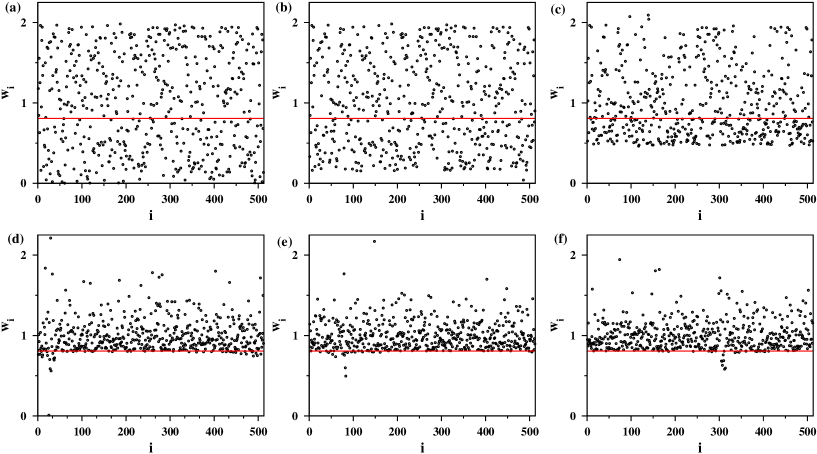
In a linear chain of sites with periodic boundary condition has been considered where the neighbor list of an arbitrary site consists of the two nearest neighboring sites at . Therefore the second agent is selected randomly with equal probability from this list. If is very small then the probability that it will be replaced by an even smaller wealth after trade is also small. However this probability gradually increases as increases. As the sites with the minimal values of wealth are systematically replaced, very soon all nodes with small values are replaced by larger values of resulting a vacancy in the small region. This is explained pictorially in Fig. 1. On an lattice with = 512 we plot the lattice positions along the abscissa and the corresponding wealth along the ordinate. As time increases a vacant region gradually forms for small values of for all sites. If on the average the wealth of none of the agent is below a certain threshold value , it is called the ‘poverty line’. In Fig. 1 the poverty line gradually moves up with time and finally settles at a critical value at the stationary state. This behavior is the same for all system sizes but with different values of . Unlike the model in Ghosh here the critical poverty line is spontaneously determined by the dynamical evolution of the system where no fine tuning is necessary which is the distinctive signature of self-organization and we will see in the following that the model exhibits critical behavior as well.
To find the agent with minimal wealth a brute-force search takes cpu . A much faster algorithm to search for the globally extremal (minimal or maximal) site was proposed by Grassberger Grassberger ; Manna1 which stores the data in a Hierarchical structure. This takes cpu . We have used this method for , and for -clique graphs. For BA graphs we used the brute-force algorithm.
II.1 2.1 Relaxation to Stationary State
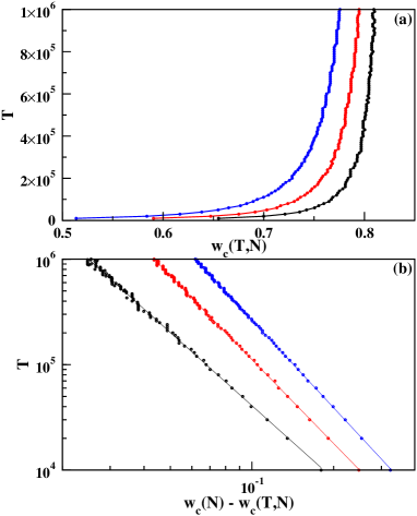
We first estimate the relaxation time required for the system to reach the stationary state. During this relaxation period the wealth distribution gradually changes starting from its initial uniform distribution to its time independent form in the stationary state. The relaxation time has been estimated as a function of deviation of the poverty line from its critical value in two ways.
For a given system size we have simulated our model up to time steps and calculated the wealth distribution at 100 time instants at the interval of steps. These distributions are calculated for a sample size of independent runs. The value of the poverty line at time is determined by the value of where is the maximum. This estimation is done for all values of . In Fig. 2(a) we plot on a scale vs. for , and . We see that in each case the relaxation time diverges as approaches its stationary state value . These data have been replotted in Fig. 2(b) using a scale as vs. where we have used = 0.8242, 0.8375 and 0.8383 to obtain the best straight line plots. The slopes of these straight lines are 2.30, 2.64 and 2.76 respectively which are then extrapolated with to obtain the exponent as with .
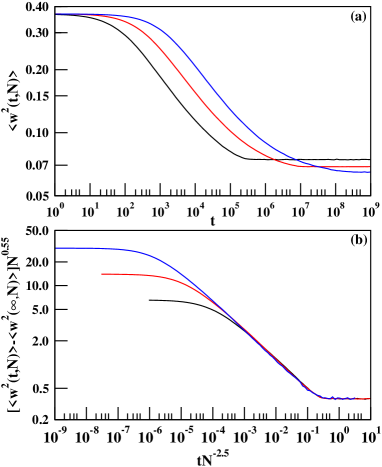
In a second method we calculated with time starting from its initial value when the distribution is uniform. After a long time this quantity saturates to its stationary value . In Fig. 3(a) we show the plots of vs. on a scale. In Fig. 3(b) has been plotted with the scaled value of time using = 0.057, 0.0607 and 0.061 for and respectively. A nice data collapse has been obtained with the following scaling form
| (2) |
where the scaling function varies as for small . A direct measurement of the slope of the scaled plot gives an estimate of which corresponds to . We conclude an average value of .
II.2 2.2 Correlation in the Stationary State
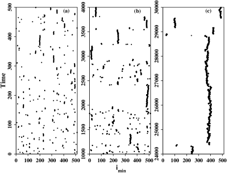
Starting from an uncorrelated wealth distribution the system becomes more and more correlated as time passes. This is reflected in the fact that the probability of occurrence of the minimal sites close to each other in successive time steps gradually increases. At the early uncorrelated stage the position of the minimal site at the next time step is likely to be anywhere in the lattice. However as time increases, the poverty line moves up, consequently increases and the probability that the minimal site at the next time step occurring at the same site or at the neighboring updated site also increases. This is shown in Fig. 4 using a lattice of . For a single run it is observed that the locations of are quite random (Fig. 4(a)). However as time evolves these positions gradually become more correlated (Figs. 4(b) and 4(c)). In general one can consider the successive jumps of positions constituting a Lévy flight random walk Levy . We see below that indeed their flight lengths follow a power law distribution.
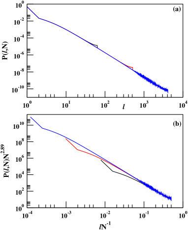
The correlation in the stationary state is quantitatively measured by the probability distribution of the distance of separation between successive minimal sites using periodic boundary condition. This distribution measured in the stationary state has been plotted in Fig. 5(a) for different system sizes and . The value of for = 0 and 1 are approximately 0.4575(1) and 0.4820(1) and then it decreases as a power law with increasing . A direct measurement of slope gives . Fig. 5(b) exhibits the finite-size scaling of the same data when the and axes are scaled as:
| (3) |
where is a universal scaling function with the scaling exponents and . From this scaling analysis we get .
There exists a spatial correlation too in this model. A two point correlation function has been measured in the stationary state. The average correlation between two sites situated at a distance of separation has been defined as:
| (4) |
where is always set equal to unity. We assume a power law decay for the correlation, i.e., for . For a plot of (not shown) vs. on a scale indicates a power law for large values. However considerable variation of slopes exists for system sizes and . The slopes are: -1.17, -1.29. -1.34 respectively which extrapolates to a value of in the limit of . Our estimate for in is 2.2(2).
II.3 2.3 Wealth Distribution in the Stationary State
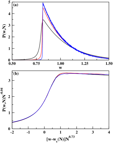
Next we estimated the probability density distribution of wealth in the stationary state of the system of size . The distribution grows very rapidly near for all values of and then decays very fast. In Fig. 6(a) we show the plot of vs. for and . All of them have similar variations but with increasing system size the curves gradually become sharper. Therefore we tried a finite-size scaling analysis in Fig. 6(b) for the growing region and for and . A nice data collapse is observed when axes are scaled and has been plotted with .
The functional form of the decay of the probability distribution has been studied right after the maximal jump at . This part fits very well with the Gaussian form:
| (5) |
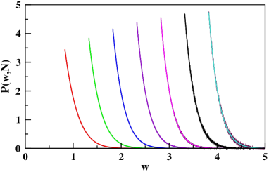
In Fig. 7 we showed vs. on a scale for seven different system sizes: . In each case the fitting curve is indistinguishable from the data. We observe a systematic variation of , and with system size . For example , and .
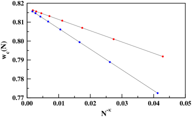
The precise value of is calculated by extrapolating values which are calculated using the following two methods. We have seen in Fig. 6(a) that the probability distribution of becomes increasingly steeper with increasing . For a certain size we defined as the value of for which is half of its maximum value. In a second method the has been calculated in the following way. A pair of successive points on the vs. curve which has the largest slope is found out. A straight line joining these two points is then extrapolated to meet the axis at . The pair of values of and for eight values to are then extrapolated with . A least square fit of straight line has been done for trial values of starting from 0.20 to 1.20 at an interval of 0.001 and the errors have been calculated. The errors are minimal for and . Using these two values of the exponent we extrapolate values with in Fig. 8 to meet the axis at 0.8174 and 0.8176 respectively. We conclude a value for for model as 0.8175(2).
II.4 2.4 Avalanche Size Distribution
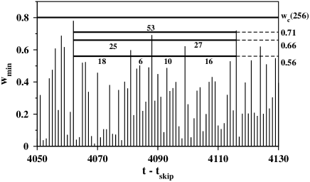
In the stationary state successive values of minimal wealth fluctuates with time. If a certain reference wealth is fixed by hand at then the successive appear below and above line. One defines a -avalanche as the sequence of successive bipartite trades whose values are smaller than . The size of the avalanche measures the duration of the avalanche i.e., at times and the , whereas at every time step from to the . When is set equal to it is called a critical avalanche. This is explained in Fig. 9 where part of the time series for and = 0.8010 is displayed discarding the initial time steps. For an avalanche of size 53 breaks into two avalanches of sizes 25 and and 27 when is reduced to 0.66. On further reduction of to 0.56 these two avalanche break into even smaller avalanches of sizes 18, 6 and 10, 16 respectively. Thus any avalanche can be splitted into a hierarchy of smaller avalanches if value is lowered Paczuski . On the other hand if is raised the average avalanche size increases and becomes infinite at certain value of .
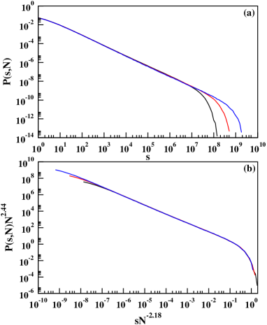
At the critical point the distribution of the avalanche life-times has a power law tail in the limit of : . In the stationary state we used and measured life-times of a large number of avalanches for different system sizes and plot the probability distributions vs. using a scale in Fig. 10(a). Each curve has a straight portion in the intermediate regime of the avalanche sizes and this regime becomes gradually larger on increasing . The direct measurement of slopes in the scaling region gives = 1.086, 1.091 and 1.096 for and respectively. A finite-size scaling is very much suitable with the following scaling form:
| (6) |
where the scaling function in the limit of and approaches zero very fast for . The exponents and fully characterize the scaling of in this case. An immediate way to check the validity of this equation is to attempt a data collapse by plotting vs. with trial values of the scaling exponents. For the values for obtaining the best data collapse are found to be and (Fig. 10(b)). The life-time distribution exponent for is therefore .
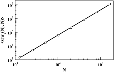
Next we calculated the average value of avalanche life-times right at the critical poverty line. In Fig. 11 we plot this quantity with system size on a scale. The plot fits excellent to a straight line and its slope gives the value of the exponent in: . Assuming the distribution of avalanche sizes holds good up to a cut-off one gets a scaling relation and our estimates of , and satisfy this relation very closely.
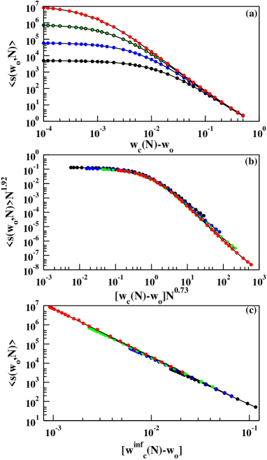
The size of the -avalanches are smaller when and we have studied how the average avalanche size grows as the deviation decreases. Similar to the BS model we assume for . We measured the average size of the -avalanches for different system sizes and plotted them with in Fig. 12(a) with . For all plots on scale the curves are horizontal as deviation is very small. However as the deviation increases the curves become straight with negative slopes -1.98, -2.15, -2.28 and -2.38 for for and respectively. These values when extrapolated with give for . Again a finite-size scaling has been possible as shown in Fig. 12(b):
| (7) |
where is another scaling function. From this data collapse the scaling exponents and with is obtained.
For every system size there is a value of so that when is raised to this value the avalanche size becomes infinite. This implies that if we plot the data in Fig. 12(a) with respect to then we should be able to see the divergence of average avalanche size instead of saturation of the avalanche sizes. We plot this in Fig. 12(c) using = 0.8167, 0.8169, 0.8170, 0.8172 for , , and respectively again on a scale. Each curve is a straight line but with different slopes: -2.31, -2.43, -2.51 and -2.56 respectively. When these slopes are extrapolated with the extrapolated value for is -2.66. Our conclusion for the value of the exponent .
II.5 2.5 Persistence of Wealth in the Stationary State
The time interval between two successive updates of wealth of an agent is known as the persistence time . Different agents have to wait for different amounts of times in general. More specifically agents having small amount of wealth have to wait for very little times. On the other hand potentially rich agents have to wait long enough times. In the stationary state we measure the persistence times for all sites of the lattice and use this data to plot their probability distribution. More precisely we set a clock to each site. Whenever there is a change of wealth at this site the time is noted and the clock time is reset to zero. At the stationary state we collect a large number of persistence time data and use these data to calculate the persistence time distribution.
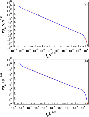
We assume a power law variation of the persistence time distribution as in the limit of . For finite size systems the distributions vs. are plotted on a scale (not shown) and the direct measurement of slopes give the values for finite size systems. These values are extrapolated as to obtain = 1.539 for in . In a similar analysis for a square lattice of size using an extrapolation with respect to we get = 1.25 for .
Persistence exponents are also obtained by the finite-size scaling analysis. In Fig. 13(a) we show the scaling plot of vs. with and . This gives in . Similar scaling analysis in terms of the system size in square lattice has been performed with and which gives = 1.274 (Fig. 13(b)). Averaging values obtained from direct measurement and scaling analysis we conclude in and in .
| Minimal Wealth model | BS model | Manna model | ||||||
|---|---|---|---|---|---|---|---|---|
| BA graph | -clique | |||||||
| 0.8175(2) | 0.6887(2) | 0.6444(2) | 0.6076(2) | 0.66702(8) Grassberger | 0.328855(4) Paczuski | 0.89199(5) Lubeck | 0.68333(3) Lubeck | |
| 1.12(1) | 1.29(1) | 1.50(1) | 1.50(1) | 1.073(3) Grassberger | 1.245(10) Paczuski | 1.112(6) Huynh | 1.273(2) Huynh | |
| 2.65(5) | 1.58(5) | 1.02(5) | 1.00(5) | 2.70(1) Paczuski | 1.70(1) Paczuski | |||
| 2.89(5) | 3.94(5) | - | - | 3.23(2) Paczuski | ||||
| 2.77(7) | ||||||||
| 1.92(2) | 0.95(2) | 0.52(2) | 0.50(2) | 2 | 2 | |||
| 1.541(10) | 1.262(10) | 1.00(1) | 1.00(1) | |||||
III 3. The Maximal Wealth model
Next we studied the Maximal Wealth model where one agent is necessarily the agent with maximal wealth. The other agent being selected randomly with uniform probability from the neighbors of the first agent. Random re-shuffling of wealth takes place in the same way as in the Minimal Wealth model.
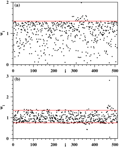
In Fig.14(a) we plot again for the Maximal Wealth model the values of wealth of different agents at a certain instant of time in the stationary state with their positions along an lattice of size . In contrast to the similar plot of the Minimal Wealth model in Fig. 1 here an upper cut-off for the wealth has been visible at .
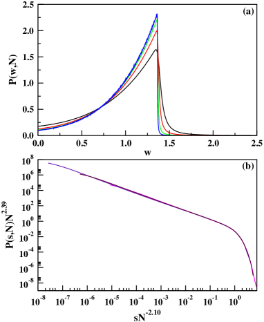
In this case the stationary state wealth distribution takes an opposite shape (Fig. 15(a)). A critical wealth exists here as well. takes a Gaussian form elevated by a constant term for , whereas for it sharply decreases to zero. The parameters of the Gaussian function (Eqn. (4)) are different for different and they vary very systematically with as: , and and the constant .
The critical value of wealth in the asymptotic limit of system sizes has been estimated by the same method as used for the Minimal Wealth model. The and values have been calculated for , , and , extrapolated with and and the asymptotic values are 1.3610 and 1.3608 respectively. We conclude for . A similar analysis gives for square lattice, 1.8895(2) for the BA graph and 1.9998(2) for the -clique.
It may appear that the Minimal Wealth and Maximal Wealth models should be symmetric about the average wealth per agent which we have set at . We have seen above that this indeed not the case since values are 0.8175 and 1.3609 for the Minimal Wealth and Maximal Wealth models respectively. The symmetry between these two models are broken by the presence of a rigid wall at which means that negative value of wealth of an agent is not allowed.
The avalanche size distributions have been studied as well. A finite-size scaling of these distributions has been done and are plotted in Fig. 15(b) using scale as before for and . The scaling exponents are and respectively giving the value of the avalanche size exponent .
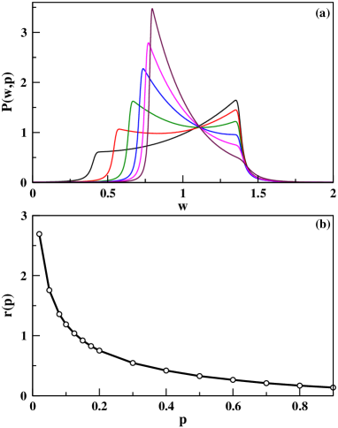
Finally we have studied a mixture of the Minimal Wealth and Maximal Wealth models. At every bipartite trade the first agent with minimal wealth is selected with probability or with maximal wealth with probability . The second agent is selected with uniform probability from the neighbors of the first agent. A snapshot of the individual wealth for at the stationary state for different agents has been shown in Fig. 14(b). Here the wealth values are restriced within a ‘wealth-band’ with sharp cut-offs at a high and a low end. Consequently the shape of the wealth distribution has double peaks for all and we plot the distribution in Fig. 16(a) for . Portion of the distribution between the peaks fits excellent to elevated Gaussian distributions with different parameter values for different values of in the range between 1/2 and 1. On the two sides of this region the distribution decays to zero very fast. The figure shows the plot of vs. for = 0.02, 0.08, 0.2, 0.4, 0.6 and 0.9. In Fig. 16(b) we plot the ratio of the heights of right peak and the left peak with the probability .
IV 4. Conclusion
Social inequality in terms of economic strengths is ubiquitous for the people of all countries. Perhaps this inequality acts as the major driving force behind the advancement of society. Consequently the mechanism that establishes this inequality in a society is an important issue and attracted the attention of researchers over the last century. Here we have studied a modified version of the conservative self-organized extremal model introduced by Pianegonda et. al. which is motivated by the wealth distribution in a society. In this model the entire wealth of the society is strictly conserved. It evolves by a trade dynamics that takes the society from equality (or any other initial wealth distribution) to a stationary state where strong social inequality is present. The dynamics is an infinite sequence of stochastic bipartite tradings where one of the agents has the globally minimal value of wealth, the other one being selected randomly from the neighbors of the first agent. Our numerical study reveals that this model is one of the simplest models of Self-organized Criticality where the stationary state is non-ergodic. This model is very similar to the self-organized critical Bak-Sneppen model for the ecological evolution of interacting species. Using numerical simulation we have estimated a number of critical exponents for this model on an regular lattice, square lattice, the Barabási - Albert scale-free graph and on the -clique graph. We present evidences which suggest that this model does not belong to the universality class of either the Bak-Sneppen model or the Manna model of Self-organized Criticality. This model belongs to a new universality class perhaps because of strict conservation of wealth is maintained in its dynamical rules.
G. Mukherjee thankfully acknowledges the associateship in S. N. Bose National Centre for Basic Sciences, Kolkata under the Extended Visitor and Linkage programme. Comments from B. K. Chakrabarti, A. Chatterjee, D. Dhar, J. R. Iglesias, J. Kertesz, P. K. Mohanty and P. Pradhan are thankfully acknowledged.
manna@bose.res.in
References
- (1) V. Pareto, Cours d’economie Politique (F. Rouge, Lausanne, 1897).
-
(2)
en.wikipedia.org/wiki/Pareto_distribution. - (3) W. Souma, FRACTALS, 9, 463 (2001).
- (4) A. A. Drăgulescu, V. M. Yakovenko, Eur. Phys. J. B 299, 213 (2001).
- (5) J. R. Iglesias, Science and Culture, 76, 437 (2010).
- (6) A. A. Drăgulescu, V. M. Yakovenko, Eur. Phys. J. B 17, 723 (2000).
- (7) V. M. Yakovenko and J. B. Rosser, Rev. Mod. Phys. 81, 1703 (2009).
- (8) J. Angle, Social Forces 65, 293 (1986).
- (9) A. Chakraborti, B. K. Chakrabarti, Eur. Phys. Jour. B, 17 167 (2000).
- (10) K. Bhattacharya, G. Mukherjee and S. S. Manna, in Econophysics of Wealth Distributions, (Springer Verlag, Milan, 2005).
- (11) M. Patriarca, A. Chakraborti, K. Kaski, Phys. Rev. E 70, 016104 (2004).
- (12) A. Chatterjee, B. K. Chakrabarti, S. S. Manna, Physica A 335 155 (2004), A. Chatterjee, B. K. Chakrabarti, S. S. Manna, Physica Scripta T 106 36 (2003).
- (13) P. K. Mohanty, Phys. Rev. E, 74, 011117 (2006).
- (14) U. Basu and P. K. Mohanty, Eur. Phys. J. B 65, 585 (2008).
- (15) A. Chakraborty and S. S. Manna, Phys. Rev. E 81, 016111 (2010).
- (16) A. Chatterjee and B. K. Chakrabarti, Euro. Phys. Journal B 60, 135 (2007).
- (17) S. Pianegonda, J. R. Iglesias, G. Abramson, J. L. Vega, Physica A, 322, 667 (2003).
- (18) J. R. Iglesias, S. Concalves, S. Pianegonda, J. L. Vega and G. Abramson, Physica A, 327, 12 (2003).
- (19) P. Bak and K. Sneppen, Phys. Rev. Lett. 71, 4083 (1993).
- (20) P. Bak, C. Tang and K. Wiesenfeld, Phys. Rev. Lett. 59, 381 (1987).
- (21) P. Bak, How Nature Works: The Science of Self-Organized Criticality, (Copernicus, New York, 1996).
- (22) S.S. Manna, J. Phys. A 24, L363 (1991).
- (23) M. Basu, U. Gayen and P. K. Mohanty, arXiv:1102.1631.
- (24) A. Ghosh, U. Basu, A. Chakraborti and B. K. Chakrabarti, Phys. Rev. E. 83, 061130 (2011).
- (25) S. Lübeck, Int. Jour. Mod. Phys. B 18, 3977 (2004).
- (26) A.-L. Barabási and R. Albert, Science, 286, 509 (1999).
- (27) P. Grassberger, Phys. Lett. A 200, 277 (1995).
- (28) S. S. Manna, Phys. Rev. E., 80, 021132 (2009).
- (29) B. B. Mandelbrot, The Fractal Geometry of Nature, (1982) W.H. Freeman, ISBN 0-7167-186-9.
- (30) M. Paczuski, S. Maslov and P. Bak, Phys. Rev. E 53, 414 (1996).
- (31) S. Lübeck and P. C. Heger, Phys. Rev. lett. 90, 230601 (2003).
- (32) H. N. Huynh, G. Pruessner and L. Y. Chew, J. Stat. Mech. 09024 (2011).